Tracking System for Optical Mobile Communication and the Design Rules
Abstract
Free space optical communication has been applied in many scenarios because of its security, low cost and high rates. In such scenarios, a tracking system is necessary to ensure an acceptable signal power. Free space optical links were considered unable to support optical mobile communication when nodes are randomly moving at a high speed because existing tracking schemes fail to track the nodes accurately and rapidly. In this paper, we propose a novel tracking system exploiting multiple beacon laser sources. At the receiver, each beacon laser’s power is measured to estimate the orientation of the target. Unlike existing schemes which drive servo motors multiple times based on consecutive measurements and feedback, our scheme can directly estimate the next optimal targeting shift for the servo motors based on a single measurement, allowing the tracking system to converge much faster. Closed-form outage probability expression is derived for the optical mobile communication system with ideal tracking, where pointing error and moving statistics are considered. To maintain sufficient average power and reduce the outage probability, the recommended size of a source spot is expressed in closed form as a function of the target’s statistics of random moving, providing insights to the system design.
Index Terms:
Optical mobile communication, outage probability, spot constraints, target mobility, trackingI Introduction
Rapid development of information technology enables us to enjoy more high-quality services while limited frequency bands become increasingly crowded. The exploitation of optical bands can alleviate the shortage of frequency resources and optical wireless communication (OWC) is a promising candidate. OWC refers to the transmission in unguided propagation media through the use of optical carriers, i.e. visible, infrared (IR) and ultraviolet (UV) band [1]. In [1], wide range of applications of OWC were demonstrated from inter-chip connection to inter-satellite links, and outdoor terrestrial OWC links are generally referred to as free space optical (FSO) communication in the literature. The FSO communication mainly suffers from two problems, including atmospheric turbulence and pointing errors. In [2, 3, 4, 5, 6], atmospheric turbulence was divided into weak and strong turbulence cases. The pointing error was modeled by a Rayleigh distributed racial displacement in [6] and the outage probability was finally derived to optimize the design of the FSO links. Reference [7] is a follow-up of [6] which generalized the distribution of the pointing error to Rician distribution, and both bit error rate (BER) and outage probability were derived. However, both [6] and [7] failed to obtain the closed-form expression of the outage probability due to the intractability of turbulence-induced fading.
Unlike traditional radio communication systems, FSO communication systems have high demands on the alignment between the source and the receiver. To achieve accurate alignment, tracking methods are needed to estimate the orientation of the target. In [8], several tracking methods were listed which could be roughly classified into six categories: gimbal-based, mirror-based, gimbal-mirror hybrid, adaptive optics (AO), liquid crystal and RF-FSO hybrid. A gimbal-based method was introduced in [9]. Gimbal is a mechanical device which could perform three-dimensional rotation. In [9], a position sensing diode (PSD) was steered by a gimbal to keep aligned with the laser source in the mobile environment. A mirror-based method was demonstrated in [10] where a mirror actuator with four magnets and four coils was applied, and the electric currents were controlled to change the direction of the mirror in three dimensions. The electric currents were controlled by the light intensity received by quadrant photodiode (QPD) modules. Another mirror-based system was proposed in [11] where two orthogonal mirrors were steered to reflect laser beams by two independent servo motors at the transmitter side. Quad photodiodes were employed at the receiver side to detect the light intensity of the source lasers and an iterative algorithm was applied for tracking based on the detected results of the quad photodiodes. An RF-FSO hybrid tracking system was described in [12] which was applied in a balloon mesh network. In [12], extended kalman filter (EKF) technique was used to keep the links of the balloons aligned. Besides, a non-mechanical tracking system was proposed in [13] which exploited a vertical-cavity surface-emitting laser (VCSEL) array. The lasers in the array were selected according to the direction of the signal received by charge coupled devices (CCDs). This configuration is promising to be applied in multiple-input multiple-output (MIMO) optical systems. All the aforementioned methods need iterative algorithms to approach to the best alignment based on multiple measurements and these algorithms require consecutive feedback from the receiver.
To maintain the stability of FSO systems, the choice of the spot size (or beam width) is an important problem which has been studied in several papers. In [14] and [15], transmitter gain was expressed as a function of the beam width and the BER of an on-off keying (OOK) optical system was calculated. Subsequently, the transmitter gain was optimized according to the calculated BER. In [16], the methods of implementing adaptive beam width were proposed for unmanned aerial vehicles (UAVs). In [17], four optimization models of an FSO channel were formulated. These models were solved in terms of various metrics such as the beam width, electrical signal-to-noise ratio, etc. All the aforementioned papers have applied complicated transmitting models of the laser which may bury some important insights.
In this paper, we consider FSO links shorter than 300 meters, and the receiver has high mobility. Such systems can support optical mobile communications (OMC) [18], and turbulence-induced fading becomes negligible [19]. In the proposed tracking system, there are two types of laser sources which could be divided as the main laser and the beacon lasers. The main laser is responsible for communication while the beacon lasers are applied for tracking the receiver. The aim of the tracking system is to direct the beam of the main laser to the receiver with the help of the beacon lasers. To maintain sufficient signal power for the receiver, closed-form constraints of the main laser’s spot size are developed. The contributions of this work can be summarized as follows:
- •
Closed-form expressions are derived for the average received light power and the outage probability of the OMC link, where pointing error, moving statistics, and beam width are considered.
- •
Exact closed-form spot constraints are derived to ensure sufficient average received power and reduce the outage probability when the target is moving. These constraints could be applied as design rules for OMC systems.
- •
Two types of tracking algorithms are derived to estimate the orientation of the target. Both algorithms exploit maximum likelihood estimation (MLE) [20].
Based on the new analytical results, it is shown that the selection of the main laser’s spot size could dominantly affect the outage probability. After determining several basic parameters of a certain system, the spot size of the main laser could be calculated according to the proposed formula which would provide constructive suggestions for the design of OMC systems.
The paper is organized as follows. System model is given in Section II. Section III derives two constraints of the spot size for the main laser, one is for the average power and the other is for the outage probability. In Section IV, tracking algorithms are designed for the beacon lasers and the simulation results are analyzed in Section V. Section VI shows discussion and Section VII draws concluding remarks.
II System Model
II-A Model of Tracking System
Fig. 1 is a simple demonstration of the tracking system. On the top of the figure, there are one main laser and beacon lasers. The laser at the center of the sources is the main laser which is used for communication between the source and the target. The lasers around the main laser are the beacon lasers which are exploited to track the target. These lasers are fixed on a laser module and the laser module has two steerable axes which could perform three-dimensional rotation to track the target.
The laser sources project their beams onto a two-dimensional reference plane. The beams of the laser sources are parallel with each other and perpendicular to the reference plane. On the reference plane, the target point and the spot centers of the beacon lasers are marked. At the target point, the powers of the beacon beams are measured and fed back to the transmitter as tracking information and the target is able to distinguish the signals of different beacon sources. This can be realized through frequency division, wavelength division, or time division multiplexing.
The aim of the tracking system is to direct the beam center of the main laser to the target point. To this end, accurate estimation of the target point is needed. In other words, the aim of a tracking algorithm is to develop functions and to estimate , i. e.
| (1) |
where is the estimation of ; denotes the measured power of the th beacon laser at the receiver side; is the number of the beacon lasers. Even if the position of the target has been tracked perfectly in a time, the spot center of the main laser is modeled by a random vector because of the unpredictable sway of the laser module. The deviation between the target and the spot center of the main laser is defined as pointing error .
II-B Received Light Signal Intensity and Power
The expression of Gaussian laser’s intensity [21] at distance from the transmitter could be expressed as [6, eq. (7)]
| (2) |
where the vector denotes the radial vector from the spot center of the source laser; denotes the beam width at distance ; is the power coefficient of the source laser and the expression of is
| (3) |
where is the divergence angle of the laser source. The intensity of source light spot at point is modeled as
| (4) |
where is the center of the laser spot. The parameter represents the size of the laser spot. When becomes larger, the spot grows bigger, implying the divergence of power. Assuming that the receiving area of the target is which is relatively small compared with the spot size of the laser, the received signal power at point is
| (5) |
Taking additive noise into consideration, the measured received power is
| (6) |
where denotes the noise, which follows a zero-mean Gaussian distribution, whose probability distribution function (PDF) is
| (7) |
where is the variance of the noise distribution.
II-C Reference Plane

As shown in Fig. 2, the target plane is a two-dimensional surface on which the target moves and the reference plane is a constructed surface which is perpendicular to the beams of the laser sources. On the reference plane, the spots of the lasers are circles which could reduce the complexity of the system.
In Fig. 2, the target locates on the position at the th time interval and has been perfectly tracked, so the beam center of the main laser has been steered to the point at the end of the th time interval. Therefore, the reference plane for the next time interval is constructed which is perpendicular to the main laser and with the point on it. At the next time interval, the target moves to the point on the target plane. To orientate the beam center of the main laser to the new point , is mapped to the point on the reference plane. , and the main laser are collinear. Therefore, we could steer the main laser to by steering it to .
The cross profile in Fig. 2 is demonstrated in Fig. 3. With the help of Fig. 3, we could calculate the light intensities of the points , and as
| (8) |
| (9) |
| (10) |
where is the light intensity defined in (4); is the divergence angle in (3); is the moving distance of the target. According to the similar triangles, is calculated as
| (11) |
thus (10) is expressed as
| (12) |
Taking as a constant, the ratios of the light intensities at the points , and are calculated as
| (13) |
and
| (14) |
where and are also considered as constants. Since the OMC links are mostly over 20 meters, is relatively large compared with and . When ,
| (15) |
which indicates that the light intensities measured on the target plane and the reference plane are exchangeable. This inference is also applicable for the beacon lasers. Therefore, the following parts of this paper is analyzed on the reference plane.
II-D Mobility of Target
In a laser tracking system, the target sends feedback periodically to transmitters, and the transmitters determine the shift of the laser for the next step. In the time interval between two feedback signals, the target position shift on the reference plane follows a two-dimensional Gaussian distribution according to central-limit theorem [22]. This movement pattern is named as Brownian movement [23]. We model the PDF of the target position after a time interval as
| (16) |
where denotes the PDF of the target position on the reference plane at the th time interval; denotes the variance of target distribution; is the point of the target at the th time interval; is the point of the target at the th time interval. The target’s mobility is supposed to be the same on the horizontal and vertical axes, thus and are two independent one-dimensional Gaussian variables which share the same variance . The variance quantifies the uncertainty of the target position in a time interval.11 1 When a variable’s variance and mean are fixed, Gaussian distribution maximizes the entropy of the variable’s distribution [24, Ch. 7.11, pp. 216-217]. Therefore, Gaussian distribution represents the most unpredictable condition of the target distribution.
II-E Pointing Error
The pointing error at the end of the th time interval with ideal tracking is defined as
| (17) |
where is the beam center of the main laser; is the position of the target on the reference plane at the th time interval. The PDF of the pointing error could be modeled by a Rayleigh distribution as
| (18) |
where is a parameter of the Rayleigh distribution. The pointing error will be considered when we constrain the spot size of the main laser.
III Constraints on the Size of Laser Spot
Constraints on the size of the laser spot are designed for the main laser to optimize the power of received signal. In a communication system, if the spot is too large, the laser power may be too dispersed to be distinguished. However, if the spot size is too small, the receiver is unlikely to capture the laser spot due to the pointing error. Therefore, constraints on the spot size should be developed to ensure sufficient average receiving power as well as low outage probability when the pointing error is not negligible. Since the parameter represents the size of the spot, we only need to constrain .
III-A Constraint 1: Maximum Average Received Power
The average intensity at the th time interval received by the target is calculated as
| (19) |
where is defined in (4) and is defined in (16). By solving (19), closed-form expression of is obtained as
| (20) |
where is the pointing error defined in (17). Since follows the Rayleigh distribution with parameter in (18), the expectation over is calculated as
| (21) |
where denotes the expectation. Then the average received power is calculated as
| (22) |
where is the receiving area of the target in (5). To maintain sufficient average received power, is required to be above a threshold as
| (23) |
and the constraint of is solved as
| (24) |
According to (22), if we want to maximize , should be as small as possible. However, when , a slight pointing error will deteriorate the OMC link, thus an additional constraint is necessary.
III-B Constraint 2: Minimum Outage Probability
As shown in the Fig. 4, there are two circles, the right one denotes the target’s distribution and the left one denotes the feasible region with its center at which is also the spot center of the main laser. When the randomly distributed target falls into the feasible region, the received power exceeds the threshold, i.e.
| (25) |
where is the receiving area of the target in (5); is defined in (4); is the threshold. However, if target falls out of the feasible region, the received power is below the threshold, i.e.
| (26) |
Therefore, the feasible region can be defined as
| (27) |
whose boundary is a circle with radius as
| (28) |
where must satisfy
| (29) |
which could be solved as
| (30) |
The outage probability can be expressed as
| (31) |
where the integration region is the feasible region in Fig. 4: ; is defined in (16). The result of (31) could be expressed with the closed-form cumulative distribution function (CDF) of the chi-squared distribution [25]. Therefore, eq. (31) can be simplified to
| (32) |
where is the pointing error, is the Marcum- function, and could be replaced by (28) as
| (33) |
Since follows Rayleigh distribution in (18), the expectation over is calculated as
| (34) |
Equation (34) could be calculated with the [26, eq. (11)] and the result is
| (35) |
By calculating , the minimizing the is obtained as
| (36) |
To reduce the outage probability, is required to be below a threshold as
| (37) |
which could be transformed as
| (38) |
Equation (38) could be solved with Lambert function22 2 Assuming and , the function is the Lambert function. When is below zero, has two values which are denoted as and . . and the result is
| (39) |
where is the Lambert function.
IV Algorithms of Tracking
Tracking algorithms are designed for the beacon lasers to estimate the orientation of the target in terms of the axis of the main laser. In this section the target is considered to be a fixed point in a short time interval and beacon lasers are applied to track the target. According to (1), powers of the beacon beams are measured as
| (40) |
where denotes a vector of measured intensities; is the measured power of the th beacon laser which is defined in (6). Based on , We can estimate the shift between the target and the origin on the reference plane, and based the shift the transmitter can orient the lasers towards the target at the next time interval.
IV-A Algorithm 1: Maximize
According to the maximum likelihood criteria, we can estimate the target coordinates on the reference plane by solving
| (41) |
where is the hypothetical coordinate of the target on the reference plane. The aim of the algorithm is to find the optimal that maximizes the likelihood function . The maximizer is the estimated coordinate of the target projected on the reference plane.
The hypothetical true intensity in the condition of is calculated as
| (42) |
where represents the coordinate of the spot center of the th beacon laser on the reference plane; represents the hypothetical true light intensity of the th beacon laser under the assumption that is the position of target on the reference plane. Then the expression of the noise could be obtained by subtracting from as
| (43) |
where is the receiving area of the target in (5); is the noise related to the th beacon laser. According to (5) and (7), the likelihood function could be calculated as
| (44) |
where is the number of the beacon lasers; denotes the scale of the measured noise which could be estimated by experiments; is the measured power which could be obtained by measurements; is the power coefficient and denotes the spot size which are two adjustable variables; is the coordinate of the spot center of the th beacon laser which is an adjustable and known system parameter.
IV-B Algorithm 2: Maximize
Since the exhaustive method is time-consuming, Algorithm 2 is designed to overcome the drawback of Algorithm 1. According to the maximum likelihood criteria, we can estimate the distance between the target and the spot center of the beacon laser on the reference plane by solving
| (46) |
where is the estimated distance between the spot center of the th beacon laser and the target on the reference plane; is the measured power of the th beacon laser. According to (5) and (7), the likelihood function is calculated as
| (47) |
where is the receiving area of the target in (5); denotes the scale of the measured noise which could be estimated by experiments; is the power coefficient and denotes the spot size which are two adjustable variables. By solving , eq. (46) is solved as
| (48) |
Taking the spot center of the beacon laser as the center and as the radius, circles of different beacon lasers are constructed as
| (49) |
where is the spot center of the th beacon laser; is the target point to be estimated. To get a system of linear equations, the th equation of (49) is subtracted from the th equation of (49) as
| (50) |
which is transformed to
| (51) |
where . According to (51), equations are obtained from (49) as
| (52) |
where . The system of linear equations in (52) could be rewritten as a matrix equation as
| (53) |
where is a matrix, is a matrix as
| (54) |
Since is not necessarily a square matrix, least squares method is exploited to solve the matrix equation in (53) as
| (55) |
where is the estimation of the target point ; is the pseudo-inverse matrix of .
V Simulation Results
V-A Average Received Power
Fig. 5 plots the average received power versus for values of ranging from 40 to 160 with . As shown in the figure, decreases as increases indicating the power divergence of the larger beam width. Besides, when increases, the value of grows, which agrees with (23).
Fig. 6 plots the average received power versus for values of ranging from 1 to 4 with . As grows, the value of declines indicating the larger pointing error or target mobility would deteriorate the OMC link. Besides, when is over 8 meters, the effect of becomes negligible. This implies that a larger spot size counters the fading caused by the target mobility.
V-B Outage probability
Fig. 7 shows the average outage probability as a function of the beam width with and for values of ranging from 40 to 160 . The circles in the figure are the numerical integration results of (34) which agree with (35). As increases from zero meter, declines and then grows, inducing minimums between and . These minimum points could be calculated with (36) which moves to the right as grows. It is also shown that decreases when a larger is exploited. This implies that larger source power could reduce the average outage probability.
Fig. 8 shows the average outage probability as a function of the beam width with and for values of ranging from 1 to 4 . As shown in the figure, the value of increases as grows and when , the minimum value of is less than 0.01. Since would not influence the minimum position of according to (36), the bottom points of the curves share the same value of . This implies that when the parameter is fixed and the requirement of the average outage probability is relatively loose, the best choice of is applicable for various conditions of .
| Parameter | Description | Value |
|---|---|---|
| length of the OMC link in (3) | ||
| product of the power coefficient and the size of the receiving area in (5) | ||
| is defined in (18) and is defined in (16) | ||
| threshold of the average power in (23) | ||
| threshold of the feasible region in (27) | ||
| threshold of the outage probability in (37) |
V-C Example constraints of
In this section, we give an example of spot size constraints exploiting (24) and (39). The parameters of the system are listed in Table I. To keep the average received power more than , the first constraint of is obtained as
| (56) |
To reduce the average outage probability to below , the second constraint of is calculated as
| (57) |
Combining (56) and (57), the final constraint of the main laser’s spot size is obtained as
| (58) |
According to (3), the divergence angle of the main laser is calculated as
| (59) |
thus the range of is
| (60) |
| Parameter | Description | Value |
|---|---|---|
| number of the beacon lasers | ||
| coordinate of the spot center of the th beacon laser on the reference plane, | , , , | |
| coordinate of the spot center of the main laser on the reference plane | ||
| product of the power coefficient and the size of the receiving area | ||
| beam width of the beacon lasers | ||
| standard deviation of the noise | ||
| coordinate of the testing target on the reference plane | ||
| scanning step of the exhaustive method on the reference plane | ||
| searching region of the exhaustive method on the reference plane | a square with as the vertex |


V-D Algorithm 1
In this section, Algorithm 1 designed for the beacon lasers is tested and the basic parameter settings are listed in Table II where four beacon lasers are exploited.
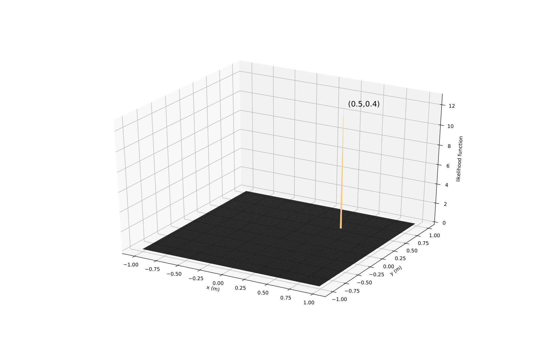
Fig. 9 plots the likelihood in (44) as a function of the and coordinates on the reference plane with the parameters in Table II. As shown in the figure, the likelihood function has one narrow hump which could be searched by the exhaustive method. The hump is exactly on the coordinate of the testing target in Table II indicating that Algorithm 1 is able to track the target.
In Fig. 10, the standard deviation of the noise is change to watt with other parameters unchanged and the likelihood function is plotted. Under the influence of the stronger noise, the hump of the likelihood function becomes larger than that of Fig. 9 and the coordinate of the maximum likelihood value deviates from the target. Similar situation happens when takes a smaller value or becomes bigger.
In Fig. 11, the spot centers of the beacon lasers are changed to , , and with other parameters unchanged and the likelihood function is plotted. The searching region in Table II is modified accordingly. As shown in the figure, a platform appears and the likelihood function could not help us track the target because the spots of the beacon lasers could not cover the target. Similar situation happens when takes a relatively small value.
Therefore, to track the target, here are two notes:
- •
should be big enough compared with to ensure sufficient signal power.
- •
The scales of , and should be close to each other to guarantee that the beams of the beacon lasers could cover the target.
Last but not the least, the exhaustive method takes more than one second to perform a single tracking which is relatively slow for the target tracking.
V-E Algorithm 2
| Parameter | Description | Value |
|---|---|---|
| length of the OMC link | ||
| number of the beacon lasers | ||
| coordinate of the spot center of the th beacon laser on the reference plane, | , , , | |
| coordinate of the spot center of the main laser on the reference plane | ||
| product of the power coefficient and the size of the receiving area | ||
| beam width of the beacon lasers | ||
| standard deviation of the noise |
| Target point | Average tracking error | Average error angle |
|---|---|---|
| 0.0103 | ||
| 0.0119 | ||
| 0.0141 | ||
| 0.0217 | ||
| 0.0430 | ||
| 0.0123 |
Fig. 12 shows the tracking results of Algorithm 2 on the reference plane and the parameters are listed in Table III. Six target points which are listed in Table IV are selected to test the tracking accuracy of Algorithm 2. As shown in Fig. 12, the tracking results are close to the target points and the average tracking errors33 3 The average tracking error is the average deviation between the tracking results and the target point. are also recorded in Table IV. Dividing the average tracking errors by the length of the OMC link in Table III, average error angles are obtained which is at the level of . Besides, the time consumption of Algorithm 2 is much less than that of Algorithm 1 which takes about 0.1 millisecond to perform one tracking.
| Target point | Theoretical error |
|---|---|
| 0.0114 | |
| 0.0118 | |
| 0.0130 | |
| 0.0132 | |
| 0.0232 | |
| 0.0120 |
VI Discussion
VI-A Theoretical Tracking Error
In this section, the theoretical tracking error of the algorithms will be calculated. Equation (5) is rewritten as
| (61) |
where denotes the power of the th beacon laser received by the target; denotes the position of the target on the reference plane; denotes the spot center of the th beacon laser on the reference plane. The total differentials of (61) is
| (62) |
where and . A matrix equation which includes all the beacon lasers is constructed as
| (63) |
where denotes the number of the beacon lasers. From (63), the values of and are calculated as
| (64) |
where is pseudo-inverse matrix of . Therefore, is obtained as
| (65) |
Since denote the discrepancies of the signal, these variables are assumed to be independent and have the same variance . Then the expectations of (65)’s both sides are calculated as
| (66) |
where denotes the trace of ; denotes the variance of . From (66), the theoretical tracking error could be calculated as
| (67) |
The parameters in Table III are exploited to calculate the theoretical tracking error in (67) and the results are listed in Table V. Though the results in Table V are different from the average tracking errors in Table IV44 4 The difference is induced by the least squares method exploited in Algorithm 2., they could provide references for the design of the OMC links.
VII Conclusion
In this paper, several laser sources are exploited to construct a tracking system for the OMC link. These laser sources are divided into a main laser and beacon lasers. The main laser is used for the communication between the transmitter and the target while the beacon lasers are exploited to track the target. To ensure sufficient average power and reduce the outage probability, we constrain the spot size of the main laser considering the mobility of the target and the pointing error of the transmitter. Besides, based on the light powers of the beacon lasers received by the target, two algorithms are designed to track the target. MLE method is adopted to reduce the tracking error. Finally, the closed-form expression of the spot constraints are derived and an OMC tracking system is constructed. These contributions would provide reasonable design rules for optical links.
References
- [1] M. A. Khalighi and M. Uysal, “Survey on free space optical communication: A communication theory perspective,” IEEE communications surveys & tutorials, vol. 16, no. 4, pp. 2231–2258, June 2014.
- [2] L. C. Andrews, R. L. Phillips, C. Y. Hopen, and M. Al-Habash, “Theory of optical scintillation,” JOSA A, vol. 16, no. 6, pp. 1417–1429, June 1999.
- [3] A. Al-Habash, L. C. Andrews, and R. L. Phillips, “Mathematical model for the irradiance probability density function of a laser beam propagating through turbulent media,” Optical Engineering, vol. 40, no. 8, pp. 1554–1563, Feb. 2001.
- [4] X. Zhu and J. M. Kahn, “Free-space optical communication through atmospheric turbulence channels,” IEEE Trans. Commun., vol. 50, no. 8, pp. 1293–1300, Aug. 2002.
- [5] S. M. Flatté, C. Bracher, and G.-Y. Wang, “Probability-density functions of irradiance for waves in atmospheric turbulence calculated by numerical simulation,” JOSA A, vol. 11, no. 7, pp. 2080–2092, July 1994.
- [6] A. A. Farid and S. Hranilovic, “Outage capacity optimization for free-space optical links with pointing errors,” J. Lightw. Technol., vol. 25, no. 7, pp. 1702–1710, July 2007.
- [7] F. Yang, J. Cheng, and T. A. Tsiftsis, “Free-space optical communication with nonzero boresight pointing errors,” IEEE Trans. Commun., vol. 62, no. 2, pp. 713–725, Feb. 2014.
- [8] Y. Kaymak, R. Rojas-Cessa, J. Feng, N. Ansari, M. Zhou, and T. Zhang, “A survey on acquisition, tracking, and pointing mechanisms for mobile free-space optical communications,” IEEE Communications Surveys & Tutorials, vol. 20, no. 2, pp. 1104–1123, Feb. 2018.
- [9] M. K. Al-Akkoumi, H. Refai, and J. J. Sluss Jr, “A tracking system for mobile FSO,” in Free-Space Laser Communication Technologies XX, Feb. 2008, vol. 6877, pp. 68770O.
- [10] H. Urabe, S. Haruyama, T. Shogenji, S. Ishikawa, M. Hiruta, F. Teraoka, T. Arita, H. Matsubara, and S. Nakagawa, “High data rate ground-to-train free-space optical communication system,” Optical Engineering, vol. 51, no. 3, pp. 031204, Mar. 2012.
- [11] S. Muta, T. Tsujimura, and K. Izumi, “Laser beam tracking system for active free-space optical communication,” in Proceedings of the IEEE/SICE International Symposium on System Integration, Dec. 2013, pp. 879–884.
- [12] M. B. Awan and S. Mohan, “Balloon mesh free space optical communication with tracking and link switching,” in 17th International Conference on Transparent Optical Networks (ICTON), July 2015, pp. 1–4.
- [13] M. Toyoshima, N. Miyashita, Y. Takayama, H. Kunimori, and S. Kimura, “System analysis of non-mechanical compact optical transceiver for wireless communications with a VCSEL array,” in 6th International Symposium on Communication Systems, Networks and Digital Signal Processing, July 2008, pp. 187–190.
- [14] S. Arnon, S. Rotman, and N. S. Kopeika, “Beam width and transmitter power adaptive to tracking system performance for free-space optical communication,” Applied optics, vol. 36, no. 24, pp. 6095–6101, Aug. 1997.
- [15] S. Arnon, “Optimization of urban optical wireless communication systems,” IEEE Trans. Wireless Commun., vol. 2, no. 4, pp. 626–629, July 2003.
- [16] K. Heng, N. Liu, Y. He, W. Zhong, and T. Cheng, “Adaptive beam divergence for inter-UAV free space optical communications,” in IEEE PhotonicsGlobal@ Singapore, Dec. 2008, pp. 1–4.
- [17] H. G. Sandalidis, “Optimization models for misalignment fading mitigation in optical wireless links,” IEEE Commun. Lett., vol. 12, no. 5, pp. 395–397, May 2008.
- [18] Z. Zhang, J. Dang, L. Wu, H. Wang, J. Xia, W. Lei, J. Wang, and X. You, “Optical mobile communications: Principles, implementation, and performance analysis,” IEEE Trans. Veh. Technol., vol. 68, no. 1, pp. 471–482, Jan. 2018.
- [19] G. Xu, X. Zhang, J. Wei, and X. Fu, “Influence of atmospheric turbulence on FSO link performance,” Optical Transmission, Switching, and Subsystems, vol. 5281, pp. 816–823, May 2004.
- [20] D. J. MacKay and D. J. Mac Kay, Information theory, inference and learning algorithms. Cambridge: Cambridge university press, 2003.
- [21] B. E. A Saleh and M. C. Teich, Fundamentals of photonics. New York: Wiley, 1991.
- [22] W. Hoeffding, H. Robbins, et al., “The central limit theorem for dependent random variables,” Duke Mathematical Journal, vol. 15, no. 3, pp. 773–780, Jan. 1948.
- [23] J. L. Doob, “The Brownian movement and stochastic equations,” Annals of Mathematics, pp. 351-369, Jan. 1942.
- [24] E. T. Jaynes, Probability theory: The logic of science. Cambridge: Cambridge university press, 2003.
- [25] B. Zhu, J. Cheng, J. Yan, J. Wang, L. Wu and Y. Wang, “A New Asymptotic Analysis Technique for Diversity Receptions Over Correlated Lognormal Fading Channels,” IEEE Trans. Commun., vol. 66, no. 2, pp. 845–861, Feb. 2018.
- [26] A. Nuttall, “Some integrals involving the function (corresp.),” IEEE Trans. Inf. Theory, vol. 21, no. 1, pp. 95–96, Jan. 1975.