The virtual element method for resistive magnetohydrodynamics.

S. Naranjo Alvarez^a, V.A. Bokil^b, V. Gyrya^c, G. Manzini^d

^aDepartment of Mathematics, Oregon State University, Corvallis, OR, 97331,
e-mail: naranjos@math.oregonstate.edu
^bDepartment of Mathematics, Oregon State University, Corvallis, OR, 97331,
e-mail: bokilv@math.oregonstate.edu
^cGroup T-5, Theoretical Division, Los Alamos National Laboratory, Los Alamos, 87545 NM, USA,
e-mail: vitaliy_gyrya@lanl.gov
^dGroup T-5, Theoretical Division, Los Alamos National Laboratory, Los Alamos, 87545 NM, USA,
e-mail: gmanzini@lanl.gov

Abstract

We present a virtual element method (VEM) for the numerical approximation of the electromagnetics subsystem of the resistive magnetohydrodynamics (MHD) model in two spatial dimensions. The major advantages of the virtual element method include great flexibility of polygonal meshes and automatic divergence-free constraint on the magnetic flux field. In this work, we rigorously prove the well-posedness of the method and the solenoidal nature of the discrete magnetic flux field. We also derive stability energy estimates. The design of the method includes three choices for the construction of the nodal mass matrix and criteria to more alternatives. We present a set of numerical experiments that independently validate theoretical results. The numerical experiments include the convergence rate study, energy estimates and verification of the divergence-free condition on the magnetic flux field. All these numerical experiments have been performed on triangular, perturbed quadrilateral and Voronoi meshes. Finally, We demonstrate the development of the VEM method on a numerical model for the Hartmann flow.

Keywords— Maxwell equations, resistive MHD, virtual element method, polytopal mesh, energy stability analysis, Hartmann flow.

1 Introduction

Interest in the behavior of plasmas has skyrocketed in the modern age with applications ranging from fusion-based nuclear power to low power thrusters for contemporary spacecraft. Since the late 1930s, efforts have been devoted to the development of models for plasmas and discretizations that are faithful to the physics and dynamics. An approach that has proven successful and has become standard is to consider plasmas as magnetized fluids, an area called magnetohydrodynamics (MHD). Therefore, the description of these plasmas follow from a blending together of electromagnetic theory and fluid flow. The precise details of how these two theories can be coupled can be found in [34, 46, 44]. Research in MHD is driven by applications that are important to several communities including, astrophysicists that study accretion discs and the dynamics that govern evolution of stars; planetary scientists that are interested in the generation of magnetic fields at the core of planets; plasma physicists whose interest lies in the confinement of plasmas by means of external magnetic fields and engineers who have found that with external magnetic fields they can control the motion of liquid metals leading to a revolution in metallurgical techniques in industry.

The development of numerical methods for MHD is an active area of research, being developed over the last few decades. In [39, 38], two finite element methods are presented that use different techniques in order to preserve the divergence condition on the magnetic field. In [39], the condition is attained automatically, similar to how it is done in this article, whereas in [38] the scheme includes the magnetic vector potential under the temporal gauge, and the magnetic field is obtained as its curl. In [50], the convergence of finite volume methods for MHD is studied and in [45, 32] the classic upwind and Godunov methods are adapted to ideal MHD. In [31], the author presents a finite difference method based on summation by parts (SBP) to mimic the integration by parts formula in the discrete setting, in order to preserve important energy conservation properties and attain an approximate-divergence free scheme. Finally, in [42] the authors develop a MAC scheme for the fluid flow sub-system of the incompressible MHD equations, coupling it to the Yee-scheme for the electromagnetic sub-system.

Although models in MHD come about from a coupling between the equations that govern the fluid flow and Maxwell’s equations for electromagnetism, in this article we will focus on modeling the evolution of the electric and magnetic fields in a plasma for a prescribed fluid flow. Thus, we focus on the Maxwell subsystem of MHD, which combines Faraday’s law, Ampere’s law, Ohm’s law and Gauss’s law for the electromagnetic fields under a prescribed fluid flow.

The main aim of this article is to present a novel numerical discretization of Maxwell’s equations for resistive MHD in a two dimensional setting using the virtual element method (VEM). The VEM was originally proposed in [7] as a variational reformulation of the nodal high-order mimetic finite difference (MFD) method [18, 16, 26], for the numerical treatment of elliptic problems on unstructured polygonal and polyhedral meshes. The word “mimetic” reflects the nature of the method, which mimics the duality and self-adjointness of differential operators as well as identities of vector and tensor calculus. Due to such feature, mimetic methods are often dubbed as compatible methods or compatible discretizations. In particular, satisfying Gauss’s law on the divergence of the magnetic field in the discrete setting requires careful discretization of the Maxwell curl equations, i.e., Faraday’s law and Maxwell-Ampère law. This fact is in contrast to the continuous setting in which the divergence-free nature of the magnetic field is a direct consequence of the Maxwell curl equations when the initial conditions properly satisfy the Gauss’s law.

The violation of Gauss’s law is a serious source of error in the numerical discretization of Maxwell’s equations, causing the appearance of fictitious forces or magnetic monopoles, which are non-physical, thus rendering the numerical simulations unfaithful to the real physics. Over time, mimetic methods were extended from the Support Operator Method (SOM) [48, 49, 40]), which works on regular tensor grids, to the MFD method, which works on fairly general polygonal and polyhedral meshes. The MFD method is, in practice, a family of schemes depending on a set of parameters. These parameters can be optimized to satisfy additional properties such as maximum principles and low dispersion errors. This process goes by the name of mimetic adaptation or M-adaptation and it is outlined in [37]. Previous work in M-adaptation shows that the process can be implemented for problems in wave propagation, see [21], and in the study of cold plasmas, as shown in [22]. Readers interested in historical perspective on the 50-year long development of mimetic and compatible methods are referred to [41]. Development of mimetic and compatible methods are referred to a recent review in [41].

The VEM can also be interpreted as a generalization of the FEM to general polygonal and polyhedral meshes that inherits the great flexibility of the MFD method with respect to the admissible meshes used in the numerical formulation. The major difference when compared to a regular FEM is that in the VEM the shape functions are defined in an implicit manner and never explicitly constructed. The name “virtual element” stems from the fact that such shape functions and the finite element space generated by their linear combinations are, in this sense, “virtual”.

The VEM was originally proposed for solving diffusion problems in [7] as a conforming FEM, and later extended to the nonconforming formulation in [5] and the mixed BDM-like and RT-like formulations in [27] and [10], respectively. Generalizations to convection-reaction-diffusion problems with variable coefficients can be found in [3, 12, 28, 19]. In a series of papers [9, 14, 15, 8], $H(div)$ - and $H(curl)$ -conforming virtual element spaces on general polygonal and polyhedral elements have been proposed to generalize the well known Raviart-Thomas and Nédélec finite elements to unstructured polytopal meshes. These methods, combined with the serendipity strategy that reduces the total number of degrees of freedom, see [11, 13], have successfully been applied to the numerical resolution of the magnetostatic Kikuchi’s model. In these papers, exact virtual de Rham sequences with commuting-diagram interpolation operators are built and the solenoidal nature of the discrete magnetic flux field is ensured. Finally, VEMs have also been designed for hyperbolic problems (see [51, 1]).

In our work, we utilize the low-order spaces proposed in [9], which makes it possible to obtain the combined approximation of the $H^{1}$ -conforming space (0-forms) by a nodal-type virtual element space, the $H(curl)$ -conforming space (1-forms) by an edge-type virtual element space, and the $H(div)$ -conforming space (2-forms) by discontinuous piecewise constant polynomials.

To derive our virtual element approximation, we first reformulate the MHD equations in a variational framework, and then, approximate all $L^{2}$ -type integrals by using suitably defined inner products for nodal-, edge- and cell-type virtual functions. The standard way to build such inner products is through the orthogonal projection of the virtual element functions onto the subspace of linear polynomials. However, as was already noted in [9], the nodal virtual element space that we consider in this work does not provide enough information to construct such projections. Our approach in this paper is to substitute the orthogonal projector with the elliptic projector in [3], since in the low-order case we can always consider these two projection operators as equal by redefining the virtual element space appropriately. This strategy is usually referred to as the “enhanced VEM” by the VEM developers and practitioners.

A major issue occurs here, because changing the definition of the nodal virtual element space requires also changing the definition of the edge and cell virtual element spaces in order to maintain the exact de Rham commuting diagrams. This issue has led to the different virtual element space formulations that were used in the magnetostatics application mentioned above. Instead, in this work we prefer to adopt a different approach, which consists in designing a special reconstruction operator that is computable from the degrees of freedom and stable and bounded as discussed in the following sections. Applying the reconstruction operator makes it possible to recover an approximation of the nodal virtual element functions inside each mesh element and then we integrate directly these reconstructed functions. The choice of the elemental reconstruction operator is not unique. In this work, we considered three different options: the elliptic projection; a Least-Squares interpolation of the nodal values; and the piecewise linear Galerkin interpolation on a triangular sub partition of each element. Our numerical experiments show that these three options are all quite effective and the resulting scheme’s implementations have comparable accuracy.

This article is structured as follows. The rest of this section includes a brief overview of notation and some basic mathematical definitions relevant to the rest of the paper. In Section 2, we present the set of governing equations to be discretized in the continuous setting and introduce the semi-discrete and fully discrete variational formulations in the virtual element framework. Next, in Section 3, we define the virtual element spaces and detail the construction of the inner products that are used for the numerical approximation of the MHD model equations. We also discuss the exactness and commutativity properties of the De-Rham complex and prove that the divergence free condition of the numerical approximation of the magnetic flux field is preserved over time. In Section 4, we prove that the fully discrete variational formulation is well posed. In Section 5, we derive stability energy estimates for the continuous and fully discrete models. In Section 6, we present the results of a series of numerical experiments that provide evidence regarding the convergence rate of the numerical method. Plots demonstrating that the method preserves the divergence free condition of the magnetic flux field are available as well as a numerical study of the energy estimates that are derived theoretically in Section 5. We conclude this section by presenting a simulation of the solution to the Hartmann Flow problem. Then, finally we summarize our findings in section 7.

1.1 Notation, functional spaces and technicalities

We use the standard definition and notation of Sobolev spaces, norms and seminorms, cf. [2]. Let $k$ be a non-negative integer. Consider an open bounded connected subset $\omega$ of $\mathbbm{R}^{2}$ with polygonal boundary $\partial\omega$ . Subset $\omega$ can be the whole computational domain $\Omega$ , or one of the polygonal cells P of the mesh partitioning, $\Omega_{h}$ , covering $\Omega$ .

The Sobolev space $H^{k}(\omega)$ consists of all square integrable functions with all square integrable weak derivatives up to order $k$ that are defined on $\omega$ . As usual, if $k=0$ , we prefer the notation $L^{2}(\omega)$ . Norm and seminorm in $H^{k}(\omega)$ are denoted by $\|\cdot\|_{k,\omega}$ and $|\cdot|_{k,\omega}$ , respectively. We denote the inner product in $L^{2}(\omega)$ by $(\cdot,\cdot)_{\omega}$ , but we omit the subscript when $\omega$ is the whole computational domain $\Omega$ . We denote the norm of an operator $\Pi$ , which is a norm in the dual space, by the general notation $\|\Pi\|$ , regardless of the spaces where range and image of $\Pi$ are defined.

On $\omega$ , we consider the functional spaces:


$\displaystyle L^{2}(\omega)$	$\displaystyle:=\left\{v:\omega\to\mathbbm{R}:\int_{\omega}\|v\|^{2}dV<\infty\right\},$	(1a)
$\displaystyle H(\textbf{rot};\omega)$	$\displaystyle:=\left\{v\in L^{2}(\omega):\textbf{rot}\,v\in\left(L^{2}(\omega)\right)^{2}\right\},$	(1b)
$\displaystyle H(\textrm{div};\omega)$	$\displaystyle:=\left\{\bm{w}\in\left(L^{2}(\omega)\right)^{2}:\textrm{div}\,\bm{w}\in L^{2}(\omega)\right\},$	(1c)
$\displaystyle L^{\infty}(\omega)$	$\displaystyle:=\{\bm{w}:\omega\to\mathbbm{R}:\exists\,C>0\,;\|\bm{w}\|<C\;\mbox{almost everywhere}\},$	(1d)

where $\textbf{rot}\,v=(\partial v/\penalty{\partial y},-\partial v/\penalty{\partial x})^{T}$ , and $\textrm{rot}\,\bm{w}=(\partial w_{x}/\penalty{\partial y}-\partial w_{y}/\penalty{\partial x})$ for the vector field $\bm{w}=(w_{x},w_{y})^{T}$ . If $\omega=\Omega$ denotes the computational domain, we consider the functional spaces:


$\displaystyle V$	$\displaystyle:=\left\{\bm{w}\in H(\textrm{div};\Omega)\,:\,\bm{w}\in\left(L^{2+s}(\Omega)\right)^{2},\ \textrm{for~some~real~}\,s>0\right\},$	(2a)
$\displaystyle H_{0}(\textbf{rot};\Omega)$	$\displaystyle:=\left\{v\in H(\textbf{rot};\Omega)\,:\,v=0\mbox{~on~}\partial\Omega\right\}.$	(2b)

Space $V$ is slightly more regular than $H(\textrm{div};\Omega)$ to ensure that the trace of the normal component ${\bm{v}_{h}\cdot\bm{n}}_{|\textsf{e}}$ on each mesh edge e exists and is continuous across all the internal edges [20].

For an open bounded connected subset $\omega\subset\mathbbm{R}^{d}$ with $d=1$ or $2$ , we denote the linear space of polynomials of degree up to $\ell$ defined on $\omega$ by $\mathbbm{P}_{\ell}(\omega)$ , with the useful conventional notation that $\mathbbm{P}_{-1}(\omega)=\{0\}$ . We denote the space of two-dimensional vector polynomials of degree up to $\ell$ on $\omega$ by $\big[\mathbbm{P}_{\ell}(\omega)\big]^{2}$ . Space $\mathbbm{P}_{\ell}(\omega)$ is the span of the finite set of scaled monomials of degree up to $\ell$ , that are given by

\displaystyle\mathcal{M}_{\ell}(\omega)=\bigg\{\,\left(\frac{\bm{x}-\bm{x}_{\omega}}{h_{\omega}}\right)^{\alpha}\textrm{~with~}|\alpha|\leq\ell\,\bigg\},

where

•

$\bm{x}_{\omega}$ denotes the center of gravity of $\omega$ and $h_{\omega}$ its characteristic length, as, for instance, the edge length or the cell diameter for $d=1,2$ ;
•

$\alpha=(\alpha_{1},\alpha_{2})$ is the two-dimensional multi-index of nonnegative integers $\alpha_{i}$ with degree $|\alpha|=\alpha_{1}+\alpha_{2}\leq\ell$ and such that $\bm{x}^{\alpha}=x_{1}^{\alpha_{1}}x_{2}^{\alpha_{2}}$ for any $\bm{x}\in\mathbbm{R}^{2}$ .

We will also use the set of scaled monomials of degree exactly equal to $\ell$ , denoted by $\mathcal{M}_{\ell}^{*}(\omega)$ and obtained by setting $|\alpha|=\ell$ in the definition above.

Finally, we use the letter $C$ in many inequalities to denote a strictly positive constant whose value can change at any instance. Constant $C$ may depend on the constants of the model equations or the variational problem, like the coercivity and continuity constants, or constants that are uniformly defined for the family of meshes of the approximation while $h\to 0$ , such as the mesh regularity constant, the stability constants of the discrete bilinear forms, etc. However, constant $C$ will never depend on the discretization parameters such as the mesh size $h$ and the timestep $\Delta t$ .

2 The mathematical formulation

Let $\Omega$ be an open, bounded, and polygonal subset of $\mathbbm{R}^{2}$ with boundary $\Gamma=\partial\Omega$ and $T$ a positive real number. For a given fluid flow described by the velocity vector field $\bm{u}=(u_{x},u_{y})^{T}\in\big[L^{\infty}(\Omega)\big]^{2}$ , we consider the Maxwell problem for the electric and magnetic fields, respectively denoted by $E$ and $\bm{B}=(B_{x},B_{y})^{T}$ , that reads as:


$\displaystyle\frac{\partial\bm{B}}{\partial t}$	$\displaystyle=-\textbf{rot}\,E\phantom{\nu\;\textrm{rot}\,\bm{B}\bm{B}^{0}E_{0}(\cdot,t)\quad\textrm{with}\,\,\,\textrm{div}\,\bm{B}^{0}=0}\hskip-56.9055pt\mbox{in~}\Omega\times(0,T],$	(3a)
$\displaystyle E+\bm{u}\times\bm{B}$	$\displaystyle=\nu\;\textrm{rot}\,\bm{B}\phantom{-\textbf{rot}\,E\bm{B}^{0}E_{0}(\cdot,t)\quad\textrm{with}\,\,\,\textrm{div}\,\bm{B}^{0}=0}\hskip-56.9055pt\mbox{in~}\Omega\times(0,T],$	(3b)
$\displaystyle\bm{B}(\cdot,0)$	$\displaystyle=\bm{B}^{0}\quad\textrm{with}\,\,\,\textrm{div}\,\bm{B}^{0}=0\phantom{-\textbf{rot}\,E\nu\;\textrm{rot}\,\bm{B}E_{0}(\cdot,t)}\hskip-56.9055pt\mbox{in~}\Omega,$	(3c)
$\displaystyle E(\cdot,t)$	$\displaystyle=E_{0}(\cdot,t)\phantom{-\textbf{rot}\,E\nu\;\textrm{rot}\,\bm{B}\bm{B}^{0}\quad\textrm{with}\,\,\,\textrm{div}\,\bm{B}^{0}=0}\hskip-56.9055pt\mbox{on~}\partial\Omega\times(0,T],$	(3d)

where $\nu$ is the resistivity of the medium and $\bm{u}\times\bm{B}=u_{x}B_{y}-u_{y}B_{x}$ . We introduce $\sigma=\nu^{-1}$ and assume that it is bounded by two positive constants $\sigma_{*}\leq\sigma(\bm{x})\leq\sigma^{*}$ for almost every $\bm{x}\in\Omega$ . The system of partial differential equations (PDEs) (3) couples Faraday, Ampere and Ohm laws. As discussed in the introduction, an important property of the MHD system (3), which we will address in the virtual element discretization, is the solenoidal nature of the magnetic flux field $\bm{B}$ . By taking the divergence of (3a) we find that the divergence of $\bm{B}$ does not change in time, so $\bm{B}$ is divergence free if the initial field $\bm{B}^{0}$ in (3c) is divergence free.

The variational formulation of problem (3) reads as:

Find $(\bm{B},\widehat{E})\in C^{1}\left([0,T],H(\textrm{div};\Omega)\right)\times C\left([0,T],H_{0}(\textbf{rot};\Omega)\right)$ , such that:


		$\displaystyle\Big(\frac{\partial\bm{B}}{\partial t},\bm{w}\Big)+\Big(\textbf{rot}\,E,\bm{w}\Big)=0\qquad\forall\bm{w}\in H(\textrm{div};\Omega),$		(4a)
		$\displaystyle\Big(\sigma\widehat{E},v\Big)+\Big(\sigma\bm{u}\times\bm{B},v\Big)-\Big(\bm{B},\textbf{rot}\,v\Big)=-\Big(\sigma E_{0},v\Big)\qquad\forall v\in H_{0}(\textbf{rot};\Omega),$		(4b)
		$\displaystyle E=\widehat{E}+E_{0},$		(4c)
		$\displaystyle\bm{B}(\cdot,0)=\bm{B}^{0}\;\;\mbox{with}\;\;\textrm{div}\,\bm{B}^{0}=0.$		(4d)

The boundary conditions on $E$ are set through the known function $E_{0}$ , so we seek for the solution $\widehat{E}$ with zero trace on $\Gamma$ . As is the case of any conforming Galerkin method, we first select subspaces of $H(\textrm{div};\Omega)$ and $H_{0}(\textbf{rot};\Omega)$ defined on the mesh partition $\Omega_{h}$ of the computational domain $\Omega$ . The requirements on the mesh partition $\Omega_{h}$ will be specified in Section 3. We respectively denote them by $\mathcal{E}_{h}$ and $\mathcal{V}_{h}$ , and assume that they are equipped by the inner products $(\cdot,\cdot)_{\mathcal{E}_{h}}$ and $(\cdot,\cdot)_{\mathcal{V}_{h}}$ and suitable interpolation operators, e.g., $\mathcal{I}^{\mathcal{V}_{h}}$ and $\mathcal{I}^{\mathcal{E}_{h}}$ , or projection operator, e.g., $\Pi^{RT}$ . The coefficient $\sigma$ is incorporated in the definition of $\mathcal{V}_{h}$ . We also use the space $\mathcal{V}_{h,0}$ , the subspace of the functions in $\mathcal{V}_{h}$ vanishing at the boundary of $\Omega_{h}$ . The definition and construction of all these mathematical objects are left for the next section. The semi-discrete virtual element discretization of Problem (4) reads as:

Find $(\bm{B}_{h},\widehat{E}_{h})\in C^{1}\left([0,T],\mathcal{E}_{h}\right)\times C\left([0,T],\mathcal{V}_{h,0}\right)$ such that for all $(\bm{w}_{h},v_{h})\in\mathcal{E}_{h}\times\mathcal{V}_{h,0}$ it holds:


		$\displaystyle\Bigg(\frac{\partial\bm{B}_{h}}{\partial t},\bm{w}_{h}\Bigg)_{\mathcal{E}_{h}}+\big(\textbf{rot}\,E_{h},\bm{w}_{h}\big)_{\mathcal{E}_{h}}=0,$		(5a)
		$\displaystyle\big(\widehat{E}_{h},v_{h}\big)_{\mathcal{V}_{h}}+\big(\mathcal{I}^{\mathcal{V}_{h}}\big(\bm{u}\times\Pi^{RT}\bm{B}_{h}\big),v_{h}\big)_{\mathcal{V}_{h}}-\big(\bm{B}_{h},\textbf{rot}\,v_{h}\big)_{\mathcal{E}_{h}}=-\big(\mathcal{I}^{\mathcal{V}_{h}}(E_{0}),v_{h}\big)_{\mathcal{V}_{h}},$		(5b)
		$\displaystyle E_{h}=\widehat{E}_{h}+\mathcal{I}^{\mathcal{V}_{h}}(E_{0}),$		(5c)
		$\displaystyle\bm{B}_{h}(\cdot,0)=\bm{B}^{0}_{h}=\mathcal{I}^{\mathcal{E}_{h}}(\bm{B}^{0})\;\;\mbox{with}\;\;\textrm{div}\,\bm{B}^{0}_{h}=0.$		(5d)

Let $\Delta t$ denote the timestep that splits the time interval $[0,T]$ into $N=T/\penalty{\Delta t}$ subintervals. The virtual element solution pair $\big(\bm{B}_{h}(\cdot,t^{n}),\widehat{E}_{h}(\cdot,t^{n}+\theta\Delta t)\big)$ , with $t^{n}=n\Delta t$ , is approximated by the pair $(\bm{B}_{h}^{n},\widehat{E}_{h}^{n+\theta})$ , which is the solution of the discrete time-dependent problem parameterized by the scalar factor $\theta\in[0,1]$ :

Find $\big\{\bm{B}_{h}^{n}\big\}_{n=0}^{N}\subset\mathcal{E}_{h}$ and $\big\{\widehat{E}_{h}^{n+\theta}\big\}_{n=0}^{N-1}\subset\mathcal{V}_{h,0}$ such that for all $(\bm{w}_{h},v_{h})\in\mathcal{E}_{h}\times\mathcal{V}_{h,0}$ it holds:


		$\displaystyle\Big(\frac{\bm{B}_{h}^{n+1}-\bm{B}_{h}^{n}}{\Delta t},\bm{w}_{h}\Big)_{\mathcal{E}_{h}}+\Big(\textbf{rot}\,E_{h}^{n+\theta},\bm{w}_{h}\Big)_{\mathcal{E}_{h}}=0$		(6a)
		$\displaystyle\big(\widehat{E}_{h}^{n+\theta},v_{h}\big)_{\mathcal{V}_{h}}+\big(\mathcal{I}^{\mathcal{V}_{h}}\big(\bm{u}\times\Pi^{RT}\bm{B}_{h}^{n+\theta}\big),v_{h}\big)_{\mathcal{V}_{h}}-\big(\bm{B}_{h}^{n+\theta},\textbf{rot}\,v_{h}\big)_{\mathcal{E}_{h}}=-\big(\mathcal{I}^{\mathcal{V}_{h}}\big(E_{0}^{n+\theta}\big),v_{h}\big)_{\mathcal{V}_{h}}$		(6b)
		$\displaystyle E_{h}^{n+\theta}=\widehat{E}_{h}^{n+\theta}+\mathcal{I}^{\mathcal{V}_{h}}\big(E_{0}^{n+\theta}\big),$		(6c)
		$\displaystyle\bm{B}_{h}^{n+\theta}=\theta\bm{B}_{h}^{n+1}+(1-\theta)\bm{B}_{h}^{n},$		(6d)
		$\displaystyle\bm{B}_{h}(\cdot,0)=\mathcal{I}^{\mathcal{E}_{h}}\big(\bm{B}^{0}\big).$		(6e)

It is worth noting that $\bm{B}_{h}^{n}$ is defined at the time instants $t^{n}=n\Delta t$ , $n=0,\ldots,N$ , while $\widehat{E}_{h}^{n+\theta}$ is defined on the “staggered” grid at time instants $t^{n+\theta}=(n+\theta)\Delta t$ . According to the $\theta$ parameterization, for $\theta=0$ we recover the explicit or forward Euler scheme, for $\theta=1$ the implicit or backward Euler scheme and for $\theta=1/2$ the (semi) implicit leap-frog scheme.

3 The virtual element method

3.1 Assumptions on mesh regularity

Let $\Omega_{h}=\{\textsf{P}\}$ be a mesh decomposition of $\Omega$ into polygonal element (or cell) P with boundary $\partial\textsf{P}$ , area $|\textsf{P}|$ and diameter $h_{\textsf{P}}$ . As usual, $h=\max_{\textsf{P}\in h}h_{\textsf{P}}$ is the mesh size parameter. We denote the edges of $\partial\textsf{P}$ by e and its length by $|\textsf{e}|=h_{\textsf{e}}$ .

We assume that $h$ belongs to $\mathcal{H}\subset(0,+\infty)$ , which is a countable set of mesh sizes having $0$ as its unique accumulation point. A family of meshes $\{\Omega_{h}\}_{h}$ is said to be regular if there exists a non-negative real number $\rho$ independent of $h$ (and, hence, of $\Omega_{h}$ ), such that

: (M1) (star-shapedness): every polygonal cell P of every mesh $\Omega_{h}$ is star-shaped with respect to every point of a disk of radius $\rho h_{\textsf{P}}$ ;
: (M2) (uniform scaling): every edge $\textsf{e}\in\partial\textsf{P}$ of cell $\textsf{P}\in\Omega_{h}$ satisfies $h_{\textsf{e}}\geq\rho h_{\textsf{P}}$ .

The regularity assumptions (M1)-(M2) allow us to use meshes with cells having quite general geometric shapes. For example, nonconvex cells or cells with hanging nodes on their edges are admissible. Nonetheless, these assumptions have some important implications such as: $(\mathrm{i})$ every polygonal element is simply connected; $(\mathrm{ii})$ the number of edges of each polygonal cell in the mesh family $\{\Omega_{h}\}_{h}$ is uniformly bounded; $(\mathrm{iii})$ a polygonal element cannot have arbitrarily small edges with respect to its diameter $h_{\textsf{P}}\leq h$ for $h\to 0$ and inequality $h_{\textsf{P}}^{2}\leq C(\rho)|\textsf{P}|h_{\textsf{P}}^{2}$ holds, with the obvious dependence of constant $C(\rho)$ on the mesh regularity factor $\rho$ . It is worth mentioning that virtual element methods on polygonal or polyhedral meshes possibly containing “small edges” in 2D or “small faces” in 3D have been considered in [25] for the numerical approximation of the Poisson problem. The work in [25] extends the results in [17] for the original two-dimensional virtual element method to the version of the virtual element method in [3] that can also be applied to problems in three dimensions.

Finally, we note that assumptions $(\mathrm{i})$ - $(\mathrm{iii})$ above also imply that the classical polynomial approximation theory in Sobolev spaces holds [24].

3.2 Nodal virtual element space

On every element $\textsf{P}\in\Omega_{h}$ , we consider the local virtual element space:

\displaystyle\mathcal{V}_{h}(\textsf{P}):=\Big\{\,v_{h}\in H^{1}(\textsf{P})\,:\,{v_{h}}_{|\partial\textsf{P}}\in C^{0}(\partial\textsf{P}),\,{v_{h}}_{|\textsf{e}}\in\mathbbm{P}_{1}(\textsf{e}),\,\forall\textsf{e}\in\partial\textsf{P},\,\Delta v_{h}=0~\textrm{in~}\textsf{P}\,\Big\}.

(7)

Then, we define the global virtual element space:

\displaystyle\mathcal{V}_{h}:=\Big\{\,v_{h}\in H^{1}(\Omega)\,:\,{v_{h}}_{|\textsf{P}}\in\mathcal{V}_{h}(\textsf{P}),\,\,\forall\textsf{P}\in\Omega_{h}\,\Big\};

(8)

The local and global spaces $\mathcal{V}_{h}(\textsf{P})$ and $\mathcal{V}_{h}$ were first proposed in [7]. Space $\mathcal{V}_{h}$ is a subspace of $H^{1}(\Omega)$ , so every virtual element function $v_{h}\in\mathcal{V}_{h}(\textsf{P})$ is continuous over the computational domain $\Omega$ . Every function $v_{h}\in\mathcal{V}_{h}(\textsf{P})$ is uniquely determined by its values at the vertices of P, i.e., by the set $\{v_{h}(\bm{x}_{\textsf{v}})\}_{\textsf{v}\in\partial\textsf{P}}$ . Similarly, a virtual element function in the global space $\mathcal{V}_{h}$ is defined by its values at all the mesh vertices. The unisolvence of such degrees of freedom is proved in [7].

The virtual element schemes (5) and (6) require an approximation of the $L^{2}$ -inner product in $\mathcal{V}_{h}$ . The usual approach to build such an approximation would be through the local orthogonal projection onto the space of linear polynomials, which is a subspace of $\mathcal{V}_{h}(\textsf{P})$ , and by adding a suitable stabilization term. However, the orthogonal projection is not computable from the degrees of freedom of the virtual element functions, namely, the vertex values, unless we change the definition of the elemental space according to the construction proposed in [3]. Here, we prefer not to modify the definition of space $\mathcal{V}_{h}(\textsf{P})$ since otherwise we would lose the property that $\mathcal{V}_{h}$ is in a de Rham complex with space $\mathcal{E}_{h}$ (which will be defined in the next subsection). This topic will be discussed in Section 3.5.

Therefore, for the construction of the approximate $L^{2}$ -inner product in $\mathcal{V}_{h}(\textsf{P})$ , we proceed in two steps. First, for each function $v_{h}\in\mathcal{V}_{h}(\textsf{P})$ , we introduce the linear polynomial approximation $\Pi^{\mathcal{V}_{h}}_{\textsf{P}}v_{h}$ , where operator $\Pi^{\mathcal{V}_{h}}_{\textsf{P}}:H^{1}(\textsf{P})\to\mathbbm{P}_{1}(\textsf{P})$ has these properties:

(V1) the linear polynomial $\Pi^{\mathcal{V}_{h}}_{\textsf{P}}v_{h}$ is computable from the degrees of freedom of $v_{h}$ ;
(V2) operator $\Pi^{\mathcal{V}_{h}}_{\textsf{P}}$ is invariant on linear polynomials, i.e., $\Pi^{\mathcal{V}_{h}}_{\textsf{P}}q=q$ whenever $q$ belongs to $\mathbbm{P}_{1}(\textsf{P})$ ;
(V3) operator $\Pi^{\mathcal{V}_{h}}_{\textsf{P}}$ is uniformly bounded independently of the characteristics of the polygonal element $P$ , i.e. there exists a real constant $C>0$ independent of the number of nodes, edges or diameter of $P$ such that for every $v_{h}\in\mathcal{V}_{h}(\textsf{P})$ one has $\|\Pi^{\mathcal{V}_{h}}_{\textsf{P}}v_{h}\|_{0,\textsf{P}}\leq C\,\|v_{h}\|_{0,\textsf{P}}$ .

Remark 3.1

In Section 3.2.2, the third operator $\Pi^{\mathcal{V}_{h}}_{\textsf{P}}v_{h}$ is defined as the Galerkin piecewise linear interpolant of $v_{h}$ on a triangle subpartition of P. Such subpartition, which we denote by $\textsf{P}_{h}$ , is built by connecting the barycenter of P with its vertices. Therefore, conditions (V1)-(V3) above are set for $\Pi^{\mathcal{V}_{h}}_{\textsf{P}}:H^{1}(\textsf{P})\to\mathbbm{P}_{1}(\textsf{P}_{h})$ , where $\mathbbm{P}_{1}(\textsf{P}_{h})$ is the space of continuous piecewise linear polynomials defined on $\textsf{P}_{h}$ .

In view of mesh regularity assumptions (M1)-(M2) and according to a Bramble-Hilbert argument [23, 35] and property (V2), the approximation error satisfies the upper bound estimate

\displaystyle\|(1-\Pi^{\mathcal{V}_{h}}_{\textsf{P}})v_{h}\|_{0,\textsf{P}}\leq Ch_{\textsf{P}}|v_{h}|_{1,\textsf{P}},

(9)

for every function $v_{h}\in\mathcal{V}_{h}(\textsf{P})\subset H^{1}(\textsf{P})$ and

\displaystyle\|(1-\Pi^{\mathcal{V}_{h}}_{\textsf{P}})v_{h}\|_{0,\textsf{P}}+h_{\textsf{P}}|(1-\Pi^{\mathcal{V}_{h}}_{\textsf{P}})v_{h}|_{1,\textsf{P}}\leq Ch_{\textsf{P}}^{2}|v_{h}|_{2,\textsf{P}}

(10)

whenever $v_{h}\in\mathcal{V}_{h}(\textsf{P})\cap H^{2}(\textsf{P})$ .

Second, we consider the bilinear form on $\mathcal{V}_{h}\times\mathcal{V}_{h}$ given by the formula

\displaystyle\big(v_{h},w_{h}\big)_{\mathcal{V}_{h}}:=\sum_{\textsf{P}\in\Omega_{h}}\big(v_{h},w_{h}\big)_{\mathcal{V}_{h}(\textsf{P})}\qquad\forall v_{h},w_{h}\in\mathcal{V}_{h},

(11)

where each local term $\big(v_{h},w_{h}\big)_{\mathcal{V}_{h}(\textsf{P})}$ is computed by using the elementwise approximations of $v_{h}$ and $w_{h}$ on P according to

\displaystyle\big(v_{h},w_{h}\big)_{\mathcal{V}_{h}(\textsf{P})}:=\big(\sigma\Pi^{\mathcal{V}_{h}}_{\textsf{P}}v_{h},\Pi^{\mathcal{V}_{h}}_{\textsf{P}}w_{h}\big)_{\textsf{P}}+\mathcal{S}^{\mathcal{V}_{h}}_{\textsf{P}}\big((1-\Pi^{\mathcal{V}_{h}}_{\textsf{P}})v_{h},(1-\Pi^{\mathcal{V}_{h}}_{\textsf{P}})w_{h}\big).

(12)

Here, $\mathcal{S}^{\mathcal{V}_{h}}_{\textsf{P}}(\cdot,\cdot)$ is a symmetric and nonnegative bilinear form for which there exist two positive constant $s_{*}$ and $s^{*}$ such that

\displaystyle s_{*}\|v_{h}\|_{0,\textsf{P}}^{2}\leq\mathcal{S}^{\mathcal{V}_{h}}_{\textsf{P}}(v_{h},v_{h})\leq s^{*}\|v_{h}\|_{0,\textsf{P}}^{2}\qquad\forall v_{h}\in\mathcal{V}_{h}(\textsf{P})\cap\textrm{ker}\big(\Pi^{\mathcal{V}_{h}}_{\textsf{P}}{}\big).

(13)

Constants $s_{*}$ and $s^{*}$ are independent of $h$ , but may depend on the regularity parameter $\rho$ and the bounds on $\sigma$ , namely, the two constant factors $\sigma_{*}$ and $\sigma^{*}$ . Effective choices for $\mathcal{S}^{\mathcal{V}_{h}}_{\textsf{P}}(\cdot,\cdot)$ are available from the virtual element literature [43, 33]

3.2.1 Properties of the inner product (12)

In the rest of this section, we investigate the properties of the inner product defined in (12). First, we note that the local bilinear form $(\,\cdot,\cdot\,)_{\mathcal{V}_{h}(\textsf{P})}$ satisfies the consistency condition with respect to the linear polynomials in the sense that $(\,q,p\,)_{\mathcal{V}_{h}(\textsf{P})}=(q,p)_{L^{2}(\textsf{P})}$ for every pair of linear polynomials $q,p$ . This property is more stringent that the usual consistency of the typical virtual element constructions, where the exactness property meaning consistency is true if at least one of the entries is a linear polynomials but not necessarily both simultaneously.

The property that is characterized in the next lemma is the stability of $(\,\cdot,\cdot\,)_{\mathcal{V}_{h}(\textsf{P})}$ with respect to the $L^{2}$ inner product.

Lemma 3.2

There exist two positive constants $\alpha_{*}$ and $\alpha^{*}$ , which are independent of $h$ (and $\Delta t$ ), but may depend on the mesh regularity parameter $\rho$ and the bounds on $\sigma$ , such that

\displaystyle\alpha_{*}\|v_{h}\|_{0,\textsf{P}}^{2}\leq\big(v_{h},v_{h}\big)_{\mathcal{V}_{h}(\textsf{P})}\leq\alpha^{*}\|v_{h}\|_{0,\textsf{P}}^{2}

(14)

for every mesh element P.

Proof. Stability is strictly interconnected with the fact that $(\,\cdot,\cdot\,)_{\mathcal{V}_{h}(\textsf{P})}$ is an inner product in $\mathcal{V}_{h}(\textsf{P})$ . First, we note that $\mathcal{S}^{\mathcal{V}_{h}}_{\textsf{P}}(\cdot,\cdot)$ is a symmetric bilinear form; hence, the bilinear form $(\,\cdot,\cdot\,)_{\mathcal{V}_{h}(\textsf{P})}$ in (12) is also symmetric. The lower bound in (13) implies that $(\,\cdot,\cdot\,)_{\mathcal{V}_{h}(\textsf{P})}$ is bounded from below by the $L^{2}(\textsf{P})$ -norm. Indeed, note that

\displaystyle\big\|v_{h}\big\|_{0,\textsf{P}}^{2}\leq\left(\big\|\Pi^{\mathcal{V}_{h}}_{\textsf{P}}v_{h}\big\|_{0,\textsf{P}}+\big\|(1-\Pi^{\mathcal{V}_{h}}_{\textsf{P}})v_{h}\big\|_{0,\textsf{P}}\right)^{2}\leq 2\Big(\big\|\Pi^{\mathcal{V}_{h}}_{\textsf{P}}v_{h}\big\|_{0,\textsf{P}}^{2}+\big\|(1-\Pi^{\mathcal{V}_{h}}_{\textsf{P}})v_{h}\big\|_{0,\textsf{P}}^{2}\Big).

Then, a straightforward calculation yields the chain of inequalities:

	$\displaystyle\big(v_{h},v_{h}\big)_{\mathcal{V}_{h}(\textsf{P})}$	$\displaystyle\geq\sigma_{}\big\\|\Pi^{\mathcal{V}_{h}}_{\textsf{P}}v_{h}\big\\|_{0,\textsf{P}}^{2}+s_{}\big\\|(1-\Pi^{\mathcal{V}_{h}}_{\textsf{P}})v_{h}\big\\|_{0,\textsf{P}}^{2}$
		$\displaystyle\geq\min(\sigma_{},s_{})\Big(\big\\|\Pi^{\mathcal{V}_{h}}_{\textsf{P}}v_{h}\big\\|_{0,\textsf{P}}^{2}+\big\\|(1-\Pi^{\mathcal{V}_{h}}_{\textsf{P}})v_{h}\big\\|_{0,\textsf{P}}^{2}\Big)\geq\alpha_{*}\big\\|v_{h}\big\\|_{0,\textsf{P}}^{2},$

where we set $\alpha_{*}=\min(\sigma_{*},s_{*})/\penalty{2}$ .

The inequality from above is proved in a similar way:

	$\displaystyle\big(v_{h},v_{h}\big)_{\mathcal{V}_{h}(\textsf{P})}$	$\displaystyle=\big(\sigma\Pi^{\mathcal{V}_{h}}_{\textsf{P}}v_{h},\Pi^{\mathcal{V}_{h}}_{\textsf{P}}v_{h}\big)+\mathcal{S}^{\mathcal{V}_{h}}_{\textsf{P}}((1-\Pi^{\mathcal{V}_{h}}_{\textsf{P}})v_{h},(1-\Pi^{\mathcal{V}_{h}}_{\textsf{P}})v_{h})$
		$\displaystyle\leq(\sigma^{}+s^{})\Big(\\|\Pi^{\mathcal{V}_{h}}_{\textsf{P}}v_{h}\\|_{0,\textsf{P}}^{2}+\\|(1-\Pi^{\mathcal{V}_{h}}_{\textsf{P}})v_{h}\\|_{0,\textsf{P}}^{2}\Big)\leq\alpha^{*}\\|v_{h}\\|_{0,\textsf{P}}^{2},$

where we set $\alpha^{*}=(\sigma^{*}+s^{*})\big(1+\|\Pi^{\mathcal{V}_{h}}_{\textsf{P}}\|\big)^{2}$ in the final step.

Remark 3.3

A suitable choice of $\mathcal{S}^{\mathcal{V}_{h}}_{\textsf{P}}$ and its scaling factor may allow us to have $s^{*}=\sigma^{*}$ . Also, we can define $\Pi^{\mathcal{V}_{h}}_{\textsf{P}}$ so that $\|\Pi^{\mathcal{V}_{h}}_{\textsf{P}}\|\leq 1$ . This implies that $\alpha^{*}\leq 2\sigma^{*}$ and we can use this bound in the inequalities of the next sections to have an explicit dependence on $\sigma^{*}$ .

The two properties of symmetry and non-negativity imply that $(\,\cdot,\cdot\,)_{\mathcal{V}_{h}(\textsf{P})}$ is an inner product in $\mathcal{V}_{h}(\textsf{P})$ for any element $\textsf{P}\in\Omega_{h}$ , so that the quantity

\displaystyle|\hskip-0.56905pt|\hskip-0.56905pt|v_{h}|\hskip-0.56905pt|\hskip-0.56905pt|_{{}_{\mathcal{V}_{h}(\textsf{P})}}^{2}:=\big(v_{h},v_{h}\big)_{\mathcal{V}_{h}(\textsf{P})}

is the induced local norm and the Cauchy-Schwarz inequality must hold

\displaystyle\big(v_{h},w_{h}\big)_{\mathcal{V}_{h}(\textsf{P})}\leq|\hskip-0.56905pt|\hskip-0.56905pt|v_{h}|\hskip-0.56905pt|\hskip-0.56905pt|_{{}_{\mathcal{V}_{h}(\textsf{P})}}|\hskip-0.56905pt|\hskip-0.56905pt|w_{h}|\hskip-0.56905pt|\hskip-0.56905pt|_{{}_{\mathcal{V}_{h}(\textsf{P})}}\qquad\forall v_{h},w_{h}\in\mathcal{V}_{h}(\textsf{P}).

(15)

By summing over all the mesh elements, we find that the symmetric bilinear form defined in (11) is bounded from below by the $L^{2}(\Omega)$ -norm. Therefore, equation (11) defines an inner product on the global virtual element space $\mathcal{V}_{h}$ , with induced norm given by

\displaystyle|\hskip-0.56905pt|\hskip-0.56905pt|v_{h}|\hskip-0.56905pt|\hskip-0.56905pt|_{{}_{\mathcal{V}_{h}}}^{2}:=\sum_{\textsf{P}\in\Omega_{h}}\big(v_{h},v_{h}\big)_{\mathcal{V}_{h}(\textsf{P})}.

We readily see that such inner product is continuous with respect to its induced norm

\displaystyle\big(v_{h},w_{h}\big)_{\mathcal{V}_{h}}\leq|\hskip-0.56905pt|\hskip-0.56905pt|v_{h}|\hskip-0.56905pt|\hskip-0.56905pt|_{{}_{\mathcal{V}_{h}}}|\hskip-0.56905pt|\hskip-0.56905pt|w_{h}|\hskip-0.56905pt|\hskip-0.56905pt|_{{}_{\mathcal{V}_{h}}}\qquad\forall v_{h},w_{h}\in\mathcal{V}_{h},

(16)

and such norm is bounded from below by the $L^{2}$ norm

\displaystyle|\hskip-0.56905pt|\hskip-0.56905pt|v_{h}|\hskip-0.56905pt|\hskip-0.56905pt|_{{}_{\mathcal{V}_{h}}}^{2}=\big(v_{h},v_{h}\big)_{\mathcal{V}_{h}}\geq\alpha_{*}\big\|v_{h}\big\|_{0,\Omega}^{2}.

(17)

Likewise, in view of Lemma 3.2, the global inner product is also continuous with respect to the $L^{2}(\textsf{P})$ -inner product. In fact, on starting from (16) and using the upper bound in (14), we find that

\displaystyle\big(v_{h},w_{h}\big)_{\mathcal{V}_{h}(\textsf{P})}\leq|\hskip-0.56905pt|\hskip-0.56905pt|v_{h}|\hskip-0.56905pt|\hskip-0.56905pt|_{{}_{\mathcal{V}_{h}(\textsf{P})}}|\hskip-0.56905pt|\hskip-0.56905pt|w_{h}|\hskip-0.56905pt|\hskip-0.56905pt|_{{}_{\mathcal{V}_{h}(\textsf{P})}}\leq\alpha^{*}\|v_{h}\|_{0,\textsf{P}}\,\|w_{h}\|_{0,\textsf{P}},

(18)

where we recall that $\alpha^{*}=(\sigma^{*}+s^{*})\big(1+\|\Pi^{\mathcal{V}_{h}}\|\big)^{2}$ . By summing all the local terms and noting that $h\geq h_{\textsf{P}}$ for every P yields:

\displaystyle\big(v_{h},w_{h}\big)_{\mathcal{V}_{h}}\leq\,\alpha^{*}\big\|v_{h}\big\|_{0,\Omega}\,\|w_{h}\|_{0,\Omega}.

(19)

Therefore, the local inner product is continuous with respect to the $L^{2}(\textsf{P})$ -norm for every $\textsf{P}\in\Omega_{h}$ and the global inner product in $\mathcal{V}_{h}$ is continuous with respect to the $L^{2}(\Omega)$ -norm.

3.2.2 Construction of operator $\Pi^{\mathcal{V}_{h}}_{\textsf{P}}$

We discuss three different choices for the approximation operator $\Pi^{\mathcal{V}_{h}}_{\textsf{P}}$ .

(I).Elliptic projection operator(E). The most obvious example of such a computable approximation operator is the elliptic projection of a virtual element function $v_{h}\in\mathcal{V}_{h}(\textsf{P})$ , which is the linear polynomial $\Pi^{\nabla}_{\textsf{P}}v_{h}$ solving the variational problem:

	$\displaystyle\int_{\textsf{P}}\nabla\Pi^{\nabla}_{\textsf{P}}v_{h}\cdot\nabla q_{h}dV$	$\displaystyle=\int_{\textsf{P}}\nabla v_{h}\cdot\nabla q_{h}dV\qquad\forall q_{h}\in\mathbbm{P}_{1}(\textsf{P}),$		(20)
	$\displaystyle\frac{1}{N_{\textsf{v}}}\sum_{v\in P}\Pi^{\nabla}_{\textsf{P}}v_{h}$	$\displaystyle=\frac{1}{N_{\textsf{v}}}\sum_{v\in P}v_{h}.$		(21)

The elliptic projection $\Pi^{\nabla}_{\textsf{P}}v_{h}$ clearly provides a linear polynomial approximation of $v_{h}$ , which is computable from the degrees of freedom, (V1), and invariant on linear polynomials, (V2), cf. Ref. [3]. Property (V3) is proved in the appendix, see Section A.

(II). Least Squares reconstruction operator(LS). An alternative to the elliptic projection operator is provided by the linear interpolant

\displaystyle\Pi^{LS}_{\textsf{P}}v_{h}(x,y)=a+b\frac{x-x_{\textsf{P}}}{h_{\textsf{P}}}+c\frac{y-y_{\textsf{P}}}{h_{\textsf{P}}},

(22)

where the three real coefficients $a,b,c$ are determined by imposing that

\displaystyle\Pi^{LS}_{\textsf{P}}v_{h}(x_{\textsf{v}},y_{\textsf{v}})=a+b\frac{x_{\textsf{v}}-x_{\textsf{P}}}{h_{\textsf{P}}}+c\frac{y_{\textsf{v}}-y_{\textsf{P}}}{h_{\textsf{P}}}=v_{h}(x_{\textsf{v}},y_{\textsf{v}})\qquad\forall\textsf{v}\in\partial\textsf{P},

(23)

where $\bm{x}_{\textsf{v}}=(x_{\textsf{v}},y_{\textsf{v}})^{T}$ is the coordinate position vector of vertex v. We solve the resulting system using the Least Squares method. Indeed, this system has $N^{\mathcal{V}}_{\textsf{P}}$ equations where $N^{\mathcal{V}}_{\textsf{P}}$ is the number of vertices of the polygonal element and only three unknowns, and is overdetermined unless P is a triangular cell. The linear polynomial $\Pi^{LS}_{\textsf{P}}v_{h}$ only depends on the vertex values of $v_{h}$ and is clearly computable (property (V1)) and is invariant on the linear polynomials (property (V2)). Property (V3) is proved in the appendix, see Section B.

(III). Galerkin interpolation operator(GI). The third alternative that we consider in this paper is given by a finite element-like piecewise linear interpolant on the polygonal cell P. Assumptions (M1)-(M2) imply the existence of an internal point $\textsf{v}^{*}$ with respect to which P must be star-shaped (e.g., the center of the disk in (M1)). We assume that this point is described by the coordinate vector

\displaystyle\bm{x}^{*}_{\textsf{P}}=\sum_{\textsf{v}\in\partial\textsf{P}}\omega_{\textsf{P},\textsf{v}}\bm{x}_{\textsf{v}},\qquad\textrm{with}\quad 0<\omega_{\textsf{P},\textsf{v}}<1\quad\textrm{and}\quad\sum_{\textsf{v}\in\partial\textsf{P}}\omega_{\textsf{P},\textsf{v}}=1,

where the weights $\omega_{\textsf{P},\textsf{v}}$ are known. For example, if P is convex, we can choose the arithmetic average of the vertex positions, so $\omega_{\textsf{P},\textsf{v}}=1/\penalty{N^{\mathcal{V}}_{\textsf{P}}}$ , or the baricenter of P. Then, we approximate $v_{h}(\bm{x}^{*}_{\textsf{P}})$ by the average of the vertex values using the same weights $\omega_{\textsf{P},\textsf{v}}$ :

\displaystyle v_{h}(\bm{x}^{*}_{\textsf{P}})\approx v_{\textsf{P}}^{*}=\sum_{\textsf{v}\in\partial\textsf{P}}\omega_{\textsf{P}\textsf{v}}v_{h}(\bm{x}_{\textsf{v}}).

(24)

We note that $v_{h}(\bm{x}^{*}_{\textsf{P}})=v_{\textsf{P}}^{*}$ if $v_{h}$ is a linear polynomial, which is crucial to ensure that property (V2) is satisfied. We connect the internal point $\textsf{v}^{*}$ to all the vertices $\textsf{v}\in\Omega_{h}$ , thus splitting P in $N^{\mathcal{V}}_{\textsf{P}}$ subtriangles T that form a patch around $\textsf{v}^{*}$ . The patch nodes are the vertices of the polygonal boundary of P and vertex $\textsf{v}^{*}$ . Let $\phi_{\textsf{v}}(\bm{x}_{\textsf{v}})$ be the continuous piecewise linear function defined on the patch that is one at a given patch node (including vertex $\textsf{v}^{*}$ ) and zero at the other nodes. Finally, we define the operator $\Pi^{\mathcal{V}_{h}}_{\textsf{P}}:H^{1}(\textsf{P})\to\mathbbm{P}_{1}(\textsf{P}_{h})$ (see Remark 3.1) by

\displaystyle\Pi^{pw}_{\textsf{P}}v_{h}(\bm{x})=\sum_{\textsf{v}\in\partial\textsf{P}}v_{h}(\bm{x}_{\textsf{v}})\phi_{\textsf{v}}(\bm{x})+v_{\textsf{P}}^{*}\phi_{\textsf{v}^{*}}(\bm{x}),

(25)

which is the continuous piecewise linear interpolant of $v_{h}$ on the set of values $\{(\bm{x}_{\textsf{v}},v_{h}(\bm{x}_{\textsf{v}}))\}_{\textsf{v}\in\Omega_{h}}\cup\{(\bm{x}_{\textsf{v}^{*}},v_{\textsf{P}}^{*})\}$ . From this construction it is obvious that $\Pi^{pw}_{\textsf{P}}v_{h}$ is computable from the vertex values of $v_{h}$ (property (V1)); $\Pi^{pw}_{\textsf{P}}q=q$ if $q$ is a linear polynomial (property (V2)); $\Pi^{pw}_{\textsf{P}}v_{h}$ is bounded (property (V3)) since $0\leq\phi_{\textsf{v}}(\bm{x})\leq 1$ for all the patch functions $\phi_{\textsf{v}}$ at every patch node $\bm{x}_{\textsf{v}}$ and $\phi_{\textsf{v}^{*}}$ at $\bm{x}^{*}$ .

3.3 Edge virtual element space

On every element $\textsf{P}\in\Omega_{h}$ , we consider the following finite-dimensional space:

\displaystyle\mathcal{E}_{h}(\textsf{P}):=\big\{\bm{v}_{h}\in H(\textrm{div};\textsf{P})\cap H(\textrm{rot};\textsf{P}):

\displaystyle{\bm{v}_{h}\cdot\bm{n}}_{|\textsf{e}}\in\mathbbm{P}_{0}(\textsf{e})\,\forall\textsf{e}\in\partial\textsf{P},\,\textrm{div}\,\bm{v}_{h}\in\mathbbm{P}_{0}(\textsf{P})~\textrm{and}~\textrm{rot}\,\bm{v}_{h}=0~\textrm{in}~\textsf{P}\big\}.

(26)

The local virtual element space $\mathcal{E}_{h}(\textsf{P})$ was introduced in the VEM literature in Ref. [10]. It is worth noting that on a triangular cell, space $\mathcal{E}_{h}(\textsf{P})$ coincides with the space of vector-valued polynomials $\textrm{RT}_{0}(\textsf{P})=(\mathbbm{P}_{0}(\textsf{P}))^{2}+\mathbbm{P}_{0}(\textsf{P})\bm{x}$ , i.e., those vector-valued fields that are of the form $\bm{w}(\bm{x})=\bm{a}+b\bm{x}$ for some vector and scalar coefficients $\bm{a}\in\mathbbm{R}^{2}$ and $b\in\mathbbm{R}$ , respectively; see [20]. In the case of a general polygonal cell, $\big(\mathbbm{P}_{0}(\textsf{P})\big)^{2}$ and $\textrm{RT}_{0}(\textsf{P})$ are clearly subspaces of $\mathcal{E}_{h}(\textsf{P})$ . In view of this elemental definition, we have the corresponding global virtual element space:

\displaystyle\mathcal{E}_{h}:=\Big\{\,\bm{v}_{h}\in V\,:\,{\bm{v}_{h}}_{|\textsf{P}}\in\mathcal{E}_{h}(\textsf{P}),\,\forall\textsf{P}\in\Omega_{h}\,\Big\}.

(27)

By definition, space $\mathcal{E}_{h}$ is a subspace of $V$ . Each virtual element function $\bm{v}_{h}\in\mathcal{E}_{h}(\textsf{P})$ is uniquely defined by the values of its normal components at the edges of P, $\{{\bm{v}_{h}\cdot\bm{n}}_{|\textsf{e}}\}_{\textsf{e}\in\partial\textsf{P}}$ . Similarly, a virtual function in the global space $\mathcal{E}_{h}$ is defined by the values of its normal components at the mesh edges. The unisolvence of this set of degrees of freedom for $\mathcal{E}_{h}$ is proved in [10].

In $\mathcal{E}_{h}$ we can compute the two different orthogonal projection operators denoted by $\Pi^{\mathcal{E}_{h}}_{\textsf{P}}$ and $\Pi^{RT}_{\textsf{P}}$ , which respectively project from $H(\textrm{div};\textsf{P})$ onto $\big[\mathbbm{P}_{0}(\textsf{P})\big]^{2}$ and $\textrm{RT}_{0}(\textsf{P})$ . The orthogonal projection $\Pi^{\mathcal{E}_{h}}_{\textsf{P}}\bm{v}$ is the constant vector field solving the variational problem

\displaystyle\int_{\textsf{P}}\Pi^{\mathcal{E}_{h}}_{\textsf{P}}\bm{v}_{h}\cdot\bm{q}_{h}dV=\int_{\textsf{P}}\bm{v}_{h}\cdot\bm{q}_{h}dV,\qquad\forall\bm{q}_{h}\in\big[\mathbbm{P}_{0}(\textsf{P})\big]^{2}.

This operator is computable from the degrees of freedom, cf. [10].

Also, $\Pi^{RT}_{\textsf{P}}\bm{v}_{h}$ is the (unique) solution of the following variational problem:

\displaystyle\int_{\textsf{P}}\Pi^{RT}_{\textsf{P}}\bm{v}_{h}\cdot\bm{w}_{h}dV=\int_{\textsf{P}}\bm{v}_{h}\cdot\bm{w}_{h}dV,\qquad\forall\bm{w}_{h}\in\textrm{RT}_{0}(\textsf{P}).

We show here that $\Pi^{RT}_{\textsf{P}}\bm{v}_{h}$ is computable from the degrees of freedom $\bm{v}_{h}\in\mathcal{E}_{h}$ . Since $\bm{w}_{h}(\bm{x})=\bm{a}+b\bm{x}$ , we write it as the gradient of a second-degree polynomial, i.e., $\bm{w}_{h}=\nabla q$ where $q(\bm{x})=\bm{a}\cdot\bm{x}+(b/2)\bm{x}^{T}\bm{x}$ . Then, we substitute this expression for $\bm{w}_{h}$ in the right-hand side, integrate by parts and obtain:

\displaystyle\int_{\textsf{P}}\bm{v}_{h}\cdot\bm{w}_{h}dV=\int_{\textsf{P}}\bm{v}_{h}\cdot\nabla q\ dV=-\int_{\textsf{P}}(\textrm{div}\,\bm{v}_{h})q\ dV+\sum_{\textsf{e}\in\partial\textsf{P}}\int_{\textsf{e}}\bm{n}\cdot\bm{v}_{h}\,q\ dS.

All the integrals on the right-hand side are computable. In fact, the values ${\bm{n}\cdot\bm{v}_{h}}_{|\textsf{e}}$ for all edges $\textsf{e}\in\partial\textsf{P}$ are known as they are the degrees of freedom of $\bm{v}_{h}$ . Moreover, the divergence of $\bm{v}_{h}$ is also known as it is constant over P and a straightforward application of the Gauss Divergence theorem yields:

\displaystyle\textrm{div}\,\bm{v}_{h}=\frac{1}{|\textsf{P}|}\sum_{\textsf{e}\in\partial\textsf{P}}|\textsf{e}|{\bm{n}\cdot\bm{v}_{h}}_{|\textsf{e}}.

A similar argument can be used to prove that $\Pi^{\mathcal{E}_{h}}_{\textsf{P}}\bm{v}_{h}$ is computable from the degrees of freedom of $\bm{v}_{h}$ (take $q_{h}=\bm{a}\cdot\bm{x}$ ), see Ref. [10].

We use the orthogonal projector onto the constant vector fields to define the inner product in $\mathcal{E}_{h}$ . As usual in the VEM, we split it into the sum of local contributions:

\displaystyle\big(\bm{v}_{h},\bm{w}_{h}\big)_{\mathcal{E}_{h}}=\sum_{\textsf{P}\in\Omega_{h}}\big(\bm{v}_{h},\bm{w}_{h}\big)_{\mathcal{E}_{h}(\textsf{P})},

(28)

where each local term is the inner product in $\mathcal{E}_{h}(\textsf{P})$ and takes the form

\displaystyle\big(\bm{v}_{h},\bm{w}_{h}\big)_{\mathcal{E}_{h}(\textsf{P})}=(\Pi^{\mathcal{E}_{h}}_{\textsf{P}}\bm{v}_{h},\Pi^{\mathcal{E}_{h}}_{\textsf{P}}\bm{w}_{h})_{\textsf{P}}+\mathcal{S}^{\mathcal{E}_{h}}_{\textsf{P}}\big((1-\Pi^{\mathcal{E}_{h}}_{\textsf{P}})\bm{v}_{h},(1-\Pi^{\mathcal{E}_{h}}_{\textsf{P}})\bm{w}_{h}\big)

(29)

and again we assume that $\mathcal{S}^{\mathcal{E}_{h}}_{\textsf{P}}(\cdot,\cdot)$ is a symmetric and nonnegative bilinear form for which there exist two positive constant $\bar{s}_{*}$ and $\bar{s}^{*}$ such that

\displaystyle\bar{s}_{*}\|\bm{v}_{h}\|_{0,\textsf{P}}^{2}\leq\mathcal{S}^{\mathcal{E}_{h}}_{\textsf{P}}(v_{h},v_{h})\leq\bar{s}^{*}\|\bm{v}_{h}\|_{0,\textsf{P}}^{2}\qquad\forall v_{h}\in\mathcal{E}_{h}(\textsf{P})\cap\textrm{ker}\big(\Pi^{\mathcal{E}_{h}}_{\textsf{P}}{}\big).

Since $\Pi^{\mathcal{E}_{h}}_{\textsf{P}}$ is the orthogonal projection onto the constant vector-valued fields defined on P, it is now easy to prove that this inner product is consistent and stable in the usual VEM sense; namely,

•

consistency:

\displaystyle\big(\bm{v}_{h},\bm{q}_{h}\big)_{\mathcal{E}_{h}(\textsf{P})}=\int_{\textsf{P}}\bm{v}_{h}\cdot\bm{q}_{h}dV\qquad\bm{q}_{h}\in\big(\mathbbm{P}_{0}(\textsf{P})\big)^{2};

(30)

•

stability: there exist two positive constants, $\bar{\alpha}_{*}$ and $\bar{\alpha}^{*}$ , such that

\displaystyle\bar{\alpha}_{*}\|\bm{v}_{h}\|_{0,\textsf{P}}^{2}\leq\big(\bm{v}_{h},\bm{v}_{h}\big)_{\mathcal{E}_{h}(\textsf{P})}\leq\bar{\alpha}^{*}\|\bm{v}_{h}\|_{0,\textsf{P}}^{2}\qquad\forall\bm{v}_{h}\in\mathcal{E}_{h}(\textsf{P}).

(31)

3.4 Cell space

On every element $\textsf{P}\in\Omega_{h}$ , we consider the finite-dimensional space $\mathcal{P}_{h}(\textsf{P}):=\mathbbm{P}_{0}(\textsf{P})$ , which is the space of constant functions defined on P. The corresponding global space is

\displaystyle\mathcal{P}_{h}:=\Big\{\,q_{h}\in L^{2}(\Omega)\,:\,{q_{h}}_{|\textsf{P}}\in\mathcal{P}_{h}(\textsf{P}),\,\forall\textsf{P}\in\Omega_{h}\,\Big\};

(32)

Space $\mathcal{P}_{h}$ is the space of piecewise constant functions $q_{h}\in L^{2}(\textsf{P})$ defined on mesh $\Omega_{h}$ . So, the degrees of freedom of $q_{h}$ are the values that $q_{h}$ takes in each mesh cell, namely, ${q_{h}}_{|\textsf{P}}$ .

3.5 Interpolation operators and approximation of $\big(\sigma\bm{u}\times\bm{B},v\big)$

We define the local interpolation operators

\mathcal{I}^{\mathcal{V}_{h}}_{\textsf{P}}:H^{1}(\textsf{P})\to\mathcal{V}_{h}(\textsf{P}),\;\;\mathcal{I}^{\mathcal{E}_{h}}_{\textsf{P}}:V\to\mathcal{E}_{h}(P)\;\;\mbox{and}\;\;\mathcal{I}^{\mathcal{P}_{h}}_{\textsf{P}}:L^{2}(\textsf{P})\to\mathcal{P}_{h}(\textsf{P}),

(33)

by requiring that

•

for any scalar function $v\in H^{1}(\textsf{P})\cap C^{0}(\overline{\textsf{P}})$ , it holds $\mathcal{I}^{\mathcal{V}_{h}}_{\textsf{P}}v(\textsf{v})=v(\textsf{v})$ , for every vertex $\textsf{v}\in\partial\textsf{P}$ ;

•

for any vector-valued function $\bm{w}\in H(\textrm{div};\textsf{P})\cap H(\textbf{rot};\textsf{P})$ , it holds

\displaystyle\mathbf{n}_{\textsf{e}}\cdot\mathcal{I}^{\mathcal{E}_{h}}_{\textsf{P}}(\bm{w})=\frac{1}{|\textsf{e}|}\int_{\textsf{e}}\mathbf{n}_{\textsf{e}}\cdot\mathcal{I}^{\mathcal{E}_{h}}_{\textsf{P}}(\bm{w})\ dS=\frac{1}{|\textsf{e}|}\int_{\textsf{e}}\mathbf{n}_{\textsf{e}}\cdot\bm{w}\ dS,

for every edge $\textsf{e}\in\partial\textsf{P}$ ;

•

for any scalar function $q\in L^{2}(\textsf{P})$ ,

$\displaystyle\int_{\textsf{P}}\mathcal{I}^{\mathcal{P}_{h}}_{\textsf{P}}qdV=\int_{\textsf{P}}qdV.$

Correspondingly, we define the global interpolation operators by pasting together the elementwise operators

{(\mathcal{I}^{\mathcal{V}_{h}}v)}_{|\textsf{P}}=\mathcal{I}^{\mathcal{V}_{h}}_{\textsf{P}}\big({v}_{|\textsf{P}}\big),\qquad{(\mathcal{I}^{\mathcal{E}_{h}}\bm{v})}_{|\textsf{P}}=\mathcal{I}^{\mathcal{E}_{h}}_{\textsf{P}}\big({\bm{v}}_{|\textsf{P}}\big),\quad\textrm{and}\quad{(\mathcal{I}^{\mathcal{P}_{h}}q)}_{|\textsf{P}}=\mathcal{I}^{\mathcal{P}_{h}}_{\textsf{P}}\big({q}_{|\textsf{P}}\big).

(34)

It is easy to see that these interpolation operators are continuous

$\displaystyle\|\hskip-0.56905pt\|\hskip-0.56905pt\|\mathcal{I}^{\mathcal{V}_{h}}v\|\hskip-0.56905pt\|\hskip-0.56905pt\|_{{}_{\mathcal{V}_{h}}}$	$\displaystyle\!\leq C\\|v\\|_{0,\Omega}\phantom{\\|\bm{w}\\|_{0,\Omega}\\|v\\|_{0,\Omega}}\hskip-42.67912pt\forall v\in H^{1}(\Omega),$	(35)
$\displaystyle\|\hskip-0.56905pt\|\hskip-0.56905pt\|\mathcal{I}^{\mathcal{E}_{h}}\bm{w}\|\hskip-0.56905pt\|\hskip-0.56905pt\|_{{}_{\mathcal{E}_{h}}}$	$\displaystyle\!\leq C\\|\bm{w}\\|_{0,\Omega}\phantom{\\|v\\|_{0,\Omega}\\|v\\|_{0,\Omega}}\hskip-42.67912pt\forall\bm{w}\in V,$	(36)
$\displaystyle\|\hskip-0.56905pt\|\hskip-0.56905pt\|\mathcal{I}^{\mathcal{P}_{h}}v\|\hskip-0.56905pt\|\hskip-0.56905pt\|_{{}_{\mathcal{P}_{h}}}$	$\displaystyle\!\leq C\\|v\\|_{0,\Omega}\phantom{\\|v\\|_{0,\Omega}\\|\bm{w}\\|_{0,\Omega}}\hskip-42.67912pt\forall v\in L^{2}(\Omega).$	(37)

Finally, we use the interpolation operator $\mathcal{I}^{\mathcal{V}_{h}}$ and the orthogonal projection operator $\Pi^{RT}$ to approximate the term involving $\bm{u}\times\bm{B}$ as follows:

\displaystyle\Big(\sigma\bm{u}\times\bm{B},v\Big)\approx\big(\mathcal{I}^{\mathcal{V}_{h}}(\bm{u}\times\Pi^{RT}\bm{B}_{h}),v_{h}\big)_{\mathcal{V}_{h}},

(38)

where all the terms on the right have been defined except the $RT$ -orthogonal projection of $\bm{B}_{h}\in\mathcal{E}_{h}$ , which must be such that ${\big(\Pi^{RT}\bm{B}_{h}\big)}_{|\textsf{P}}=\Pi^{RT}_{\textsf{P}}\big({\bm{B}_{h}}_{|\textsf{P}}\big)$ for every mesh cell $\textsf{P}\in\Omega_{h}$ . Note that the coefficient $\sigma$ is incorporated into the definition of the inner product in accordance with definition (12). We conclude this section with a technical lemma that provides a useful estimate for the term in (38).

Lemma 3.4

There exists a real positive constant $\widetilde{C}$ independent of $h$ (and $\Delta t$ ) that may depend on $\alpha^{*}$ and the continuity constants of $\mathcal{I}^{\mathcal{V}_{h}}$ and $\Pi^{RT}$ , such that

\displaystyle\big(\mathcal{I}^{\mathcal{V}_{h}}\big(\bm{u}\times\Pi^{RT}\bm{w}_{h}\big),v_{h}\big)_{\mathcal{V}_{h}}\leq\widetilde{C}\|\bm{u}\|_{\infty}\|\bm{w}_{h}\|_{0,\Omega}\,\|v_{h}\|_{0,\Omega}

(39)

for every $\bm{w}_{h}\in\mathcal{E}_{h}$ , $v_{h}\in\mathcal{V}_{h}$ , and any assigned velocity $\bm{u}\in L^{\infty}(\Omega)$ .

Proof.

\displaystyle\begin{array}[]{rll}&\hskip-28.45274pt\big(\mathcal{I}^{\mathcal{V}_{h}}\big(\bm{u}\times\Pi^{RT}\bm{w}_{h}\big),v_{h}\big)_{\mathcal{V}_{h}}\leq|\hskip-0.56905pt|\hskip-0.56905pt|\mathcal{I}^{\mathcal{V}_{h}}\big(\bm{u}\times\Pi^{RT}\bm{w}_{h}\big)|\hskip-0.56905pt|\hskip-0.56905pt|_{{}_{\mathcal{V}_{h}}}\,|\hskip-0.56905pt|\hskip-0.56905pt|v_{h}|\hskip-0.56905pt|\hskip-0.56905pt|_{{}_{\mathcal{V}_{h}}}&\qquad\mbox{[use~\eqref{eq:Vh:nonnegativity:global}]}\\[3.50006pt] &\leq(\alpha^{*})^{\frac{1}{2}}\|\mathcal{I}^{\mathcal{V}_{h}}\big(\bm{u}\times\Pi^{RT}\bm{w}_{h}\big)\|_{0,\Omega}\,\|v_{h}\|_{0,\Omega}&\qquad\mbox{[use~\eqref{eq:IVh:continuity}]}\\[3.50006pt] &\leq(\alpha^{*})^{\frac{1}{2}}\|\mathcal{I}^{\mathcal{V}_{h}}\|\|\bm{u}\times\Pi^{RT}\bm{w}_{h}\|_{0,\Omega}\,\|v_{h}\|_{0,\Omega}&\qquad\mbox{[note that $\|\bm{u}\|_{\infty}<\infty$]}\\[3.50006pt] &\leq(\alpha^{*})^{\frac{1}{2}}\|\mathcal{I}^{\mathcal{V}_{h}}\|\|\bm{u}\|_{\infty}\|\Pi^{RT}\bm{w}_{h}\|_{0,\Omega}\,\|v_{h}\|_{0,\Omega}&\qquad\mbox{[note that $\|\Pi^{RT}\|\leq 1$]}\\[3.50006pt] &\leq(\alpha^{*})^{\frac{1}{2}}\|\mathcal{I}^{\mathcal{V}_{h}}\|\|\bm{u}\|_{\infty}\|\bm{w}_{h}\|_{0,\Omega}\,\|v_{h}\|_{0,\Omega},\end{array}

which is the assertion of the lemma after setting $\widetilde{C}=(\alpha^{*})^{\frac{1}{2}}\|\mathcal{I}^{\mathcal{V}_{h}}\|$ .

3.6 Commuting properties and the virtual De-Rham complex

The elementwise interpolation operators $\mathcal{I}^{\mathcal{V}_{h}}_{\textsf{P}}$ , $\mathcal{I}^{\mathcal{E}_{h}}_{\textsf{P}}$ and $\mathcal{I}^{\mathcal{P}_{h}}_{\textsf{P}}$ for every mesh element $\textsf{P}\in\Omega_{h}$ commute with the differential operators rot and div . We state this property in the next lemma.

Lemma 3.5 (Commutation properties)

\displaystyle\begin{array}[]{rll}(\mathrm{i})&\textbf{rot}\,\circ\mathcal{I}^{\mathcal{V}_{h}}_{\textsf{P}}&=\mathcal{I}^{\mathcal{E}_{h}}_{\textsf{P}}\circ\textbf{rot}\,\textrm{~in~}\mathcal{E}_{h}(\textsf{P}),\qquad\forall\textsf{P}\in\Omega_{h},\\[5.0pt] (\mathrm{ii})&\textrm{div}\,\circ\mathcal{I}^{\mathcal{E}_{h}}_{\textsf{P}}&=\mathcal{I}^{\mathcal{P}_{h}}_{\textsf{P}}\circ\textrm{div}\,\textrm{~in~}\mathcal{P}_{h}(\textsf{P}),\qquad\forall\textsf{P}\in\Omega_{h}.\end{array}

Proof. In view of the unisolvence of the degrees of freedom in $\mathcal{E}_{h}(\textsf{P})$ [10], to prove $(\mathrm{i})$ we only need to show that the degrees of freedom of $\textbf{rot}\,\big(\mathcal{I}^{\mathcal{V}_{h}}_{\textsf{P}}v\big)$ are equal to the degrees of freedom of $\mathcal{I}^{\mathcal{E}_{h}}_{\textsf{P}}\big(\textbf{rot}\,v\big)$ . Consider $v\in H^{1}(\textsf{P})$ and its interpolant $v_{h}=\mathcal{I}^{\mathcal{V}_{h}}_{\textsf{P}}v\in\mathcal{V}_{h}(\textsf{P})$ , whose degrees of freedom are the vertex values $v_{h}(\textsf{v})=v(\textsf{v})$ , $\textsf{v}\in\partial\textsf{P}$ , and recall, for every edge $\textsf{e}\in\partial\textsf{P}$ , that

\displaystyle\mathbf{n}_{\textsf{e}}=\left(\begin{array}[]{c}n^{\textsf{e}}_{x}\\ n^{\textsf{e}}_{y}\end{array}\right)=\left(\begin{array}[]{c}t^{\textsf{e}}_{y}\\ -t^{\textsf{e}}_{x}\end{array}\right)=\left(\begin{array}[]{rr}0&\ \ 1\\ -1&0\end{array}\right)\mathbf{t}_{\textsf{e}}.

A straightforward calculation shows that

\mathbf{n}_{\textsf{e}}\cdot\textbf{rot}\,v_{h}=n^{\textsf{e}}_{x}\frac{\partial v_{h}}{\partial y}-n^{\textsf{e}}_{y}\frac{\partial v_{h}}{\partial x}=t^{\textsf{e}}_{x}\frac{\partial v_{h}}{\partial x}+t^{\textsf{e}}_{y}\frac{\partial v_{h}}{\partial y}=\mathbf{t}_{\textsf{e}}\cdot\nabla v_{h},\\

which by the fundamental theorem of line integrals yields that

\frac{1}{|\textsf{e}|}\int_{\textsf{e}}\mathbf{n}_{\textsf{e}}\cdot\textbf{rot}\,v\ dS=\frac{1}{|\textsf{e}|}\int_{\textsf{e}}\mathbf{t}_{\textsf{e}}\cdot\nabla v\ dS=\frac{v_{h}(\textsf{v}_{2})-v_{h}(\textsf{v}_{1})}{|\textsf{e}|}.

Similarly, to prove $\mathrm{ii})$ , we only need to show that for any $\bm{w}\in H(\textrm{div};\textsf{P})$ , the degrees of freedom of $\textrm{div}\,(\mathcal{I}^{\mathcal{E}_{h}}_{\textsf{P}}\bm{w})$ in $\mathcal{P}_{h}(\textsf{P})$ are equal to the degrees of freedom of $\mathcal{I}^{\mathcal{P}_{h}}_{\textsf{P}}(\textrm{div}\,\bm{w})$ . This fact is evident from the following chain of identities:

	$\displaystyle{\textrm{div}\,(\mathcal{I}^{\mathcal{E}_{h}}_{\textsf{P}}\bm{w})}_{\|\textsf{P}}$	$\displaystyle=\frac{1}{\|\textsf{P}\|}\int_{\textsf{P}}\textrm{div}\,(\mathcal{I}^{\mathcal{E}_{h}}_{\textsf{P}}\bm{w})\ dV=\frac{1}{\|\textsf{P}\|}\int_{\partial\textsf{P}}\bm{n}\cdot\mathcal{I}^{\mathcal{E}_{h}}_{\textsf{P}}\bm{w}\ dS=\frac{1}{\|\textsf{P}\|}\sum_{\textsf{e}\in\partial\textsf{P}}\int_{\textsf{e}}\mathbf{n}_{\textsf{e}}\cdot\mathcal{I}^{\mathcal{E}_{h}}_{\textsf{P}}\bm{w}\ dS$
		$\displaystyle=\frac{1}{\|\textsf{P}\|}\sum_{\textsf{e}\in\partial\textsf{P}}\int_{\textsf{e}}\mathbf{n}_{\textsf{e}}\cdot\bm{w}\ dS=\frac{1}{\|\textsf{P}\|}\int_{\partial\textsf{P}}\bm{n}\cdot\bm{w}\ dS=\frac{1}{\|\textsf{P}\|}\int_{\textsf{P}}\textrm{div}\,\bm{w}\ dV={\mathcal{I}^{\mathcal{P}_{h}}_{\textsf{P}}(\textrm{div}\,\bm{w})}_{\|\textsf{P}}.$

Theorem 3.6

The de Rham diagram

\displaystyle\begin{CD}H(\textbf{rot};\Omega)@>{\textbf{rot}\,}>{}>H(\textrm{div};\Omega)@>{\textrm{div}\,}>{}>L^{2}(\Omega)\\ @V{}V{\mathcal{I}^{\mathcal{V}_{h}}}V@V{}V{\mathcal{I}^{\mathcal{E}_{h}}}V@V{}V{\mathcal{I}^{\mathcal{P}_{h}}}V\\ \mathcal{V}_{h}@>{\textbf{rot}\,}>{}>\mathcal{E}_{h}@>{\textrm{div}\,}>{}>\mathcal{P}_{h}\end{CD}

is commutative and the chain

\displaystyle\begin{CD}\mathcal{V}_{h}@>{\textbf{rot}\,}>{}>\mathcal{E}_{h}@>{\textrm{div}\,}>{}>\mathcal{P}_{h}\end{CD}

is short and exact.

Proof. Consider a virtual element function $\bm{w}_{h}\in\mathcal{E}_{h}$ whose restriction to every element $\textsf{P}\in\Omega_{h}$ has zero divergence, i.e., $\textrm{div}\,({\bm{w}_{h}}_{|\textsf{P}})=0$ . Since from Assumption (M1)-(M2), element P is simply connected, there exists a function $v$ in $H^{1}(\textsf{P})$ such that $\bm{w}_{h}=\textbf{rot}\,v$ . Let $v_{h}=\mathcal{I}^{\mathcal{V}_{h}}_{\textsf{P}}v$ . Lemma 3.5- $(\mathrm{i})$ , and the fact that ${\bm{w}_{h}}_{|\textsf{P}}=\mathcal{I}^{\mathcal{E}_{h}}_{\textsf{P}}(\bm{w}_{h})$ and ${v_{h}}_{|\textsf{P}}=\mathcal{I}^{\mathcal{V}_{h}}_{\textsf{P}}(v_{h})$ , imply that

\displaystyle{\bm{w}_{h}}_{|\textsf{P}}=\mathcal{I}^{\mathcal{E}_{h}}_{\textsf{P}}(\bm{w}_{h})=\mathcal{I}^{\mathcal{E}_{h}}_{\textsf{P}}\big(\textbf{rot}\,v\big)=\textbf{rot}\,\big(\mathcal{I}^{\mathcal{V}_{h}}_{\textsf{P}}v\big)=\textbf{rot}\,(v_{h}),

for every $\textsf{P}\in\Omega_{h}$ . The left-most part of the de Rham complex follows by considering together all the elemental commuting relations.

Similarly, consider a piecewise constant function $q_{h}\in\mathcal{P}_{h}$ , and let $\bm{w}\in H(\textrm{div};\Omega)$ be the vector-valued field whose divergence reproduces the elemental values of $q_{h}$ when restricted to the mesh elements, i.e., ${q_{h}}_{|\textsf{P}}=\textrm{div}\,({\bm{w}}_{|\textsf{P}})$ . Let $\bm{w}_{h}=\mathcal{I}^{\mathcal{E}_{h}}(\bm{w})$ . Lemma 3.5- $(\mathrm{ii})$ , and the fact that ${\bm{w}_{h}}_{|\textsf{P}}=\mathcal{I}^{\mathcal{E}_{h}}_{\textsf{P}}(\bm{w}_{h})$ and ${q_{h}}_{|\textsf{P}}=\mathcal{I}^{\mathcal{P}_{h}}_{\textsf{P}}(q_{h})$ imply that

\displaystyle{q_{h}}_{|\textsf{P}}=\mathcal{I}^{\mathcal{P}_{h}}_{\textsf{P}}(q_{h})=\mathcal{I}^{\mathcal{P}_{h}}_{\textsf{P}}\big(\textrm{div}\,\bm{w}\big)=\textrm{div}\,\big(\mathcal{I}^{\mathcal{E}_{h}}_{\textsf{P}}\bm{w}\big)=\textrm{div}\,({\bm{w}_{h}}_{|\textsf{P}}),

for every $\textsf{P}\in\Omega_{h}$ . The right-most part of the de Rham complex follows by considering together all the elemental commuting relations.

4 Wellposedness of the Virtual Element Method

Inspired by [39], in this section, we investigate the wellposedness of the virtual element method that we presented in the previous section. The major result of this section is stated by the following theorem.

Theorem 4.1

If $\theta>0$ , then solution to Problem 4.2 exists and is unique. Moreover, the map $(\bm{F},g)\to(\bm{B}_{h}^{n+1},\widehat{E}_{h}^{n+\theta})$ is uniformly continuous independently of $h$ and $\Delta t$ in the norm defined in $\mathcal{X}_{h}$ .

The definition of the space $\mathcal{X}_{h}$ and its norm will be presented in the next section whereas the proof of this theorem will be postponed at the end of the section since it requires some further investigation about the properties of the VEM. In particular, we will follow this roadmap. First, we prove that the approximation of the magnetic flux field is divergence free provided that such condition is satisfied at the initial time. Second, we reformulate the $(n+1)$ -step of scheme (6) in a suitable way, cf. Problem 4.2 below, and introduce two additional problems, namely, Problem 4.3 and Problem 4.4. Third, we prove that these three problems are equivalent, cf. Theorem 4.7, and, finally, that Problem 4.4 is wellposed as a consequence of Babuska-Lax-Milgram Theorem [6], These facts eventually imply the wellposedness of Problem 4.2.

To prove the equivalence of Problems 4.2 4.3 and 4.4 we need two additional theorems stating that $\textrm{div}\,\bm{B}_{h}^{n+1}=0$ whenever $\textrm{div}\,\mathcal{I}^{\mathcal{E}_{h}}\bm{B}^{0}=0$ . These intermediate results confirm that the virtual element approximation $\bm{B}_{h}$ to the magnetic flux field satisfies the divergence free condition.

We start by reformulating the $(n+1)$ -th step of scheme (6) as follows.

Problem 4.2

Suppose that $\bm{B}_{h}^{n}$ and $\widehat{E}_{h}^{n-1+\theta}$ are known. Then, the $(n+1)$ -th step of scheme (6) can be written as: Find $(\bm{B}_{h}^{n+1},\widehat{E}_{h}^{n+\theta})\in\mathcal{E}_{h}\times\mathcal{V}_{h,0}$ such that for all $(\bm{w}_{h},v_{h})\in\mathcal{E}_{h}\times\mathcal{V}_{h,0}$ it holds:

		$\displaystyle\Delta t^{-1}\big(\bm{B}_{h}^{n+1},\bm{w}_{h}\big)_{\mathcal{E}_{h}}+\big(\textbf{rot}\,\widehat{E}_{h}^{n+\theta},\bm{w}_{h}\big)_{\mathcal{E}_{h}}=\big(\bm{F},\bm{w}_{h}\big)_{\mathcal{E}_{h}},$		(40)
		$\displaystyle\big(\widehat{E}_{h}^{n+\theta},v_{h}\big)_{\mathcal{V}_{h}}+\theta\big(\mathcal{I}^{\mathcal{V}_{h}}\big(\bm{u}\times\Pi^{RT}\bm{B}_{h}^{n+1}\big),v_{h}\big)_{\mathcal{V}_{h}}-\theta\big(\bm{B}_{h}^{n+1},\textbf{rot}\,v_{h}\big)_{\mathcal{E}_{h}}=\big<g,v_{h}\big>,$		(41)

where we define

		$\displaystyle\bm{F}=\Delta t^{-1}\bm{B}_{h}^{n}+\textbf{rot}\,\big(\mathcal{I}^{\mathcal{V}_{h}}E_{0}^{n+\theta}\big),$		(42)
		$\displaystyle\big<g,v_{h}\big>=(1-\theta)\left(\big(\bm{B}_{h}^{n},\textbf{rot}\,v_{h}\big)_{\mathcal{E}_{h}}-\big(\mathcal{I}^{\mathcal{V}_{h}}\big(\bm{u}\times\Pi^{RT}\bm{B}_{h}^{n}\big),v_{h}\big)_{\mathcal{V}_{h}}\right)-\big(\mathcal{I}^{\mathcal{V}_{h}}E_{0}^{n+\theta},v_{h}\big)_{\mathcal{V}_{h}}.$		(43)

Next we show some results regarding the stability of scheme (6).

4.1 Abstract setting and equivalent problems

To have a setting to analyze Problem 4.2, we introduce the space $\mathcal{X}_{h}:=E_{h}\times\mathcal{V}_{h,0}$ . We set $(\bm{B}_{h},E_{h})=\xi\in\mathcal{X}_{h}$ and equip $\mathcal{X}_{h}$ with the norm

	$\displaystyle\|\hskip-0.56905pt\|\hskip-0.56905pt\|\xi\|\hskip-0.56905pt\|\hskip-0.56905pt\|_{{}_{\mathcal{X}_{h}}}^{2}:=\|\hskip-0.56905pt\|\hskip-0.56905pt\|E_{h}\|\hskip-0.56905pt\|\hskip-0.56905pt\|_{{}_{\Delta t,\textbf{rot}\,}}^{2}+\|\hskip-0.56905pt\|\hskip-0.56905pt\|\bm{B}_{h}\|\hskip-0.56905pt\|\hskip-0.56905pt\|_{{}_{\Delta t,\textrm{div}\,}}^{2},$	(44)
where
	$\displaystyle\|\hskip-0.56905pt\|\hskip-0.56905pt\|E_{h}\|\hskip-0.56905pt\|\hskip-0.56905pt\|_{{}_{\Delta t,\textbf{rot}\,}}^{2}:=\|\hskip-0.56905pt\|\hskip-0.56905pt\|E_{h}\|\hskip-0.56905pt\|\hskip-0.56905pt\|_{{}_{\mathcal{V}_{h}}}^{2}+\Delta t\|\hskip-0.56905pt\|\hskip-0.56905pt\|\textbf{rot}\,E_{h}\|\hskip-0.56905pt\|\hskip-0.56905pt\|_{{}_{\mathcal{E}_{h}}}^{2},$	(45)
	$\displaystyle\|\hskip-0.56905pt\|\hskip-0.56905pt\|\bm{B}_{h}\|\hskip-0.56905pt\|\hskip-0.56905pt\|_{{}_{\Delta t,\textrm{div}\,}}^{2}:=\Delta t^{-1}\|\hskip-0.56905pt\|\hskip-0.56905pt\|\bm{B}_{h}\|\hskip-0.56905pt\|\hskip-0.56905pt\|_{{}_{\mathcal{E}_{h}}}^{2}+\\|\textrm{div}\,\bm{B}_{h}\\|_{0}^{2}.$	(46)

The space $\mathcal{X}_{h}$ is complete in the topology induced by norm $|\hskip-0.56905pt|\hskip-0.56905pt|\,\cdot\,|\hskip-0.56905pt|\hskip-0.56905pt|_{{}_{\mathcal{X}_{h}}}$ .

Next, we introduce two additional variational problems. To formulate such problems, we define the two bilinear forms $a_{h}:\mathcal{X}_{h}\times\mathcal{X}_{h}\to\mathbbm{R}$ and $a_{h,0}:\mathcal{X}_{h}\times\mathcal{X}_{h}\to\mathbbm{R}$ . Let $\xi=(\bm{B}_{h},E_{h})$ and $\eta=(\bm{w}_{h},v_{h})$ . The first bilinear form is given by

\displaystyle a_{h}(\xi,\eta)=\big(\Delta t^{-1}\bm{B}_{h}+\textbf{rot}\,E_{h},\bm{w}_{h}\big)_{\mathcal{E}_{h}}+\big(E_{h}+\theta\mathcal{I}^{\mathcal{V}_{h}}\big(\bm{u}\times\Pi^{RT}\bm{B}_{h}\big),v_{h}\big)_{\mathcal{V}_{h}}-\theta\big(\bm{B}_{h},\textbf{rot}\,v_{h}\big)_{\mathcal{E}_{h}}.

(47)

The second bilinear form is given by

a_{h,0}(\xi,\eta)=a_{h}(\xi,\eta)+\big(\textrm{div}\,\bm{B}_{h},\textrm{div}\,\bm{w}_{h}\big).

(48)

The first auxiliary variational problem reads as follows.

Problem 4.3

Find $(\bm{B}_{h}^{n+1},\widehat{E}_{h}^{n+\theta})=\xi\in\mathcal{X}_{h}$ such that for any $(\bm{w}_{h},v_{h})=\eta\in\mathcal{X}_{h}$ it holds:

a_{h}(\xi,\eta)=\big(\bm{F},\bm{w}_{h}\big)_{\mathcal{E}_{h}}+\big<g,v_{h}\big>,

(49)

where $\bm{F}$ and $\big<g,v_{h}\big>$ are given by (42) and (43) assuming that $\bm{B}_{h}^{n}$ (such that $\textrm{div}\,\bm{B}_{h}^{n}=0$ ) and $\widehat{E}_{h}^{n-1+\theta}$ are known.

The second auxiliary variational problem reads as follows.

Problem 4.4

Find $(\bm{B}_{h}^{n+1},\widehat{E}_{h}^{n+\theta})=\xi\in\mathcal{X}_{h}$ such that for any $(\bm{w}_{h},v_{h})=\eta\in\mathcal{X}_{h}$ :

a_{h,0}(\xi,\eta)=\big(\bm{F},\bm{w}_{h}\big)_{\mathcal{E}_{h}}+\big<g,v_{h}\big>.

(50)

where $\bm{F}$ and $\big<g,v_{h}\big>$ are given by (42) and (43) assuming that $\bm{B}_{h}^{n}$ (such that $\textrm{div}\,\bm{B}_{h}^{n}=0$ ) and $\widehat{E}_{h}^{n-1+\theta}$ are known.

Theorem 4.5 (Zero-divergence magnetic flux from system (6))

Let $\{\bm{B}_{h}^{n}\}_{n=0}^{N}\subset\mathcal{E}_{h}$ and $\{E_{h}^{n+\theta}\}_{n=0}^{N}\subset\mathcal{V}_{h,0}$ be the solution of the virtual element scheme (6), with $\bm{B}_{h}^{0}=\mathcal{I}^{\mathcal{E}_{h}}\bm{B}^{0}$ and $\textrm{div}\,\bm{B}^{0}=0$ . Then, $\textrm{div}\,\bm{B}^{n}=0$ for every $0\leq n\leq N$ .

Proof. First, Lemma 3.5- $(\mathrm{ii})$ implies that $\textrm{div}\,\bm{B}_{h}^{0}=\textrm{div}\,\big(\mathcal{I}^{\mathcal{E}_{h}}\bm{B}^{0}\big)=\mathcal{I}^{\mathcal{P}_{h}}_{\textsf{P}}(\textrm{div}\,\bm{B}^{0})=0$ since we assume that $\bm{B}_{h}^{0}=\mathcal{I}^{\mathcal{E}_{h}}\bm{B}^{0}$ with $\textrm{div}\,\bm{B}^{0}=0$ . Then, we observe that $\textbf{rot}\,E_{h}^{n+\theta}\in\mathcal{E}_{h}$ for every $E_{h}^{n+\theta}\in\mathcal{V}_{h}$ . Therefore, equation (6a) states that

\displaystyle\bm{B}_{h}^{n+1}-\bm{B}_{h}^{n}=\Delta t\ \textbf{rot}\,E_{h}^{n+\theta}\qquad\textrm{in}\,\,\mathcal{E}_{h}

(51)

for every $n\geq 0$ . Taking the divergence of both sides of (51), we find that $\textrm{div}\,\bm{B}_{h}^{n+1}=\textrm{div}\,\bm{B}_{h}^{n}$ . We apply this relation recursively back to $n=0$ and find that $\textrm{div}\,\bm{B}_{h}^{n}=\ldots=\textrm{div}\,\bm{B}_{h}^{0}=0$ , which is the assertion of the theorem.

Theorem 4.6 (Zero-divergence magnetic flux from Problem 4.4)

. If $\xi=(\bm{B}_{h}^{n+1},\widehat{E}_{h}^{n+\theta})$ solves Problem 4.4, then $\textrm{div}\,\bm{B}_{h}^{n+1}=0$ .

Proof. Test (50) against $\eta=(\bm{w}_{h},v_{h})$ with $v_{h}=0$ , while leaving $\bm{w}_{h}\in\mathcal{E}_{h}$ undefined for the moment. Using definitions (48), (47), (42), and (43), and rearranging the terms, we obtain the identity:

\displaystyle\big(\bm{F}^{n}-\Delta t^{-1}\bm{B}_{h}^{n+1}-\textbf{rot}\,E_{h}^{n+\theta},\bm{w}_{h}\big)_{\mathcal{E}_{h}}=\big(\textrm{div}\,\bm{B}_{h}^{n+1},\textrm{div}\,\bm{w}_{h}\big).

(52)

Now, we set

\displaystyle\bm{w}_{h}=\bm{F}^{n}-\Delta t^{-1}\bm{B}_{h}^{n+1}-\textbf{rot}\,\,E_{h}^{n+\theta}.

Since $\textrm{div}\,\bm{B}_{h}^{n}=0$ by hypothesis and $\textrm{div}\,\circ\textbf{rot}\,=0$ we find that

\displaystyle\textrm{div}\,\bm{F}^{n}=\Delta t^{-1}\textrm{div}\,\bm{B}_{h}^{n}+\textrm{div}\,\big(\textbf{rot}\,\widehat{E}_{h}^{n-1+\theta}\big)=0\qquad\textrm{and}\quad\textrm{div}\,\big(\textbf{rot}\,E_{h}^{n+\theta}\big)=0,

so that

\displaystyle\textrm{div}\,\bm{w}_{h}=\textrm{div}\,(\bm{F}^{n}-\Delta t^{-1}\bm{B}_{h}^{n+1}-\textbf{rot}\,\widehat{E}_{h}^{n+\theta})=-\Delta t^{-1}\textrm{div}\,\bm{B}_{h}^{n+1}.

Substituting the expressions of $\bm{w}$ and $\textrm{div}\,\bm{w}$ in (52) yields

\displaystyle 0\leq|\hskip-0.56905pt|\hskip-0.56905pt|\bm{w}_{h}|\hskip-0.56905pt|\hskip-0.56905pt|_{{}_{\mathcal{E}_{h}}}^{2}=-\Delta t^{-1}\|\textrm{div}\,\bm{B}_{h}^{n+1}\|_{0,\Omega}^{2},

which implies that $\|\textrm{div}\,\bm{B}_{h}^{n+1}\|_{0,\Omega}\leq 0$ , and, thus, the proposition.

Theorem 4.7 (Equivalence of Problems 4.2, 4.3, and 4.4)

Problems 4.2, 4.3 and 4.4 are equivalent.

Proof. It is immediate to see that Problem 4.2 is equivalent to Problem 4.3. In fact, adding (40) and (41) yields (49), while testing (49) against $\eta=(\bm{w}_{h},0)$ yields (40) and against $\eta=(0,v_{h})$ yields (41).

To prove that Problem 4.3 is equivalent to Problem 4.4, we use the result of Theorem 4.6. In light of this theorem, if $\xi=(\bm{B}_{h}^{n+1},\widehat{E}_{h}^{n+\theta})$ solves Problem 4.4, then $\textrm{div}\,\bm{B}_{h}^{n+1}=0$ , and $a_{h,0}(\xi,\eta)=a_{h}(\xi,\eta)$ for every $\eta\in\mathcal{X}_{h}$ , so $\xi$ is also a solution of Problem 4.3. Instead, if $\xi=(\bm{B}_{h}^{n+1},\widehat{E}_{h}^{n+\theta})$ solves Problem 4.3, then it is also a solution of Problem 4.2, and $\textrm{div}\,\bm{B}_{h}^{n+1}=0$ in view of Theorem 4.5. Therefore, we can conclude that $a_{h,0}(\xi,\eta)=a_{h}(\xi,\eta)$ for every $\eta\in\mathcal{X}_{h}$ and $\xi$ must be a solution of Problem 4.4.

To prove that Problem 4.4 is well-posed, we prove that the bilinear form $a_{h,0}(\cdot,\cdot)$ and the linear functionals $\big(\bm{F},\cdot\big)_{\mathcal{V}_{h}}$ , $\big<g,\cdot\big>$ satisfy the hypothesis of the Babuska-Lax-Milgram theorem [4]. First, we prove that $a_{h,0}(\cdot,\cdot)$ is continuous

Lemma 4.8

There exists a constant $C>0$ , independent of $h$ and $\Delta t$ , such that

\displaystyle\forall\xi,\eta\in\mathcal{X}_{h}:\quad

\displaystyle a_{h,0}(\xi,\eta)\leq C|\hskip-0.56905pt|\hskip-0.56905pt|\xi|\hskip-0.56905pt|\hskip-0.56905pt|_{{}_{\mathcal{X}_{h}}}\,|\hskip-0.56905pt|\hskip-0.56905pt|\eta|\hskip-0.56905pt|\hskip-0.56905pt|_{{}_{\mathcal{X}_{h}}}.

(53)

Proof. Let $\xi=(\bm{B}_{h},E_{h})$ and $\eta=(\bm{w}_{h},v_{h})$ be arbitrary elements in $\mathcal{X}_{h}$ . A systematic application of the Cauchy Schwartz inequality yields that

	$\displaystyle\Delta t^{-1}\big(\bm{B}_{h},\bm{w}_{h}\big)_{\mathcal{E}_{h}}$	$\displaystyle\leq\Delta t^{-\frac{1}{2}}\|\hskip-0.56905pt\|\hskip-0.56905pt\|\bm{B}_{h}\|\hskip-0.56905pt\|\hskip-0.56905pt\|_{{}_{\mathcal{E}_{h}}}\,\Delta t^{-\frac{1}{2}}\|\hskip-0.56905pt\|\hskip-0.56905pt\|\bm{w}_{h}\|\hskip-0.56905pt\|\hskip-0.56905pt\|_{{}_{\mathcal{E}_{h}}}\leq\|\hskip-0.56905pt\|\hskip-0.56905pt\|\bm{B}_{h}\|\hskip-0.56905pt\|\hskip-0.56905pt\|_{{}_{\Delta t,\textrm{div}\,}}\,\|\hskip-0.56905pt\|\hskip-0.56905pt\|\bm{w}_{h}\|\hskip-0.56905pt\|\hskip-0.56905pt\|_{{}_{\Delta t,\textrm{div}\,}},$
	$\displaystyle\big(\textbf{rot}\,E_{h},\bm{w}_{h}\big)_{\mathcal{E}_{h}}$	$\displaystyle\leq\Delta t^{\frac{1}{2}}\|\hskip-0.56905pt\|\hskip-0.56905pt\|\textbf{rot}\,E_{h}\|\hskip-0.56905pt\|\hskip-0.56905pt\|_{{}_{\mathcal{E}_{h}}}\,\Delta t^{-\frac{1}{2}}\|\hskip-0.56905pt\|\hskip-0.56905pt\|\bm{w}_{h}\|\hskip-0.56905pt\|\hskip-0.56905pt\|_{{}_{\mathcal{E}_{h}}}\leq\|\hskip-0.56905pt\|\hskip-0.56905pt\|E_{h}\|\hskip-0.56905pt\|\hskip-0.56905pt\|_{{}_{\Delta t,\textbf{rot}\,}}\,\|\hskip-0.56905pt\|\hskip-0.56905pt\|\bm{w}_{h}\|\hskip-0.56905pt\|\hskip-0.56905pt\|_{{}_{\Delta t,\textrm{div}\,}},$
	$\displaystyle\big(E_{h},v_{h}\big)_{\mathcal{V}_{h}}$	$\displaystyle\leq\|\hskip-0.56905pt\|\hskip-0.56905pt\|E_{h}\|\hskip-0.56905pt\|\hskip-0.56905pt\|_{{}_{\mathcal{V}_{h}}}\,\|\hskip-0.56905pt\|\hskip-0.56905pt\|v_{h}\|\hskip-0.56905pt\|\hskip-0.56905pt\|_{{}_{\mathcal{V}_{h}}}\leq\|\hskip-0.56905pt\|\hskip-0.56905pt\|E_{h}\|\hskip-0.56905pt\|\hskip-0.56905pt\|_{{}_{\Delta t,\textbf{rot}\,}}\,\|\hskip-0.56905pt\|\hskip-0.56905pt\|v_{h}\|\hskip-0.56905pt\|\hskip-0.56905pt\|_{{}_{\Delta t,\textbf{rot}\,}},$
	$\displaystyle\big(\textrm{div}\,\bm{B}_{h},\textrm{div}\,\bm{w}_{h}\big)$	$\displaystyle\leq\\|\textrm{div}\,\bm{B}_{h}\\|_{0,\Omega}\,\\|\textrm{div}\,\bm{w}_{h}\\|_{0,\Omega}\leq\|\hskip-0.56905pt\|\hskip-0.56905pt\|\bm{B}_{h}\|\hskip-0.56905pt\|\hskip-0.56905pt\|_{{}_{\Delta t,\textrm{div}\,}}\,\|\hskip-0.56905pt\|\hskip-0.56905pt\|\bm{w}_{h}\|\hskip-0.56905pt\|\hskip-0.56905pt\|_{{}_{\Delta t,\textrm{div}\,}}.$

We recall that the Friedrichs-Poincaré inequality holds so that $\|v_{h}\|_{0,\Omega}\leq C\|\nabla v_{h}\|_{0,\Omega}$ for every $v_{h}\in\mathcal{V}_{h,0}\subset H^{1}_{0}(\Omega)$ and note that $\|\nabla v_{h}\|_{0,\Omega}=\|\textbf{rot}\,v_{h}\|_{0,\Omega}$ . In view of Lemma 3.4, we find that

\displaystyle\begin{array}[]{rll}&\hskip-28.45274pt\big(\mathcal{I}^{\mathcal{V}_{h}}\big(\bm{u}\times\Pi^{RT}\bm{B}_{h}\big),v_{h}\big)_{\mathcal{V}_{h}}\leq\widetilde{C}\|\bm{u}\|_{\infty}\|\bm{B}_{h}\|_{0,\Omega}\,\|v_{h}\|_{0,\Omega}&\qquad\mbox{[use Poincar\'{e} inequality]}\\[3.50006pt] &\leq\widetilde{C}\|\bm{u}\|_{\infty}\|\bm{B}_{h}\|_{0,\Omega}\,\|\textbf{rot}\,v_{h}\|_{0,\Omega}&\qquad\mbox{[use stability condition~\eqref{eq:Eh:inner-product:stability}]}\\[3.50006pt] &\leq\widetilde{C}\|\bm{u}\|_{\infty}|\hskip-0.56905pt|\hskip-0.56905pt|\bm{B}_{h}|\hskip-0.56905pt|\hskip-0.56905pt|_{{}_{\mathcal{E}_{h}}}\,|\hskip-0.56905pt|\hskip-0.56905pt|\textbf{rot}\,v_{h}|\hskip-0.56905pt|\hskip-0.56905pt|_{{}_{\mathcal{E}_{h}}}&\qquad\mbox{[multiply and divide by $\Delta t^{\frac{1}{2}}$]}\\[3.50006pt] &\leq\widetilde{C}\|\bm{u}\|_{\infty}\Delta t^{-\frac{1}{2}}|\hskip-0.56905pt|\hskip-0.56905pt|\bm{B}_{h}|\hskip-0.56905pt|\hskip-0.56905pt|_{{}_{\mathcal{E}_{h}}}\,\Delta t^{\frac{1}{2}}|\hskip-0.56905pt|\hskip-0.56905pt|\textbf{rot}\,v_{h}|\hskip-0.56905pt|\hskip-0.56905pt|_{{}_{\mathcal{E}_{h}}}&\qquad\mbox{[use definitions~\eqref{eq:CurlNorm:def} and~\eqref{eq:DivNorm}]}\\[3.50006pt] &\leq\widetilde{C}\|\bm{u}\|_{\infty}|\hskip-0.56905pt|\hskip-0.56905pt|\bm{B}_{h}|\hskip-0.56905pt|\hskip-0.56905pt|_{{}_{\Delta t,\textrm{div}\,}}\,|\hskip-0.56905pt|\hskip-0.56905pt|v_{h}|\hskip-0.56905pt|\hskip-0.56905pt|_{{}_{\Delta t,\textbf{rot}\,}}&\qquad\mbox{[use definition~\eqref{eq:norm-Xh:def} ]}\\[3.50006pt] &\leq\widetilde{C}\|\bm{u}\|_{\infty}|\hskip-0.56905pt|\hskip-0.56905pt|\xi|\hskip-0.56905pt|\hskip-0.56905pt|_{{}_{\mathcal{X}_{h}}}\,\|\eta\|_{\mathcal{X}_{h}}.\end{array}

The assertion of the lemma follows from the definition of the norm in $\mathcal{X}_{h}$ and the above estimates.

The next lemma will show that $a_{h,0}(\cdot,\cdot)$ satisfies the inf-sup condition.

Lemma 4.9

Let $\theta>0$ . Then, for a sufficiently small $\Delta t$ , there exists a real positive constant $\widehat{C}$ , independent of $h$ and $\Delta t$ , such that:

\inf_{\xi\in\mathcal{X}_{h}}\sup_{\eta\in\mathcal{X}_{h}}\frac{a_{h,0}(\xi,\eta)}{|\hskip-0.56905pt|\hskip-0.56905pt|\xi|\hskip-0.56905pt|\hskip-0.56905pt|_{{}_{\mathcal{X}_{h}}}|\hskip-0.56905pt|\hskip-0.56905pt|\eta|\hskip-0.56905pt|\hskip-0.56905pt|_{{}_{\mathcal{X}_{h}}}}\geq\widehat{C}>0.

(54)

The constant $\widehat{C}$ depends on parameter $\theta$ (and the mesh regularity parameter $\rho$ ).

Proof. The assertion of the lemma follows from proving that for every $\xi=(\bm{B}_{h},E_{h})\in\mathcal{X}_{h}$ there exists a $\eta_{\xi}\in\mathcal{X}_{h}$ such that $|\hskip-0.56905pt|\hskip-0.56905pt|\eta_{\xi}|\hskip-0.56905pt|\hskip-0.56905pt|_{{}_{\mathcal{X}_{h}}}\leq C|\hskip-0.56905pt|\hskip-0.56905pt|\xi|\hskip-0.56905pt|\hskip-0.56905pt|_{{}_{\mathcal{X}_{h}}}$ , and

\displaystyle a_{h,0}(\xi,\eta_{\xi})\geq\widehat{C}|\hskip-0.56905pt|\hskip-0.56905pt|\xi|\hskip-0.56905pt|\hskip-0.56905pt|_{{}_{\mathcal{X}_{h}}}|\hskip-0.56905pt|\hskip-0.56905pt|\eta_{\xi}|\hskip-0.56905pt|\hskip-0.56905pt|_{{}_{\mathcal{X}_{h}}},

(55)

where both $C$ and $\widehat{C}$ are real positive constants independent of $h$ and $\Delta t$ . To this end, we first split the bilinear form in (48) as follows

\displaystyle a_{h,0}(\xi,\eta)=\mathbf{(T1)}+\mathbf{(T2)},

(56)

where

	$\displaystyle\mathbf{(T1)}$	$\displaystyle=\big(\Delta t^{-1}\bm{B}_{h}+\textbf{rot}\,E_{h},\bm{w}_{h}\big)_{\mathcal{E}_{h}}+\big(\textrm{div}\,\bm{B}_{h},\textrm{div}\,\bm{w}_{h}\big),$		(57)
	$\displaystyle\mathbf{(T2)}$	$\displaystyle=\big(E_{h}+\theta\mathcal{I}^{\mathcal{V}_{h}}\big(\bm{u}\times\Pi^{RT}\bm{B}_{h}\big),v_{h}\big)_{\mathcal{V}_{h}}-\theta\big(\bm{B}_{h},\textbf{rot}\,v_{h}\big)_{\mathcal{E}_{h}}.$		(58)

Then, for an arbitrary pair $\big(\bm{B}_{h},E_{h}\big)=\xi\in\mathcal{X}_{h}$ , we consider the pair $\big(\bm{w}_{h},v_{h}\big)=\eta_{\xi}\in\mathcal{X}_{h}$ with $\bm{w}_{h}=(\theta/\penalty{2})\,\big(\bm{B}_{h}+\Delta t\textbf{rot}\,E_{h}\big)$ and $v_{h}=E_{h}$ . Note that $\textrm{div}\,\bm{w}_{h}=(\theta/\penalty{2})\textrm{div}\,\bm{B}_{h}$ because $\textrm{div}\,(\textbf{rot}\,E_{h})=0$ . Substituting $\xi$ and $\eta$ we transform the first term in (56) as follows:

	$\displaystyle\mathbf{(T1)}$	$\displaystyle=\frac{\theta}{2}\Big(\big(\Delta t^{-1}\bm{B}_{h}+\textbf{rot}\,E_{h},\bm{B}_{h}+\Delta t\textbf{rot}\,E_{h}\big)_{\mathcal{E}_{h}}+\big(\textrm{div}\,\bm{B}_{h},\textrm{div}\,\bm{B}_{h}\big)\Big)$
		$\displaystyle=\frac{\theta}{2}\Big(\Delta t^{-1}\|\hskip-0.56905pt\|\hskip-0.56905pt\|\bm{B}_{h}\|\hskip-0.56905pt\|\hskip-0.56905pt\|_{{}_{\mathcal{E}_{h}}}^{2}+\Delta t\|\hskip-0.56905pt\|\hskip-0.56905pt\|\textbf{rot}\,E_{h}\|\hskip-0.56905pt\|\hskip-0.56905pt\|_{{}_{\mathcal{E}_{h}}}^{2}+2\big(\bm{B}_{h},\textbf{rot}\,E_{h}\big)_{\mathcal{E}_{h}}+\\|\textrm{div}\,\bm{B}_{h}\\|_{0,\Omega}^{2}\Big)$
		$\displaystyle=\frac{\theta}{2}\|\hskip-0.56905pt\|\hskip-0.56905pt\|\bm{B}_{h}\|\hskip-0.56905pt\|\hskip-0.56905pt\|_{{}_{\Delta t,\textrm{div}\,}}^{2}+\frac{\theta}{2}\Delta t\|\hskip-0.56905pt\|\hskip-0.56905pt\|\textbf{rot}\,E_{h}\|\hskip-0.56905pt\|\hskip-0.56905pt\|_{{}_{\mathcal{E}_{h}}}^{2}+\theta\big(\bm{B}_{h},\textbf{rot}\,E_{h}\big)_{\mathcal{E}_{h}}.$
Similarly, we transform the second term in (56) as follows:
	$\displaystyle\mathbf{(T2)}$	$\displaystyle=\big(E_{h},E_{h}\big)_{\mathcal{V}_{h}}+\theta\big(\mathcal{I}^{\mathcal{V}_{h}}\big(\bm{u}\times\Pi^{RT}\bm{B}_{h}\big),E_{h}\big)_{\mathcal{V}_{h}}-\theta\big(\bm{B}_{h},\textbf{rot}\,E_{h}\big)_{\mathcal{E}_{h}}$
		$\displaystyle=\|\hskip-0.56905pt\|\hskip-0.56905pt\|E_{h}\|\hskip-0.56905pt\|\hskip-0.56905pt\|_{{}_{\mathcal{V}_{h}}}^{2}+\theta\big(\mathcal{I}^{\mathcal{V}_{h}}\big(\bm{u}\times\Pi^{RT}\bm{B}_{h}\big),E_{h}\big)_{\mathcal{V}_{h}}-\theta\big(\bm{B}_{h},\textbf{rot}\,E_{h}\big)_{\mathcal{E}_{h}}.$

Adding $\mathbf{(T1)}$ and $\mathbf{(T2)}$ we find that

	$\displaystyle a_{h,0}(\xi,\eta)$	$\displaystyle=\frac{\theta}{2}\|\hskip-0.56905pt\|\hskip-0.56905pt\|\bm{B}_{h}\|\hskip-0.56905pt\|\hskip-0.56905pt\|_{{}_{\Delta t,\textrm{div}\,}}^{2}+\frac{\theta}{2}\Delta t\|\hskip-0.56905pt\|\hskip-0.56905pt\|\textbf{rot}\,E_{h}\|\hskip-0.56905pt\|\hskip-0.56905pt\|_{{}_{\mathcal{E}_{h}}}^{2}+\|\hskip-0.56905pt\|\hskip-0.56905pt\|E_{h}\|\hskip-0.56905pt\|\hskip-0.56905pt\|_{{}_{\mathcal{V}_{h}}}^{2}+\theta\big(\mathcal{I}^{\mathcal{V}_{h}}\big(\bm{u}\times\Pi^{RT}\bm{B}_{h}\big),E_{h}\big)_{\mathcal{V}_{h}}$
		$\displaystyle\geq\theta\left(\frac{1}{2}\|\hskip-0.56905pt\|\hskip-0.56905pt\|\bm{B}_{h}\|\hskip-0.56905pt\|\hskip-0.56905pt\|_{{}_{\Delta t,\textrm{div}\,}}^{2}+\frac{1}{2}\|\hskip-0.56905pt\|\hskip-0.56905pt\|E_{h}\|\hskip-0.56905pt\|\hskip-0.56905pt\|_{{}_{\Delta t,\textbf{rot}\,}}^{2}+\big(\mathcal{I}^{\mathcal{V}_{h}}\big(\bm{u}\times\Pi^{RT}\bm{B}_{h}\big),E_{h}\big)_{\mathcal{V}_{h}}\right).$		(59)

Now, we prove that the right-hand side of (59) can be bounded from below by $|\hskip-0.56905pt|\hskip-0.56905pt|\xi|\hskip-0.56905pt|\hskip-0.56905pt|_{{}_{\mathcal{X}_{h}}}^{2}$ for a suitable choice of $\Delta t$ . Using the results of the Lemma 3.4 as an upper bound estimate we have

\displaystyle\begin{array}[]{rll}&\hskip-28.45274pt\big(\mathcal{I}^{\mathcal{V}_{h}}\big(\bm{u}\times\Pi^{RT}\bm{B}_{h}\big),E_{h}\big)_{\mathcal{V}_{h}}\geq-\widetilde{C}\|\bm{u}\|_{\infty}\|\bm{B}_{h}\|_{0,\Omega}\,\|E_{h}\|_{0,\Omega}&\qquad\mbox{[multiply and divide by $\Delta t^{\frac{1}{2}}$]}\\[3.50006pt] &\geq-\widetilde{C}\|\bm{u}\|_{\infty}\Delta t^{\frac{1}{2}}\Delta t^{-\frac{1}{2}}\,\|\bm{B}_{h}\|_{0,\Omega}\,\|E_{h}\|_{0,\Omega}&\qquad\mbox{[use Young's inequality]}\\[3.50006pt] &\geq-\widetilde{C}\|\bm{u}\|_{\infty}\Delta t^{\frac{1}{2}}\left(\frac{1}{2}\Delta t^{-1}\|\bm{B}_{h}\|_{\mathcal{E}_{h}}^{2}+\frac{1}{2}\|E_{h}\|_{\mathcal{V}_{h}}^{2}\right)&\qquad\mbox{[use definitions~\eqref{eq:CurlNorm:def} and~\eqref{eq:DivNorm}]}\\[3.50006pt] &\geq-\widetilde{C}\|\bm{u}\|_{\infty}\left(\frac{1}{2}|\hskip-0.56905pt|\hskip-0.56905pt|\bm{B}_{h}|\hskip-0.56905pt|\hskip-0.56905pt|_{{}_{\Delta t,\textrm{div}\,}}^{2}+\frac{1}{2}|\hskip-0.56905pt|\hskip-0.56905pt|E_{h}|\hskip-0.56905pt|\hskip-0.56905pt|_{{}_{\Delta t,\textbf{rot}\,}}^{2}\right),&\\[3.50006pt] \end{array}

where we note that $\widetilde{C}=(\alpha^{*})^{\frac{1}{2}}\|\mathcal{I}^{\mathcal{V}_{h}}\|$ is the constant from Lemma 3.4. We choose $\Delta t$ sufficiently small so that $C=1-\widetilde{C}\|\bm{u}\|_{\infty}\Delta t^{\frac{1}{2}}>0$ and we write

\displaystyle a_{h,0}(\xi,\eta)\geq\frac{\theta}{2}\left(1-\widetilde{C}\|\bm{u}\|_{\infty}\Delta t^{\frac{1}{2}}\right)\left(|\hskip-0.56905pt|\hskip-0.56905pt|\bm{B}_{h}|\hskip-0.56905pt|\hskip-0.56905pt|_{{}_{\Delta t,\textrm{div}\,}}^{2}+|\hskip-0.56905pt|\hskip-0.56905pt|E_{h}|\hskip-0.56905pt|\hskip-0.56905pt|_{{}_{\Delta t,\textbf{rot}\,}}^{2}\right)\geq C\frac{\theta}{2}|\hskip-0.56905pt|\hskip-0.56905pt|\xi|\hskip-0.56905pt|\hskip-0.56905pt|_{{}_{\mathcal{X}_{h}}}^{2}.

(60)

Finally, we note that

	$\displaystyle\|\hskip-0.56905pt\|\hskip-0.56905pt\|\eta_{\xi}\|\hskip-0.56905pt\|\hskip-0.56905pt\|_{{}_{\mathcal{X}_{h}}}^{2}$	$\displaystyle=\|\hskip-0.56905pt\|\hskip-0.56905pt\|(\theta/\penalty{2})\,\big(\bm{B}_{h}+\Delta t\ \textbf{rot}\,E_{h}\big)\|\hskip-0.56905pt\|\hskip-0.56905pt\|_{{}_{\Delta t,\textrm{div}\,}}^{2}+\|\hskip-0.56905pt\|\hskip-0.56905pt\|E_{h}\|\hskip-0.56905pt\|\hskip-0.56905pt\|_{{}_{\Delta t,\textbf{rot}\,}}^{2}$
		$\displaystyle=\frac{\theta^{2}}{4}\left(\Delta t^{-1}\|\hskip-0.56905pt\|\hskip-0.56905pt\|\bm{B}_{h}+\Delta t\textbf{rot}\,E_{h}\|\hskip-0.56905pt\|\hskip-0.56905pt\|_{{}_{\mathcal{E}_{h}}}^{2}+\\|\textrm{div}\,\bm{B}_{h}\\|_{0,\Omega}^{2}\right)+\|\hskip-0.56905pt\|\hskip-0.56905pt\|E_{h}\|\hskip-0.56905pt\|\hskip-0.56905pt\|_{{}_{\Delta t,\textbf{rot}\,}}^{2}$
		$\displaystyle=\frac{\theta^{2}}{4}\left(\Delta t^{-1}\|\hskip-0.56905pt\|\hskip-0.56905pt\|\bm{B}_{h}\|\hskip-0.56905pt\|\hskip-0.56905pt\|_{{}_{\mathcal{E}_{h}}}^{2}+\Delta t\|\hskip-0.56905pt\|\hskip-0.56905pt\|\textbf{rot}\,E_{h}\|\hskip-0.56905pt\|\hskip-0.56905pt\|_{{}_{\mathcal{E}_{h}}}^{2}+2\Big(\bm{B}_{h},\textbf{rot}\,E_{h}\Big)_{\mathcal{E}_{h}}+\\|\textrm{div}\,\bm{B}_{h}\\|_{0,\Omega}^{2}\right)+\|\hskip-0.56905pt\|\hskip-0.56905pt\|E_{h}\|\hskip-0.56905pt\|\hskip-0.56905pt\|_{{}_{\Delta t,\textbf{rot}\,}}^{2}$
		$\displaystyle=\frac{\theta^{2}}{4}\left(\Delta t^{-1}\|\hskip-0.56905pt\|\hskip-0.56905pt\|\bm{B}_{h}\|\hskip-0.56905pt\|\hskip-0.56905pt\|_{{}_{\mathcal{E}_{h}}}^{2}\hskip-2.84526pt+\hskip-2.84526pt\\|\textrm{div}\,\bm{B}_{h}\\|_{0,\Omega}^{2}\hskip-2.84526pt+\hskip-2.84526pt2\Big(\Delta t^{-1/2}\bm{B}_{h},\Delta t^{1/2}\textbf{rot}\,E_{h}\Big)_{\mathcal{E}_{h}}\hskip-2.84526pt+\hskip-2.84526pt\Delta t\|\hskip-0.56905pt\|\hskip-0.56905pt\|\textbf{rot}\,E_{h}\|\hskip-0.56905pt\|\hskip-0.56905pt\|_{{}_{\mathcal{E}_{h}}}^{2}\right)+\|\hskip-0.56905pt\|\hskip-0.56905pt\|E_{h}\|\hskip-0.56905pt\|\hskip-0.56905pt\|_{{}_{\Delta t,\textbf{rot}\,}}^{2}$
		$\displaystyle\leq\frac{\theta^{2}}{4}\left(2\Delta t^{-1}\|\hskip-0.56905pt\|\hskip-0.56905pt\|\bm{B}_{h}\|\hskip-0.56905pt\|\hskip-0.56905pt\|_{{}_{\mathcal{E}_{h}}}^{2}+\\|\textrm{div}\,\bm{B}_{h}\\|_{0,\Omega}^{2}+2\Delta t\|\hskip-0.56905pt\|\hskip-0.56905pt\|\textbf{rot}\,E_{h}\|\hskip-0.56905pt\|\hskip-0.56905pt\|_{{}_{\mathcal{E}_{h}}}^{2}\right)+\|\hskip-0.56905pt\|\hskip-0.56905pt\|E_{h}\|\hskip-0.56905pt\|\hskip-0.56905pt\|_{{}_{\Delta t,\textbf{rot}\,}}^{2}$
		$\displaystyle\leq\frac{\theta^{2}}{2}\|\hskip-0.56905pt\|\hskip-0.56905pt\|\bm{B}_{h}\|\hskip-0.56905pt\|\hskip-0.56905pt\|_{{}_{\Delta t,\textrm{div}\,}}^{2}+\left(1+\frac{\theta^{2}}{2}\right)\|\hskip-0.56905pt\|\hskip-0.56905pt\|E_{h}\|\hskip-0.56905pt\|\hskip-0.56905pt\|_{{}_{\Delta t,\textbf{rot}\,}}^{2}$
		$\displaystyle\leq\left(1+\frac{\theta^{2}}{2}\right)\|\hskip-0.56905pt\|\hskip-0.56905pt\|\xi\|\hskip-0.56905pt\|\hskip-0.56905pt\|_{{}_{\mathcal{X}_{h}}}^{2}.$

The last inequality implies that

\forall\xi\in\mathcal{X}_{h}\;\;\exists\eta\in\mathcal{X}_{h}:\quad a_{h,0}(\xi,\eta)\geq\widehat{C}|\hskip-0.56905pt|\hskip-0.56905pt|\xi|\hskip-0.56905pt|\hskip-0.56905pt|_{{}_{\mathcal{X}_{h}}}|\hskip-0.56905pt|\hskip-0.56905pt|\eta|\hskip-0.56905pt|\hskip-0.56905pt|_{{}_{\mathcal{X}_{h}}},\qquad\widehat{C}=C\frac{\theta}{2}\left(1+\frac{\theta^{2}}{2}\right)^{-\frac{1}{2}},

(61)

from which the inf-sup condition stated in the lemma follows immediately. Note that for $\Delta t$ sufficiently small, we have $0<C<1$ . Hence, we can just set $C=1$ .

Proof of Theorem 4.1. According to Lemmas 4.8 and 4.9, the hypothesis of the Babuska-Lax-Milgram theorem are satisfied for Problem 4.4. Since problem 4.2 and Problem 4.4 are equivalent this will also imply the well posedness of Problem 4.2.

5 Stability energy estimates

In this section we show that (6) satisfies an energy estimates. We begin by finding such an estimate for the continuous system (3). The techniques used in the proof are, partially, laid out in [36].

Theorem 5.1

Let $\bm{B}$ and $\widehat{E}$ solve (4) then

\displaystyle\frac{d}{dt}\|\bm{B}\|_{0,\Omega}^{2}+\frac{1}{2}\|\sigma^{1/2}\widehat{E}\|_{0,\Omega}^{2}\leq\|E_{0}\|_{H_{\sigma}(\textbf{rot}\,;\Omega)}^{2}+\left(2(\sigma^{*})^{2}\|\bm{u}\|_{\infty}^{2}+1\right)\|\bm{B}\|_{0,\Omega}^{2},

(62)

where $\|E\|_{H_{\sigma}(\textbf{rot}\,;\Omega)}^{2}=\|\sigma^{1/2}E\|_{0,\Omega}^{2}+\|\textbf{rot}\,E\|_{0,\Omega}^{2}$ . As a consequence there exists a bounded function $\beta:[0,T]\to\mathbbm{R}^{+}$ such that

\displaystyle\beta(t)\|\bm{B}(\cdot,t)\|_{0,\Omega}^{2}+\frac{1}{2}\int_{0}^{t}\beta(\tau)\|\sigma^{1/2}\widehat{E}(\cdot,\tau)\|_{0,\Omega}^{2}\,d\tau\leq\int_{0}^{t}\beta(\tau)\|E_{0}(\cdot,\tau)\|_{H_{\sigma}(\textbf{rot}\,;\Omega)}^{2}\,d\tau+\|\bm{B}^{0}(\cdot,t)\|_{0,\Omega}^{2}.

(63)

Proof. Testing equation (4a) against $\bm{w}=\bm{B}$ , equation (4b) against $v=\widehat{E}(\cdot,t)$ and adding the resulting expressions we find that

\frac{1}{2}\|\bm{B}\|_{0,\Omega}^{2}+\|\sigma^{1/2}\widehat{E}\|_{0,\Omega}^{2}\leq-(\sigma\bm{u}\times\bm{B},\widehat{E})-(\sigma E_{0},\widehat{E})-(\textbf{rot}\,E_{0},\bm{B}).

(64)

We proceed to bound the right-hand side of (64) as follows

$\displaystyle-(\sigma\widehat{E},E_{0})$	$\displaystyle\leq\\|\sigma^{1/2}\widehat{E}\\|_{0,\Omega}\\|\sigma^{1/2}E_{0}\\|_{0,\Omega}\leq\frac{1}{2}\\|\sigma^{1/2}\widehat{E}\\|_{0,\Omega}^{2}+\frac{1}{2}\\|\sigma^{1/2}E_{0}\\|_{0,\Omega}^{2},$	(65)
$\displaystyle-(\textbf{rot}\,E_{0},\bm{B})$	$\displaystyle\leq\\|\textbf{rot}\,E_{0}\\|_{0,\Omega}\\|\bm{B}\\|_{0,\Omega}\leq\frac{1}{2}\\|\textbf{rot}\,E_{0}\\|_{0,\Omega}^{2}+\frac{1}{2}\\|\bm{B}\\|_{0,\Omega}^{2},$	(66)
$\displaystyle-(\sigma\bm{u}\times\bm{B},\widehat{E})$	$\displaystyle\leq\\|\sigma^{1/2}\bm{u}\times\bm{B}\\|_{0,\Omega}\\|\sigma^{1/2}\widehat{E}\\|_{0,\Omega}\leq\sigma^{*}\\|\bm{u}\\|_{\infty}^{2}\\|\bm{B}\\|_{0,\Omega}^{2}+\frac{1}{4}\\|\sigma^{1/2}\widehat{E}\\|_{0,\Omega}^{2},$	(67)

Estimate (62) follows from (64), (65), (66) and (67). To prove (63) we define

\beta(t)=\exp\left(-\int_{0}^{t}\big(2\|\bm{u}\|_{\infty}^{2}(\sigma^{*})^{2}+1\big)\,d\tau\right).

(68)

Multiplication by $\beta$ in (62) yields

\frac{d}{dt}\left(\beta\|\bm{B}\|_{0,\Omega}^{2}\right)+\frac{\beta}{2}\|\sigma^{1/2}\widehat{E}\|_{0,\Omega}^{2}\leq\beta\|E_{0}\|_{H_{\sigma}(\textbf{rot}\,;\Omega)}.

(69)

Integration in time gives (63).

Next Theorem mimics the continuous Theorem 5.1 in the discrete settings.

Theorem 5.2

$(\mathrm{i})$

Let $\theta\in\left[0,1\right]$ . The solution of Scheme (6) satisfies

		$\displaystyle\left(\theta-\frac{1}{2}\right)\frac{\|\hskip-0.56905pt\|\hskip-0.56905pt\|\bm{B}_{h}^{n+1}-\bm{B}_{h}^{n}\|\hskip-0.56905pt\|\hskip-0.56905pt\|_{{}_{\mathcal{E}_{h}}}^{2}}{\Delta t}+\frac{\|\hskip-0.56905pt\|\hskip-0.56905pt\|\bm{B}_{h}^{n+1}\|\hskip-0.56905pt\|\hskip-0.56905pt\|_{{}_{\mathcal{E}_{h}}}^{2}-\|\hskip-0.56905pt\|\hskip-0.56905pt\|\bm{B}_{h}^{n}\|\hskip-0.56905pt\|\hskip-0.56905pt\|_{{}_{\mathcal{E}_{h}}}^{2}}{\Delta t}+\frac{1}{2}\|\hskip-0.56905pt\|\hskip-0.56905pt\|\widehat{E}_{h}^{n+\theta}\|\hskip-0.56905pt\|\hskip-0.56905pt\|_{{}_{\mathcal{V}_{h}}}^{2}$
		$\displaystyle\qquad\qquad\leq\|\hskip-0.56905pt\|\hskip-0.56905pt\|\mathcal{I}^{\mathcal{V}_{h}}E_{0}^{n+\theta}\|\hskip-0.56905pt\|\hskip-0.56905pt\|_{{}_{H(\textbf{rot};\Omega)}}^{2}+\frac{1}{2}\left(1+4\widetilde{C}\\|\bm{u}\\|_{\infty}^{2}\right)\,\left(\theta\|\hskip-0.56905pt\|\hskip-0.56905pt\|\bm{B}_{h}^{n+1}\|\hskip-0.56905pt\|\hskip-0.56905pt\|_{{}_{\mathcal{E}_{h}}}^{2}+(1-\theta)\|\hskip-0.56905pt\|\hskip-0.56905pt\|\bm{B}_{h}^{n}\|\hskip-0.56905pt\|\hskip-0.56905pt\|_{{}_{\mathcal{E}_{h}}}^{2}\right),$		(70)

where $|\hskip-0.56905pt|\hskip-0.56905pt|\mathcal{I}^{\mathcal{V}_{h}}E_{0}^{n+\theta}|\hskip-0.56905pt|\hskip-0.56905pt|_{{}_{H(\textbf{rot};\Omega)}}^{2}=|\hskip-0.56905pt|\hskip-0.56905pt|\mathcal{I}^{\mathcal{V}_{h}}E_{0}^{n+\theta}|\hskip-0.56905pt|\hskip-0.56905pt|_{{}_{\mathcal{V}_{h}}}^{2}+|\hskip-0.56905pt|\hskip-0.56905pt|\textbf{rot}\,\mathcal{I}^{\mathcal{V}_{h}}E_{0}^{n+\theta}|\hskip-0.56905pt|\hskip-0.56905pt|_{{}_{\mathcal{E}_{h}}}^{2}$ , and we recall that $\widetilde{C}$ is the constant introduced in Lemma 3.4.

$(\mathrm{ii})$

If $\theta\in\left[\frac{1}{2},1\right]$ , then we can conclude that

\displaystyle\hskip-5.69054pt(\beta)^{n+1}|\hskip-0.56905pt|\hskip-0.56905pt|\bm{B}_{h}^{n+1}|\hskip-0.56905pt|\hskip-0.56905pt|_{{}_{\mathcal{E}_{h}}}^{2}\hskip-1.42262pt+\hskip-1.42262pt\frac{\gamma\Delta t}{2}\sum_{\ell=0}^{n}\beta^{n+1-\ell}|\hskip-0.56905pt|\hskip-0.56905pt|\widehat{E}_{h}^{n-\ell+\theta}|\hskip-0.56905pt|\hskip-0.56905pt|_{{}_{\mathcal{V}_{h}}}^{2}\leq|\hskip-0.56905pt|\hskip-0.56905pt|\bm{B}_{h}^{0}|\hskip-0.56905pt|\hskip-0.56905pt|_{{}_{\mathcal{E}_{h}}}^{2}\hskip-1.42262pt+\hskip-1.42262pt\gamma\Delta t\sum_{\ell=0}^{n}\beta^{n+1-\ell}|\hskip-0.56905pt|\hskip-0.56905pt|\mathcal{I}^{\mathcal{V}_{h}}E_{0}^{n-\ell+\theta}|\hskip-0.56905pt|\hskip-0.56905pt|_{{}_{H(\textbf{rot};\Omega)}}^{2},

(71)

where

\displaystyle\beta=\frac{\big(1-Q\theta\big)}{\big(1+Q(1-\theta)\big)},\qquad\gamma=\frac{1}{\big(1-Q\theta\big)}\qquad\textrm{and}~~Q=\Delta t\big(1+4\widetilde{C}\|\bm{u}\|_{\infty}^{2}\big).

(72)

The coefficients in (71) are guaranteed to be positive when

\Delta t<\frac{1}{\theta\big(1+4\widetilde{C}\|\bm{u}\|_{\infty}^{2}\big)},

(73)

making (71) an energy estimate.

Proof. $(\mathrm{i})$ . Testing equation (6a) against $\bm{w}_{h}=\bm{B}_{h}^{n+\theta}=\theta\bm{B}_{h}^{n+1}+(1-\theta)\bm{B}_{h}^{n}$ and equation (6b) against $v_{h}=\widehat{E}_{h}^{n+\theta}$ and adding them together we arrive at

		$\displaystyle\bigg(\frac{\bm{B}_{h}^{n+1}-\bm{B}_{h}^{n}}{\Delta t},\bm{B}_{h}^{n+\theta}\bigg)_{\mathcal{E}_{h}}+\|\hskip-0.56905pt\|\hskip-0.56905pt\|\widehat{E}_{h}^{n+\theta}\|\hskip-0.56905pt\|\hskip-0.56905pt\|_{{}_{\mathcal{V}_{h}}}^{2}$
		$\displaystyle=-\big(\textbf{rot}\,\mathcal{I}^{\mathcal{V}_{h}}E_{0}^{n+\theta},\bm{B}_{h}^{n+\theta}\big)_{\mathcal{E}_{h}}-\big(\mathcal{I}^{\mathcal{V}_{h}}E_{0}^{n+\theta},\widehat{E}_{h}^{n+\theta}\big)_{\mathcal{V}_{h}}-\big(\mathcal{I}^{\mathcal{V}_{h}}\big(\bm{u}\times\Pi^{RT}\bm{B}_{h}^{n+\theta}\big),\widehat{E}_{h}^{n+\theta}\big)_{\mathcal{V}_{h}}$
		$\displaystyle=\mathbf{(T1)}+\mathbf{(T2)}+\mathbf{(T3)}.$		(74)

We transform the first term of the left-hand side of (74) using the identity

\displaystyle\bm{B}_{h}^{n+\theta}=\Delta t\left(\theta-\frac{1}{2}\right)\frac{\bm{B}_{h}^{n+1}-\bm{B}_{h}^{n}}{\Delta t}+\frac{\bm{B}_{h}^{n+1}+\bm{B}_{h}^{n}}{2}.

(75)

We obtain:

$\displaystyle\bigg(\frac{\bm{B}_{h}^{n+1}-\bm{B}_{h}^{n}}{\Delta t},\bm{B}_{h}^{n+\theta}\bigg)_{\mathcal{E}_{h}}$	$\displaystyle=\Delta t\left(\theta-\frac{1}{2}\right)\bigg(\frac{\bm{B}_{h}^{n+1}-\bm{B}_{h}^{n}}{\Delta t},\frac{\bm{B}_{h}^{n+1}-\bm{B}_{h}^{n}}{\Delta t}\bigg)_{\mathcal{E}_{h}}$
	$\displaystyle\quad+\bigg(\frac{\bm{B}_{h}^{n+1}-\bm{B}_{h}^{n}}{\Delta t},\frac{\bm{B}_{h}^{n+1}+\bm{B}_{h}^{n}}{2}\bigg)_{\mathcal{E}_{h}}$
	$\displaystyle=\Delta t\left(\theta-\frac{1}{2}\right)\frac{\|\hskip-0.56905pt\|\hskip-0.56905pt\|\bm{B}_{h}^{n+1}-\bm{B}_{h}^{n}\|\hskip-0.56905pt\|\hskip-0.56905pt\|_{{}_{\mathcal{E}_{h}}}^{2}}{\Delta t^{2}}+\frac{\|\hskip-0.56905pt\|\hskip-0.56905pt\|\bm{B}_{h}^{n+1}\|\hskip-0.56905pt\|\hskip-0.56905pt\|_{{}_{\mathcal{E}_{h}}}^{2}-\|\hskip-0.56905pt\|\hskip-0.56905pt\|\bm{B}_{h}^{n}\|\hskip-0.56905pt\|\hskip-0.56905pt\|_{{}_{\mathcal{E}_{h}}}^{2}}{2\Delta t}.$	(76)

Next, we bound the three terms in the right-hand side of (74) by using the Young inequality with parameters $\epsilon_{1}$ , $\epsilon_{2}$ , and $\epsilon_{1}$ . For the first two terms we obtain the estimates:

$\displaystyle\mathbf{(T1)}$	$\displaystyle\leq\frac{\epsilon_{1}}{2}\|\hskip-0.56905pt\|\hskip-0.56905pt\|\textbf{rot}\,\mathcal{I}^{\mathcal{V}_{h}}E_{0}^{n+\theta}\|\hskip-0.56905pt\|\hskip-0.56905pt\|_{{}_{\mathcal{E}_{h}}}^{2}+\frac{1}{2\epsilon_{1}}\|\hskip-0.56905pt\|\hskip-0.56905pt\|\bm{B}_{h}^{n+\theta}\|\hskip-0.56905pt\|\hskip-0.56905pt\|_{{}_{\mathcal{E}_{h}}}^{2}$
	$\displaystyle\leq\frac{\epsilon_{1}}{2}\|\hskip-0.56905pt\|\hskip-0.56905pt\|\textbf{rot}\,\mathcal{I}^{\mathcal{V}_{h}}E_{0}^{n+\theta}\|\hskip-0.56905pt\|\hskip-0.56905pt\|_{{}_{\mathcal{E}_{h}}}^{2}+\frac{1}{2\epsilon_{1}}\left(\theta^{2}\|\hskip-0.56905pt\|\hskip-0.56905pt\|\bm{B}_{h}^{n+1}\|\hskip-0.56905pt\|\hskip-0.56905pt\|_{{}_{\mathcal{E}_{h}}}^{2}+(1-\theta)^{2}\|\hskip-0.56905pt\|\hskip-0.56905pt\|\bm{B}_{h}^{n}\|\hskip-0.56905pt\|\hskip-0.56905pt\|_{{}_{\mathcal{E}_{h}}}^{2}\right),$
	$\displaystyle\leq\frac{\epsilon_{1}}{2}\|\hskip-0.56905pt\|\hskip-0.56905pt\|\textbf{rot}\,\mathcal{I}^{\mathcal{V}_{h}}E_{0}^{n+\theta}\|\hskip-0.56905pt\|\hskip-0.56905pt\|_{{}_{\mathcal{E}_{h}}}^{2}+\frac{1}{\epsilon_{1}}\left(\theta\|\hskip-0.56905pt\|\hskip-0.56905pt\|\bm{B}_{h}^{n+1}\|\hskip-0.56905pt\|\hskip-0.56905pt\|_{{}_{\mathcal{E}_{h}}}^{2}+(1-\theta)\|\hskip-0.56905pt\|\hskip-0.56905pt\|\bm{B}_{h}^{n}\|\hskip-0.56905pt\|\hskip-0.56905pt\|_{{}_{\mathcal{E}_{h}}}^{2}\right),$	(77)
$\displaystyle\mathbf{(T2)}$	$\displaystyle\leq\frac{\epsilon_{2}}{2}\|\hskip-0.56905pt\|\hskip-0.56905pt\|\mathcal{I}^{\mathcal{V}_{h}}E_{0}^{n+\theta}\|\hskip-0.56905pt\|\hskip-0.56905pt\|_{{}_{\mathcal{V}_{h}}}^{2}+\frac{1}{2\epsilon_{2}}\|\hskip-0.56905pt\|\hskip-0.56905pt\|\widehat{E}_{h}^{n+\theta}\|\hskip-0.56905pt\|\hskip-0.56905pt\|_{{}_{\mathcal{V}_{h}}}^{2}.$	(78)

The bound for the third term requires a bit more work. Since $\theta\in[0,1]$ , we note that $\theta^{2}\leq\theta$ and $(1-\theta)^{2}\leq 1-\theta$ . Therefore we have an estimate

	$\displaystyle\|\hskip-0.56905pt\|\hskip-0.56905pt\|\mathcal{I}^{\mathcal{V}_{h}}(\bm{u}\times\Pi^{RT}\bm{B}_{h}^{n+\theta})\|\hskip-0.56905pt\|\hskip-0.56905pt\|_{{}_{\mathcal{V}_{h}}}^{2}$	$\displaystyle\leq C\\|\bm{u}\\|_{\infty}^{2}\|\hskip-0.56905pt\|\hskip-0.56905pt\|\theta\bm{B}_{h}^{n+1}+(1-\theta)\bm{B}_{h}^{n}\|\hskip-0.56905pt\|\hskip-0.56905pt\|_{{}_{\mathcal{E}_{h}}}^{2}$
		$\displaystyle\leq 2C\\|\bm{u}\\|_{\infty}^{2}\left(\theta^{2}\|\hskip-0.56905pt\|\hskip-0.56905pt\|\bm{B}_{h}^{n+1}\|\hskip-0.56905pt\|\hskip-0.56905pt\|_{{}_{\mathcal{E}_{h}}}^{2}+(1-\theta)^{2}\|\hskip-0.56905pt\|\hskip-0.56905pt\|\bm{B}_{h}^{n}\|\hskip-0.56905pt\|\hskip-0.56905pt\|_{{}_{\mathcal{E}_{h}}}^{2}\right)$
		$\displaystyle\leq 2C\\|\bm{u}\\|_{\infty}^{2}\left(\theta\|\hskip-0.56905pt\|\hskip-0.56905pt\|\bm{B}_{h}^{n+1}\|\hskip-0.56905pt\|\hskip-0.56905pt\|_{{}_{\mathcal{E}_{h}}}^{2}+(1-\theta)\|\hskip-0.56905pt\|\hskip-0.56905pt\|\bm{B}_{h}^{n}\|\hskip-0.56905pt\|\hskip-0.56905pt\|_{{}_{\mathcal{E}_{h}}}^{2}\right).$

Next we again use the Young’s inequality

	$\displaystyle\mathbf{(T3)}$	$\displaystyle\leq\frac{\epsilon_{3}}{2}\|\hskip-0.56905pt\|\hskip-0.56905pt\|\mathcal{I}^{\mathcal{V}_{h}}(\bm{u}\times\theta\bm{B}_{h}^{n+\theta})\|\hskip-0.56905pt\|\hskip-0.56905pt\|_{{}_{\mathcal{V}_{h}}}^{2}+\frac{1}{2\epsilon_{3}}\|\hskip-0.56905pt\|\hskip-0.56905pt\|\widehat{E}_{h}^{n+\theta}\|\hskip-0.56905pt\|\hskip-0.56905pt\|_{{}_{\mathcal{V}_{h}}}^{2}+$
		$\displaystyle\leq C\epsilon_{3}\\|\bm{u}\\|_{\infty}^{2}\left(\theta\|\hskip-0.56905pt\|\hskip-0.56905pt\|\bm{B}_{h}^{n+1}\|\hskip-0.56905pt\|\hskip-0.56905pt\|_{{}_{\mathcal{E}_{h}}}^{2}+(1-\theta)\|\hskip-0.56905pt\|\hskip-0.56905pt\|\bm{B}_{h}^{n}\|\hskip-0.56905pt\|\hskip-0.56905pt\|_{{}_{\mathcal{E}_{h}}}^{2}\right)+\frac{1}{2\epsilon_{3}}\|\hskip-0.56905pt\|\hskip-0.56905pt\|\widehat{E}_{h}^{n+\theta}\|\hskip-0.56905pt\|\hskip-0.56905pt\|_{{}_{\mathcal{V}_{h}}}^{2}.$		(79)

Setting $\epsilon_{1}=\epsilon_{2}=\epsilon_{3}=2$ , combining (76) with the estimates of $\mathbf{(T1)}$ , $\mathbf{(T2)}$ , and $\mathbf{(T3)}$ , and finally noting that $|\hskip-0.56905pt|\hskip-0.56905pt|\mathcal{I}^{\mathcal{V}_{h}}E_{0}^{n+\theta}|\hskip-0.56905pt|\hskip-0.56905pt|_{{}_{H(\textbf{rot};\Omega)}}^{2}=|\hskip-0.56905pt|\hskip-0.56905pt|\mathcal{I}^{\mathcal{V}_{h}}E_{0}^{n+\theta}|\hskip-0.56905pt|\hskip-0.56905pt|_{{}_{\mathcal{V}_{h}}}^{2}+|\hskip-0.56905pt|\hskip-0.56905pt|\textbf{rot}\,\mathcal{I}^{\mathcal{V}_{h}}E_{0}^{n+\theta}|\hskip-0.56905pt|\hskip-0.56905pt|_{{}_{\mathcal{E}_{h}}}^{2}$ yield (70), which is the first assertion of the theorem.

$(\mathrm{ii})$ . If $\theta\in[1/2,1]$ , the coefficient in the first term on the left hand side of (70) is positive and we can write

	$\displaystyle\|\hskip-0.56905pt\|\hskip-0.56905pt\|\bm{B}_{h}^{n+1}\|\hskip-0.56905pt\|\hskip-0.56905pt\|_{{}_{\mathcal{E}_{h}}}^{2}-\|\hskip-0.56905pt\|\hskip-0.56905pt\|\bm{B}_{h}^{n}\|\hskip-0.56905pt\|\hskip-0.56905pt\|_{{}_{\mathcal{E}_{h}}}^{2}$	$\displaystyle\leq\Delta t\left(-\frac{1}{2}\|\hskip-0.56905pt\|\hskip-0.56905pt\|\widehat{E}_{h}^{n+\theta}\|\hskip-0.56905pt\|\hskip-0.56905pt\|_{{}_{\mathcal{V}_{h}}}^{2}+\|\hskip-0.56905pt\|\hskip-0.56905pt\|\mathcal{I}^{\mathcal{V}_{h}}E_{0}^{n+\theta}\|\hskip-0.56905pt\|\hskip-0.56905pt\|_{{}_{H(\textbf{rot};\Omega)}}^{2}\right)$
		$\displaystyle\qquad+\Delta t\big(1+4\widetilde{C}\\|\bm{u}\\|_{\infty}^{2}\big)\,\left(\theta\|\hskip-0.56905pt\|\hskip-0.56905pt\|\bm{B}_{h}^{n+1}\|\hskip-0.56905pt\|\hskip-0.56905pt\|_{{}_{\mathcal{E}_{h}}}^{2}+(1-\theta)\|\hskip-0.56905pt\|\hskip-0.56905pt\|\bm{B}_{h}^{n}\|\hskip-0.56905pt\|\hskip-0.56905pt\|_{{}_{\mathcal{E}_{h}}}^{2}\right).$		(80)

To simplify the notation, let $Q=\Delta t\big(1+4\widetilde{C}\|\bm{u}\|_{\infty}^{2}\big)$ and

\displaystyle\mathcal{F}^{n+\theta}(\widehat{E}_{h},E_{0})=\Delta t\left(-\frac{1}{2}|\hskip-0.56905pt|\hskip-0.56905pt|\widehat{E}_{h}^{n+\theta}|\hskip-0.56905pt|\hskip-0.56905pt|_{{}_{\mathcal{V}_{h}}}^{2}+|\hskip-0.56905pt|\hskip-0.56905pt|\mathcal{I}^{\mathcal{V}_{h}}E_{0}^{n+\theta}|\hskip-0.56905pt|\hskip-0.56905pt|_{{}_{H(\textbf{rot};\Omega)}}^{2}\right)

Rearranging the terms and dividing by $\big(1-Q\theta\big)$ we find:

\displaystyle|\hskip-0.56905pt|\hskip-0.56905pt|\bm{B}_{h}^{n+1}|\hskip-0.56905pt|\hskip-0.56905pt|_{{}_{\mathcal{E}_{h}}}^{2}-\frac{\big(1+Q(1-\theta)\big)}{\big(1-Q\theta\big)}|\hskip-0.56905pt|\hskip-0.56905pt|\bm{B}_{h}^{n}|\hskip-0.56905pt|\hskip-0.56905pt|_{{}_{\mathcal{E}_{h}}}^{2}\leq\frac{1}{\big(1-Q\theta\big)}\mathcal{F}(\widehat{E}_{h},E_{0})^{n+\theta}.

(81)

Now, we introduce the quantities

\displaystyle\alpha=\frac{\big(1+Q(1-\theta)\big)}{\big(1-Q\theta\big)},\qquad\gamma=\frac{1}{\big(1-Q\theta\big)},

and note that quantity $\alpha$ is well defined and strictly positive since Assumption (73) guarantees that $1-Q\theta>0$ , and $Q>0$ implies $\big(1+Q(1-(1-\theta)\big)\leq 1$ for $\theta\in[0,1]$ , so that $\alpha>0$ . We rewrite (5) as

\displaystyle|\hskip-0.56905pt|\hskip-0.56905pt|\bm{B}_{h}^{n+1}|\hskip-0.56905pt|\hskip-0.56905pt|_{{}_{\mathcal{E}_{h}}}^{2}-\alpha|\hskip-0.56905pt|\hskip-0.56905pt|\bm{B}_{h}^{n}|\hskip-0.56905pt|\hskip-0.56905pt|_{{}_{\mathcal{E}_{h}}}^{2}\leq\gamma\mathcal{F}^{n+\theta}(\widehat{E}_{h},E_{0}).

Such inequality must be true for any index $n\geq 0$ . We express this fact by keeping $n$ fixed and introducing the index $\ell=0,\ldots,n$ such that

\displaystyle|\hskip-0.56905pt|\hskip-0.56905pt|\bm{B}_{h}^{n+1-\ell}|\hskip-0.56905pt|\hskip-0.56905pt|_{{}_{\mathcal{E}_{h}}}^{2}-\alpha|\hskip-0.56905pt|\hskip-0.56905pt|\bm{B}_{h}^{n-\ell}|\hskip-0.56905pt|\hskip-0.56905pt|_{{}_{\mathcal{E}_{h}}}^{2}\leq\gamma\mathcal{F}^{n-\ell+\theta}(\widehat{E}_{h},E_{0}).

Then, we multiply by $\alpha^{\ell}$ and adding all the resulting inequalities we find a telescopic sum where all intermediate terms like $\bm{B}_{h}^{n-\ell}$ cancel. We illustrate this fact by writing the first four inequalities for $\ell=0,\ldots,3$ :

\displaystyle\begin{array}[]{rllll}\mbox{for $\ell=0$:}&\qquad|\hskip-0.56905pt|\hskip-0.56905pt|\bm{B}_{h}^{n+1}|\hskip-0.56905pt|\hskip-0.56905pt|_{{}_{\mathcal{E}_{h}}}^{2}&-\alpha|\hskip-0.56905pt|\hskip-0.56905pt|\bm{B}_{h}^{n}|\hskip-0.56905pt|\hskip-0.56905pt|_{{}_{\mathcal{E}_{h}}}^{2}&\leq\gamma\mathcal{F}^{n+\theta}(\widehat{E}_{h},E_{0})&\quad\mbox{\big[multiply by $1$ \big]},\\[5.0pt] \mbox{for $\ell=1$:}&\qquad|\hskip-0.56905pt|\hskip-0.56905pt|\bm{B}_{h}^{n}|\hskip-0.56905pt|\hskip-0.56905pt|_{{}_{\mathcal{E}_{h}}}^{2}&-\alpha|\hskip-0.56905pt|\hskip-0.56905pt|\bm{B}_{h}^{n-1}|\hskip-0.56905pt|\hskip-0.56905pt|_{{}_{\mathcal{E}_{h}}}^{2}&\leq\gamma\mathcal{F}^{n-1+\theta}(\widehat{E}_{h},E_{0})&\quad\mbox{\big[multiply by $\alpha$ \big]},\\[5.0pt] \mbox{for $\ell=2$:}&\qquad|\hskip-0.56905pt|\hskip-0.56905pt|\bm{B}_{h}^{n-1}|\hskip-0.56905pt|\hskip-0.56905pt|_{{}_{\mathcal{E}_{h}}}^{2}&-\alpha|\hskip-0.56905pt|\hskip-0.56905pt|\bm{B}_{h}^{n-2}|\hskip-0.56905pt|\hskip-0.56905pt|_{{}_{\mathcal{E}_{h}}}^{2}&\leq\gamma\mathcal{F}^{n-2+\theta}(\widehat{E}_{h},E_{0})&\quad\mbox{\big[multiply by $\alpha^{2}$\big]},\\[5.0pt] \mbox{for $\ell=3$:}&\qquad|\hskip-0.56905pt|\hskip-0.56905pt|\bm{B}_{h}^{n-2}|\hskip-0.56905pt|\hskip-0.56905pt|_{{}_{\mathcal{E}_{h}}}^{2}&-\alpha|\hskip-0.56905pt|\hskip-0.56905pt|\bm{B}_{h}^{n-3}|\hskip-0.56905pt|\hskip-0.56905pt|_{{}_{\mathcal{E}_{h}}}^{2}&\leq\gamma\mathcal{F}^{n-3+\theta}(\widehat{E}_{h},E_{0})&\quad\mbox{\big[multiply by $\alpha^{3}$\big]},\\[5.0pt] \ldots&\ldots\end{array}

The sum of these expressions (with coefficients indicated on the right) gives:

\displaystyle|\hskip-0.56905pt|\hskip-0.56905pt|\bm{B}_{h}^{n+1}|\hskip-0.56905pt|\hskip-0.56905pt|_{{}_{\mathcal{E}_{h}}}^{2}-\alpha^{4}|\hskip-0.56905pt|\hskip-0.56905pt|\bm{B}_{h}^{n-3}|\hskip-0.56905pt|\hskip-0.56905pt|_{{}_{\mathcal{E}_{h}}}^{2}\leq\gamma\sum_{\ell=0}^{3}\alpha^{\ell}\mathcal{F}^{n-\ell+\theta}(\widehat{E}_{h},E_{0}).

Adding all inequalities for $\ell=0,\ldots,n$ yields

\displaystyle|\hskip-0.56905pt|\hskip-0.56905pt|\bm{B}_{h}^{n+1}|\hskip-0.56905pt|\hskip-0.56905pt|_{{}_{\mathcal{E}_{h}}}^{2}-\alpha^{n+1}|\hskip-0.56905pt|\hskip-0.56905pt|\bm{B}_{h}^{0}|\hskip-0.56905pt|\hskip-0.56905pt|_{{}_{\mathcal{E}_{h}}}^{2}\leq\gamma\sum_{\ell=0}^{n}\alpha^{\ell}\mathcal{F}^{n-\ell+\theta}(\widehat{E}_{h},E_{0}).

Finally, we substitute back the expression for $\mathcal{F}$ and $\gamma$ , multiply both side of (72) by $\beta^{n+1}=\alpha^{-(n+1)}$ , rearrange the terms and obtain the second assertion of the theorem.

Remark 5.3

Theorem 5.2 above gives sufficient conditions for energy stability, but condition (73) is by no means necessary. Numerical experimentation shows that for $\theta\in[1/2,1]$ the method is unconditionally stable.

6 Numerical experiments

In this section we will present the results of a series of numerical experiments that sheds some light on the performance of the VEM developed and analyzed throughout this article. It is divided in three sections, the first on explores the rate of convergence and the divergence preserving nature of the numerical method. The second section studies the energy estimate that was introduced in theorem 5.2. In the final section we introduce the Hartmann problem and use this novel discretization to approximate its solution.

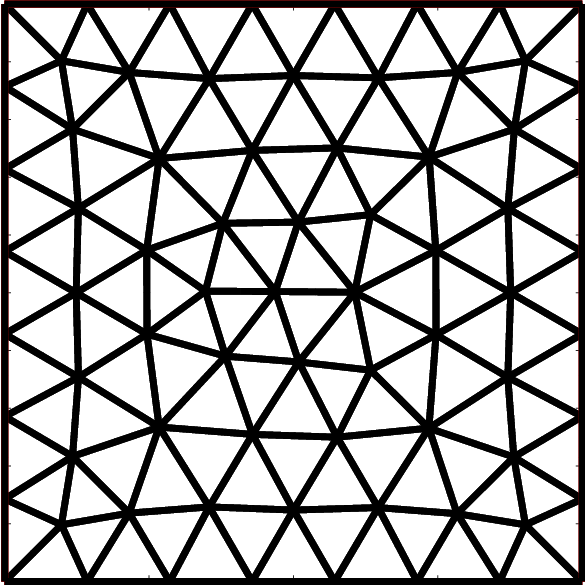
Refer to caption — Figure 1: Illustration of the meshes used for testing the rate of convergence: triangular mesh (left panel), perturbed square mesh (central panel) and Voronoi tesselation (right panel).

6.1 Experimental analysis of the rate of convergence and the divergence free condition.

To assess the performance of the VEM we study the numerical approximations of Problem 4 on a square domain $\Omega=[-1,1]^{2}$ . We consider the velocity field $\bm{u}=(u_{x},u_{y})^{T}$ given by

	$\displaystyle u_{x}(x,y)$	$\displaystyle=-\frac{(x^{2}+y^{2}-1)(\sin(xy)+\cos(xy))-100e^{x}+100e^{y}}{2(50e^{x}-y\sin(xy)+y\cos(xy))},$		(82)
	$\displaystyle u_{y}(x,y)$	$\displaystyle=\frac{(x^{2}+y^{2}-1)(\sin(xy)+\cos(xy))-100e^{x}+100e^{y}}{2(50e^{y}+x\sin(xy)-x\cos(xy))}$		(83)

and the initial and the boundary conditions are set in accordance with the exact solution of the electric and the omagnetic fields:

	$\displaystyle\bm{B}(x,y,t)$	$\displaystyle=\begin{pmatrix}50e^{y}+x\sin(xy)-x\cos(xy)\\[2.5pt] 50e^{x}-y\sin(xy)+y\cos(xy)\end{pmatrix}e^{-t},$		(84)
	$\displaystyle E(x,y,t)$	$\displaystyle=-\big(50(e^{x}-e^{y})+\cos(xy)+\sin(xy)\big)e^{-t}.$		(85)

To check the robustness of the method we have selected three different mesh families, including triangular meshes, randomly perturbed square meshes, and meshes based on Voronoi tessellations. An example of each mesh family is shown in Figure 1.

The time marching scheme uses $\theta=1/2$ . Errors with different values of $\theta$ are very similar and we therefore omit them. The final time is set at $T=0.25$ and the time step follows the assignment $\Delta t=0.05h^{2}$ . Figure 2 shows the log-log plots of the error curves for the approximation of the electric and magnetic fields. The errors are relative and measured in the $L^{2}$ norms, this is to say they are the $L^{2}$ norm of the difference between numerical and exact solutions divided by the norm of the exact solution.

\begin{overpic}[./figures/ElectricTriangularConvergence.eps] \put(0.0,8.5){\begin{sideways}{Electric field relative error}\end{sideways}} \put(40.0,-2.0){{Mesh size $\mathbf{h}$}} \put(17.0,29.0){{2}} \put(26.0,36.0){{1}} \end{overpic}	\begin{overpic}[./figures/MagneticTriangularConvergence.eps] \put(0.0,7.5){\begin{sideways}{Magnetic field relative error}\end{sideways}} \put(40.0,-2.0){{Mesh size $\mathbf{h}$}} \put(17.0,29.0){{1}} \put(25.0,38.0){{1}} \end{overpic}
\begin{overpic}[./figures/ElectricQuadConvergence.eps] \put(0.0,8.5){\begin{sideways}{Electric field relative error}\end{sideways}} \put(40.0,-2.0){{Mesh size $\mathbf{h}$}} \put(16.0,34.0){{2}} \put(25.0,42.0){{1}} \end{overpic}	\begin{overpic}[./figures/MagneticQuadConvergence.eps] \put(0.0,7.5){\begin{sideways}{Magnetic field relative error}\end{sideways}} \put(45.0,-2.0){{Mesh size $\mathbf{h}$}} \put(16.0,25.0){{1}} \put(25.0,32.0){{1}} \end{overpic}
\begin{overpic}[./figures/ElectricVoronoiConvergence.eps] \put(0.0,8.5){\begin{sideways}{Electric field relative error}\end{sideways}} \put(40.0,-2.0){{Mesh size $\mathbf{h}$}} \put(15.0,40.0){{2}} \put(23.0,47.0){{1}} \end{overpic}	\begin{overpic}[./figures/MagneticVoronoiConvergence.eps] \put(0.0,7.5){\begin{sideways}{Magnetic field relative error}\end{sideways}} \put(40.0,-2.0){{Mesh size $\mathbf{h}$}} \put(14.0,25.0){{1}} \put(23.0,33.0){{1}} \end{overpic}

Figure 2: Error curves for the virtual element approximation of the electric and magnetic field (respectively, left and right panels) for the three mesh families of Figure 1: triangular mesh family (top), quadrilateral mesh family (middle), Voronoi mesh family (bottom). The convergence rate is reflected by the slope of the curves in the log-log plots; the reference convergence rate is shown by the triangle in each plot. The symbols E,LS,GI refers to the three alternatives we have for constructing the nodal mass matrix; the elliptic projector (E), least squares projector (LS) and the Galerkin interpolator (GI), respectively.

An important feature of the VEM that we have presented is that the magnetic field remains divergence free throughout the simulations. Next, we will present the results of numerical experiments aimed at gathering experimental evidence to support our theoretical findings. In Figure 3 we present three simulations, each done in a different type of mesh, the $y-$ axis represents the squared $L^{2}$ norm of the magnetic field.

\begin{overpic}[./figures/TriangularDivplot.eps] \put(45.0,-2.0){{\small{Time}}} \put(-6.0,25.0){\begin{sideways}{\small$\|\hskip-0.56905pt\|\hskip-0.56905pt\|\textrm{div}\,\bm{B}_{h}\|\hskip-0.56905pt\|\hskip-0.56905pt\|_{{}_{\mathcal{P}_{h}}}^{2}$}\end{sideways}} \end{overpic}	\begin{overpic}[./figures/QuadDivplot.eps] \put(45.0,-2.0){{\small{Time}}} \put(-6.0,25.0){\begin{sideways}{\small$\|\hskip-0.56905pt\|\hskip-0.56905pt\|\textrm{div}\,\bm{B}_{h}\|\hskip-0.56905pt\|\hskip-0.56905pt\|_{{}_{\mathcal{P}_{h}}}^{2}$}\end{sideways}} \end{overpic}	\begin{overpic}[./figures/VoronoiDivplot.eps] \put(45.0,-2.0){{\small{Time}}} \put(-6.0,25.0){\begin{sideways}{\small$\|\hskip-0.56905pt\|\hskip-0.56905pt\|\textrm{div}\,\bm{B}_{h}\|\hskip-0.56905pt\|\hskip-0.56905pt\|_{{}_{\mathcal{P}_{h}}}^{2}$}\end{sideways}} \end{overpic}

Figure 3: Plots of the time evolution of the square of the

L^{2}

norm of the divergence of the numerical magnetic field on the three mesh families of Figure 1. (Left) triangular mesh, (Middle) quadrilateral cells and (Right) Voronoi tesselation.

6.2 Experimental analysis of the energy estimates

This section is dedicated to an experimental study of the energy estimate presented in Theorem 5.2. For this purpose we define a normalized version of the right hand side and the left hand side of (71) and their difference as:

		$\displaystyle\mathcal{E}_{R}(n)=\frac{\|\hskip-0.56905pt\|\hskip-0.56905pt\|\bm{B}_{h}^{0}\|\hskip-0.56905pt\|\hskip-0.56905pt\|_{{}_{\mathcal{E}_{h}}}^{2}+\gamma\Delta t\sum_{\ell=0}^{n}\beta^{n+1-\ell}\|\hskip-0.56905pt\|\hskip-0.56905pt\|\mathcal{I}^{\mathcal{V}_{h}}E_{0}^{n-\ell+\theta}\|\hskip-0.56905pt\|\hskip-0.56905pt\|_{{}_{H(\textbf{rot};\Omega)}}^{2}}{\|\hskip-0.56905pt\|\hskip-0.56905pt\|\bm{B}_{h}^{0}\|\hskip-0.56905pt\|\hskip-0.56905pt\|_{{}_{\mathcal{E}_{h}}}^{2}},$		(86)
		$\displaystyle\mathcal{E}_{L}(n)=\frac{(\beta)^{n+1}\|\hskip-0.56905pt\|\hskip-0.56905pt\|\bm{B}_{h}^{n+1}\|\hskip-0.56905pt\|\hskip-0.56905pt\|_{{}_{\mathcal{E}_{h}}}^{2}+\frac{\gamma\Delta t}{2}\sum_{\ell=0}^{n}\beta^{n+1-\ell}\|\hskip-0.56905pt\|\hskip-0.56905pt\|\widehat{E}_{h}^{n-\ell+\theta}\|\hskip-0.56905pt\|\hskip-0.56905pt\|_{{}_{\mathcal{V}_{h}}}^{2}}{\|\hskip-0.56905pt\|\hskip-0.56905pt\|\bm{B}_{h}^{0}\|\hskip-0.56905pt\|\hskip-0.56905pt\|_{{}_{\mathcal{E}_{h}}}^{2}},$		(87)
		$\displaystyle\mathcal{E}(n)=\mathcal{E}_{R}(n)-\mathcal{E}_{L}(n).$		(88)

Notice that, by Assumption (73), the value of $\beta$ as defined in (72) is necessarily smaller than $1$ , which implies that most of the coefficients in the terms that appear in $\mathcal{E}$ decay exponentially. Therefore, we can expect that $\mathcal{E}\to 1$ as $n\to\infty$ unless the growth, in time, of the electric and magnetic fields is fast enough to offset this decay. To illustrate this, we introduce a parameter $C\in\mathbbm{R}$ and the family of solutions

	$\displaystyle\bm{B}^{C}(x,y,t)$	$\displaystyle=\begin{pmatrix}50e^{y}-x\sin(xy)+x\cos(xy)\\[2.5pt] 50e^{x}+y\sin(xy)+y\cos(xy)\end{pmatrix}e^{Ct},$		(89)
	$\displaystyle E^{C}(x,y,t)$	$\displaystyle=C\big(50(e^{x}-e^{y})-\cos(xy)-\sin(xy)\big)e^{Ct}$		(90)

and velocity fields $\bm{u}^{C}=(u_{x}^{C},u_{y}^{C})^{T}$ with

	$\displaystyle u_{x}^{C}(x,y)$	$\displaystyle=-C\frac{(-x^{2}-y^{2}-1)(\sin(xy)+\cos(xy))}{2(50e^{x}+y\sin(xy)-y\cos(xy))},$		(91)
	$\displaystyle u_{y}^{C}(x,y)$	$\displaystyle=C\frac{(-x^{2}-y^{2}-1)(\sin(xy)+\cos(xy))}{2(50e^{y}-x\sin(xy)+x\cos(xy))}$		(92)

and define conductivity $\sigma\equiv 1/C$ .

Note that the Assumption (73) yields that any choice of $0<Q<\theta^{-1}$ , as defined in (72), is admissible. In Figure 4 we plot the difference between the right and left hand sides of (71) normalized by the squared $L^{2}$ -norm of the initial condition on the magnetic field against the value of $Q$ at time $T=0.5$ . The type of mesh or the alternative on the nodal mass matrix do not yield significant difference to the results in this figure. Thus, we present the results on Voronoi tessalations of the elliptic projector as a representative with mesh size $h=0.0678$ .

\begin{overpic}[./figures/QvsEnergysmallC.eps] \put(1.0,35.0){\begin{sideways}{$\mathcal{E}$}\end{sideways}} \put(50.0,0.0){{Q}} \end{overpic} \begin{overpic}[./figures/QvsEnergylargeC.eps] \put(1.0,35.0){\begin{sideways}{$\mathcal{E}$}\end{sideways}} \put(50.0,0.0){{Q}} \end{overpic}

Figure 4: Plot of Q against the resulting energy estimate at time

T=0.5

. The initial data that yields the plot in the left is that associated with

C=0.1

and time step

\Delta t=0.001

, whereas the results in the right plot are associated with

C=5

and

\Delta t=0.21

The results of Figure 4 indicate that, in the case that the growth of the solution is relatively small only the values of $Q$ near zero yields $\beta\approx 1$ and the coefficients in $\mathcal{E}$ will show some exponential growth, if $Q\approx\theta^{-1}$ then the value of $\gamma$ blows up yielding that $\mathcal{E}$ will be large. The rest of the values of $Q$ will show convergence towards the norm of the initial conditions on the magnetic field. Since we normalized the error by this value we can expect a flat line of height one. If, however, the solution grows faster than the decay brought about by the coefficients in $\mathcal{E}$ then we will see the energy blow up. Note that the growth in time, at least in our example, of $\mathcal{E}$ is mainly ruled by terms that look like $\beta^{n}e^{Cn\Delta t}$ were $t=n\Delta t$ , hence a rule of thumb for checking whether the energy will grow or flatten is to check if $\ln{\beta}+C\Delta t$ is positive or negative respectively. This is the reason we picked such a small value for $\Delta t$ in the right plot of Figure 4 since large values of $C$ can yield overflow errors. In Figure 5 we can clearly see the two different types of behavior that the energy estimates present.

\begin{overpic}[./figures/EnergyDecay.eps] \put(20.0,-2.0){{Number of Time Steps}} \end{overpic}

\begin{overpic}[./figures/Energygrowth.eps] \put(20.0,-2.0){{Number Of Time Steps}} \end{overpic}

Figure 5: Energy Plots against number of time steps. The initial data that yields the plot in the left is that associated with

C=0.1

and time step

\Delta t=0.001

, whereas the results on the right plot are associated with

C=5

and

\Delta t=0.21

. In both cases,

h=0.0678

6.3 Hartmann Flow

Consider a square duct of infinite length containing a conducting fluid. Assume that this fluid is subjected to a magnetic field that runs along a direction perpendicular to the duct. This is the set up for the Hartmann Flow problem which is regarded as a benchmark in MHD. The behavior of the fluid will depend on the ratio of the Laplace force and the viscous forces, a dimensionless quantity that goes by the name of Hartmann number. There is a set of known formulas that describes the solution to this problem, a proof of which can be found in [44]. It is for this reason that researchers use the Hartmann flow problem to test the performance of their simulations, see e.g. [39, 30, 47].

In this section we consider a square computational domain $[-1,1]^{2}$ as cross section of the aforementioned duct and consider a fluid with conductivity $1$ filling this duct. The magnetic field is applied in the direction of the $y-$ axis. Consider the case where the viscous forces and Laplace forces are of equal strength, so that the Hartmann number is $1$ . Then, we can expect the fluid to behave in accordance to the solution $\bm{B}=(B_{x},1,0)$ , $\bm{u}=(u_{x},0,0)$ and $\bm{E}=(0,0,E_{z})$ with

		$\displaystyle u_{x}(x,y)=\frac{\cosh{1/2}-\cosh{y}}{2\sinh{1/2}},$		(93)
		$\displaystyle B_{x}(x,y)=\frac{\sinh{y}-2y\sinh{1/2}}{2\sinh{1/2}},$
		$\displaystyle E_{z}(x,y)=\frac{2\sinh{1/2}-\cosh{1/2}}{2\sinh{1/2}}\approx-0.0820.$

Note that the $y-$ component of the magnetic field is $1$ by assumption. Therefore, our main interest in this section is in checking if we can recover approximations to the $x-$ component. To do this we feed the analytical solution for the initial and boundary conditions and evolve the system until $T=10$ with step size $\Delta t=0.005$ .

\begin{overpic}[./figures/TopNumericalBx.eps] \put(35.0,-2.0){ { {x -axis} } } \put(-5.0,35.0){ \begin{sideways} {{y-axis}} \end{sideways} } \end{overpic}

\begin{overpic}[./figures/SidewaysExactAndNumerical.eps] \put(45.0,-2.0){{{y-axis}}} \put(-5.0,35.0){\begin{sideways}{{z-axis}}\end{sideways}} \end{overpic}

Figure 6: Plots of the numerical and analytic solutions for the

x-

component of the magnetic field, computed in a Voronoi tesselation of mesh size

h=0.017

using the elliptic projector as the alternative to the mass matrix. The plot on the left is of the numerical solution as viewed from above, whereas the plot on the right shows the numerical solution in a rainbow color bar overlaid with the exact solution in bold black, both are viewed from the side.

The results, to the naked, eye are satisfactory, Figure 6 gives evidence of this fact. We further conducted a convergence test that verifies that every alternative to the mass matrix yields a close approximation and provides additional evidence that rate of convergence of the magnetic field is linear, these results are in Figure 7.

\begin{overpic}[./figures/HMagneticTriangularConvergence.eps] \put(30.0,-2.0){ { \small{Mesh Size h} } } \put(-5.0,15.0){ \begin{sideways} {\small{RelativeError}} \end{sideways} } \put(15.0,28.0){{\small 1}} \put(24.0,35.0){{\small 1}} \end{overpic}	\begin{overpic}[./figures/HMagneticQuadConvergence.eps] \put(30.0,-2.0){{\small{Mesh Size h}}} \put(-5.0,15.0){\begin{sideways}{\small{Relative Error}}\end{sideways}} \put(15.0,40.0){{\small 1}} \put(24.0,46.0){{\small 1}} \end{overpic}	\begin{overpic}[./figures/HMagneticVoronoiConvergence.eps] \put(30.0,-2.0){{\small{Mesh Size h}}} \put(-5.0,15.0){\begin{sideways}{\small{Relative Error}}\end{sideways}} \put(13.5,40.0){{\small 1}} \put(22.0,46.0){{\small 1}} \end{overpic}

Figure 7: Convergence plots for the approximation of the magnetic field on the three different mesh families. The symbols E,LS,GI refers to the three alternatives we have for constructing the nodal mass matrix; the elliptic projector (E), least squares projector (LS) and the Galerkin interpolator (GI) respectively.

7 Conclusions

We developed a virtual element method for the Maxwell system of equations (3) that model the evolution of the electric and magnetic fields of a magnetized fluid whose flow is prescribed. It is well documented that, in order to accurately describe the physics of resistive MHD, it is imperative for the numerical approximation of the magnetic flux field to remain divergence free. This feature is explicitly addressed in this work and Theorem 4.5 rigorously proves that the virtual element scheme in (6) naturally satisfies this requirement. The numerical tests in Section 6 demonstrate that practical implementations of this VEM will satisfy the divergence free condition on the magnetic flux field. Moreover, Theorem 4.1 states that the VEM is wellposed, i.e., that the virtual element approximation exists and is unique. We also proved that the VEM is stable through suitable energy estimates as stated in Theorems 5.1 and 5.2. These estimates were explored numerically in Section 6.

The performance of the method was investigated experimentally, and a set of tests using a manufactured solution and the Hartmann flow problem provide evidence of a quadratic convergence rate for the approximation of electric field and a linear convergence rate for the approximation of the magnetic field.

Future work will focus on the design and implementation of a VEM for (3) in three dimensions and combining such formulation with a flow equation describing the conservation of momentum and mass. We will also introduce a non-linear term into Ohm’s law to describe physical effects related to Hall currents. Such a term is proportional to $\bm{J}\times\bm{B}$ with $\bm{J}=\nabla\times\bm{B}$ as dictated by Ampere’s law. We are also planning to develop a higher order accurate VEM by increasing the order of the local polynomial subspaces, while preserving the commuting de Rham diagram and the free-divergence condition for the magnetic flux field.

Acknowledgements.
S. Naranjo Alvarez’s work was supported by the National Science Foundation (NSF) grant #1545188, “NRT-DESE: Risk and uncertainty quantification in marine science and policy”, which provided a one year fellowship and internship support at Los Alamos National Laboratory. In addition, S. Naranjo Alvarez received graduate research funding from V. A. Bokil’s DMS grant #1720116, an INTERN supplemental award to Professor Bokil’s DMS grant # 1720116 for a second internship at Los Alamos National Laboratory, and teaching support from the Department of Mathematics at Oregon State University.

Professor V. A. Bokil was partially supported by NSF funding from the DMS grant # 1720116. Dr. V. Gyrya and Dr. G. Manzini were supported by the Laboratory Directed Research and Development - Exploratory Research (LDRD-ER) Program of Los Alamos National Laboratory under project number 20180428ER.

The authors would like to thank Dr. K. Lipnikov, T-5 Group, Theoretical Division, Los Alamos National Laboratory, for his advice during the writing of this article. Los Alamos National Laboratory is operated by Triad National Security, LLC, for the National Nuclear Security Administration of U.S. Department of Energy (Contract No. 89233218CNA000001).

References

[1] D. Adak and S. Natarajan. Virtual element method for semilinear Sine-Gordon equation over polygonal mesh using product approximation technique. Mathematics and Computers in Simulation, 172:224–243, 2020.
[2] R. A. Adams and J. J. F. Fournier. Sobolev spaces. Pure and Applied Mathematics. Academic Press, 2 edition, 2003.
[3] B. Ahmad, A. Alsaedi, F. Brezzi, L. D. Marini, and A. Russo. Equivalent projectors for virtual element methods. Computers & Mathematics with Applications, 66:376–391, September 2013.
[4] K. Atkinson and W. Han. Theoretical numerical analysis, volume 39. Springer, 2005.
[5] B. Ayuso de Dios, K. Lipnikov, and G. Manzini. The non-conforming virtual element method. ESAIM: Mathematical Modelling and Numerical Analysis, 50(3):879–904, 2016.
[6] I. Babuska. Error-bounds for finite element method. Numerische Mathematik, 16:322–333, 1970/71.
[7] L. Beirão da Veiga, F. Brezzi, A. Cangiani, G. Manzini, L. D. Marini, and A. Russo. Basic principles of virtual element methods. Mathematical Models & Methods in Applied Sciences, 23:119–214, 2013.
[8] L. Beirão da Veiga, F. Brezzi, F. Dassi, L. D. Marini, and A. Russo. Lowest order virtual element approximation of magnetostatic problems. Computer Methods in Applied Mechanics and Engineering, 332:343–362, 2018.
[9] L. Beirão da Veiga, F. Brezzi, L. D. Marini, and A. Russo. H(div) and H(curl)-conforming VEM. Numerische Mathematik, 133(2):303–332, 2016.
[10] L. Beirão da Veiga, F. Brezzi, L. D. Marini, and A. Russo. Mixed virtual element methods for general second order elliptic problems on polygonal meshes. ESAIM: Mathematical Modelling and Numerical Analysis, 50(3):727–747, 2016.
[11] L. Beirão da Veiga, F. Brezzi, L. D. Marini, and A. Russo. Serendipity nodal vem spaces. Computers and Fluids, 141:2–12, 2016.
[12] L. Beirão da Veiga, F. Brezzi, L. D. Marini, and A. Russo. Virtual element methods for general second order elliptic problems on polygonal meshes. Mathematical Models & Methods in Applied Sciences, 26(4):729–750, 2016.
[13] L. Beirão da Veiga, F. Brezzi, L. D. Marini, and A. Russo. Serendipity face and edge vem spaces. Rend. Lincei Mat. Appl., 28:143–180, 2017.
[14] L. Beirão da Veiga, F. Brezzi, F. Dassi, L. D. Marini, and A. Russo. Virtual element approximation of 2D magnetostatic problems. Computer Methods in Applied Mechanics and Engineering, 327:173–195, 2017.
[15] L. Beirão da Veiga, F. Brezzi, F. Dassi, L. D. Marini, and A. Russo. A family of three-dmensional virtual elements with applications to magnetostatics. SIAM, Journal on Numerical Analysis, 56(5):2940–2962, 2018.
[16] L. Beirão da Veiga, K. Lipnikov, and G. Manzini. Arbitrary order nodal mimetic discretizations of elliptic problems on polygonal meshes. SIAM Journal on Numerical Analysis, 49(5):1737–1760, 2011.
[17] L. Beirão da Veiga, C. Lovadina, and A. Russo. Stability analysis for the virtual element method. Mathematical Models and Methods in Applied Sciences, 27(13):2557–2594, 2017.
[18] L. Beirão da Veiga, G. Manzini, and M. Putti. Post-processing of solution and flux for the nodal mimetic finite difference method. Numerical Methods for Partial Differential Equations, 31(1):336–363, 2015.
[19] S. Berrone, A. Borio, and Manzini. SUPG stabilization for the nonconforming virtual element method for advection–diffusion–reaction equations. Computer Methods in Applied Mechanics and Engineering, 340:500–529, 2018.
[20] D. Boffi, F. Brezzi, and M. Fortin. Mixed finite element methods and applications, volume 44. Springer, 2013.
[21] V. A. Bokil, N. L. Gibson, V. Gyrya, and D. A. McGregor. Dispersion reducing methods for edge discretizations of the electric vector wave equation. Journal of Computational Physics, 287:88–109, 2015.
[22] V. A. Bokil, V. Gyrya, and D. A. McGregor. A dispersion minimized mimetic method for cold plasma. arXiv preprint arXiv:1604.01097, 2016.
[23] J. H. Bramble and S. H. Hilbert. Estimation of linear functionals on Sobolev spaces with application to Fourier transforms and spline interpolation. SIAM Journal on Numerical Analysis, 7:112–124, 1970.
[24] S. C. Brenner and R. Scott. The mathematical theory of finite element methods, volume 15. Springer Science & Business Media, 2008.
[25] S. C. Brenner and L.-Y. Sung. Virtual element methods on meshes with small edges or faces. Mathematical Models and Methods in Applied Sciences, 28(07):1291–1336, 2018.
[26] F. Brezzi, A. Buffa, and K. Lipnikov. Mimetic finite differences for elliptic problems. ESAIM: Mathematical Modelling and Numerical Analysis, 43(2):277–295, 2009.
[27] F. Brezzi, R. S. Falk, and L. D. Marini. Basic principles of mixed virtual element methods. ESAIM. Mathematical Modelling and Numerical Analysis, 48(4):1227–1240, 2014.
[28] A. Cangiani, G. Manzini, and O. Sutton. Conforming and nonconforming virtual element methods for elliptic problems. IMA Journal on Numerical Analysis, 37:1317–1354, 2017. (online August 2016).
[29] L. Chen and J. Huang. Some error analysis on virtual element methods. Calcolo, 55, 2017.
[30] R. Codina and N. Hernández-Silva. Stabilized finite element approximation of the stationary magneto-hydrodynamics equations. Computational Mechanics, 38(4-5):344–355, 2006.
[31] P. Corti. Stable numerical scheme for the magnetic induction equation with hall effect. In Hyperbolic Problems: Theory, Numerics and Applications (In 2 Volumes), pages 374–381. World Scientific, 2012.
[32] R. K. Crockett, P. Colella, R. T. Fisher, R. I. Klein, and C. F. McKee. An unsplit, cell-centered godunov method for ideal mhd. Journal of Computational Physics, 203(2):422–448, 2005.
[33] F. Dassi and L. Mascotto. Exploring high-order three dimensional virtual elements: bases and stabilizations. Comput. Math. Appl., 75(9):3379–3401, 2018.
[34] P. A. Davidson. An introduction to magnetohydrodynamics, 2002.
[35] T. Dupont and R. Scott. Polynomial approximation of functions in Sobolev spaces. Mathematics of Computation, 34(150):441–460, 1980.
[36] . Emmrich. Discrete versions of Gronwall’s lemma and their application to the numerical analysis of parabolic problems, 1999.
[37] V. Gyrya, K. Lipnikov, and G. Manzini. The arbitrary order mixed mimetic finite difference method for the diffusion equation. ESAIM: Mathematical Modelling and Numerical Analysis, 50(3):851–877, 2016.
[38] R. Hiptmair, L. Li, S. Mao, and W. Zheng. A fully divergence-free finite element method for magnetohydrodynamic equations. Mathematical Models and Methods in Applied Sciences, 28(04):659–695, 2018.
[39] K. Hu, Y. Ma, and J. Xu. Stable finite element methods preserving $\nabla\cdot\,{B}=0$ exactly for MHD models. Numerische Mathematik, 135(2):371–396, 2017.
[40] J. M. Hyman and M. Shashkov. Natural discretizations for the divergence, gradient, and curl on logically rectangular grids. Computers & Mathematics with Applications, 33(4):81 – 104, 1997.
[41] K. Lipnikov, G. Manzini, and M. Shashkov. Mimetic finite difference method. Journal of Computational Physics, 257 – Part B:1163–1227, 2014. Review paper.
[42] J.-G. Liu and W.-C. Wang. An energy-preserving MAC–Yee scheme for the incompressible MHD equation. Journal of Computational Physics, 174(1):12–37, 2001.
[43] L. Mascotto. Ill-conditioning in the virtual element method: stabilizations and bases. Numer. Methods Partial Differential Equations, 34(4):1258–1281, 2018.
[44] R. J. Moreau. Magnetohydrodynamics, volume 3. Springer Science & Business Media, 2013.
[45] K. G. Powell, P. L. Roe, T. J. Linde, T. I. Gombosi, and D. L. De Zeeuw. A solution-adaptive upwind scheme for ideal magnetohydrodynamics. Journal of Computational Physics, 154(2):284–309, 1999.
[46] K. Schindler. Physics of space plasma activity. Cambridge University Press, 2006.
[47] J. N. Shadid, R. P. Pawlowski, E. C. Cyr, R. S. Tuminaro, L. Chacón, and P. Weber. Scalable implicit incompressible resistive mhd with stabilized fe and fully-coupled newton–krylov-amg. Computer Methods in Applied Mechanics and Engineering, 304:1–25, 2016.
[48] M. Shashkov. Conservative Finite-Difference Methods on General Grids. Symbolic & Numeric Computation. CRC Press, Francis & Taylor Group, 1995.
[49] M. Shashkov and S. Steinberg. Support-operator finite-difference algorithms for general elliptic problems. Journal of Computational Physics, 118(1):131 – 151, 1995.
[50] M. Torrilhon. Non-uniform convergence of finite volume schemes for Riemann problems of ideal magnetohydrodynamics. Journal of Computational Physics, 192(1):73–94, 2003.
[51] G. Vacca. Virtual element methods for hyperbolic problems on polygonal meshes. Computers & Mathematics with Applications, 74(5):882–898, 2017.

Appendix A Proof of (V3) for $\Pi^{\nabla}_{\textsf{P}}$

We write the elliptic projection of $v_{h}\in\mathcal{V}_{h}(\textsf{P})$ as the linear polynomial $\Pi^{\nabla}_{\textsf{P}}v=\overline{a}+\overline{\bm{b}}\cdot(\bm{x}-\overline{\bm{x}})$ , where

\displaystyle\overline{\bm{x}}=\frac{1}{|\partial\textsf{P}|}\int_{\partial\textsf{P}}\bm{x}dV,\quad\overline{a}=\frac{1}{|\partial\textsf{P}|}\int_{\partial\textsf{P}}v_{h}dS,\quad\overline{\bm{b}}=\frac{1}{|\textsf{P}|}\int_{\textsf{P}}\nabla v_{h}dV,

and $|\partial\textsf{P}|$ is the perimeter of P. A straightforward calculation yields

	$\displaystyle\\|\Pi^{\nabla}_{\textsf{P}}v\\|_{0,\textsf{P}}^{2}$	$\displaystyle=\int_{\textsf{P}}\|\overline{a}+\overline{\bm{b}}\cdot(\bm{x}-\overline{\bm{x}})\|^{2}dV\leq 2\|\overline{a}\|^{2}\|\textsf{P}\|+2\int_{\textsf{P}}\|\overline{\bm{b}}\|^{2}\|\bm{x}-\overline{\bm{x}}\|^{2}dV$
		$\displaystyle\leq 2\|\overline{a}\|^{2}\|\textsf{P}\|+2\|\overline{\bm{b}}\|^{2}\,\int_{\textsf{P}}\|\bm{x}-\overline{\bm{x}}\|^{2}dV\leq 2\|\overline{a}\|^{2}\|\textsf{P}\|+2C\|\overline{\bm{b}}\|^{2}\|\textsf{P}\|h_{\textsf{P}}^{2},$

where $C$ is a “geometric” constant that may depend on the shape of P but does not scale with $h_{\textsf{P}}$ since

\displaystyle\frac{1}{|\textsf{P}|}\int_{\textsf{P}}|\bm{x}-\overline{\bm{x}}|^{2}dV\simeq h_{\textsf{P}}^{2}\mathcal{O}(1).

Then, first using Jensen’s inequality, and, then, Agmon’s inequality yields

	$\displaystyle\|\textsf{P}\|\|\overline{a}\|^{2}$	$\displaystyle=\frac{\|\textsf{P}\|}{\|\partial\textsf{P}\|^{2}}\left\|\int_{\partial\textsf{P}}v_{h}dS\right\|^{2}\leq\frac{\|\textsf{P}\|}{\|\partial\textsf{P}\|^{2}}\,\|\partial\textsf{P}\|\int_{\partial\textsf{P}}\|v_{h}\|^{2}dS\leq\frac{\|\textsf{P}\|}{\|\partial\textsf{P}\|}\int_{\partial\textsf{P}}\|v_{h}\|^{2}dS$
		$\displaystyle\leq\frac{\|\textsf{P}\|}{\|\partial\textsf{P}\|}\,C^{A}\big(h_{\textsf{P}}\|v_{h}\|_{1,\textsf{P}}^{2}+h_{\textsf{P}}^{-1}\\|v_{h}\\|_{0,\textsf{P}}^{2}\big)\leq CC^{A}\left(h_{\textsf{P}}^{2}\|v_{h}\|_{1,\textsf{P}}^{2}+\\|v_{h}\\|_{0,\textsf{P}}^{2}\right),$

where $C^{A}$ is the constant of Agmon’s inequality. In the above inequality we used the fact $|\textsf{P}|h_{\textsf{P}}/\penalty{{|\partial\textsf{P}|}}=\mathcal{O}\big(h_{\textsf{P}}^{2}\big)$ and $|\textsf{P}|h_{\textsf{P}}^{-1}/\penalty{{|\partial\textsf{P}|}}=\mathcal{O}(1)$ since $h_{\textsf{P}}/\penalty{|\partial\textsf{P}|}$ and $|\textsf{P}|/\penalty{h_{\textsf{P}}^{2}}$ are uniformly bounded quantities in view of Assumption (M2). This assumption also implies that the real positive constant $C$ may only depend on $\rho$ , and, from Agmon’s inequality, on the number of polygonal edges, this latter also being uniformly bounded. Using again Jensen’s inequality yields

\displaystyle|\textsf{P}|h_{\textsf{P}}^{2}|\overline{\bm{b}}|^{2}=\frac{|\textsf{P}|h_{\textsf{P}}^{2}}{|\textsf{P}|^{2}}\left|\int_{\textsf{P}}\nabla v_{h}dV\right|^{2}=\frac{|\textsf{P}|h_{\textsf{P}}^{2}}{|\textsf{P}|^{2}}\,|\textsf{P}|\int_{\textsf{P}}|\nabla v_{h}|^{2}dV\leq h_{\textsf{P}}^{2}\int_{\textsf{P}}|\nabla v_{h}|^{2}dV=h_{\textsf{P}}^{2}|v_{h}|_{1,\textsf{P}}^{2}.

Finally, we collect the estimates for $|\textsf{P}||\overline{a}|^{2}$ and $|\textsf{P}|h_{\textsf{P}}^{2}|\overline{\bm{b}}|^{2}$ , and apply the inverse inequality

\displaystyle|v_{h}|_{1,\textsf{P}}\leq C^{I}h_{\textsf{P}}^{-1}\|v_{h}\|_{0,\textsf{P}},

(94)

which follows from a scaling argument, see [20, Chapter 2] and the recent work of Ref. [29], and whose constant $C^{I}$ is independent of $h_{\textsf{P}}$ to obtain:

\displaystyle\|\Pi^{\nabla}_{\textsf{P}}v\|_{0,\textsf{P}}^{2}\leq C\left(h_{\textsf{P}}^{2}|v_{h}|_{1,\textsf{P}}^{2}+\|v_{h}\|_{0,\textsf{P}}^{2}\right)\leq C\left(C^{I}h_{\textsf{P}}^{2}h_{\textsf{P}}^{-2}\|v_{h}\|_{0,\textsf{P}}^{2}+\|v_{h}\|_{0,\textsf{P}}^{2}\right)\leq C\|v_{h}\|_{0,\textsf{P}}^{2}.

Tracing back the constants introduced in the various inequalities, we find that the final constant $C$ may depend on $C^{A}$ , $C^{I}$ , $\rho$ , but is independent of $h_{\textsf{P}}$ , and is obviously the same for all $v_{h}\in\mathcal{V}_{h}(\textsf{P})$ . This argument provides the desired upper bound on operator $\Pi^{\nabla}_{\textsf{P}}$ .

Appendix B Proof of (V3) for $\Pi^{LS}_{\textsf{P}}$

The Least Squares reconstruction operator applied to $v_{h}\in\mathcal{V}_{h}(\textsf{P})$ provides the linear polynomial (22), which we conveniently rewrite here:

\displaystyle\Pi^{LS}_{\textsf{P}}v_{h}(x,y)=a+b\frac{x-x_{\textsf{P}}}{h_{\textsf{P}}}+c\frac{y-y_{\textsf{P}}}{h_{\textsf{P}}}.

(95)

The three coefficients $a$ , $b$ and $c$ are determined by imposing the conditions in (23). Let $\bm{\zeta}=(a,b,c)^{T}$ denote the vector collecting the three unknowns in (95). Let $\bm{x}_{\textsf{v}_{i}}=(x_{\textsf{v}_{i}},y_{\textsf{v}_{i}})^{T}$ denote the coordinate vector of the $i$ -th vertex $\textsf{v}_{i}$ for $i=1,2,\ldots,N^{\mathcal{V}}$ , $N^{\mathcal{V}}$ being the number of vertices of P, and $\bm{\eta}=\big(v_{h}(\bm{x}_{\textsf{v}_{1}}),v_{h}(\bm{x}_{\textsf{v}_{2}}),\ldots,v_{h}(\bm{x}_{\textsf{v}_{N^{\mathcal{V}}}})\big)^{T}$ the vector collecting the nodal degrees of freedom of $v_{h}$ . Using this notation, we rewrite the linear system (23) in the more compact form $\mathbbm{A}\bm{\zeta}=\bm{\eta}$ , where the matrix of the system coefficients is given by:

\displaystyle\mathbbm{A}=\left[\begin{array}[]{cc}1&\quad\dfrac{(\bm{x}_{\textsf{v}_{1}}-\bm{x}_{\textsf{P}})^{T}}{h_{\textsf{P}}}\\[5.0pt] 1&\quad\dfrac{(\bm{x}_{\textsf{v}_{2}}-\bm{x}_{\textsf{P}})^{T}}{h_{\textsf{P}}}\\[5.0pt] \vdots&\vdots\\[5.0pt] 1&\quad\dfrac{(\bm{x}_{\textsf{v}_{N^{\mathcal{V}}}}-\bm{x}_{\textsf{P}})^{T}}{h_{\textsf{P}}}\end{array}\right]=\left[\begin{array}[]{ccc}1&\quad\dfrac{x_{\textsf{v}_{1}}-x_{\textsf{P}}}{h_{\textsf{P}}}&\quad\dfrac{y_{\textsf{v}_{1}}-y_{\textsf{P}}}{h_{\textsf{P}}}\\[5.0pt] 1&\quad\dfrac{x_{\textsf{v}_{2}}-x_{\textsf{P}}}{h_{\textsf{P}}}&\quad\dfrac{y_{\textsf{v}_{2}}-y_{\textsf{P}}}{h_{\textsf{P}}}\\[5.0pt] \vdots&\vdots&\vdots\\[5.0pt] 1&\quad\dfrac{x_{\textsf{v}_{N^{\mathcal{V}}}}-x_{\textsf{P}}}{h_{\textsf{P}}}&\quad\dfrac{y_{\textsf{v}_{N^{\mathcal{V}}}}-y_{\textsf{P}}}{h_{\textsf{P}}}\end{array}\right].

The coefficients of the least squares solution are given by solving the normal equations, i.e., $\bm{\zeta}=(\mathbbm{A}^{T}\mathbbm{A})^{-1}\mathbbm{A}^{T}\bm{\eta}$ .

Now, we introduce the discrete norm

\displaystyle|\hskip-0.56905pt|\hskip-0.56905pt|v_{h}|\hskip-0.56905pt|\hskip-0.56905pt|_{{}_{\textsf{P}}}^{2}=|\textsf{P}|\sum_{i=1}^{N^{\mathcal{V}}}|v_{h}(\bm{x}_{\textsf{v}_{i}})|^{2}=|\textsf{P}|\big|\bm{\eta}\big|^{2}

(96)

and we observe that

\displaystyle|\hskip-0.56905pt|\hskip-0.56905pt|\Pi^{LS}_{\textsf{P}}v_{h}|\hskip-0.56905pt|\hskip-0.56905pt|_{{}_{\textsf{P}}}^{2}=|\textsf{P}|\sum_{i=1}^{N^{\mathcal{V}}}\big|\Pi^{LS}_{\textsf{P}}v_{h}(\bm{x}_{\textsf{v}_{i}})\big|^{2}=|\textsf{P}|\sum_{i=1}^{N^{\mathcal{V}}}\Big|a+b\frac{x_{\textsf{v}_{i}}-x_{\textsf{P}}}{h_{\textsf{P}}}+c\frac{y_{\textsf{v}_{i}}-y_{\textsf{P}}}{h_{\textsf{P}}}\Big|^{2}=|\textsf{P}|\big|\mathbbm{A}\bm{\zeta}\big|^{2}.

(97)

The norm defined in (96) is spectrally equivalent to the $L^{2}$ norm, so that there exist two strictly positive constant $\nu_{*}$ and $\nu^{*}$ such that

\displaystyle\nu_{*}\|v_{h}\|_{0,\textsf{P}}\leq|\hskip-0.56905pt|\hskip-0.56905pt|v_{h}|\hskip-0.56905pt|\hskip-0.56905pt|_{{}_{\textsf{P}}}\leq\nu^{*}\|v_{h}\|_{0,\textsf{P}}\quad\forall v_{h}\in\mathcal{V}_{h}(\textsf{P}).

(98)

The two norms $\|v_{h}\|_{0,\textsf{P}}$ and $|\hskip-0.56905pt|\hskip-0.56905pt|v_{h}|\hskip-0.56905pt|\hskip-0.56905pt|_{{}_{\textsf{P}}}$ , because of the explicit dependence of the latter on $|\textsf{P}|$ , have the same scaling with respect to $h_{\textsf{P}}$ . Therefore, the two constants $\nu_{*}$ and $\nu^{*}$ may depend on the geometric shape of P but must be independent of $h_{\textsf{P}}$ .

A straightforward calculation starting from the left inequality of (98) yields

\displaystyle\begin{array}[]{rll}\|\Pi^{LS}_{\textsf{P}}v\|_{0,\textsf{P}}&\leq(\nu_{*})^{-1}|\hskip-0.56905pt|\hskip-0.56905pt|\Pi^{LS}_{\textsf{P}}v_{h}|\hskip-0.56905pt|\hskip-0.56905pt|_{{}_{\textsf{P}}}&\hskip 28.45274pt\mbox{\big[use~\eqref{app:eq:discrete:norm:10}\big]}\\[5.0pt] &=(\nu_{*})^{-1}|\textsf{P}|^{\frac{1}{2}}\big|\mathbbm{A}\bm{\zeta}\big|&\hskip 28.45274pt\mbox{\big[substitute~$\bm{\zeta}=\big(\mathbbm{A}^{T}\mathbbm{A}\big)^{-1}\mathbbm{A}^{T}\bm{\eta}$\big]}\\[5.0pt] &=(\nu_{*})^{-1}|\textsf{P}|^{\frac{1}{2}}\big|\mathbbm{A}\big(\mathbbm{A}^{T}\mathbbm{A}\big)^{-1}\mathbbm{A}^{T}\bm{\eta}\big|&\hskip 28.45274pt\mbox{\big[use the continuity of $\mathbbm{A}\big(\mathbbm{A}^{T}\mathbbm{A}\big)^{-1}\mathbbm{A}^{T}$\big]}\\[5.0pt] &\leq(\nu_{*})^{-1}|\textsf{P}|^{\frac{1}{2}}\big|\mathbbm{A}\big(\mathbbm{A}^{T}\mathbbm{A}\big)^{-1}\mathbbm{A}^{T}\big||\bm{\eta}|&\hskip 28.45274pt\mbox{\big[note that $\mathbbm{A}\big(\mathbbm{A}^{T}\mathbbm{A}\big)^{-1}\mathbbm{A}^{T}$ is a projector\big]}\\[5.0pt] &\leq(\nu_{*})^{-1}|\textsf{P}|^{\frac{1}{2}}\big|\bm{\eta}\big|&\hskip 28.45274pt\mbox{\big[use~\eqref{app:eq:discrete:norm}\big]}\\[5.0pt] &=(\nu_{*})^{-1}|\hskip-0.56905pt|\hskip-0.56905pt|v_{h}|\hskip-0.56905pt|\hskip-0.56905pt|_{{}_{\textsf{P}}}&\hskip 28.45274pt\mbox{\big[use the right inequality of~\eqref{app:eq:norm:equivalence}\big]}\\[5.0pt] &\leq\frac{\nu^{*}}{\nu_{*}}\|v_{h}\|_{0,\textsf{P}}.\end{array}

In the chain of inequalities above, we used the fact that $\mathbbm{A}\big(\mathbbm{A}^{T}\mathbbm{A}\big)^{-1}\mathbbm{A}^{T}$ is the orthogonal projection operator with respect to the Euclidean inner product onto the span of the columns of matrix $\mathbbm{A}$ . This projection operator scales like $\mathcal{O}(1)$ with respect to $h_{\textsf{P}}$ by definition of matrix $\mathbbm{A}$ , and its eigenvalues must be $0$ and $1$ . As a consequence, it is continuous and such that $|\mathbbm{A}\big(\mathbbm{A}^{T}\mathbbm{A})^{-1}\mathbbm{A}^{T}|=1$ . Finally, we note that in this case the constant $C$ that appears in the assertion of proposition (V3) is equal to $(\nu^{*}/\penalty{\nu_{*}})$ , and is independent of $h$ as already pointed out above.

$\displaystyle\|\hskip-0.56905pt\|\hskip-0.56905pt\|\mathcal{I}^{\mathcal{V}_{h}}v\|\hskip-0.56905pt\|\hskip-0.56905pt\|_{{}_{\mathcal{V}_{h}}}$	$\displaystyle\!\leq C\\|v\\|_{0,\Omega}\phantom{\\|\bm{w}\\|_{0,\Omega}\\|v\\|_{0,\Omega}}\hskip-42.67912pt\forall v\in H^{1}(\Omega),$	(35)
$\displaystyle\|\hskip-0.56905pt\|\hskip-0.56905pt\|\mathcal{I}^{\mathcal{E}_{h}}\bm{w}\|\hskip-0.56905pt\|\hskip-0.56905pt\|_{{}_{\mathcal{E}_{h}}}$	$\displaystyle\!\leq C\\|\bm{w}\\|_{0,\Omega}\phantom{\\|v\\|_{0,\Omega}\\|v\\|_{0,\Omega}}\hskip-42.67912pt\forall\bm{w}\in V,$	(36)
$\displaystyle\|\hskip-0.56905pt\|\hskip-0.56905pt\|\mathcal{I}^{\mathcal{P}_{h}}v\|\hskip-0.56905pt\|\hskip-0.56905pt\|_{{}_{\mathcal{P}_{h}}}$	$\displaystyle\!\leq C\\|v\\|_{0,\Omega}\phantom{\\|v\\|_{0,\Omega}\\|\bm{w}\\|_{0,\Omega}}\hskip-42.67912pt\forall v\in L^{2}(\Omega).$	(37)

	$\displaystyle\|\hskip-0.56905pt\|\hskip-0.56905pt\|\eta_{\xi}\|\hskip-0.56905pt\|\hskip-0.56905pt\|_{{}_{\mathcal{X}_{h}}}^{2}$	$\displaystyle=\|\hskip-0.56905pt\|\hskip-0.56905pt\|(\theta/\penalty{2})\,\big(\bm{B}_{h}+\Delta t\ \textbf{rot}\,E_{h}\big)\|\hskip-0.56905pt\|\hskip-0.56905pt\|_{{}_{\Delta t,\textrm{div}\,}}^{2}+\|\hskip-0.56905pt\|\hskip-0.56905pt\|E_{h}\|\hskip-0.56905pt\|\hskip-0.56905pt\|_{{}_{\Delta t,\textbf{rot}\,}}^{2}$
		$\displaystyle=\frac{\theta^{2}}{4}\left(\Delta t^{-1}\|\hskip-0.56905pt\|\hskip-0.56905pt\|\bm{B}_{h}+\Delta t\textbf{rot}\,E_{h}\|\hskip-0.56905pt\|\hskip-0.56905pt\|_{{}_{\mathcal{E}_{h}}}^{2}+\\|\textrm{div}\,\bm{B}_{h}\\|_{0,\Omega}^{2}\right)+\|\hskip-0.56905pt\|\hskip-0.56905pt\|E_{h}\|\hskip-0.56905pt\|\hskip-0.56905pt\|_{{}_{\Delta t,\textbf{rot}\,}}^{2}$
		$\displaystyle=\frac{\theta^{2}}{4}\left(\Delta t^{-1}\|\hskip-0.56905pt\|\hskip-0.56905pt\|\bm{B}_{h}\|\hskip-0.56905pt\|\hskip-0.56905pt\|_{{}_{\mathcal{E}_{h}}}^{2}+\Delta t\|\hskip-0.56905pt\|\hskip-0.56905pt\|\textbf{rot}\,E_{h}\|\hskip-0.56905pt\|\hskip-0.56905pt\|_{{}_{\mathcal{E}_{h}}}^{2}+2\Big(\bm{B}_{h},\textbf{rot}\,E_{h}\Big)_{\mathcal{E}_{h}}+\\|\textrm{div}\,\bm{B}_{h}\\|_{0,\Omega}^{2}\right)+\|\hskip-0.56905pt\|\hskip-0.56905pt\|E_{h}\|\hskip-0.56905pt\|\hskip-0.56905pt\|_{{}_{\Delta t,\textbf{rot}\,}}^{2}$
		$\displaystyle=\frac{\theta^{2}}{4}\left(\Delta t^{-1}\|\hskip-0.56905pt\|\hskip-0.56905pt\|\bm{B}_{h}\|\hskip-0.56905pt\|\hskip-0.56905pt\|_{{}_{\mathcal{E}_{h}}}^{2}\hskip-2.84526pt+\hskip-2.84526pt\\|\textrm{div}\,\bm{B}_{h}\\|_{0,\Omega}^{2}\hskip-2.84526pt+\hskip-2.84526pt2\Big(\Delta t^{-1/2}\bm{B}_{h},\Delta t^{1/2}\textbf{rot}\,E_{h}\Big)_{\mathcal{E}_{h}}\hskip-2.84526pt+\hskip-2.84526pt\Delta t\|\hskip-0.56905pt\|\hskip-0.56905pt\|\textbf{rot}\,E_{h}\|\hskip-0.56905pt\|\hskip-0.56905pt\|_{{}_{\mathcal{E}_{h}}}^{2}\right)+\|\hskip-0.56905pt\|\hskip-0.56905pt\|E_{h}\|\hskip-0.56905pt\|\hskip-0.56905pt\|_{{}_{\Delta t,\textbf{rot}\,}}^{2}$
		$\displaystyle\leq\frac{\theta^{2}}{4}\left(2\Delta t^{-1}\|\hskip-0.56905pt\|\hskip-0.56905pt\|\bm{B}_{h}\|\hskip-0.56905pt\|\hskip-0.56905pt\|_{{}_{\mathcal{E}_{h}}}^{2}+\\|\textrm{div}\,\bm{B}_{h}\\|_{0,\Omega}^{2}+2\Delta t\|\hskip-0.56905pt\|\hskip-0.56905pt\|\textbf{rot}\,E_{h}\|\hskip-0.56905pt\|\hskip-0.56905pt\|_{{}_{\mathcal{E}_{h}}}^{2}\right)+\|\hskip-0.56905pt\|\hskip-0.56905pt\|E_{h}\|\hskip-0.56905pt\|\hskip-0.56905pt\|_{{}_{\Delta t,\textbf{rot}\,}}^{2}$
		$\displaystyle\leq\frac{\theta^{2}}{2}\|\hskip-0.56905pt\|\hskip-0.56905pt\|\bm{B}_{h}\|\hskip-0.56905pt\|\hskip-0.56905pt\|_{{}_{\Delta t,\textrm{div}\,}}^{2}+\left(1+\frac{\theta^{2}}{2}\right)\|\hskip-0.56905pt\|\hskip-0.56905pt\|E_{h}\|\hskip-0.56905pt\|\hskip-0.56905pt\|_{{}_{\Delta t,\textbf{rot}\,}}^{2}$
		$\displaystyle\leq\left(1+\frac{\theta^{2}}{2}\right)\|\hskip-0.56905pt\|\hskip-0.56905pt\|\xi\|\hskip-0.56905pt\|\hskip-0.56905pt\|_{{}_{\mathcal{X}_{h}}}^{2}.$

	$\displaystyle\|\hskip-0.56905pt\|\hskip-0.56905pt\|\mathcal{I}^{\mathcal{V}_{h}}(\bm{u}\times\Pi^{RT}\bm{B}_{h}^{n+\theta})\|\hskip-0.56905pt\|\hskip-0.56905pt\|_{{}_{\mathcal{V}_{h}}}^{2}$	$\displaystyle\leq C\\|\bm{u}\\|_{\infty}^{2}\|\hskip-0.56905pt\|\hskip-0.56905pt\|\theta\bm{B}_{h}^{n+1}+(1-\theta)\bm{B}_{h}^{n}\|\hskip-0.56905pt\|\hskip-0.56905pt\|_{{}_{\mathcal{E}_{h}}}^{2}$
		$\displaystyle\leq 2C\\|\bm{u}\\|_{\infty}^{2}\left(\theta^{2}\|\hskip-0.56905pt\|\hskip-0.56905pt\|\bm{B}_{h}^{n+1}\|\hskip-0.56905pt\|\hskip-0.56905pt\|_{{}_{\mathcal{E}_{h}}}^{2}+(1-\theta)^{2}\|\hskip-0.56905pt\|\hskip-0.56905pt\|\bm{B}_{h}^{n}\|\hskip-0.56905pt\|\hskip-0.56905pt\|_{{}_{\mathcal{E}_{h}}}^{2}\right)$
		$\displaystyle\leq 2C\\|\bm{u}\\|_{\infty}^{2}\left(\theta\|\hskip-0.56905pt\|\hskip-0.56905pt\|\bm{B}_{h}^{n+1}\|\hskip-0.56905pt\|\hskip-0.56905pt\|_{{}_{\mathcal{E}_{h}}}^{2}+(1-\theta)\|\hskip-0.56905pt\|\hskip-0.56905pt\|\bm{B}_{h}^{n}\|\hskip-0.56905pt\|\hskip-0.56905pt\|_{{}_{\mathcal{E}_{h}}}^{2}\right).$

	$\displaystyle\|\hskip-0.56905pt\|\hskip-0.56905pt\|\bm{B}_{h}^{n+1}\|\hskip-0.56905pt\|\hskip-0.56905pt\|_{{}_{\mathcal{E}_{h}}}^{2}-\|\hskip-0.56905pt\|\hskip-0.56905pt\|\bm{B}_{h}^{n}\|\hskip-0.56905pt\|\hskip-0.56905pt\|_{{}_{\mathcal{E}_{h}}}^{2}$	$\displaystyle\leq\Delta t\left(-\frac{1}{2}\|\hskip-0.56905pt\|\hskip-0.56905pt\|\widehat{E}_{h}^{n+\theta}\|\hskip-0.56905pt\|\hskip-0.56905pt\|_{{}_{\mathcal{V}_{h}}}^{2}+\|\hskip-0.56905pt\|\hskip-0.56905pt\|\mathcal{I}^{\mathcal{V}_{h}}E_{0}^{n+\theta}\|\hskip-0.56905pt\|\hskip-0.56905pt\|_{{}_{H(\textbf{rot};\Omega)}}^{2}\right)$
		$\displaystyle\qquad+\Delta t\big(1+4\widetilde{C}\\|\bm{u}\\|_{\infty}^{2}\big)\,\left(\theta\|\hskip-0.56905pt\|\hskip-0.56905pt\|\bm{B}_{h}^{n+1}\|\hskip-0.56905pt\|\hskip-0.56905pt\|_{{}_{\mathcal{E}_{h}}}^{2}+(1-\theta)\|\hskip-0.56905pt\|\hskip-0.56905pt\|\bm{B}_{h}^{n}\|\hskip-0.56905pt\|\hskip-0.56905pt\|_{{}_{\mathcal{E}_{h}}}^{2}\right).$		(80)

The virtual element method for resistive magnetohydrodynamics.

Abstract

1 Introduction

1.1 Notation, functional spaces and technicalities

2 The mathematical formulation

3 The virtual element method

3.1 Assumptions on mesh regularity

3.2 Nodal virtual element space

Remark 3.1

3.2.1 Properties of the inner product (12)

Lemma 3.2

Remark 3.3

3.2.2 Construction of operator ΠP𝒱h\Pi^{\mathcal{V}_{h}}_{\textsf{P}}

3.3 Edge virtual element space

3.4 Cell space

3.5 Interpolation operators and approximation of (σ​𝒖×𝑩,v)\big(\sigma\bm{u}\times\bm{B},v\big)

Lemma 3.4

3.6 Commuting properties and the virtual De-Rham complex

Lemma 3.5 (Commutation properties)

Theorem 3.6

4 Wellposedness of the Virtual Element Method

Theorem 4.1

Problem 4.2

4.1 Abstract setting and equivalent problems

Problem 4.3

Problem 4.4

Theorem 4.5 (Zero-divergence magnetic flux from system (6))

Theorem 4.6 (Zero-divergence magnetic flux from Problem 4.4)

Theorem 4.7 (Equivalence of Problems 4.2, 4.3, and 4.4)

Lemma 4.8

Lemma 4.9

5 Stability energy estimates

Theorem 5.1

Theorem 5.2

Remark 5.3

6 Numerical experiments

6.1 Experimental analysis of the rate of convergence and the divergence free condition.

6.2 Experimental analysis of the energy estimates

6.3 Hartmann Flow

7 Conclusions

References

Appendix A Proof of (V3) for ΠP∇\Pi^{\nabla}_{\textsf{P}}

Appendix B Proof of (V3) for ΠPL​S\Pi^{LS}_{\textsf{P}}

3.2.2 Construction of operator $\Pi^{\mathcal{V}_{h}}_{\textsf{P}}$

3.5 Interpolation operators and approximation of $\big(\sigma\bm{u}\times\bm{B},v\big)$

Appendix A Proof of (V3) for $\Pi^{\nabla}_{\textsf{P}}$

Appendix B Proof of (V3) for $\Pi^{LS}_{\textsf{P}}$