DAYENU: A Simple Filter of Smooth Foregrounds for Intensity Mapping Power Spectra2019DAYENU: A Simple Filter of Smooth Foregrounds for Intensity Mapping Power Spectra–17

The data ${\bf x}$ observed in a fluctuation experiment can be decomposed into foregrounds ($\boldsymbol{f}$), noise ($\boldsymbol{n}$), and cosmological fluctuations ($\boldsymbol{s}$).

Since $\boldsymbol{f}$, $\boldsymbol{n}$, and $\boldsymbol{s}$ are independent, $\boldsymbol{\mathsf{C}}=\langle{\bf x}{\bf x}^{\dagger}\rangle-\langle{\bf x}\rangle\langle{\bf x}^{\dagger}\rangle$ can be decomposed into

where $\boldsymbol{\mathsf{N}}=\langle\boldsymbol{n}\boldsymbol{n}^{\dagger}\rangle$, $\boldsymbol{\mathsf{S}}=\langle\boldsymbol{s}\boldsymbol{s}^{\dagger}\rangle-\langle\boldsymbol{s}\rangle\langle\boldsymbol{s}^{\dagger}\rangle$, and $\boldsymbol{\mathsf{C}}_{\text{fg}}=\langle\boldsymbol{f}\boldsymbol{f}^{\dagger}\rangle-\langle\boldsymbol{f}\rangle\langle\boldsymbol{f}^{\dagger}\rangle$.

Bandpowers are usually defined by decomposing $\boldsymbol{\mathsf{S}}$ into a set of response matrices

While many authors stick with bandpowers that only describe $\boldsymbol{\mathsf{S}}$, Parsons et al. 2014; Ali et al. 2015; Liu et al. 2014a; Liu et al. 2014b adopt bandpower definitions where $\boldsymbol{\mathsf{C}}_{\text{fg}}+\boldsymbol{\mathsf{S}}=\sum_{\alpha}p^{\alpha}\boldsymbol{{\mathsf{C}_{,\alpha}}}$. The decision to define bandpowers for the signal covariance $\boldsymbol{\mathsf{S}}$ alone versus $\boldsymbol{\mathsf{C}}_{\text{fg}}+\boldsymbol{\mathsf{S}}$ is an analysis choice with important consequences that we explore in paper II. Since we do not know the 21 cm signal a-priori, we don’t actually know what the correct bandpowers to use are. Instead, we choose a set of response matrices $\boldsymbol{{\widehat{\mathsf{C}}_{,\alpha}}}$ that may not actually be correct. A standard choice for $\boldsymbol{{\widehat{\mathsf{C}}_{,\alpha}}}$ uses our expectation that the 21 cm signal is homogenous so that the correlation between temperatures at two locations is given by the continuous Fourier transform of the power-spectrum. Authors usually replace this continuous Fourier Transform with a DFT. Thus, many works (e.g. (Dillon et al. 2015; Trott et al. 2016; Barry et al. 2019; Mertens et al. 2020)) choose $\boldsymbol{{\widehat{\mathsf{C}}_{,\alpha}}}=\boldsymbol{{\mathsf{C}_{,\alpha}}}^{\text{\bf DFT}}$. For a three-dimensional data-cube, each data-point $x_{m}$ has an associated co-moving position ${\bf r_{m}}$ so

where $V_{\alpha}$ are fourier-space bins (cylindrical or spherical) and ${\bf k}$ are wave-numbers given by the DFT of a gridded image.

In this work, we focus on per-baseline QEs employed by PAPER and HERA (Parsons et al. 2012b; Parsons et al. 2014; Ali et al. 2015) which operate independently on different baselines at different LSTs. These estimators sacrifice a small amount of sensitivity for short baselines (Zhang et al. 2018) and have the advantage of being analytically and computationally simple to work with. For a per-baseline estimator, ${\bf x}$ is the frequency data from a single visibility at a single LST that has potentially been averaged over many identical copies in a redundant baseline group and many different nights at the same LST. We emphasize that this estimator is distinctive from a multi-baseline estimator where the data are ${\bf x}$ consists of all baselines in our data set (e.g. Liu et al. 2014a; Liu et al. 2014b). The DFT bandpowers used in per-baseline estimators are usually just the squared coefficients of a 1D frequency DFT. If the baselines are all sufficiently close together, each spherical $k$-bin is the same as each $k_{\parallel}$ bin in the LoS DFT. Parsons et al. 2014, Ali et al. 2015, and in this paper, we focus on LoS DFT bandpowers

In the QE formalism, we denote our $N_{\text{b}}$ estimates of bandpowers $\hat{p}_{\alpha}$ to be equal to a normalized linear combination pairwise multiplications of data points,

where $\boldsymbol{\mathsf{E}_{\beta}}$ is one of $N_{\text{b}}$ different $N_{\text{d}}\times N_{\text{d}}$ matrices (one for each bandpower) that perform a weighted sum over pairs of data measurements. $\boldsymbol{\mathsf{M}}$ is an $N_{\text{b}}\times N_{\text{b}}$ normalization matrix and $\hat{b}_{\alpha}$ is a subtracted estimate of the true bias $b_{\alpha}$ which includes all covariance contributions not described by bandpowers.

It is convenient to expand $\boldsymbol{\mathsf{E}_{\alpha}}$ into a product of filter matrices, $\boldsymbol{\mathsf{R}}$, and a quadratic matrix, $\boldsymbol{\mathsf{Q}_{\alpha}}$:

Under this expansion, $\boldsymbol{\mathsf{R}}$ describes all filtering applied to data prior to Fourier transforming. For a single visibility, this could be the apodization by a Blackman-Harris window in which case $\mathsf{R}^{\text{BH}}_{mn}\equiv\delta_{mn}^{k}T_{n}^{\text{BH}}$, where $\boldsymbol{\delta^{k}}$ is the Kronecker delta matrix and $T_{n}^{\text{BH}}$ is the $n^{\mathrm{th}}$ element of a Blackman-Harris window. Alternatively, for inverse covariance weighting, we might set $\boldsymbol{\mathsf{R}}^{\text{OQE}}\equiv\boldsymbol{\mathsf{C}}^{-1}$. $\boldsymbol{\mathsf{Q}_{\alpha}}$ performs the transformation into the bandpower basis for both data vectors along with binning and squaring. A standard example for $\boldsymbol{\mathsf{Q}_{\alpha}}$ used to estimate DFT bandpowers is the per-baseline delay-transform matrix

$\boldsymbol{\mathsf{M}}$ is usually chosen in a way that trades off mixing between band-powers and their error correlations. The expectation value of each estimated bandpower, $\hat{p}^{\alpha}$ is equal to an admixture of true bandpowers

where

and

The optimal quadratic estimator that minimizes error bars and preserves all information from the original data is given by (Tegmark 1997; Liu & Tegmark 2011),

where $\text{Diag}(\boldsymbol{\mathsf{F}})$ is the diagonal of the Fisher information matrix given by

If we instead choose, $\boldsymbol{\mathsf{M}}=\boldsymbol{\mathsf{F}}^{-1}$, $\hat{p}_{\text{OQE}}$ also has the desirable property that its window functions are Kronecker deltas so that no mixing between bandpowers occurs. However, fluctuations from the mean, described by the bandpower covariance matrix

are significantly larger and more correlated (Liu & Tegmark 2011).

Comparing equation (16) with equations (9) and (11), one can plainly see that the OQE is a result of choosing $\boldsymbol{\mathsf{R}}^{\text{\bf OQE}}=\boldsymbol{\mathsf{C}}^{-1}$, $\boldsymbol{\mathsf{Q}_{\alpha}}^{\text{\bf OQE}}=\boldsymbol{{\mathsf{C}_{,\alpha}}}$.

Before we construct a simple covariance filter, we should get a sense of what the requirements on an inverse covariance filter are by writing down its action on a data vector.

If $\boldsymbol{\mathsf{Q}_{\alpha}}$ performs an untapered Fourier transform, then any foregrounds that are left in our data at this point will be smeared by RFI gaps and the finite bandwidth. Thus, we want the ratio between foregrounds and signal in our inverse covariance-weighted data to be smaller then the level of side-lobes from finite bandwidth and RFI gaps.

To see what requirements this demand puts on our covariance model, we can decompose a hypothetical, non-singular covariance model $\boldsymbol{\hat{\mathsf{C}}}$ into the sum of eigenvalue-weighted outer-products of its eigenvectors which we divide into a set that are dominated by signal $\{{\bf u}_{s}\}$ and a set that our dominated by foregrounds $\{{\bf u}_{f}\}$.

The action of $\boldsymbol{\hat{\mathsf{C}}}^{-1}$ on a data vector ${\bf x}$ as

where $x_{s}$ are the coefficients of each signal-dominated mode in the data-vector and $x_{f}$ are the coefficients of each foreground-dominated mode in the data. We see in equation 20 that all our inverse covariance weighting does is down-weights modes that we have identified as foregrounds in our covariance by $\lambda_{f}$ and signal by $\lambda_{s}$. As long as $\lambda_{f}$ is larger then $\lambda_{s}$ by the dynamic range between the signal and the foregrounds, then ${\bf z}$ is dominated by signal. Note that it doesn’t actually matter that we get the $\lambda_{f}$ values right. They just have to be large enough to make the foreground terms much smaller then the signal terms. This is not typically difficult, especially since $\lambda_{f}$ and $\lambda_{s}$ square any estimate of the dynamic range between foregrounds and signal so even if an estimate of the dynamic range is low, it is made up for in the squaring.

We can go one step further and set $\lambda_{s}=1$ so that our inverse covariance-weighted vector ${\bf z}$ includes signal modes with unity weight and foreground modes that are downweighted by $\lambda_{f}\gg 1$. As long as we come up with a model covariance whose foreground component is described a relatively small number of orthonormal modes and these modes span the actual foregrounds, the relative amplitudes of the foreground components in our covariance don’t actually matter as long as they are large enough to suppress the foregrounds in the data below the signal. While this is a straightforward requirement, it means that regularization factors larger then the signal-foreground dynamic range will spoil foreground subtraction. For example, if $\boldsymbol{\hat{\mathsf{C}}}$ includes the thermal noise component of a visibility after a short integration, as is the case in Dillon et al. 2015; Ali et al. 2015; Trott et al. 2016, then it may actually prevent sufficient foreground subtraction for a 21 cm detection even though the covariance is technically more representative of the true data.

To summarize, we have shown that a $\boldsymbol{\hat{\mathsf{C}}}$ is good enough for 21 cm power-spectrum estimation in the presence of missing data (RFI gaps and finite, untapered bandwidth) when it upweights all of the principal components of the foregrounds to larger then the dynamic range between foreground and signal modes in the data. The detailed amplitudes of each mode in the actual covariance does not matter as long as the dynamic range is large enough. Covariance models that include thermal noise for short integrations may not include sufficient dynamic range. We can avoid downweighting signal entirely by setting $\lambda_{s}$ to unity in an estimated covariance by including only foreground modes with large $\lambda_{f}$ added to an identity matrix.

In the remainder of this section, we will derive a simple covariance matrix that meets these requirements, motivated by the fact that foregrounds are overwhelmingly contained to large wavelength frequency fourier modes over a finite range of delays. The covariance that we do derive will be diagonalized by DPSSs which are a set of vectors whose Fourier coefficients are maximally concentrated to within a finite delay-range. This basis is optimal in the sense that its vectors have maximal dot-products with foregrounds on large frequency scales and minimal dot-products with the 21 cm signal at fine frequency scales and is an excellent choice for modeling and subtracting band-limited foregrounds in 21 cm experiments.

As a first step towards understanding the necessary modeling fidelity required for effective foreground subtraction we attempt to write a model covariance that makes only the simplest assumptions about the foregrounds on an individual baseline. It has long been appreciated that if we could somehow take a continuous and infinite frequency Fourier transform of a visibility with an achromatic beam, that the power from spectrally flat foregrounds is completely contained to delays with amplitudes less then $\tau\leq\tau_{H}=b/c$, where $c$ is the speed of light and $b$ is the separation between the two antennas forming the visibility (Datta et al. 2010; Vedantham et al. 2012; Morales et al. 2012; Parsons et al. 2012b). Beam chromaticity and realistic spectral slope and curvature in the foregrounds modify this result but as long as these effects are relatively smooth (Ewall-Wice et al. 2016c; Thyagarajan et al. 2016; Patra et al. 2018), they still allow one to define some delay $\tau_{w}\gtrsim\tau_{H}$ below which foregrounds are much brighter than any 21 cm contribution and above which foregrounds are much smaller then both their $\tau=0$ value and 21 cm fluctuations.

For a particular baseline, we make the simple assumption that the power in each delay is uncorrelated, an assumption that is true for point-source foregrounds but not strictly true for diffuse emission. This is because different delays map to different regions on the sky. Blake & Wall 2002 finds source correlations fall below $\approx 10^{-3}$ on large scales greater then $1^{\circ}$, thus the different delays for different regions are approximately uncorrelated. Since diffuse emission in different regions of the sky is correlated, diffuse emission in different delays is correlated. In order for delays to be uncorrelated, we must also impose an assumption that the statistics in frequency space are staionary (frequency independent).

When $\tau\leq\tau_{w}$ (foreground region), we assume that the variance of each delay is the inverse of a small number $\epsilon$. For $\tau\geq\tau_{w}$, we set the variance equal to the channel-width $\Delta\nu$.

Here, $\Delta\nu$ is the width of each frequency channel and not necessarily the spacing between different channels. The first piece of equation  represents foregrounds in delay-space while the second piece represents thermal noise.

Suppose we have measurements at $N_{\text{d}}$ different arbitrary frequencies. The covariance matrix for these discrete measurements can be obtained by integrating the continuous delay covariance:

where $\text{Sinc}[x]\equiv\sin x/x$. In the last line of equation (3.2), we substitute the Dirac delta-function for a Kronecker delta,³³ 3 This standard normalization for replacing the Dirac delta with the Kronecker delta ensures that $1=\int d\nu\delta_{D}=\Delta\nu\sum_{n}\delta_{mn}^{K}/\Delta\nu$. $\Delta\nu\delta_{D}\to\delta^{k}$. An astute reader might note that we could have just as easily have constructed $\boldsymbol{\widetilde{\mathsf{C}}^{\daleth}}$ as being diagonal in discrete delay space instead of continuous delay space and constructed $\boldsymbol{\mathsf{C}^{\daleth}}$ by taking the two-dimensional DFT of $\boldsymbol{\widetilde{\mathsf{C}}^{\daleth}}$ instead of performing the integrals in equation 3.2. We will justify our choice of a continuous definition in § 3.6 but for now we emphasize that defining $\boldsymbol{\widetilde{\mathsf{C}}^{\daleth}}$ in continuous delay-space is essential to its efficacy.

In equation (3.2), we assumed that foregrounds uniformly occupy a finite range of delays between $-\tau_{w}$ and $\tau_{w}$. More generally, we can model foregrounds occupying any number of rectangular delay regions (indexed by $\ell$) with half widths of $\tau_{w}^{\ell}$ centered at $\tau_{c}^{\ell}$ and uniform amplitude $\epsilon_{\ell}$.

where

A covariance with multiple delay regions, such as the one in equation (24) can be useful for filtering data with super-horizon artifacts including cable reflections (Dillon et al. 2015; Ewall-Wice et al. 2016b; Beardsley et al. 2016).

We define our lazy DAYENU filter to be the inverse of $\boldsymbol{\mathsf{C}^{\daleth}}$,

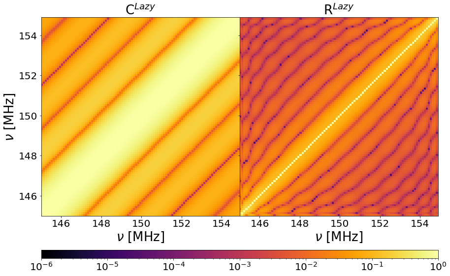
While $\boldsymbol{\mathsf{C}^{\daleth}}$ is Toeplitz, the actual weighting that we apply to visibility data, $\boldsymbol{\mathsf{R}^{\daleth}}$ is not (Fig. 1).

The Sinc foreground component to the covariance in equation (3.2) is diagonalized by a heavily studied set of orthonormal vectors known as discrete prolate spheroidal sequences (Slepian 1978, DPSSs,).

Letting $\mathcal{W}=\tau_{w}\Delta\nu$, Slepian 1978 define a DPSS $\boldsymbol{u^{(\alpha)}}(N_{\text{d}},\mathcal{W})$ to be one of the countable orthonormal set of vectors solving the eigenvalue problem

where

Since $\boldsymbol{\mathsf{L}}=2\mathcal{W}\boldsymbol{\mathsf{C}^{\daleth}}_{\text{FG}}$, the DPSSs also diagonalize $\boldsymbol{\mathsf{C}^{\daleth}}_{\text{FG}}$. Because $\boldsymbol{\mathsf{C}^{\daleth}}$ is the sum of $\boldsymbol{\mathsf{C}^{\daleth}}_{\text{FG}}$ and an identity term, DPSSs are also the eigenvectors of $\boldsymbol{\mathsf{C}^{\daleth}}$ as we show numerically in Fig. 2. Let $\left\{h_{n}\right\}_{N_{\text{d}}}$ be the set of all complex sequences of length $N_{\text{d}}$. Slepian 1978 show that $\boldsymbol{u^{(0)}}(N_{\text{d}},\mathcal{W})$ the DPSS with the largest eigenvalue $\lambda_{0}$ is the unit-norm $N_{\text{d}}$ sequence that maximizes the quantity

where $H(f)$ is the DFT of $h_{n}$ centered at $n=(N_{\text{d}}-1)/2$.

They also show that $\boldsymbol{u^{(1)}}(N_{\text{d}},\mathcal{W})$ is the vector that simultaneously maximizes $\mu$, has unity norm, and is orthogonal to $\boldsymbol{u^{(0)}}(N_{\text{d}},\mathcal{W})$. More generally, $\boldsymbol{u^{(\alpha)}}\left(N_{\text{d}},\mathcal{W}\right)$ is the vector that simultaneously maximizes $\mu$, has unity norm, and is orthogonal to the vectors in the set $\left\{\boldsymbol{u^{(\alpha^{\prime})}}\left(N_{\text{d}},\mathcal{W}\right):\alpha^{\prime}<\alpha\right\}$.

It follows that DPSSs have the ideal property of maximally concentrating power into a rectangular region of Fourier space with half-bandwidth $\tau_{w}$. The DPSS with the largest eigenvalue is the unity norm $N_{\text{d}}$ length sequence that concentrates maximal power (as quantified by $\mu$) within $\tau_{w}$. The DPSS with the second largest eigenvalue is the unity norm $N_{\text{d}}$-length sequence that maximally concentrates power within $\tau_{w}$ and is orthogonal to the DPSS with the largest eigenvalue. Ordering DPSSs by their eigenvalues (largest to smallest), the $\alpha^{th}$ DPSS for $N_{\text{d}}$ and $\tau_{w}$ is the length $N_{\text{d}}$ unity-norm sequence that maximally concentrates power within $\tau_{w}$ and is orthogonal to all $\alpha^{\prime}<\alpha$ DPSSs. Thus, our foreground covariance is diagonalized by the basis that most efficiently concentrates power within $\tau<\tau_{w}$. In the absence of channel flags, DPSS vectors are the eigenbasis of $\boldsymbol{\mathsf{C}^{\daleth}}$. As we discussed in § 3.1 though this covariance may not include the detailed information on the true values of $\lambda_{f}$ for each foreground mode on a particular baseline, as long as $\epsilon^{-1}$ is large enough, it will remove the foregrounds to a small enough level that we can measure the 21 cm signal in the presence of flagging side-lobes.

Slepian 1978 also show that the first $\approx 2N_{\text{d}}\mathcal{W}$ eigenvalues of $\boldsymbol{\mathsf{L}}$, $\lambda_{\alpha}(N_{\text{d}},\mathcal{W})$, are close to unity after which they rapidly drop to zero. When $N_{\text{d}}$ is small, the number of non-zero eigenvalues tends to exceed this number but it becomes increasingly accurate as $N_{\text{d}}$ increases. Fitting and characterizing foregrounds with DPSS vectors therefor requires $\approx 2B\tau_{w}$ components.

Under the realistic circumstance that there is missing data (e.g. RFI gaps), the eigenvectors are not equal to DPSSs. In Fig. 2, we compare the zeroth, second, and fourth numerically determined eigenvectors (ordered by decreasing eigenvalue) of $\boldsymbol{\mathsf{C}^{\daleth}}$ in Fig. 1 to DPSSs with length $N_{\text{d}}$, frequency bandwidth $B=10$ MHz, and delay-space width of $\tau_{w}=150$ ns. To within numerical precision, the DPSSs are identical to numerically computed eigenvectors of $\boldsymbol{\mathsf{C}^{\daleth}}$. We flag ten random channels in $\boldsymbol{\mathsf{C}^{\daleth}}$ by setting the corresponding rows and columns to zero and show the resulting eigenvectors with the zeroth, second, and fourth largest eigenvalues. The eigenvectors of $\boldsymbol{\mathsf{C}^{\daleth}}$ with flagged channels are not merely DPSSs with flagged elements equal to zero. Hence, when we have missing data (RFI gaps), we must set the corresponding rows and columns of $\boldsymbol{\mathsf{C}^{\daleth}}$ to zero and set $\boldsymbol{\mathsf{R}^{\daleth}}$ equal to the psuedo-inverse of this flagged covariance.

As stated in § 3.1, the effective action of $\boldsymbol{\mathsf{R}^{\daleth}}$ is to transform our data into a basis close to DPSSs where $\boldsymbol{\mathsf{C}^{\daleth}}$ is diagonal, divide the data by the eigenvalues of $\boldsymbol{\mathsf{C}^{\daleth}}$ in the $\boldsymbol{\mathsf{C}^{\daleth}}$ eigenbasis, and then transform back. The degree to which foreground removal and signal preservation are successful depends on how well isolated foreground and signal components are in the $\boldsymbol{\mathsf{C}^{\daleth}}$ eigenbasis and whether we have included sufficient dynamic range in the $\epsilon^{-1}$ parameter of $\boldsymbol{\mathsf{R}^{\daleth}}$.

As a first test, we apply it to a realization of a simplistic model autocorrelation for an isotropic sky with temperature $T_{\text{sky}}=60\,\mathrm{K}\,(\lambda/1\,\text{m})^{2.55}$, a chromatic Airy beam from a 14 m-diameter aperture, a receiver temperature of 100 K, and 200, evenly-spaced frequency channels, of width $\Delta\nu=100$ kHz between 140 MHz and 160 MHz. To simulate RFI flags, we randomly set the power levels in 20 channels to zero. To simulate thermal noise, we assume an integration time of $t_{\text{int}}=100$ hr, similar to what is necessary for a robust 21 cm detection, and set the standard deviation of each channel equal to $A/\sqrt{\Delta\nu t_{\text{int}}}$ where $A$ is the auto-correlation amplitude (Thompson et al. 2017). In Fig. 3, we show the impact of applying $\left[\boldsymbol{\mathsf{C}^{\daleth}}\right]^{-1}$ to a single realization of the autocorrelation with $\epsilon=10^{-10}$ and $\tau_{w}=50$ ns. After applying our filter, the foregrounds are suppressed by six orders of magnitude and the remaining residual (orange line) is very close to the original noise (green line). Taking the difference between the injected noise and residuals (dotted grey) we see that in the frequency domain, the filter residuals agree with the injected noise at the $\approx 10\%$ level.

In the bottom panel of Fig. 3 we inspect our simulation in the delay domain. In the absence of flags, we can use a 7-term Blackman-Harris⁴⁴ 4 The 7-term Blackman-Harris (see, for example Solomon 1993) includes additional sinusoidal terms beyond the standard 4-term Blackman-Harris found in standard libraries such as scipy.signal (Virtanen et al. 2020). While the additional terms increase the width of the central lobe, they substantially lower sidelobes compared to the typical 4-term implementation. We use a 7-term Blackman-Harris taper for all analysis in this paper and refer to it hereon out as simply “Blackman-Harris”. taper-filtered Fourier transform to suppress the impact of a finite sampling bandwidth beyond $\approx 250$ ns (solid grey line). When we set channels containing RFI to zero, these sharp edges spread foregrounds across all DFT modes (black dashed line). We compare the Blackman-Harris Fourier transform of residuals after applying $\boldsymbol{\mathsf{R}^{\daleth}}$ and the injected noise in delay space. The majority of the $\approx 10\%$ disagreement observed in frequency space is contained within 250 ns of the edge of our filter (shaded grey region).

Beyond 250 ns the injected noise and $\boldsymbol{\mathsf{R}^{\daleth}}$ residuals agree at the $\approx 10\%$ level. At $\tau\gtrsim 250$ ns, the leaked foregrounds are subtracted to the level of $10^{-8}$, even with flagging. This is much better than what can be accomplished by an apodized DFT with no flagging. Since apodization functions go to zero at the band edges, they also attenuate the signal. While we applied an apodization before DFTing $\boldsymbol{\mathsf{R}^{\daleth}}{\bf x}$ to obtain a more direct comparison with with the unflagged model in which no foregrounds were filtered, we technically didn’t have. Thus, applying $\boldsymbol{\mathsf{R}^{\daleth}}$ allows one to circumvent the band-edge signal attenuation that comes with apodization.

In this simplified example, $\boldsymbol{\mathsf{R}^{\daleth}}$ is highly effective at suppressing foregrounds. However, our simulation made a number of unrealistic assumptions. We assumed an isotropic sky with identical spectral indices. In addition, we assumed that the only chromaticity in our antenna response was sourced by its airy function beam pattern. Ultimately, $\boldsymbol{\mathsf{R}^{\daleth}}$ and any other inverse covariance filter schemes will only be effective if the foregrounds as viewed by the instrument are spanned by the model covariance’s foreground eigenmodes and the model covariance has enough dynamic range to suppress the foreground modes in the data to a level where their flagging side-lobes do not mask the 21 cm signal power-spectrum. For $\boldsymbol{\mathsf{R}^{\daleth}}$, this means that it will prevent foreground bleed by the DFT and missing data as long as $\epsilon$ is large enough and $\tau_{w}$ extends beyond the delays where the foregrounds convolved with the instrument exceed the 21 cm signal level. From a practical standpoint, this means that $\boldsymbol{\mathsf{R}^{\daleth}}$ cannot help us detect 21 cm fluctuations if interal and external antenna reflections as observed for example by Beardsley et al. 2016; Ewall-Wice et al. 2016a; Kern et al. 2019 extend into the delays where interferometers derive most of their sensitivity. On the other hand, if the signal chain chromaticity is contained within some upper $\tau_{w}$; a design requirement for the Hydrogen Epoch of Reionization Array (HERA) (DeBoer et al. 2017), then all an analyist needs to do in order to filter foregrounds from their data is to choose a large $\epsilon^{-1}$ and set an appropriate $\tau_{w}$ in $\boldsymbol{\mathsf{R}^{\daleth}}$ that extends to the horizon delay $\tau_{H}$ plus the intrinsic chromaticity of the antenna. Considering HERA as an example; the HERA antenna’s chromaticity leaks power above $\approx-50$ dB at $250$ ns (Ewall-Wice et al. 2016c; Thyagarajan et al. 2016; Patra et al. 2018). For HERA, we therefor recommend a $\tau_{w}$ equal to the wedge plus roughly $250$ ns.

To be an effective foreground filter, $\boldsymbol{\mathsf{R}^{\daleth}}$ should attenuate foregrounds while leaving as much of the 21 cm signal as untouched as possible. If 21 cm is also attenuated and we do not account for this attenuation in the normalization step we can end up with an unaccounted bias in our measurement: signal loss. Signal loss is not necessarily a bad thing and is in fact desirable if it suppresses foregrounds on otherwise contaminated 21 cm modes (we would not want our normalization to restore this). In paper II, we will explore when and how good signal loss occurs. In this paper, we focus on the attenuation properties of our simple filter DAYENU with the conservative assumption that we use $\boldsymbol{\mathsf{M}_{\text{ID}}}$ so no correction is made at the normalization step. Under these conditions we treat signal attenuation as significant if its power-spectrum signature exceeds sample variance errors which dominate the most sensitive regions of k-space in upcoming experiments. Lanman & Pober 2019 find that sample variance errors for per-baseline power-spectra are on the order of $20\%$ which places a 10% constraint on attenuation in the visibility domain. Spherically averaged power-spectra are expected to be far more sensitive, with $\sim 2\%$ sample-variance errors. This places a constraint of 1% on visibility attenuation.

We investigate the degree that DAYENU can suppress modes with different $\tau$ by studying the amplitudes of ${\bf z}^{\tau}=\boldsymbol{\mathsf{R}^{\daleth}}{\bf x}^{\tau}$ where ${\bf x}^{\tau}$ is a complex sinusoid with delay $\tau$ and amplitude equal to unity sampled every $100$ kHz. In Fig. 4, we plot the RMS of ${\bf z}^{\tau}$, $\sqrt{N_{\text{d}}^{-1}\sum_{m}|z_{m}^{\tau}|^{2}}$ vs. $\tau$ for two bandwidths; $10$ MHz and $100$ MHz, $\epsilon=10^{-9}$, and two filter widths; $\tau_{w}=150$ ns and $\tau_{w}=500$ ns.

Within the attenuation region, we see that input tones are suppressed by a factor of $10^{-7}$ to $10^{-6}$, depending on the bandwidth with larger bandwidths achieving more effective suppression. When 10 MHz of bandwidth is used, $\gtrsim 10\%$ signal attenuation occurs within roughly $300$ ns of the filter edge. Performance improves dramatically if a filtering bandwidth of 100 MHz is used instead. For 100 MHz filtering, $\lesssim 10$% attenuation occurs beyond $50$ ns of the filter edge and $\lesssim 1$% attenuation is reached by 300 ns beyond the filter edge. Thus, if we conservatively choose to normalize with $\boldsymbol{\mathsf{M}_{\text{ID}}}$ then attenuation beyond $300$ ns will be smaller then the expected sample variance errors in upcoming experiments. $\boldsymbol{\mathsf{M}_{\text{ID}}}$ is a conservative choice however and we can do better if we choose normalizations that undo these attenuations which we explore in paper II.

We also inspect how the amplitude of ${\bf z}^{\tau}$ depends on $\epsilon$ in Fig. 5. We note that the overall level of suppression is consistent (within a few dB) whether we filter across 100 MHz or 10 MHz. We compute the average level of suppression of tones over a range of $\tau_{w}$ and bandwidths as a function of $\epsilon$ in Fig. 6. For a fixed $\epsilon$, the amplitudes of residuals within the filtering region agree within $0.25$ dex over a wide range of $\tau_{w}$ and bandwidths. The RMS suppression of Fourier tones within the filtering region follows a power law which we fit to be RMS$\approx 0.1\epsilon^{0.5}$. It follows that to suppression 21 cm foregrounds which are $\approx 10^{4}$ times larger then cosmological fluctuations, we should apply filters with $\epsilon\lesssim 10^{-8}$. Since the foregrounds in the EoR window will be suppressed by flagging side-lobes, it is possible that one could get away with $\epsilon$ one-to-two orders of magnitude larger depending on the severity of flagging.

To derive $\boldsymbol{\mathsf{C}^{\daleth}}$ (equation 3.2), we wrote down discrete elements of our frequency covariance matrix by taking the continuous Fourier transform of a covariance that was diagonal in continuous delay space. On the other hand, many power spectrum estimators (e.g., Parsons et al. 2012b; Dillon et al. 2013; Trott et al. 2016; Barry et al. 2019) estimate band-powers in DFT space. This difference in approach immediately raises the question, why not derive $\boldsymbol{\mathsf{R}}$ from a covariance matrix that is diagonal in DFT space rather than the continuous space that we chose? After all, if we could just write down $\boldsymbol{\mathsf{R}}$ as diagonal in DFT space, could we just divide the DFT of our data-set by the diagonal DFT of $\boldsymbol{\mathsf{R}}$,$\boldsymbol{\widetilde{\mathsf{R}}}$, and save computational steps? The short answer is that an $\boldsymbol{\mathsf{R}}$ that is diagonal in DFT space only includes information on foreground modes with delays equal to $m/B,m\in\{-N_{\text{d}}/2,\dots N_{\text{d}}/2-1\}$ and as a result is incapable of properly suppressing foregrounds at intermediate delays. In order to see this effect, we write $\boldsymbol{\mathsf{C}}^{\text{DFT}}$ as the discrete Fourier transform of a covariance that is diagonal in DFT space,

We then transform $\boldsymbol{\widetilde{\mathsf{C}}}^{\text{DFT}}$ into discrete frequency space by performing a 2D DFT.

where we used the Poisson summation formula (e.g., Epstein 2007) to go from the second and third lines in equation 3.6. We see that the foreground component of $\boldsymbol{\mathsf{C}^{\text{DFT}}}$ is essentially an infinite sum of copies of the foreground component of $\boldsymbol{\mathsf{C}^{\daleth}}$ translated along the diagonal by integer multiples of $B$. This can also be seen by visual inspection in Fig. 7 where we plot $\boldsymbol{\mathsf{C}^{\daleth}}$ next to $\boldsymbol{\mathsf{C}^{\text{DFT}}}$. The wrap-around arises from the fact that our covariance elements are exclusively comprised of tones that are periodic over the interval $B$.

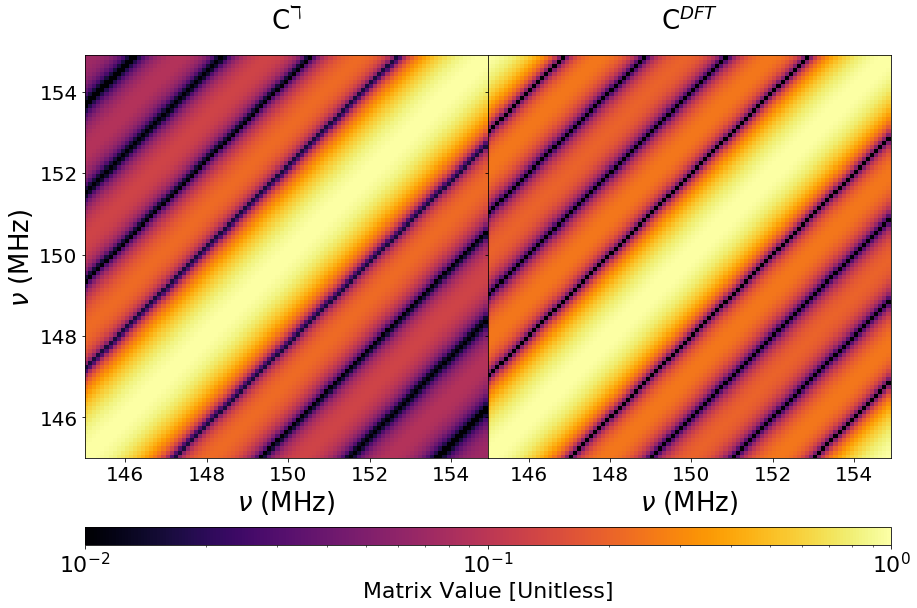
By definition, $\boldsymbol{\mathsf{C}^{\text{DFT}}}$ is diagonalized by the DFT. Thus, when we weight by its inverse, it will only down-weight modes with $\tau=mB^{-1}\leq\tau_{w}$; harmonic or on-grid DFT tones. Visibilities include a continuum of delays and only a fraction of their power is accounted for by harmonic tones within the wedge. Thus, $\boldsymbol{\mathsf{R}}^{\text{DFT}}\equiv\left[\boldsymbol{\mathsf{C}^{\text{DFT}}}\right]^{-1}$ is incapable of removing the bulk of foreground power, especially power in the sinc-sidelobes of the aharmonic tones. These side-lobes remain at high delays and prohibit a 21 cm measurement.

Figure 8 illustrates the limitations of $\boldsymbol{\mathsf{C}}^{\text{DFT}}$, where we show the same quantities as in Fig. 4 but now include the performance of $\boldsymbol{\mathsf{R}}^{\text{DFT}}$. We study the impact of progressively adding in-between-modes back into $\boldsymbol{\mathsf{C}}^{\text{DFT}}$ by increasing the wrap-around interval in equation 3.6. For example, increasing the wrap-around from $B$ to $2B$, adds additional modes that are periodic over a bandwidth of $2B$ but are not periodic over $B$. The orange lines in Fig. 8 show the residual amplitudes leftover after applying $\boldsymbol{\mathsf{R}}^{\text{DFT}}$ to complex sinusoides with various delays, $\tau$. Unlike $\boldsymbol{\mathsf{R}^{\daleth}}$, gaps are present, $\boldsymbol{\mathsf{R}}^{\text{DFT}}$’s filter coverage and truely effective filtering only occurs at $\tau=m/B,m\in\mathbb{Z}$. Between $B^{-1}$ harmonics, filtering only decreases the foreground amplitude by a factor of $\sim 10^{-1}$.

As we increase period of the wrap-around in equation 3.6, the harmonic filter tones move closer together and eventually merge. Because larger bandwidths have greater Fourier resolution, increasing the DFT wrap-around to 2B over 100 MHz actually attains similar performance for the completely continuous case though DAYENU still subtracts foregrounds to roughly $\approx 10^{-2}\times$ the level of DFT modes at the filter edge. This indicates that if we did want to use DFT modes to model our foregrounds and subract them, we need on the order of $\gtrsim 2\times$ as many modes. Since $\boldsymbol{\mathsf{C}^{\text{DFT}}}$ converges to DAYENU as the wrap interval approaches $\gtrsim 2B$, roughly $\gtrsim 4\tau_{w}B$ DFT modes are necessary to model foregrounds at a level similar to $\approx 2\tau_{w}B$ DPSS vectors. As we mentioned in § 3.3, for large $N_{\text{d}}$, the number of DPSS modes with non-zero eigenvalues in $\boldsymbol{\mathsf{C}^{\daleth}}$ is approximately $2B\tau_{w}$.

If the DPSS modes are precomputed and the number of DPSS modes being fit is much less then the number of frequency channels, then finding the fit coefficients for a single flagging pattern and set of fitted modes is dominated by calculating $\boldsymbol{\mathsf{A}}^{\dagger}\boldsymbol{\mathsf{w}}\boldsymbol{\mathsf{A}}$ where $\boldsymbol{\mathsf{A}}$ is the $N_{\text{d}}\times N_{\text{mode}}$ design matrix where each row is one of the $N_{\text{mode}}$ DPSS vectors that we are fitting. This matrix multiplication requires $\sim\mathcal{O}(N_{\text{d}}N_{\text{mode}}^{2})$ operations. Since typically twice as many DFT modes are required then DPSS modes, DPSS fitting with pre-computed modes reduces computational operations by a factor of four.

In summary, filtering with a covariance that is diagonal in the discrete Fourier basis will perform very poorly in foreground subtraction because it only contains the subset of foreground modes that are harmonics of $B^{-1}$. In defining $\boldsymbol{\mathsf{C}^{\daleth}}$, we instead allow foregrounds to include any continuous delay within the wedge and use numerical matrix inversion determine and downweight a discrete set of principal components.

It is clear from Fig. 4 that the larger the bandwidth we filter over, the smaller the unwanted signal attenuation outside of $\tau_{w}$. This motivates the use of $\sim 100$ MHz bandwidths for filtering. The power spectrum is usually approximated over bandwidths of $\lesssim 10$ MHz in order to ensure roughly stationary statistics for the evolving 21 cm signal.

These two ends can simultaneously be achieved by applying $\boldsymbol{\mathsf{R}^{\daleth}}$ over a $\approx 100$ MHz band, truncating, and then estimating the power spectrum from a DFT over a smaller sub-band. Under this scheme, $\boldsymbol{\mathsf{R}^{\daleth}}$ is a non-square $N_{\text{d}}\times N_{\text{d}}^{\text{F}}$ matrix, where $N_{\text{d}}^{\text{F}}$ is the number of channels to be filtered over and $N_{\text{d}}^{\text{F}}\geq N_{\text{d}}$. To obtain a truncated $\boldsymbol{\mathsf{R}^{\daleth}}$, all we have to do is zero out the rows of $\boldsymbol{\mathsf{R}^{\daleth}}$ corresponding to channels that we do not want to include in the application of $\boldsymbol{\mathsf{Q}_{\alpha}}$.

Fig. 9 examines signal attenuation as a function $\tau$ over ten different $10$ MHz sub-bands where truncation to $10$ MHz is performed after the application of $\boldsymbol{\mathsf{R}^{\daleth}}$. In each sub-band, signal attenuation is dramatically reduced compared to filtering over the 10 MHz band alone. With the exception of the edge bands (100-110 MHz and 190-200 MHz), $\lesssim 1$ % signal attenuation is achieved by 250 ns beyond the filter edge. In the outer 10 MHz bands, 10% loss is still achieved by 150-200 ns off the filter edge. In light of these results, we recommend sub-band power-spectrum estimates be obtained from data on which DAYENU is applied over as wide a band as possible and then truncated.

In real life, some fraction of interferometric channels are contaminated by RFI and must be discarded. Thus, it is necessary for DAYENU to work robustly on data that is not evenly sampled. We investigate the impact of RFI flagging by inspecting RMS residuals from applying the psuedo-inverse of $\boldsymbol{\mathsf{C}^{\daleth}}$ where rows and columns corresponding to flagged channels are set to zero. We explore two different scenarios over 100 MHz of bandwidth. One in which twenty percent of channels are flagged randomly and one in which 200 kHz flags are applied every 1.28 MHz; similar to what must be performed on the MWA (Dillon et al. 2015; Ewall-Wice et al. 2016b; Beardsley et al. 2016; Barry et al. 2019) (Fig. 10). Since the MWA records $\approx 30$ MHz simultaneously, we also show the RMS residual of $\boldsymbol{\mathsf{R}^{\daleth}}$ with 200 kHz flags every 1.28 MHz over 30 MHz.

WIth 200 100 kHz channels flagged randomly over 100 MHz, we find that attenuation beyond the filter width increases by approximately 1% out to large delays. The presence of periodic flags results in the flagging attenuation being concentrated in a concentrated region centered $\approx 781$ ns, the delay of the 1.28 MHz flag periodicity. Outside of this region, the attenuation is negligible but within this region it exceeds 2%, in excess of the average 1% induced by randomized flagging.

By subtracting foregrounds with a matrix multiplication, DAYENU accomplishes one of the primary objectives of the iterative CLEAN filter (Parsons et al. 2012b). ${\bf z}=\boldsymbol{\mathsf{R}^{\daleth}}{\bf x}$ is equivalent to the residual after CLEAN is applied. The second goal of CLEAN is to smoothly interpolate (restore) the subtracted foregrounds by adding back their CLEAN components; interpolating the foregrounds over flagged channel gaps with DFT modes. We can isolate the foregrounds subtracted by $\boldsymbol{\mathsf{R}^{\daleth}}$ with the matrix operation $(\boldsymbol{\mathsf{I}}-\boldsymbol{\mathsf{R}^{\daleth}})$ and fit them to $N_{\text{DPSS}}$ DPSS modes. DPSS vectors are eigenvectors of the foreground component of $\boldsymbol{\mathsf{C}^{\daleth}}$ so we can approximate our foregrounds with the DPSS vectors with eigenvalues above some small number relative to the largest eigenvalues. We choose a cutoff of $10^{-12}$ the largest eigenvalue which ensures that foreground modes are subtracted to a level of $\lesssim 10^{-6}$.

Fitting and interpolating with our $N_{\text{DPSS}}$ modes can be achieved applying the linear least squares solution matrix to $(\boldsymbol{\mathsf{I}}-\boldsymbol{\mathsf{R}^{\daleth}})$.

where $\boldsymbol{\mathsf{A}}$ is an $N_{\text{d}}\times N_{\text{DPSS}}$ matrix

where $u_{m}^{(\alpha)}(N_{\text{d}},\tau_{w})$ is the $m^{th}$ element of the $\alpha^{th}$ DPSS vector of length $N_{\text{d}}$ that diagnalizes the $N_{\text{d}}\times N_{\text{d}}$ matrix $\mathsf{S}_{mn}(N_{\text{d}},\tau_{w})=(2\tau_{w}\Delta\nu)\text{Sinc}\left[2\pi\tau_{w}(\nu_{m}-\nu_{n})\right]$ and $\boldsymbol{\mathsf{w}}$ is a diagonal matrix set to unity at unflagged channels and zero at flagged channels. Applying $\boldsymbol{\mathcal{A}}$ to $(\boldsymbol{\mathsf{I}}-\boldsymbol{\mathsf{R}^{\daleth}})$ provides us with DPSS interpolated CLEAN components. Adding these CLEAN components to the residual gives us a linear REST (restoration) matrix which both filters the data and interpolates the subtracted foregrounds.

We can understand the first term of equation 34 as follows. First $(\boldsymbol{\mathsf{I}}-\boldsymbol{\mathsf{R}^{\daleth}})$ is applied which effectively filters out all small-scale structure dominated by the 21 cm signal and contains RFI flagging gaps. Next, $\boldsymbol{\mathsf{A}}^{T}\boldsymbol{\mathsf{w}}$ transforms the flagged data into the DPSS basis. Mode-mixing between the DPSS coefficients, due to flagged channels, is undone by applying $\left[\boldsymbol{\mathsf{A}}^{T}\boldsymbol{\mathsf{w}}\boldsymbol{\mathsf{A}}\right]^{-1}$ and a final application of $\boldsymbol{\mathsf{A}}$ transforms back into frequency space. Thus, the total action of the first term is the interpolation over flagged channels with fitted smooth DPSS modes. The second term of equation 34 isolates the fine-frequency components of the signal including noise and the 21 cm signal itself.

In § 4, we will demonstrate the performance of DAYENUREST on realistic foreground and signal simulations.

In this section, we use simulated HERA visibilities (Kern et al. 2019, Appendix A,) to validate filtering with $\boldsymbol{\mathsf{R}^{\daleth}}$ along with the overall impact of this filtering on power-spectrum statistics. We construct our simulations using the healvis software (Lanman & Kern 2019), which integrates the visibility equation using a HEALpix representation of the sky (Górski et al. 2005). The simulations use the Global Sky Model (de Oliveira-Costa et al. 2008, GSM;) for the foreground model, and a flat-spectrum, uncorrelated random Gaussian field as the EoR model with a variance of 25 mK².

They also use a simplified model of the HERA primary beam in instrumental XX and YY polarization, assuming minimal frequency structure in the sidelobes of the beam. Specifically, the beam is low-pass filtered across frequency at every HEALpix pixel to reject structures for $|\tau|>250$ ns. For this work this is likely an inconsequential feature of the simulations, as it sets at which delay the foreground power dips below the EoR signal, which is not something that our analysis is sensitive to (Fagnoni et al. 2019). The simulations span eight hours of local sidereal time (LST) and have a frequency coverage from 120 – 180 MHz in 256 channels leading to a 235 kHz channelization. We refer the reader to (Lanman et al. 2019) for more details on the healvis package and (Kern et al. 2019) for further information on the simulated data products. Radio frequency interference plays a major role in setting the efficacy of these techniques. In this section, we use flagging masks representative of the RFI environment for HERA’s first observing season (Kerrigan et al. 2019; Kern et al. 2020).

Aside from being used as a filtering matrix in the final calculation of $\hat{p}_{\alpha}$, DAYENU can readily be employed in sandbox-type data analyses assessing the level of spectral structures in individual visibilities, data-cubes, and other products. In this section, we compare its efficacy to CLEAN filtering which is often used to a similar end. To do so, we inspect the performance of the direct application of DAYENU and DAYENUREST to our simulated visibilities, and compare our results to CLEAN. In the literature (e.g. (Kern et al. 2019)), CLEANing is performed on the visibility after zero-padding by $N_{\text{d}}$ channels on either side (For these simulations $N_{\text{d}}=256$) and taper-filtering with a Tukey window with $\alpha=0.15$. Zero-padding is performed to give CLEAN a larger number of Fourier modes to work with; allowing it to fit the same aharmonic delays that are absent from an $N_{\text{d}}$ DFT. We perform CLEANing over $\pm 150$ ns in delay-space. Each iteration of CLEAN finds the peak power of the data in delay-space and subtracts the peak power times $0.1$ (gain) times a flagging kernel centered at the peak delay until the RMS residual changes with each iteration by less than some fraction of the RMS of the original visibilities. The tolerance parameter can be set as low as we want to obtain some arbitrary degree of foreground subtraction. In practice, the choice of tolerance depends on the constraints of computational resources. We adopt $10^{-9}$ that is currently being used in the HERA analysis pipeline. In addition, for $N_{\text{d}}=256$, CLEANing a single baseline on a single time to $10^{-9}$ tolerance has a similar runtime (within an order of magnitude) of computing the psuedoinverse of $\boldsymbol{\mathsf{C}^{\daleth}}$ to obtain $\boldsymbol{\mathsf{R}^{\daleth}}$.

For ${\tt DAYENUREST}$, we limit the set of DPSS vectors to those with eigenvalues of $\boldsymbol{\mathsf{L}}$ greater then $10^{-12}$. As we stated in § 3.3, the maximum eigenvalue of $\boldsymbol{\mathsf{L}}$ is close to unity. We compare the sum of clean residuals and clean components, which interpolate over flagged channel gaps (Center Fig. 11), to DAYENURESTd simulations (Right Fig. 11). At large scales, our linear cleaning and interpolation technique performs just as well as CLEAN in reproducing macroscopic foreground features. In order to understand the low-level disagreements between the two, we inspect their residuals.

We compare the residuals from CLEAN and DAYENUREST (Fig. 12). For CLEAN, we refer to residuals as what is left in the data after iteratively subtracting all CLEAN-components and for DAYENU and DAYENUREST, as in the previous sections, residuals refer to the data after applying $\boldsymbol{\mathsf{R}^{\daleth}}$. Note that the residuals for DAYENU and DAYENUREST are identical by the definition of DAYENUREST (eq. 34). In Fig. 12, DAYENU and DAYENUREST subtract the foregrounds to below the 21 cm level (right panel) while CLEAN leaves significant residuals (center right panel). To understand the impact of flagging, we also inspect the residuals of CLEAN with no flagging (center left panel). The CLEAN residuals are nearly identical whether or not flagging is present. It follows that flagging alone does not impact the absolute level of residuals left after CLEANing. If these residuals instrinsically stay within the wedge, they will not have an impact on our ability to detect 21 cm outside of the wedge. However, the presence of flagged channels will cause the residuals to enter the EoR window at a level that depends on the flagging.

In Fig. 13, we compare the Blackman-Harris taper-filtered delay-transform of DAYENUREST and CLEAN filtered data with and without flagging across three different bands. For DAYENUREST filtered data refers to the data after the application of $\boldsymbol{\mathsf{R}^{\text{REST}}}$. For CLEAN filtered refers to CLEAN residuals plus the interpolating CLEAN components. Our three bands are as follows. First, the entire 120-180 MHz band. Second, a 120-138 MHz band below ORBCOMM which is heavily flagged, and thirdly $141-180$ MHz above ORBCOMM with roughly twice the bandwidth as below. With no RFI flagging, CLEAN and DAYENUREST perform similarly well as can be seen by comparing the red-solid and grey-solid lines in Fig. 13. Unfortunately, the presence of RFI flags causes significant bleed of the CLEAN filtered data outside of the wedge and is especially bad when the DFT band includes ORBCOMM at $137$ MHz. We also plot the residuals of CLEAN and DAYENUREST as dashed lines. The maximum low-delay level of CLEAN residuals is practically the same with and without flags. The presence of flags causes these residuals to bleed to high delays at levels much larger then 21 cm. Since the level of these bleeding residuals agrees with the level of the total filtered data, we conclude that the structures in CLEAN residuals introduced by flagging are to blame for high-delay contamination in the CLEAN filtered visibilities. Even without ORBCOMM, leakage of CLEAN residuals exceeds our injected 21 cm signal by a factor of a few. DAYENUREST (red-solid line) successfully removes foregrounds below the level of the 21 cm signal (black dotted line) in all cases. The relatively narrow bandwidth below ORBCOMM, presents a potential challenge since the central foregound lobe extends to $k_{\parallel}\approx 0.2h$Mpc^-1. Losing $k_{\parallel}\lesssim 0.2h$ Mpc^-1 to foregrounds has a significant impact on science returns (Pober et al. 2014; Ewall-Wice et al. 2016a; Ewall-Wice et al. 2016c). In § 4.3, we investigate whether the central foreground lobe is actually a fundamental limitation.

Over 256 channels, CLEAN’s runtime per integration is also significantly larger than DAYENUREST’s. With our adopted parameters, on a laptop with a 2.4 GHz i5 processor, computing $\boldsymbol{\mathsf{R}^{\daleth}}$ for each unique flagging pattern and set of filter-widths, centers, and suppression factors takes roughly 0.24 seconds while filtering a baseline at a single time with a cached filter matrix takes approximately $0.003$ seconds. In comparison, the time for CLEAN to run on each baseline-time is $0.8$ seconds and there is no possibility of speeding things up through caching.

kBefore we move on to power-spectra, it is worth noting that although we have focused filtering visibilities, $\boldsymbol{\mathsf{R}^{\daleth}}$ can just as easily be used to foreground-filter gridded visibilites by applying $\boldsymbol{\mathsf{R}^{\daleth}}$ along the frequency axis of each $uv$ cell. In this situation, one would set $\tau_{w}$ to include not only the intrinsic chromaticity of the antenna and the wedge in the $uv$ cell but also to include any additional spectral structure that might be introduced by gridding. We leave the question of how much one would need to increase $\tau_{w}$ for different gridding strategies to future work.

We now explore the impact that various choices of $\boldsymbol{\mathsf{R}}$ have on the final power spectrum when when we use identity normalization $\boldsymbol{\mathsf{M}}\propto\boldsymbol{\mathsf{M}_{\text{ID}}}$. We calculate a normalized ${\bf\hat{p}}$ from 42 channels between 145 MHz and 155 MHz; corresponding to a redshift interval of $\Delta z\approx 0.5$ for the following choices of $\boldsymbol{\mathsf{R}}$.

• •

  Blackman-Harris: We use an apodization filter with the diagonal set equal to a 7-term Blackman-Harris taper function $\boldsymbol{\mathsf{R}}=\boldsymbol{\mathsf{R}}^{\text{BH}}$. To obtain a noise-equivalent bandwidth of 10 MHz, we extend the spectral window to 96 channels (22.5 MHz).

• •

  No Flags: A scenario for reference. The same as Simple Delay-Spectrum but with no RFI flagging. In this scenario, we also have $\boldsymbol{\mathsf{R}}=\boldsymbol{\mathsf{R}}^{\text{\bf BH}}$

• •

  DAYENU Narrowband: Apply $\boldsymbol{\mathsf{R}^{\daleth}}$ with $\epsilon=10^{-9}$ and $\tau_{w}=150$ ns across the same bandwidth as the Fourier Transform (42 channels – 10 MHz; $\boldsymbol{\mathsf{R}^{\daleth}}$). We do not use a taper in the Fourier transform. Thus $\boldsymbol{\mathsf{R}}=\boldsymbol{\mathsf{R}^{\daleth}}$.

• •

  DAYENU Restored: Perform linear inpainting of foregrounds using DAYENUREST with a 150 ns attenuation region and in-painting modes spaced by 44.44 ns ($\boldsymbol{\mathsf{R}^{\text{REST}}}$). An identical Blackman-Harris tapered Fourier transform as our Blackman-Harris scenario is used to estimate bandpowers from the filtered data. Thus $\boldsymbol{\mathsf{R}}=\boldsymbol{\mathsf{R}}^{\text{\bf BH}}\boldsymbol{\mathsf{R}}^{\text{\bf REST}}$.

• •

  DAYENU Extended Filter: We perform filtering across the entire 60 MHz band with $\boldsymbol{\mathsf{R}^{\daleth}}$ before truncating and performing a DFT across the central 10 MHz. $\boldsymbol{\mathsf{R}}=\boldsymbol{\mathsf{R}^{\daleth}}$.

In all cases, we use $\boldsymbol{\mathsf{Q}_{\alpha}}=\boldsymbol{\mathsf{Q}_{\alpha}}^{\text{\bf DFT}}$. In order to convert our power spectra from visibility to cosmological units, we multiply $\boldsymbol{\mathsf{M}_{\text{ID}}}$ by a constant

where

, $\Omega_{pp}$ is the solid angle integral of the primary beam squared and averaged over our band of interest, $Y=dr_{\parallel}/d\nu$, $X=dr_{\perp}/d\theta$, $\lambda$ is the average observation wavelength, and $k_{B}$ is the Boltzmann constant. We refer the reader to Morales & Hewitt 2004; Parsons et al. 2012a; Parsons et al. 2014 for more the full expressions of these constants and their derivations. We estimate power spectra from eight hours of LST by computing an independent $\boldsymbol{\hat{p}}$ every 30.6 seconds and incoherently averaging. Our bandpower estimates appear in Fig. 14 along estimates of vertical and horizontal 68% confidence errorbars. We derive these confidence intervals from estimates of the bandpower covariances $\boldsymbol{\hat{\Sigma}}$ and window-functions $\boldsymbol{\hat{\mathsf{W}}}$. Before we discuss the results in this plot we first describe our calculations $\boldsymbol{\hat{\Sigma}}$ (§ 4.3.1) and $\boldsymbol{\hat{\mathsf{W}}}$ (§ 4.3.2).

References

- Ali et al. (2015) Ali Z. S., et al., 2015, ApJ, 809, 61
- Anderson et al. (2018) Anderson C. J., et al., 2018, MNRAS, 476, 3382
- Bandura et al. (2014) Bandura K., et al., 2014, Canadian Hydrogen Intensity Mapping Experiment (CHIME) pathfinder. p. 914522, doi:10.1117/12.2054950
- Barry et al. (2019) Barry N., Beardsley A. P., Byrne R., Hazelton B., Morales M. F., Pober J. C., Sullivan I., 2019, Publ. Astron. Soc. Australia, 36, e026
- Beardsley et al. (2016) Beardsley A. P., et al., 2016, ApJ, 833, 102
- Blake & Wall (2002) Blake C., Wall J., 2002, MNRAS, 337, 993
- Carroll et al. (2016) Carroll P. A., et al., 2016, MNRAS, 461, 4151
- Chang et al. (2010) Chang T.-C., Pen U.-L., Bandura K., Peterson J. B., 2010, Nature, 466, 463
- Chapman et al. (2012) Chapman E., et al., 2012, MNRAS, 423, 2518
- Chen (2015) Chen X., 2015, in IAU General Assembly. p. 2252187
- Cheng et al. (2018) Cheng C., et al., 2018, The Astrophysical Journal, 868, 26
- Datta et al. (2010) Datta A., Bowman J. D., Carilli C. L., 2010, ApJ, 724, 526
- DeBoer et al. (2017) DeBoer D. R., et al., 2017, PASP, 129, 045001
- Di Matteo et al. (2004) Di Matteo T., Ciardi B., Miniati F., 2004, MNRAS, 355, 1053
- Dillon et al. (2013) Dillon J. S., Liu A., Tegmark M., 2013, Phys. Rev. D, 87, 043005
- Dillon et al. (2015) Dillon J. S., et al., 2015, Phys. Rev. D, 91, 123011
- Eastwood et al. (2018) Eastwood M. W., et al., 2018, AJ, 156, 32
- Ellingson et al. (2009) Ellingson S. W., Clarke T. E., Cohen A., Craig J., Kassim N. E., Pihlstrom Y., Rickard L. J., Taylor G. B., 2009, IEEE Proceedings, 97, 1421
- Epstein (2007) Epstein C., 2007, Introduction to the Mathematics of Medical Imaging, 2 edn. Society for Industrial and Applied Mathematics, Philadelphia, PA (https://epubs.siam.org/doi/pdf/10.1137/9780898717792), doi:10.1137/9780898717792, https://epubs.siam.org/doi/abs/10.1137/9780898717792
- Ewall-Wice et al. (2016a) Ewall-Wice A., Hewitt J., Mesinger A., Dillon J. S., Liu A., Pober J., 2016a, MNRAS, 458, 2710
- Ewall-Wice et al. (2016b) Ewall-Wice A., et al., 2016b, MNRAS, 460, 4320
- Ewall-Wice et al. (2016c) Ewall-Wice A., et al., 2016c, ApJ, 831, 196
- Fagnoni et al. (2019) Fagnoni N., et al., 2019, arXiv e-prints, p. arXiv:1908.02383
- Górski et al. (2005) Górski K. M., Hivon E., Banday A. J., Wand elt B. D., Hansen F. K., Reinecke M., Bartelmann M., 2005, ApJ, 622, 759
- Hazelton et al. (2017) Hazelton B. J., Jacobs D. C., Pober J. C., Beardsley A. P., 2017, The Journal of Open Source Software, 2, 140
- Högbom (1974) Högbom J. A., 1974, A&AS, 15, 417
- Hunter (2007) Hunter J. D., 2007, Computing in Science & Engineering, 9, 90
- Jacobs et al. (2011) Jacobs D. C., et al., 2011, ApJ, 734, L34
- Jacobs et al. (2016) Jacobs D. C., et al., 2016, ApJ, 825, 114
- Jacobs et al. (2017) Jacobs D. C., et al., 2017, PASP, 129, 035002
- Kern et al. (2019) Kern N. S., Parsons A. R., Dillon J. S., Lanman A. E., Fagnoni N., de Lera Acedo E., 2019, arXiv e-prints, p. arXiv:1909.11732
- Kern et al. (2020) Kern N. S., et al., 2020, ApJ, 888, 70
- Kerrigan et al. (2019) Kerrigan J., et al., 2019, MNRAS, 488, 2605
- Kolopanis et al. (2019) Kolopanis M., et al., 2019, ApJ, 883, 133
- Lanman & Kern (2019) Lanman A. E., Kern N., 2019, healvis: Radio interferometric visibility simulator based on HEALpix maps (ascl:1907.002)
- Lanman & Pober (2019) Lanman A. E., Pober J. C., 2019, MNRAS, 487, 5840
- Lanman et al. (2019) Lanman A. E., Pober J. C., Kern N. S., de Lera Acedo E., DeBoer D. R., Fagnoni N., 2019, arXiv e-prints, p. arXiv:1910.10573
- Line et al. (2017) Line J. L. B., Webster R. L., Pindor B., Mitchell D. A., Trott C. M., 2017, Publ. Astron. Soc. Australia, 34, e003
- Liu & Shaw (2019) Liu A., Shaw J. R., 2019, arXiv e-prints, p. arXiv:1907.08211
- Liu & Tegmark (2011) Liu A., Tegmark M., 2011, Phys. Rev. D, 83, 103006
- Liu et al. (2014a) Liu A., Parsons A. R., Trott C. M., 2014a, Physical Review D, 90, 023018
- Liu et al. (2014b) Liu A., Parsons A. R., Trott C. M., 2014b, Phys. Rev. D, 90, 023019
- Lomb (1976) Lomb N. R., 1976, Ap&SS, 39, 447
- Masui et al. (2013) Masui K. W., et al., 2013, ApJ, 763, L20
- Mertens et al. (2020) Mertens F. G., et al., 2020, MNRAS, 493, 1662
- Morales & Hewitt (2004) Morales M. F., Hewitt J., 2004, ApJ, 615, 7
- Morales et al. (2012) Morales M. F., Hazelton B., Sullivan I., Beardsley A., 2012, ApJ, 752, 137
- Neben et al. (2015) Neben A. R., et al., 2015, Radio Science, 50, 614
- Neben et al. (2016) Neben A. R., et al., 2016, ApJ, 826, 199
- Newburgh et al. (2016) Newburgh L. B., et al., 2016, HIRAX: a probe of dark energy and radio transients. p. 99065X, doi:10.1117/12.2234286
- Parsons et al. (2012a) Parsons A., Pober J., McQuinn M., Jacobs D., Aguirre J., 2012a, ApJ, 753, 81
- Parsons et al. (2012b) Parsons A. R., Pober J. C., Aguirre J. E., Carilli C. L., Jacobs D. C., Moore D. F., 2012b, ApJ, 756, 165
- Parsons et al. (2014) Parsons A. R., et al., 2014, ApJ, 788, 106
- Patil et al. (2016) Patil A. H., et al., 2016, MNRAS, 463, 4317
- Patra et al. (2018) Patra N., et al., 2018, Experimental Astronomy, 45, 177
- Pober et al. (2012) Pober J. C., et al., 2012, AJ, 143, 53
- Pober et al. (2013) Pober J. C., et al., 2013, ApJ, 768, L36
- Pober et al. (2014) Pober J. C., et al., 2014, ApJ, 782, 66
- Scargle (1982) Scargle J. D., 1982, ApJ, 263, 835
- Shaw et al. (2014) Shaw J. R., Sigurdson K., Pen U.-L., Stebbins A., Sitwell M., 2014, ApJ, 781, 57
- Slepian (1978) Slepian D., 1978, AT T Technical Journal, 57, 1371
- Solomon (1993) Solomon O. M. J., 1993, Technical report, The use of DFT windows in signal-to-noise ratio and harmonic distortion computations
- Subrahmanya et al. (2017) Subrahmanya C. R., Manoharan P. K., Chengalur J. N., 2017, Journal of Astrophysics and Astronomy, 38, 10
- Switzer et al. (2013) Switzer E. R., et al., 2013, MNRAS, 434, L46
- Switzer et al. (2015) Switzer E. R., Chang T. C., Masui K. W., Pen U. L., Voytek T. C., 2015, ApJ, 815, 51
- Tegmark (1997) Tegmark M., 1997, Phys. Rev. D, 55, 5895
- Thompson et al. (2017) Thompson A. R., Moran J. M., Swenson George W. J., 2017, Interferometry and Synthesis in Radio Astronomy, 3rd Edition, doi:10.1007/978-3-319-44431-4.
- Thyagarajan et al. (2016) Thyagarajan N., Parsons A. R., DeBoer D. R., Bowman J. D., Ewall-Wice A. M., Neben A. R., Patra N., 2016, ApJ, 825, 9
- Tingay et al. (2013) Tingay S. J., et al., 2013, Publ. Astron. Soc. Australia, 30, e007
- Trott et al. (2016) Trott C. M., et al., 2016, ApJ, 818, 139
- Vedantham et al. (2012) Vedantham H., Udaya Shankar N., Subrahmanyan R., 2012, ApJ, 745, 176
- Virtanen et al. (2020) Virtanen P., et al., 2020, Nature Methods, 17, 261
- Zhang et al. (2018) Zhang Y. G., Liu A., Parsons A. R., 2018, ApJ, 852, 110
- Zheng et al. (2017) Zheng H., et al., 2017, MNRAS, 464, 3486
- de Oliveira-Costa et al. (2008) de Oliveira-Costa A., Tegmark M., Gaensler B. M., Jonas J., Landecker T. L., Reich P., 2008, MNRAS, 388, 247
- van Haarlem et al. (2013) van Haarlem M. P., et al., 2013, A&A, 556, A2
Acknowledgements
We thank Jacqueline Hewitt, Honggeun Kim, Kevin Bandura, Miguel Morales, Bobby Pascua, Bryna Hazelton, and Ue-Li Pen for helpful discussions. AEW and acknowledges support from the NASA Postdoctoral Program and the Berkeley Center of Cosmological Physics. JSD gratefully acknowledges the support of the NSF AAPF award #1701536. A portion of this work was carried out at the Jet Propulsion Laboratory, California Institute of Technology, under a contract with the National Aeronautics and Space Administration. AL acknowledges support from the New Frontiers in Research Fund Exploration grant program, a Natural Sciences and Engineering Research Council of Canada (NSERC) Discovery Grant and a Discovery Launch Supplement, the Sloan Research Fellowship, as well as the Canadian Institute for Advanced Research (CIFAR) Azrieli Global Scholars program. This material is based upon work supported by the National Science Foundation under grants #1636646 and #1836019 and institutional support from the HERA collaboration partners. This research is funded in part by the Gordon and Betty Moore Foundation. HERA is hosted by the South African Radio Astronomy Observatory, which is a facility of the National Research Foundation, an agency of the Department of Science and Innovation.
Appendix A The Dependence of CLEAN residual amplitudes on the tolerance parameter.
In our comparison, we assumed a fixed set of CLEAN parameters employed by the HERA pipeline (Kern et al. 2019) and the RFI environment of the Karoo radio observatory. The presence of flagging leaks residuals left over by CLEANing across all delays. Hampering a 21 cm detection. Lowering the residuals also lowers this leakage so in principal decreasing the tolerance should allow for sufficiently low residuals for a 21 cm detection. In this appendix, we examine the CLEAN performance as a function of flagging percentage and tolerance parameter. We run CLEAN for a single model baseline and time across all 256 channels with 256 channel zero-padding on either side and a Tukey taper. We iteratively increase the width of flagging on the ORBCOMM band; starting with no flags, then introducing two 235 kHz channels centered at 137 MHz. Next, we introduce four channels, eights channels, and sixteen channels. In the top-panel of Fig. 17, we compare residuals for different levels of flagging to the injected 21 cm signal. Even when two channels are flagged, significant deviations are introduced in CLEAN when the tolerance is set to (solid colored lines). On the other hand, DAYENUREST reproduces both the foregrounds and signal with no residual bias.
As we mentioned above, the biases from CLEAN arise from foreground residuals that have not been fully subtracted and still contain side-lobes from flagging. By decreasing the tol parameter in CLEAN, we can actually subtract deeper. Thus, in principal there should exist small enough values OF THE tolerance such that side-lobes are suppressed enough to recover 21 cm fluctuations without signifant foreground bias. We explore this possiblity by lowering the tolerance to (Fig. 17 bottom-panel). Given this lower value, residuals are not visibly present with two flagged channels but biases appear after channels (only 3.1% of the data) are flagged. Running CLEAN with tol= takes 22 seconds per baseline and time-sample on a 2.4 GHz i5 processor – times slower then the linear filter if is computed at every baseline time and times slower then the realistic scenario where all baseline-times can be filtered with cached matrices.
While decreasing the tolerance can lower foreground leakage, there are diminishing returns and even after a performance hit relative to DAYENU, we run into trouble with just of channels flagged.