Marshall-Olkin exponential shock model covering all range of dependenceJournal: Journal Name
Abstract
In this paper, we present a new Marshall-Olkin exponential shock model. The new construction method gives the proposed model further ability to allocate the common joint shock on each of the components, making it suitable for application in fields like reliability and credit risk. The given model has a singular part and supports both positive and negative dependence structure. Main dependence properties of the model is given and an analysis of stress-strength is presented. After a performance analysis on the estimator of parameters, a real data is studied. Finally, we give the multivariate version of the proposed model and its main properties.
Keywords:
Shock model , Marshall-Olkin model , Negative and positive dependence2010 MSC
60E05, 60E15, 62N05.1 Introduction
The univariate exponential distribution is known for its applications in different fields such as reliability, telecommunication, hydrology, medical sciences and environmental science (see Balakrishnan 2018). One of the main multivariate extensions of exponential distribution was given by Marshall and Olkin 1967. They constructed their model based on shock models. Let , , , then the Marshall-Olkin (MO) shock model is achieved by
| (1.1) |
They showed that their extension verifies the lack of memory property in the multivariate case. The MO exponential distribution has both singular and continuous parts in its density and covers positive dependence structure. The MO model has a broad application in reliability (see Cherubini et al. 2015), finance and actuarial science (see Elouerkhaoui 2017 and Lindskog and McNeil 2003). For instance, Lindskog and McNeil 2003 applied the MO model to credit risk. They stated the MO model allows the applicability of dependence among the shock arrival times while it preserves exponentially distributed observed lifetimes. Also, Cherubini and Mulinacci 2017 expressed that within the concept of credit risk and financial crisis, the MO model gives an important and flexible tool to study and represent systemic crises. First, they asserted that, the MO model uses the unobserved shocks which are subject to each individual or common among individuals. Second, the common shocks are used for simultaneous default of the elements in the cluster stated as individual subsets disclosed to the same common factor. Third, the MO model preserves the marginal exponential distribution used for observed default times.
Many bivariate and multivariate extensions of exponential distribution have been introduced and applied in reliability. Esary and Marshall 1974 characterized a multivariate exponential distribution and derived a positive dependence condition for multivariate distributions with exponential minimum. Raftery 1984 proposed a continuous multivariate exponential distribution which can model a full range of correlation and attain the Fréchet bounds in the bivariate case. Tawn 1990 introduced a multivariate exponential distribution that arises from limiting joint distribution of normalized component-wise maxima or minima. Lin et al. 1993 used a shared-load model of the multivariate exponential distribution to describe the characteristics of dependent redundancies. The multivariate exponential distributions with constant failure rates has been given by Basu and Sun 1997. The multivariate power exponential distribution was given by Gómez et al. 1998. Cui and Li 2007 propose an analytical method for reliability of coherent systems with dependent components based on MO model. Fan et al. 2009 proposed a multivariate exponential survival tree procedure that splits data using the score test statistic derived from a parametric exponential frailty model, which allows for fast evaluation of splits. Kundu and Gupta 2009 estimated the parameter of a new bivariate exponential distribution using EM-algorithm. Li and Pellerey 2011 gave a generalization of bivariate MO distributions, which the well-known MO model includes as special case. Kundu and Gupta 2013 did a Bayesian estimation for the MO bivariate Weibull distribution. Bayramoglu and Ozkut 2014 used a MO model system by taking into account the system structure. Kundu et al. 2014 introduced a multivariate proportional reversed hazard model obtained from the MO copula. Cha and Badía 2017 derived a multivariate exponential distribution model based on dependent dynamic shock models. Al-Mutairi et al. 2018 generated a multivariate weighted exponential distribution to analyze failure time data. Recently, Mohtashami-Borzadaran et al. 2020 extended the MO shock model with a distortion function that made the previous MO model more applicable.
Consider the construction in (1.1). From a shock model point of view the MO model has limitation in terms of shock equality in the common shock , that is the shock is likely to be equal on the two components and . Our new model solves this issue by giving the new model concrete ability to set the random percentage amount of common shock on each of components and . From a distribution theory point of view, most of the bivariate and multivariate extensions of exponential distribution have positive dependence structure and rarely have negative dependence structure. Recently, Mohsin et al. 2014 proposed a new bivariate exponential distribution for modeling moderately negative dependent data. Here, we propose a new multivariate exponential shock model that can have negative dependence structure too. In Section 2, we give the new shock model and explain it’s flexibility comparing to MO model. In Section 3, main properties of the proposed model such as dependence structure, association measures, tail dependence measures and stress-strength index are given. Section 4 focuses on the estimation of parameters for the new model which is challenging since it has a singular part. After that a performance analysis of the estimators are analyzed. Section 5 focuses on the application of real data given in Mohsin et al. 2014 and we show that the new model is much better model. Finally, we present the new multivariate MO shock model and obtain its main properties in Section 6.
2 The proposed model
Given three independent exponential random variables , and and an arbitrary standard uniform random variable that is independent of , and . Suppose , , . Let (taking values ) indicate the dependence structure of the model where concludes positive and gives negative dependence structure. When , set or . If , put or where is the corresponding distribution function of . Then, the bivariate MO random vector covering all degree of dependence is
| (2.1) |
Clearly, when , the vector reduces to
which is the well-known MO model given in Marshall and Olkin 1967 that has positive dependence structure. When , the random vector gives a new MO model with negative dependence structure (see Proposition 3.1) which is called the bivariate negative MO model, denoted by . This model is obtained by
| (2.2) |
or
| (2.3) |
Throughout this paper, we focus on the given in (2.2).

A similar construction for a bivariate Poisson model has been given by [13].
The interpretation for this construction is different to the well-known MO model. Consider Figure 1 given based on the relation (2.2). If then the dependent shock is more likely to be powerful on the first component and If the dependent shock is more likely to be powerful on the second component ().
The survival function of both vectors (2.2) and (2.3) for is
| (2.4) | |||||
where . This model has a singular part at . The probability density function of (2.2) when is
| (2.5) |
and based on Joe 1997, for we have
where .
The following statement gives the probability of the singular part.
Proposition 2.1.
Set , and let . Then
where .
Proof.
Remark 2.2.
If or equivalently , then
The random vectors and can be compared in terms of their dependence structure via the upper orthant (UO) order. For any two vectors such as , we say is less than in UO order and write whenever for all .
Proposition 2.3.
Let and . If then .
Proof.
For any and , we have
Hence, and this completes the proof. ∎
3 Some properties
In this section, we present some properties of BNMO model such as dependence structure, association measures, tail dependence measures and stress-strength index.
3.1 Dependence structure
Let be a random vector with survival function . The pair is said to be right corner set decreasing, denoted by , whenever for any and we have
that is equivalent to
implies negative dependence structures like , and (for more information see Nelsen 2007). The following statement specifies the dependence structure of the proposed model.
Proposition 3.1.
If , then we have .
Proof.
For all , we obtain
that implies and the proof is complete. ∎
3.2 Association measures and tail dependence
For every pair with survival function , some famous measures of association are Kendall’s tau and Spearman’s rho . Also, the lower and upper tail dependence coefficient and are defined by and , respectively (see Nelsen 2007). Association measures and did not have closed form, so we plotted their variation for different values of and . Based on Figure 2, as the value of the value of dependence measure decreases to -1 and the dependency becomes stronger. Also, Figure 3 illustrates that strength of dependence increases to as . Figure 4 shows that the value of as . This shows that as the dependency decreases to independence the value of and becomes lower if the dependency increases despite the fact we can’t prove this theoretically. For the tail dependence, we prove the following statement.
Proposition 3.2.
If , then .
Proof.
Let and . For every , we have
So,
Also,
So the proof is complete. ∎


3.3 Stress-strength index
In the context of reliability stress-strength model can be described as an analysis of reliability for a system in terms of random variables representing stress (supply) experienced by the system and representing the strength (demand) of the system available to tolerate the stress. The system fails when the stress exceeds the strength. So, is the reliability considering the failure mode described by the stress-strength relation. the stress-strength index can be computed in terms of competing risk given in Shih and Emura 2016. Under the competeing risk models, failure times and are called latent failure times. Based on the failure time and failure cause if or if , we define the sub distribution functions as
and
where and that are called sub-density functions. Then, the stress-strength index is given by and . According to the competing risk model, the stress-strength index for the proposed model is obtained in the following statement.
Proposition 3.3.
Let , then
or equivalently
Proof.
Remark 3.4.
If or equivalently , then .

Figure 5 illustrates the stress-strength index for different values of and .
4 Estimation and simulation
4.1 Random number generation
Simulating random numbers is essential in understanding the behaviour of a model. In order to generate random numbers from , the following algorithm is given.
- Step 1.
Generate three independent random variables for and .
- Step 2.
Set and , where is the quantile function of .
- Step 3.
The desired pair is .
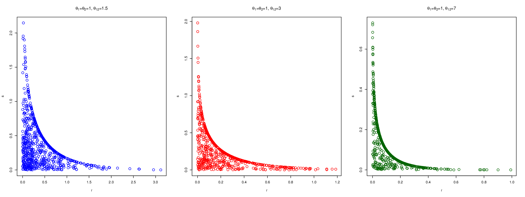
4.2 Estimation method
Here, we will estimate the parameters using maximum likelihood (ML) method.
Consider the random sample of size , namely distributed from .
Let and denote the number of observations for which and , respectively, such that . The log-likelihood function for a given sample of observations is given as
| (4.1) | |||||
where the observations are classified such that and and .
Based on the normal equations (given in the Appendix), if either of or are zero, then the ML estimator may not be unique. However, this won’t be an issue since
and
So, for moderate sample size m, the events and are rare. For the case , the resulting system of equations (normal equations given in the Appendix) cannot be solved in closed form expressions and so numerical methods are required. But, we found these methods to have less efficiency than the direct maximization of log-likelihood function in (4.1). The maximization can be performed using optim function in the R software. Initial values for optimization are derived based on global non-linear optimization package "Rsolnp" in the R software version 3.6.1. The constraints was taken into account. We found the local maximums after having different values of . So, we select the global maximum based on the following relation
| (4.2) |
4.3 Performance analysis
Next, a finite sample performance of the estimators for marginal parameters and dependence parameter is given. The performance is evaluated according to bias and mean square error (MSE) of the ML estimators introduced in the previous section. A specific sample size has been taken from and MSEs have been calculated based on 10000 iterations. The results are shown in Figure 7. Clearly, the ML estimator performs very well for small sample sizes. Evidently, after some fluctuations, the values of bias becomes more stable around zero as the sample size increases. We must note that for the MLE, global maximum was unique all the time and did not correspond to the boundary of parameter space. The computational time required to identify the global maximum after trying out all combinations of the initial values did not exceed 7 hours.

5 Application
For illustrating results, an application of the BNGM distribution to a dataset is given in this section. Mohsin et al. 2014 explored the mercury (Hg) concentration in largemouth bass. The data were collected from 53 different Florida lakes. They were used to examine the factors that influence the level of mercury concentration in bass. In specific dates, water samples were collected from the surface of the middle of each lake and the amount of alkalinity (mg/l), calcium (mg/l) and chlorophyll (mg/l) were measured in each sample. They used the average values of August and March. After that, a sample of fish was taken from each lake with sample sizes ranging from 4 to 44 fish and the minimum mercury concentration (g/g) among the sampled fish were measured. Lange et al. 1993 observed that the bio-accumulation of mercury in the largemouth bass was strongly influenced by the chemical characteristics of the lakes. Therefore, chemical substance like calcium along with minimum mercury concentration in the sampled fish is of interest. We use the proposed distribution to model these data. As Mohsin et al. 2014 stated, we have omitted the row of the data (considered as an outlier). A data summary is given in Table 1. Based on the values of and , both variables have moderate amount of dependency.
| Statistics | Mercury | Calcium |
|---|---|---|
| Minimum | 0.04 | 1.1 |
| -Quantile | 0.09 | 3.3 |
| Median | 0.25 | 12.6 |
| Mean | 0.27 | 22.2 |
| -Quantile | 0.33 | 35.6 |
| Maximum | 0.92 | 90.7 |
| SD | 0.22 | 24.93 |
| Spearman’s rho | -0.536 | |
| Kendall’s tau | -0.392 | |
| 1.36 | ||


We have fitted an exponential distribution to the marginal data which are summarized in Table 2 and illustrated in Figure 8. Clearly the marginal distributions are well fitted to the data.
| Variables | Distribution | MLE | Log-likelihood | K-S P-value |
|---|---|---|---|---|
| Mercury | Exponential | 3.573 | 14.502 | 0.195 |
| Calcium | Exponential | 0.045 | -217.309 | 0.232 |
Now, that we are sure the marginal data are exponentially distributed, we are going to fit the joint model to the data (Mercury , Calcium) and compare it with the results given in Mohsin et al. 2014. The results are given in Table 3. It is clear that the BNMO model is a better model than the BALE model given by Mohsin et al. 2014. Both models are well fitted to the data based on the Kolmogrov-Smirnov goodness-of-fit criteria. Figure 9 shows the scatter plot of Mercury versus Calcium for real data and simulated data which are generated from the fitted BNMO model.
| Model | MLE | Log-Likelihood | K-S P-value. |
|---|---|---|---|
| BNMO | -194.0028 | 0.28 | |
| BALE (Mohsin et al. 2014) | -3887.665 | 0.16 |

6 The multivariate case
In this section we present the multivariate MO model covering all degrees of dependence. Consider the independent random variables , distributed from the exponential distribution with mean . Let be the vector of dependence structure vector of all joint elements where indicates positive and states negative dependence structure for elements and . Set as following:
| (6.1) |
When , set or . In the case , put or .
The vector is distributed as the multivariate MO model covering all range of dependence. The survival function of for observations is obtained as following:
Clearly, for every , we have
with for every . So,
Note that, when , we get the well-known multivariate MO model given in Marshall and Olkin 1967. For the case where every , we get the new multivariate MO model with negative dependence structure (denoted by MNMO) as given:
| (6.2) |
where .
Example 6.1.
Consider the trivariate case () with . Then, can be obtained by
The random vector given in (6.1) can be considered as a system with three components which are subject to joint shocks ( and for ) where the shocks are likely to be distributed unequally within the pairs. The survival function of in (6.1) is
where .
The copula function gives us the raw dependence structure of a random vector that is independent from the marginal distributions. Based on the well-known Sklar theorem (see Nelsen 2007) for every random vector and copula function , we have
and consequently for the survival copula we get
The survival copula associated with the model in (6.2) is
| (6.3) |
where , , and . For the case , the copula in (6.3) gives a special case of the model in Khoudraji 1995 and Dolati et al. 2014 found some properties.
Based on Ghosh and Ebrahimi 1981, the random vector is said to be right tail decreasing in sequence (RTDS), if for all real values ,
is decreasing in . The concept RTDS establishes the negative dependence structure. On noting that a bivariate function is RR2, if for every and , it holds that
which is equivalent to . The following statement shows that the proposed model in (6.2) has negative dependence structure.
Proposition 6.2.
Let be distributed from the MNMO model in (6.2). Then, is RTDS.
Proof.
Regarding to Ghosh and Ebrahimi 1981, we know that the vector is RTDS if the corresponding multivariate survival function is RR2 in each pair of elements for fixed values of the remaining arguments. Since for every pair , we have
So, we conclude that is RR2 in each pair of elements and hence is RTDS. ∎
7 Conclusion
In real applications, a system of components are often exposed to different shocks. The amount of shocks are effective on the reliability of the system. Based on the well-known MO bivariate shock model in (1.1), it is impossible to allocate the probability of the common shock () on each of components ( and ). We have solved this issue by proposing a new MO shock model given in (2.1) for bivariate and (6.2) for multivariate cases. The MO model in (1.1) is a special case of the given model. Also, the obtained model has desirable properties such as covering positive and negative dependence structure and having closed form of stress-strength index making it useful in applications. There are not many bivariate exponential distributions with negative dependence structure and so this model is quite appealing with this regard. Having a singular component makes the new model challenging for estimating its parameters. We have given an estimation method and applied a performance analysis on the proposed estimator to see its effectiveness. The new model is used on the real data given Mohsin et al. 2014 (which is also a bivariate exponential distribution with negative structure) and we showed that our model is more promising than their model. Finally, we have proposed the multivariate case of the given model, followed by some of its properties.
8 Appendix
Let and for all :
The Normal equations for estimating parameters are as following:
| and | ||||
References
References
- Al-Mutairi et al. [2018] Al-Mutairi, D., Ghitany, M., and Kundu, D. (2018). Weighted weibull distribution: Bivariate and multivariate cases. Brazilian Journal of Probability and Statistics, 32(1):20–43.
- Balakrishnan [2018] Balakrishnan, K. (2018). Exponential distribution: Theory, methods and applications. Routledge.
- Basu and Sun [1997] Basu, A. P. and Sun, K. (1997). Multivariate exponential distributions with constant failure rates. Journal of multivariate analysis, 61(2):159–170.
- Bayramoglu and Ozkut [2014] Bayramoglu, I. and Ozkut, M. (2014). The reliability of coherent systems subjected to marshall–olkin type shocks. IEEE Transactions on Reliability, 64(1):435–443.
- Cha and Badía [2017] Cha, J. H. and Badía, F. (2017). Multivariate reliability modelling based on dependent dynamic shock models. Applied Mathematical Modelling, 51:199–216.
- Cherubini et al. [2015] Cherubini, U., Durante, F., and Mulinacci, S. (2015). Marshall-olkin distributions-advances in theory and applications. Springer Proceedings in Mathematics & Statistics, Springer International Publishing.
- Cherubini and Mulinacci [2017] Cherubini, U. and Mulinacci, S. (2017). The gumbel-marshall-olkin distribution. In Copulas and Dependence Models with Applications, pages 21–31. Springer.
- Cui and Li [2007] Cui, L. and Li, H. (2007). Analytical method for reliability and mttf assessment of coherent systems with dependent components. Reliability Engineering & System Safety, 92(3):300–307.
- Dolati et al. [2014] Dolati, A., Mohseni, S., and Úbeda-Flores, M. (2014). Some results on a transformation of copulas and quasi-copulas. Information Sciences, 257:176–182.
- Elouerkhaoui [2017] Elouerkhaoui, Y. (2017). Credit correlation: Theory and practice. Springer.
- Esary and Marshall [1974] Esary, J. D. and Marshall, A. W. (1974). Multivariate distributions with exponential minimums. The Annals of Statistics, pages 84–98.
- Fan et al. [2009] Fan, J., Nunn, M. E., and Su, X. (2009). Multivariate exponential survival trees and their application to tooth prognosis. Computational Statistics & Data Analysis, 53(4):1110–1121.
- Genest et al. [2018] Genest, C., Mesfioui, M., and Schulz, J. (2018). A new bivariate poisson common shock model covering all possible degrees of dependence. Statistics & Probability Letters, 140:202–209.
- Ghosh and Ebrahimi [1981] Ghosh, M. and Ebrahimi, N. (1981). Multivariate negative dependence. Communications in Statistics-Theory and Methods, 10(4):307–337.
- Gómez et al. [1998] Gómez, E., Gomez-Viilegas, M., and Marin, J. (1998). A multivariate generalization of the power exponential family of distributions. Communications in Statistics-Theory and Methods, 27(3):589–600.
- Joe [1997] Joe, H. (1997). Multivariate models and multivariate dependence concepts. CRC Press.
- Khoudraji [1995] Khoudraji, A. (1995). Contribution l’étude des copules et la mod’elisation de valeurs extremes multivariées. PhD thesis, PhD Thesis, Université de Laval, Québec.
- Kundu et al. [2014] Kundu, D., Franco, M., and Vivo, J.-M. (2014). Multivariate distributions with proportional reversed hazard marginals. Computational Statistics & Data Analysis, 77:98–112.
- Kundu and Gupta [2013] Kundu, D. and Gupta, A. K. (2013). Bayes estimation for the marshall–olkin bivariate weibull distribution. Computational Statistics & Data Analysis, 57(1):271–281.
- Kundu and Gupta [2009] Kundu, D. and Gupta, R. D. (2009). Bivariate generalized exponential distribution. Journal of Multivariate Analysis, 100(4):581–593.
- Lange et al. [1993] Lange, T. R., Royals, H., and Connor, L. L. (1993). Influence of water chemistry on mercury concentration in largemouth bass from florida lakes. Transactions of the American Fisheries Society, 122(1):74–84.
- Li and Pellerey [2011] Li, X. and Pellerey, F. (2011). Generalized marshall–olkin distributions and related bivariate aging properties. Journal of Multivariate Analysis, 102(10):1399–1409.
- Lin et al. [1993] Lin, H.-H., Chen, K., and Wang, R.-T. (1993). A multivariant exponential shared-load model. IEEE Transactions on Reliability, 42(1):165–171.
- Lindskog and McNeil [2003] Lindskog, F. and McNeil, A. J. (2003). Common poisson shock models: Applications to insurance and credit risk modelling. ASTIN Bulletin: The Journal of the IAA, 33(2):209–238.
- Marshall and Olkin [1967] Marshall, A. W. and Olkin, I. (1967). A multivariate exponential distribution. Journal of the American Statistical Association, 62(317):30–44.
- Mohsin et al. [2014] Mohsin, M., Kazianka, H., Pilz, J., and Gebhardt, A. (2014). A new bivariate exponential distribution for modeling moderately negative dependence. Statistical Methods & Applications, 23(1):123–148.
- Mohtashami-Borzadaran et al. [2020] Mohtashami-Borzadaran, H., Jabbari, H., and Amini, M. (2020). Bivariate marshall–olkin exponential shock model. Probability in the Engineering and Informational Sciences, pages 1–21.
- Nelsen [2007] Nelsen, R. B. (2007). An introduction to copulas. Springer Science & Business Media.
- Raftery [1984] Raftery, A. E. (1984). A continuous multivariate exponential distribution. Communications in Statistics-Theory and methods, 13(8):947–965.
- Shih and Emura [2016] Shih, J.-H. and Emura, T. (2016). Bivariate dependence measures and bivariate competing risks models under the generalized fgm copula. Statistical Papers, pages 1–18.
- Tawn [1990] Tawn, J. A. (1990). Modelling multivariate extreme value distributions. Biometrika, 77(2):245–253.