Cosmological models of generalized ghost pilgrim dark energy (GGPDE) in the gravitation theory of Saez-Ballester
PRIYANKA GARG1, ARCHANA DIXIT2, ANIRUDH PRADHAN3
1,2,3Department of Mathematics, Institute of Applied Sciences & Humanities, GLA University,
Mathura -281 406, Uttar Pradesh, India
1E-mail:pri.19aug@gmail.com
2E-mail: archana.dixit@gla.ac.in
3E-mail:pradhan.anirudh@gmail.com
Keywords. LRS Bianchi type-I metric; Ghost Pilgrim dark energy;
time-dependent deceleration parameter; Saez-Ballester theory.
PACS Nos 98.80.Jk; 95.36.+x; 98.80.-k
Abstract
We are studying the mechanism of the cosmic model in the presence of GGPDE and matter in LRS Bianchi type-I space-time by the utilization of new holographic DE in Saez-Ballester theory. Here we discuss all the data for three scenarios, first is supernovae type Ia union data, second is SN Ia data in combination with BAO and CMB observations and third is combination with OHD and JLA observations. From this, we get a model of our universe, where its transit state from deceleration to acceleration phase. Here we have observed that the results yielded by cosmological parameters like (energy density), EoS (equation of state), squared speed of sound , and plane is compatible with the recent observational data. The trajectories in both thawing and freezing regions and the correspondence of the quintessence field with GGPD dark energy are discussed. Some physical aspects of the GGPDE models are also highlighted.
1 Introduction
Nowadays it is accepted by almost every scientist in cosmology and relativity field that the cosmos is expanding till 1998, and
the expansion rate is decreasing, because of gravity following up on the matter. In 1998 and following years, many groups of
astronomers [1, 2, 3, 4, 5, 6], in their search for the estimation of the universe expansion rate have
observed some surprising results. These groups, in view of SN Ia observations, have estimated the separations and predicted
the accelerated expansion of the cosmos, which is probably going to continue forever. It is anticipated by these observations
that something is responsible for this acceleration. To answer this, the cosmological constant , which can be the
best candidate for dark energy (DE). Researchers [7, 8] have discussed locally rotationally symmetric ghost pilgrim
dark energy cosmological models. In the Saez-Ballester theory of gravitation Bianchi type-II, VIII, and IX dark energy models have
been discussed by [9]. Many authors [3, 10], have observed the cosmological observation that the expansion
of the universe is accelerating.
To rectify the problem of DE, various DE models such as phantom, tachyon, quintessence, and Chaplying gas have been proposed by
cosmologists from time to time. The cosmology scientist usually accepts that a type of repulsive force that
works as anti-gravity generated somewhere in the range of billion years back is the reason for speeding up the expansion of
the universe. This obscure physical entity is named as ‘dark energy’. Along with this, various researchers considered many alternative
candidates as a possible source of dark energy in different scenario [11, 12, 13, 14] in the Saez-Ballester theory.
Higher-dimensional cosmic models have been discussed by [15, 16, 17, 18].
Other than these research, a few cosmologists have studied holographic DE models as other options to DE causing late-time speeding
expansion of the universe [19, 20, 21, 22, 23, 24, 25, 26, 27, 28, 29, 30]. The hypothesis, that
phantom-like DE has an adequate resistant force to cause the formation of black hole in our universe later, is the base of the
proposal of pilgrim dark energy. Depending on the assumption of the generalized ghost version of the pilgrim dark energy this
phenomenon has been explored. We found that the parameter (EoS) varies in both quintessence and phantom regions. Here we use
linearly varying deceleration parameter (LVDP) to test the GGPD dark energy model in the SB scalar-tensor theory of gravity.
We discuss the EoS parameter, squared speed of sound , trajectories and planes to analyze the
results [31]. Nowadays, due to the global property of the Universe the holographic dark energy has attracted much attention.
This model depends on the holographic principle [32, 33, 34, 35, 36, 37, 38, 39].
Furthermore, a model of dark energy named PDE (pilgrim dark energy) has been introduced by [40], and it is based on the fact
that the strong repulsive force of dark energy can avoid the formation of the black hole. Instead of other types of DE, the
phantom DE can play an important role. This argument coincides with the concept given by [41] which says that the mass
of black holes tends to zero in the phantom energy universe approaching the Big Rip. (energy density) of GGPDE is
discussed and given in [42, 43]. Cosmological model in theory of gravity are analyzed in [44, 45].
The detail expression for it is given by Eq. (13) in Sect. .
In the non-flat FRW universe has studied the analysis of GGPDE in [46]. The GGPDE of dark energy is also investigated in [47].
In general relativity, some Bianchi type GGPDE models have been studied by [48, 49]. Currently [50] have studied
Bianchi-type- GGPDE model. Researcher [51] have discussed the cosmological implication
of interacting PDE models (with Hubble, Granda-Oliveros and generalized ghost cutoffs) CDM in fractal cosmology by taking the
flat universe. The GPDE model in gravity with flat FRW universe have studied in [52]. Interacting GGDE in a non-flat
universe has been discussed by [53]
In this paper, our aim is to investigate the LRS Bianchi type-I GGPDE model in the Saez-Ballester theory of gravitation. The paper has the following structure. Sect. , presents deviation of field equations in Saez-Ballester’s theory. In Sect. , we obtained the metric and field equations for Bianchi type-I space times. In Sect. , we describe calculations of some other physical and kinematic parameters. Interpretation of the results obtained is written in Sect. . In Sect. , we deal the the stability analysis of the solution. State-finder p () have been obtained in Sect. . Sound speed is discussed in Sect. . The analysis of in Sect. . Correspondence of quintessence field in Sect. . In the last part Sect. , conclusion and the description are given.
2 Explicit field equations in Saez-Ballester theory
The field equations founded by Saez-Ballester [1] for the combined scalar and tensor fields are:
| (1) |
and the equations which are satisfied by (scalar field) :
| (2) |
In addition the conservation equation is
| (3) |
Here, is the Ricci scalar, is the Ricci tensor, and are arbitrary dimensionless constants and = C = in
the relativistic units.
Now, we define and which are energy-momentum tensors for matter and holographic dark energy such as
| (4) |
| (5) |
Here is the holographic dark energy, is the energy densities of matter and is the pressure of holographic
dark energy.
Now LRS Bianchi type-I metric takes the form
| (6) |
where and are time dependent functions.
Now using Eqs. (1), (2), (4), (5) and co moving coordinates for the metric (6) form the following equations
| (7) |
| (8) |
| (9) |
| (10) |
Here overhead dot indicates differentiation with respect to .
Here the EoS parameter of dark energy is .
The conservation equation of the matter and dark energy is
| (11) |
3 Solutions of the field equations
Now, we solve the field equations Eqs. (7)- (10), which are a system of four independent field equations in six unknowns
parameters and . Therefore, to obtain explicit solutions of the system,
For solving the above highly non-linear differential equations we have required the following physically significant conditions, which
are relating to these parameters.
We assume that the expansion scaler () is proportional to shear scalar (). The condition leads to , which yields [54]
| (12) |
The motivation behind assuming this condition is given [55].
The energy density of GGPDE defined by [42]
| (13) |
where is the Hubble parameter, = is the reduced Plank mass, is PDE parameter, and
, are two arbitrary dimensionless parameters.
Motivated by the recent observational data, we consider the deceleration parameter as a linear function of Hubble parameter as [56]
| (14) |
Here and are arbitrary constants.
Solving Eq. (14), , the various authors [56, 57, 58, 59] obtained the solution as:
| (15) |
where is an integrating constant. Recently this Eq. (15) is used by many authors [56, 57, 58, 59].
We have found the value of deceleration parameter from Eq. (19)
| (16) |
As it has been observed that the expansion rate of the universe is time dependent instead of being constant. So we will use ,
for which we find the time dependent value of DP and not as it results into constant DP .
The average scale factor for the metric (6) is define as .
Therefore, the geometry of the metric comes out to be
| (19) |
where and are constants of integration.
Now we find the energy density of GGPDE from (13) as
| (21) |
From Eqs. (9), (17), (18), (20) and (21) we find the energy density of the matter as
| (22) |
The expression for pressure of holographic dark energy is obtained as:
| (23) |
The density parameter is given by
| (25) |
which is equal to
| (26) |
4 Experimental data and calculations of parameters
From Eq. (14), we have , where and are the present values of DP and Hubble parameter respectively.
Also, we have , so that . Using , we
can get . Solving it for , we have .
Here three cases has been considered which is based on three different data:
Case I: Based on supernovae type la union data
Now, taking and [60], we obtain . For these values and , we get .
Case II: Based on SN la data in combination with BAO and CMB observations
Taking and [61] , we obtain . For these values and , we get .
Case III: Based on current data in combination with OHD and JLA observations
Taking and [62], we obtain . For these values and , we get .
| Reference | ||||
|---|---|---|---|---|
| [60] | ||||
| [61] | ||||
| [62] |
In this paper we have drawn all the figures for these different values of (, ) as (0.003658, 0.000084), (0.0062, 0.00001),
and (0.0069, 0000083) respectively.
The Hubble parameter , scalar expansion , shear scalar and the average anisotropy parameter are calculated for our model which is defined as:
| (27) |
| (28) |
| (29) |
| (30) |
5 Results and discussions
Figure depicts cosmological model with DP () versus time . It can be observe that for = and
= , our models are only in accelerating phase, but for = and = , the model shows a
transition phase from +ve to -ve deceleration parameter i. e. our model is transforming from (deceleration) to
(acceleration) phases. Similarly for the current data and models is decelerating to the
accelerating phase transforming. Since DP () value lies between the range
and the expansion of the current universe in accelerating are exposed by SNe 1a data. So
the value of the decelerating parameter is consistent with recent observations.
The value of scale factor ( ) in the form of is , where is the current value of scale factor.
From Eq. (19), we find . And we also obtain the value of
in term of redshift , i.e. from . Using this value
in Eq. (20), we obtain .
For our derived model variation of redshift versus (cosmic time) is demonstrate by figure 1(b). In this figure we have seen that
for this value redshift is a monotonic decreasing with increase of . So it can be say that for our model derived
starts with a small positive value at equal to and tends to as tends to .
Figure 1(c) shows plane for generalized -parametrization given by for three cases
of i.e.( = , = , = , = and = , = )
and we get the value of . For plot the graph we use these values.
In the figure we have discovered that expansion undergoes a smooth transition from a decelerated stage to accelerated stage and
as . Currently, [63, 64] have discovered the change redshift from decelerating to accelerating in
modified gravity cosmology. SNe type Ia dataset has given the progress from past deceleration to ongoing acceleration.
More recently, in 2004 the HZSNS team have found at c.l. [4].
It is improved in 2007 to at c.l. [5]. SNLS
[65] compiled by [66], provide a progress redshift in improved
agreement with the flat CDM model ().
Moreover the reconstruction of is done by the joined , which have obtained the transition redshift and within [67]. which are seen as well consistent with past outcomes [68, 69, 70, 71, 72] including the expectation . Another limit of transition redshift is (, joint examination ) [73].
(a)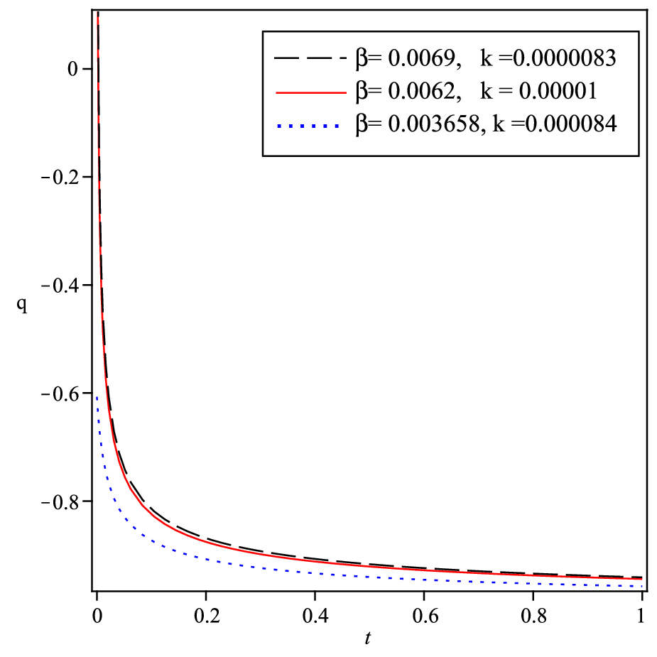 (b)
(b)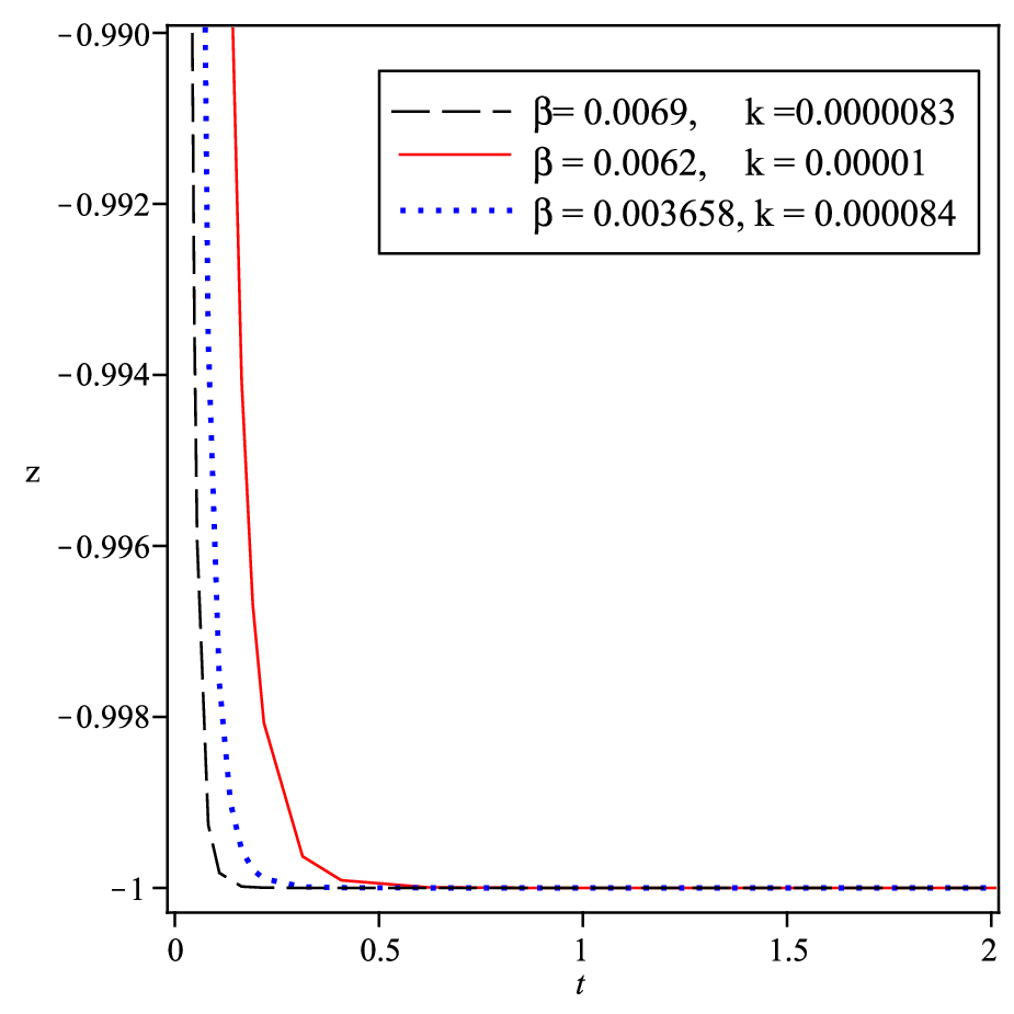
(c)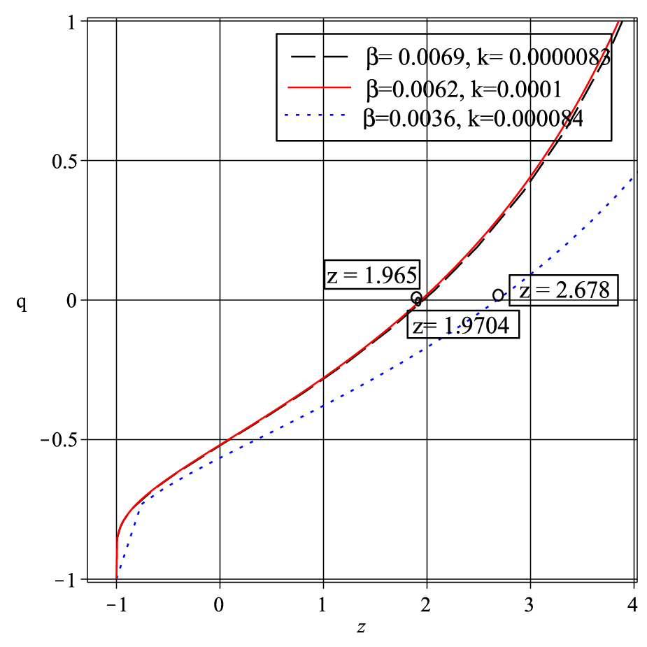 (d)
(d)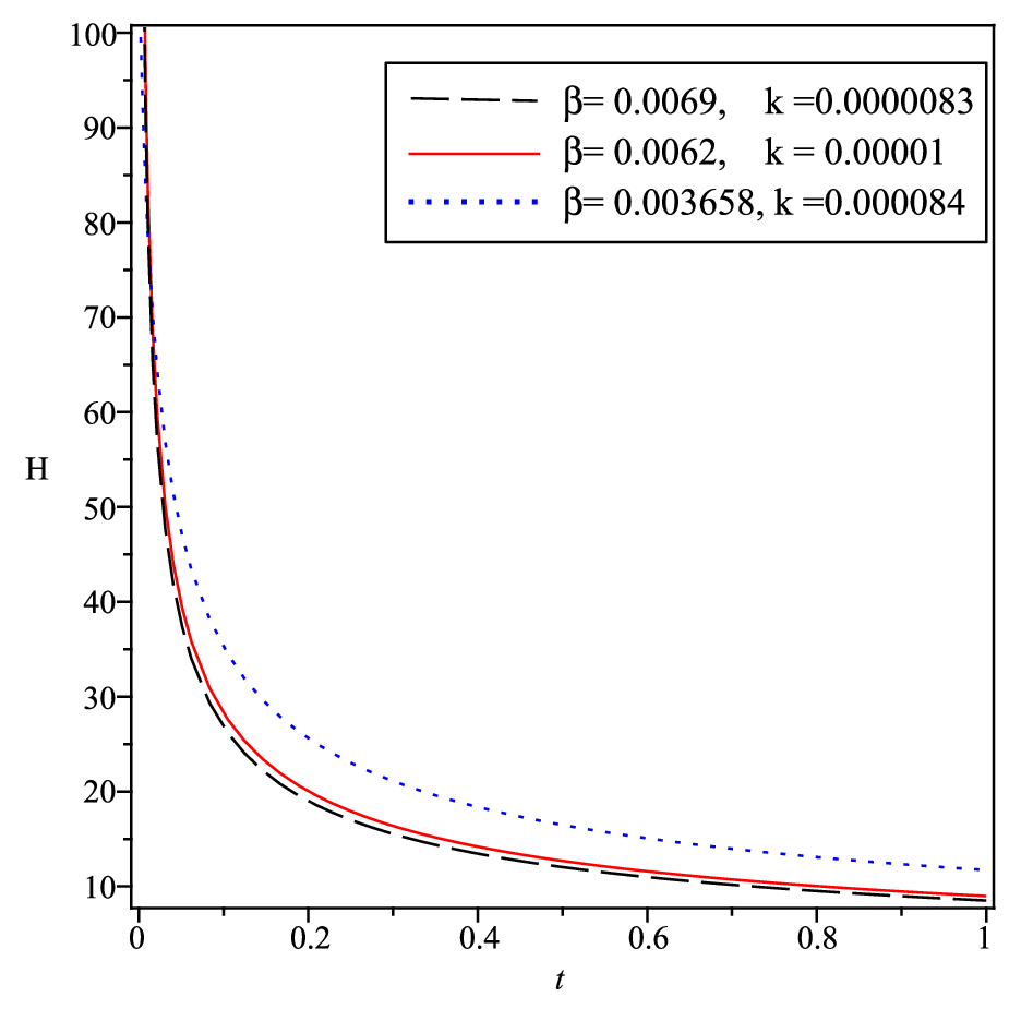
From the figure it is clear that the transition redshift from decelerated to accelerated expansion occurs at
, and (see Fig. ) for above three cases which are found to be well consistent
with the Type Ia supernovae Hubble diagram, including the farthest known supernova SNI997ff at [74, 75]).
Figure depicts between the Hubble parameter and time. We observed that as as per theoretical desire.
(a)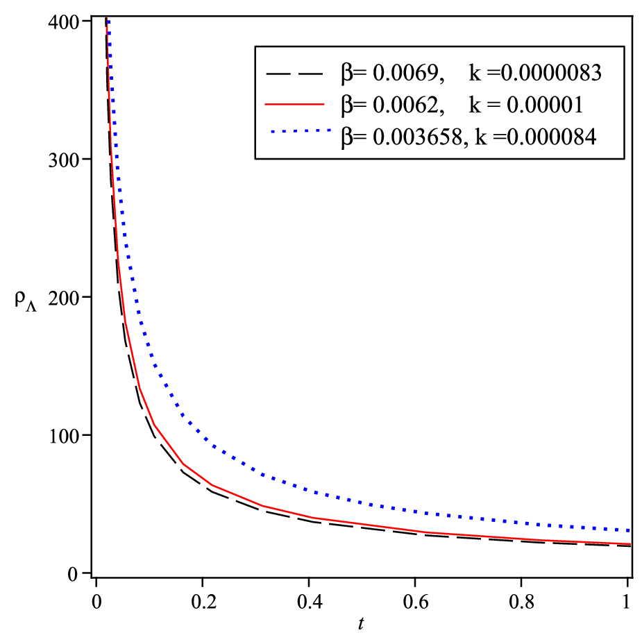 (b)
(b)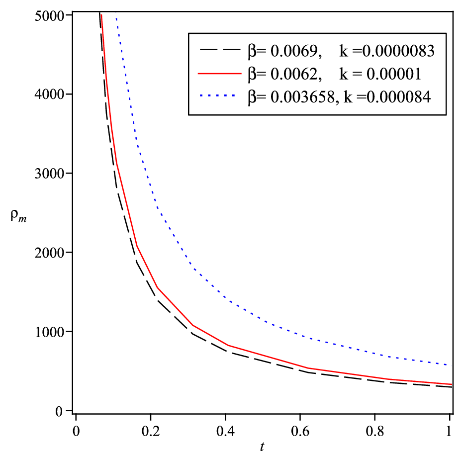
We observe that from Eq. (25) and it’s corresponding figure , shows that for all three cases remains positive during the cosmic evolution. Similarly from Eq. (26) and it’s corresponding figure , it indicates that the energy density of matter decreases with increase of time and it also remains positive for all values of and during the cosmic evolution. We can see first it decreased sharply and then gradually and approach to a small positive values at the present epoch. and tends to as . Since decrease in density implies the increase in volume i.e. our derived model represents the expansion of the universe.
(a)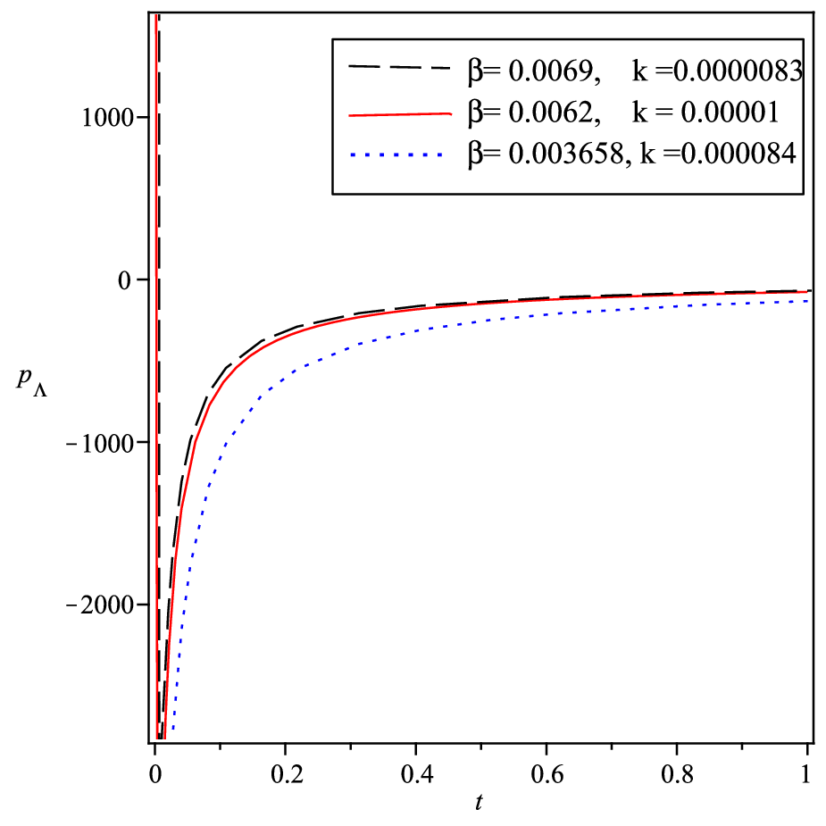 (b)
(b)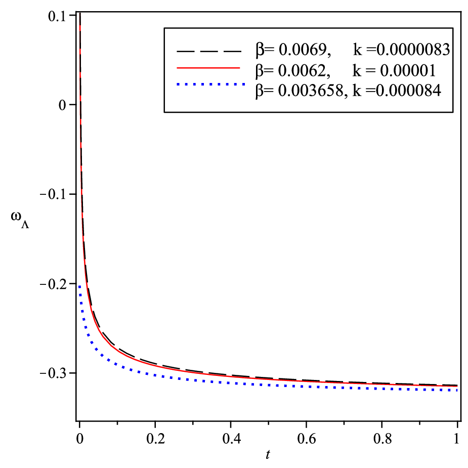
Figure depicts pressure versus time . It is observed that the value of isotropic pressure was positive in the
beginning. Later it decreased rapidly and then it remained negative throughout evolution. This negative pressure put the equation of state
, as prescribed by recent observations and it may be a cause of the accelerated expansion of
the universe. Figure demonstrate the equation of state parameter for all three observational value.
From Eq. (28) and its corresponding figure , it is clearly shown that for all three data firstly EoS
parameter was positive then decreased sharply and approach to a small negative value at the present epoch. The EoS
parameter of DE may begin in phantom or quintessence region and tends to by
exhibiting various patterns as increases. Here is less than so there is a phantom region. i.e.
evolves with negative and its range is in nice agreement with large scale structure data [76].
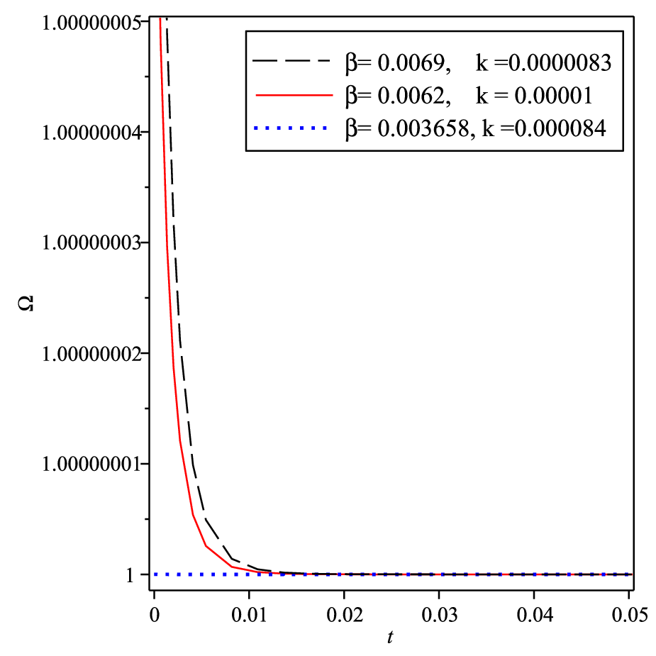
Figure shows the graph of versus for all three values of (). We observe that approaches close to as
i.e. the total energy density of GGPDE models at present is .
Jerk is the rate of change of acceleration; that is, the time derivative of acceleration. Many authors [77, 78] have indicated
the significance of jerk as a tool to reconstruct the cosmological models. Recently, [79, 80] have discussed the parametrization
of time evolving jerk parameter models.
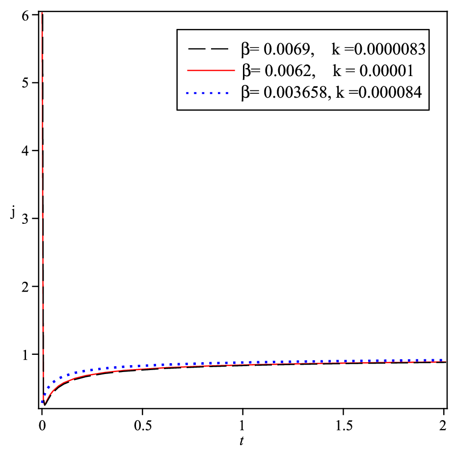
We hereby define the cosmic Jerk parameter such as:
| (31) |
| (32) |
Figure demonstrate that firstly the graphs decrease rapidly for all three value & ; & , and & then approach to through the evolution history i.e. the best suitable value of is very close to is showed by this figure and it clearly indicates that the model is extremely close to CDM model. A well known constrained value of jerk parameter is found by statistical analysis with different observational data sets like BAO (baryon acoustic oscillation data), SNe (Ia supernova data) and OHD (observational Hubble parameter data). A well known constrained value of jerk parameter is found by statistical analysis with different observational data sets like BAO (baryon acoustic oscillation data), SNe (Ia supernova data) and OHD (observational Hubble parameter data) and the model remains at very close proximity of the CDM.
6 Squared sound speed
Many authors [81, 82] have examined the speed of sound constraints of dynamic DE models with EoS parameter varying in
time and concluded that the speed of the sound constraint of DE is very low. If the speed of sound lies between zero and 1, the system
is stable.
Now for any fluid, the adiabatic square sound speed is described as . Besides the positivity of , the condition of causality must satisfied. Causality means the speed of sound should not surpass the speed of light. Since we use relativistic units where = = , the speed of sound should be within the range .
| (33) |
(a)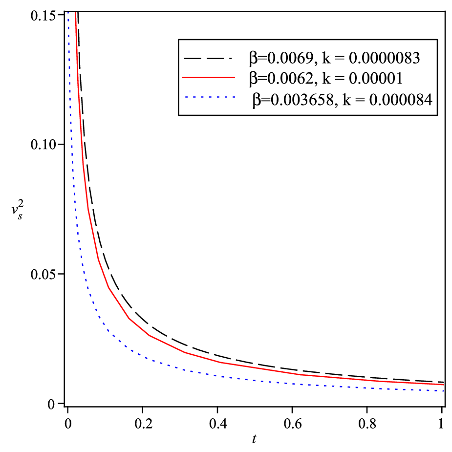
Figure depict the plots of speed of sound with time for all three values of and . We observe that throughout the evolution of the universe. From the figure, it is sorted out that throughout the universe evolution sound speed remains less than light velocity ().
7 The analysis
Caldwell and Linder [83] implemented a plane analysis of . This analysis is a utile shaft
for separating vDE models by trajectories on their planes. The method is also applied to the quintessence model that leads to two forms
of its plane, i.e. the area belongs to the
region refers to the thawing region while the area below the region indicates the freezing region.
Later this analysis was extended by many researchers to other dynamic DE models [84, 85, 86, 87]. Clearly, a fixed point
at is the CDM model in the phase space. To discuss GGPDE model, here we use this analysis.
On differentiating Eq. (24) w.r.t. and find the value of
as
| (34) |
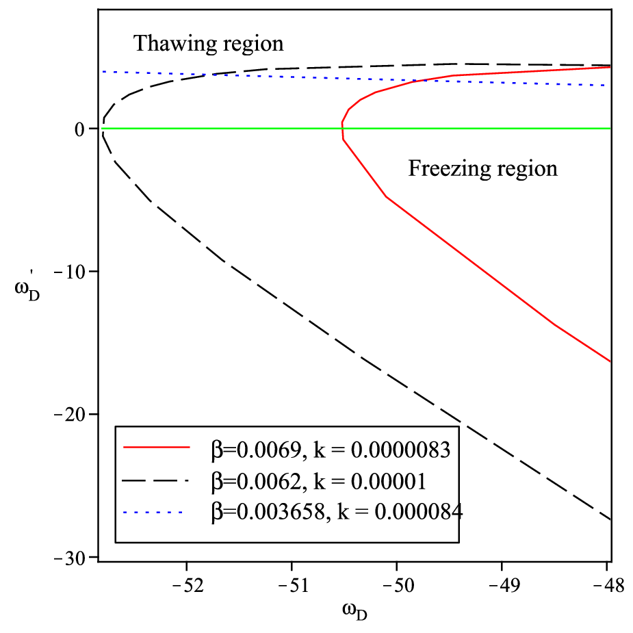
We constructed the plane by plotting versus as shown in Fig. . It can be observed that the curves lead to both freezing and thawing regions for three values of parameter and . Nevertheless, the trajectories differ for the supernova Ia union data in the thawing region and for the BAO CMB observations and OHD JLA observation curves correspond to both the freezing and thawing areas. Nevertheless, our model’s trajectories differ mostly in the freezing zone, as indicated by observational data (the expansion of the universe is comparatively more accelerated in the freezing area).
8 Correspondence of quintessence field in GGPDE
In the presence of non-relativistic matter represented by a barotropic perfect fluid, let us consider quintessence. The quintessence field action is given in [88]
| (35) |
where is the reduced Planck mass, is the metric whereas is the metric determinant and is the scalar Ricci. In the
above, is the action standard field, is the potential for the quintessence field and is the covariant
derivative of .
By varying the action given in Eq. (35) with respect to the metric and respectively we obtain,
| (36) |
| (37) |
On solving Eqs. (36) and (37), we obtain potential versus cosmic time .
| (38) |
and scalar field versus time is
| (39) |
(a)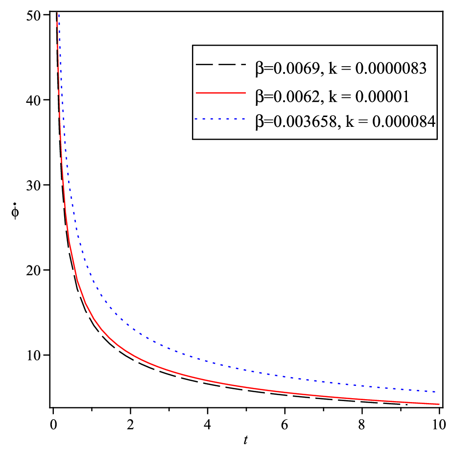 (b)
(b)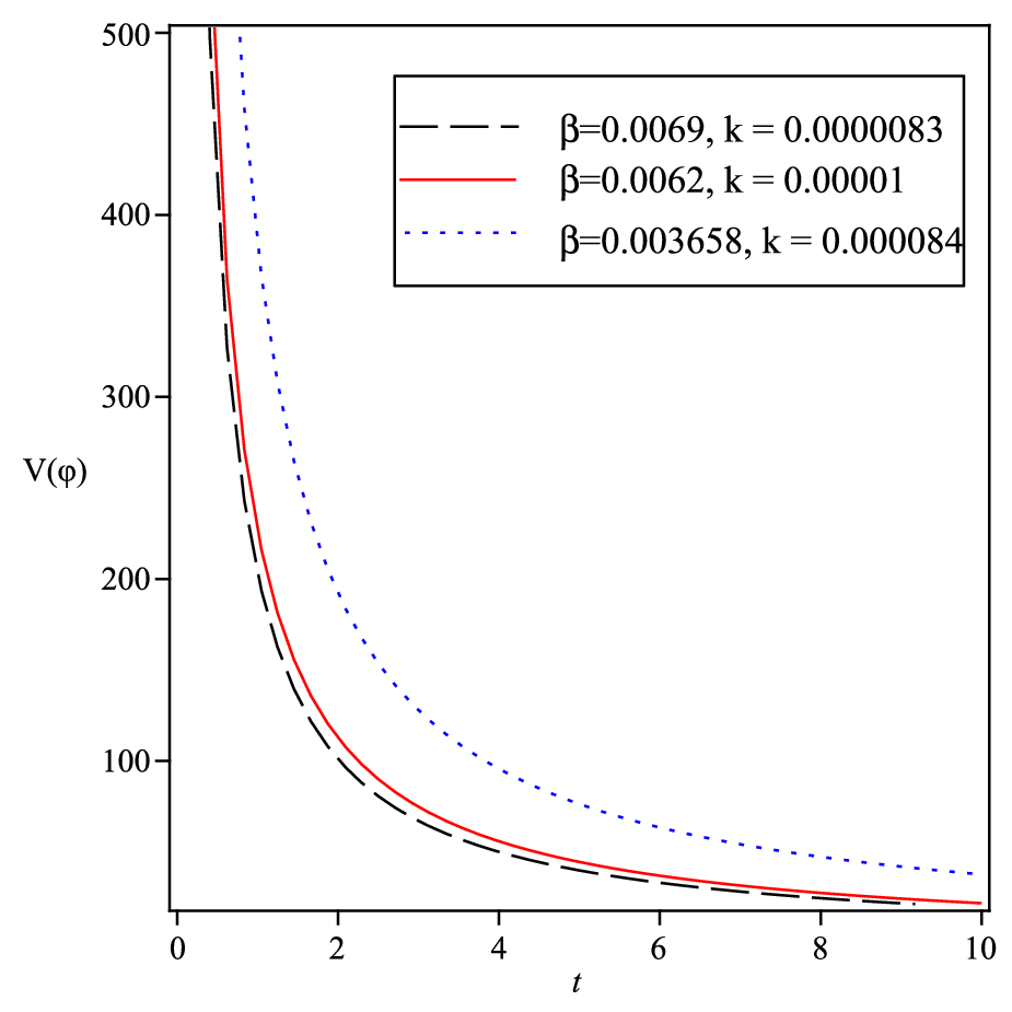
A canonical scalar field describe the quintessence model.
A slowly varying potential of scaler field can lead to the accelerating Universe.
This method is close to slow inflation in the early Universe. But the difference is that it is not possible to ignore non-relativistic matter
(dark matter and baryons) to accurately explain the nature of DE.
Figure shows the graph of scalar field with time for all three values of and . Scalar field decreases through the evolution of time and tends to small positive value at the present epoch. Figure depicts potential of scalar field that correspond to LRS Bianchi type-I GGPDE model, which is also decreasing function of time
9 Concluding remarks
A new LRS Bianchi type-I generalized ghost pilgrim DE anisotropic universe with time dependent DP and time dependent EoS parameter has been explored by new idea.
Here we have considered two assumptions: (i) (shear scalar) (scalar expansion) and (ii) the DP as
a linear function of ( Hubble parameter).
There are following main features of the model:
- •
For different purposes, like in analysis of jerk parameter, correspondence with various scalar field models, thermodynamics laws, the evolution of our universe by extracting different cosmological parameters, the generalized ghost dark energy model play a very important role. In different modified theories, various cosmological aspects of this model have been also addressed. It should be mentioned here that (energy density of matter) and (the proper energy density), are positive in the deduced model.
- •
The anisotropic parameter is a constant and is non-zero for . ie. our model is anisotropic and may attain isotropy if .
- •
The interacting scenario of generalized ghost dark energy with CDM has been studied and cosmological parameters like jerk parameter, total energy density and equation of state parameter (EoS) have been evaluated by us. For three different well-known values of and , equation of state parameter (EoS) of PDE parameter has been explored. is in the phantom region of our universe for all three observational values of and .
- •
The GGPDE gives the dynamics of given by Eq. (30). In this derived model, is obtained as time dependent which is a positive decreasing with time and approach to at present epoch (Figure ).
- •
It is observed that the best suitable value of jerk parameter is very close to at present time (Figure ). This shows that our GGPD model is very close to the CDM model.
- •
The model represents that , and diverge at ), but the volume becomes unity at ). Hence, the GGPD model starts expanding with a big bang singularity at ). It may be observed that when tends to , the volume becomes .
- •
The GGPD model represents an expanding, shearing, non-rotating and transit (from decelerating to accelerating) Universe.
- •
The squared sound speed trajectories demonstrate positive behavior throughout the evolution and model stability are also discussed in (Fig.).
- •
For our GGPD model, we also developed the plane in (Fig.) correspond to both thawing regions and freezing regions.
. - •
Nevertheless, our model’s trajectories differ mostly in the freezing region, as indicated by observational data (the expansion of the universe is comparatively more accelerated in the freezing region).
- •
We also observed the quintessence correspondence with a scalar field and potential in (Fig.). For many different potentialities, the dynamics of quintessence in the presence of non-relativistic matter have been studied in detail [83, 88, 89, 90, 91]. This result is a good agreement with the current scenario of the universe.
Hence, our constructed model and their solutions are physically acceptable. Therefore, for the better understanding of the characteristics within the framework of consistency GGPD models, the solution demonstrated in this paper may be helpful.
References
- [1] D Saez and V J Ballester, Phys. Lett. A 113, 467 (1986)
- [2] M S Berman, Il Nuovo Cimento B 74, 182 (1983)
- [3] A G Reiss et al, Astrophys. J. 116, 1008 (1998)
- [4] S Perlmutter et al, Astrophys. J. 517, 565 (1999)
- [5] D N Spergel et al, Astrophys. J. Suppl. 148, 175 (2003)
- [6] M Tegmark et al, Astrophys. J. 606 702 (2004)
- [7] V U M Rao, M V Santhi, T Vinutha and G Sreedevi Kumari, Int. J. Theor. Phys. 51, 3303 (2012)
- [8] V U M Rao, K V S Sireesha and P Suneetha, African Rev. Phys. 7, 0054 (2012)
- [9] V U M Rao, K V S Sireesha and D Neelima, ISRN Astron. Astrophys. 2013 Article ID 924834, 11 (2013)
- [10] C L Bennett et al, Astrophys. J. Suppl. Ser. 148, 1 (2003)
- [11] V U M Rao, T Vinutha and K M Vijaya Santhi, Astrophys. Space Sci. 314, 213 (2008)
- [12] V U M Rao, V Santhi and T VinuthaK, Astrophys. Space Sci. 314, 27 (2008)
- [13] R L Naidu et al, Int. J. Theor. Phys. 51, 1997 (2012)
- [14] R L Naidu et al, Astrophys. Space Sci. 338, 333 (2012)
- [15] V U M Rao and D Neelima, Astrophys. Space Sci. 345, 427 (2013)
- [16] V U M Rao, K V S Sireesha and B J M Rao, Prespacetime J. 5, 772 (2014)
- [17] V U M Rao, D C Papa Rao and D R K Reddy, Astrophys. Space Sci. 357, 77 (2015)
- [18] V U M Rao and V Jayasudha, Astrophys. Space Sci. 358, 8 (2015)
- [19] O Akarsu and C B Kilinc, Astrophys. Space Sci. 326, 315 (2010)
- [20] O Akarsu and C B Kilinc, Gen. Relativ. Gravit. 42, 763 (2012)
- [21] R Zia, U K Sharma and D C Maurya, New Astronomy 72, 83 (2019)
- [22] A K Yadav, Astrophys. Space Sci. 335, 565 (2011)
- [23] A Pradhan, R Jaiswal, K Jotania and R K Khare, Astrophys. Space Sci. 337, 401 (2012)
- [24] T Singh and R Chaubey, Pramana-J. Phys. 71, 447 (2008)
- [25] B Saha and A K Yadav, Astrophys. Space Sci. 341, 651 (2012)
- [26] K S Adhav et al, Astrophys. Space Sci. 332, 497 (2011)
- [27] S Sarkar and C R Mahanta, Int. J. Theor. Phys. 52, 1482 (2013)
- [28] S Sarkar, Gen. Relativ. Gravit. 45, 53 (2013)
- [29] S Sarkar, Astrophys. Space Sci. 349, 985 (2014)
- [30] S Sarkar, Astrophys. Space Sci. 351, 361 (2014)
- [31] G Varshney, U K Sharma and A Pradhan, New Astronomy 70, 36 (2019)
- [32] L Susskind, Jour. Math. Phys. 36 (1995) 6377
- [33] S D H Hsu, Phy. Lett. B 594, 13 (2014)
- [34] M Li, Phys. Lett. B 603, 15 (2004)
- [35] A Cohen et al, Phys. Rev. Lett. 82, 4971 (1999)
- [36] M R Setare, J Zhang and X Zhang, JCAP 03, 007 (2007)
- [37] M Malekjani, A K Mohammadi and N N Pooya, Astrophys. Space Sci. 332, 515 (2011)
- [38] Y Aditya and D R K Reddy, Astrophys. Space Sci. 363, 207 (2018)
- [39] V U M Rao, G Suryanarayana and U D Prasanthi, Bulletin Math. Statis. Res. 5, 48 (2017)
- [40] H Wei, Class. Quantum Grav. 29, 175008 (2012)
- [41] E Babichev et al, Phys. Rev. Lett. 93, 021102 (2004)
- [42] M Sharif and A Jawad, Astrophy. Space Sci. 351, 321 (2014)
- [43] C R Mahantaa and N Sarmab, New Astronomy 57, 70 (2017)
- [44] D D Pawar and S P Shahareab, New Astronomy 75, 101318 (2020)
- [45] M S Singh and S Singh, New Astronomy 72, 36 (2019)
- [46] A Jawad, Eur. Phys. J. C 74, 3215 (2014)
- [47] A Jawad, V Debnath and F Batool, Commun. Theor. Phys. 64, 590 (2015)
- [48] M V Santhi et al, Astrophys. Space Sci. 361, 142 (2016)
- [49] M V Santhi et al, Int. J. Theor. Phys. 56, 362 (2017)
- [50] V U M Rao and U Y D Prasanthi, Can. J. Phys. 95, 554 (2017)
- [51] A Jawad, S Rani, I G Salako and F Gulshan, Int. J. Mod. Phys. D 26, 1750049 (2017)
- [52] M Sharif and K Nazir, Mod. Phys. Lett. A 31, 1650148 (2016)
- [53] E Ebrahimi, A Sheykhi and H Alavirad, Cent. Europ. Jour. Phys. 11, 949 (2013)
- [54] C B Collins and J Wainwright, Phys. Rev. D 27, 1209 (1983)
- [55] K S Thorne, Astrophys. J. 148, 51 (1967)
- [56] P Garg, R Zia and A Pradhan, Int. J. Geom. Methods Mod. Phys. 16, 1950007 (2019)
- [57] R K Tiwari, R Singh and B K Shukla, African Rev. Phys. 10, 0048 (2015)
- [58] U K Sharma, R Zia, A Pradhan and A Beesham, Res. Astron. Astrophys. 19, 4 (2018)
- [59] R K Tiwari, A Beesham and B K Shukla, Int. J. Geom. Methods Mod. Phys. 15, 1850189 (2018)
- [60] J V Cunha, Phys. Rev. D 79, 047301 (2009)
- [61] R Giostri et al, J. Cosmol. Astropart. Phys. 03, 027 (2012)
- [62] H Amirshaschi and S Amirhashchi, arXiv:1802.04251 [astro-ph.co] (2018)
- [63] S Capozziello, O Farooq, O Luongo and B Ratra, Phys. Rev. D 90, 044016 (2014)
- [64] S Capozziello, O Luongo and E N Saridakis, Phys. Rev. D 91, 124037 (2015)
- [65] P Astier et al, Astron. Astrophys. 447, 31 (2006)
- [66] T M Davis et al, Astrophysical J. 666, 716 (2007)
- [67] A A Mamon, Mod. Phys. Lett. A 33, 1850056 (2018)
- [68] R Nair et al, JCAP 01, 018 (2012)
- [69] A A Mamon and S Das, Int. J. Mod. Phys. D. 25, 1650032 (2016)
- [70] O Farooq and B Ratra, Astrophys. J 766, L7 (2013)
- [71] J Magana et al, JCAP 10, 017 (2014)
- [72] A A Mamon, K Bamba and S Das, Eur. Phys. J. C 77, 29 (2017)
- [73] J A S Lima, J F Jesus, R C Santos and M S S Gill, arXiv: 1205.4688v3[astro-ph.CO] (2012)
- [74] A G Riess et al, Astrophys. J. 560, 49 (2001)
- [75] L Amendola, Not. R. Mon. Astron. Soc. 342, 221 (2003)
- [76] E Komatsu et al, Astrophys. Jour. Suppl. Ser. 180, 330 (2009)
- [77] V Sahni, T D Saini, A A Starobinsky and U Alam, Jour. Exper. Theor. Phys. Lett. 77, 201 (2003)
- [78] R D Rapetti, S W Allen, M A Amin and R D Blandford, Mon. Not. Roy. Astron. Soc. 375, 1510 (2007)
- [79] A Mukherjee and N Banerjee, Phys. Rev. D 93, 043002 (2016)
- [80] Z X Zhai, M J Zhang, Z-S Zhang, X-M Liu, and T-J Zhang, Phys. Lett. B 727, 8 (2013)
- [81] J Q Xia, Phys. Rev. D 73, 063521 (2006)
- [82] G B Zhao et al, Phys. Rev. D 72, 123515 (2005)
- [83] R R Caldwell, E V Linder, Phys. Rev. Lett. 95, 141301 (2005)
- [84] T Chiba, Phys. Rev. D 73, 063501 (2006)
- [85] Z K Guo et al. Phys. Rev. D 74, 127304 (2006)
- [86] M Malekjani, A K Mohammadi, Int. J. Theor. Phys. 51, 3141 (2012)
- [87] V Sahnia, A Shafielooa and A A Starobinsky, arxiv:0807.3548v3 [astro-ph] (2008)
- [88] S Tsujikawa, Class. Quant. Grav. 30, 214003 (2013)
- [89] E J Copeland, A R Liddle and D Wands, Phys. Rev. D 57, 4686 (1998)
- [90] D L Macorra and G Piccinelli, Phys. Rev. D 61, 123503 (2000)
- [91] E V Linder, Phys. Rev. D 73, 063010 (2006)