跳到论文正文
W Papers独立论文阅读器 arXiv:2004.11100 论文正文 计算阅读时间 · 0%
引用这篇论文根据当前论文元数据生成,正式投稿前建议核对。


License: arXiv.org perpetual non-exclusive license
arXiv:2004.11100v2 [math.NA] 01 Jul 2022

Analysis of the Blade Element Momentum theory

Jeremy Ledoux Email: ledoux@ceremade.dauphine.fr Email: sebastian.reyes-riffo@dauphine.eu Thanks: CEREMADE, CNRS, UMR 7534, Université Paris-Dauphine, PSL University, France (,).    Sebastián Riffo11footnotemark: 1    Julien Salomon Email: julien.salomon@inria.fr Thanks: INRIA Paris, ANGE Project-Team, 75589 Paris Cedex 12, France and Sorbonne Université, CNRS, Laboratoire Jacques-Louis Lions, 75005 Paris, France ()
Abstract

The Blade Element Momentum theory (BEM) introduced by C.N.H. Lock et al. and formulated in its modern form by H. Glauert provides a framework to model the aerodynamic interaction between a turbine and a fluid flow. This theory is either used to estimate turbine efficiency or as a design aid. However, a lack of mathematical interpretation limits the understanding of some of its issues. The aim of this paper is to propose an analysis of BEM equations. Our approach is based on a reformulation of Glauert’s model which enables us to identify criteria to guarantee the existence of solution(s), analyze the convergence of usual and new (and more efficient) solution algorithms and study turbine design procedures. The mathematical analysis is completed by numerical experiments.

keywords
Turbine design, Blade Element Momentum theory, Computational Fluid Dynamics, Geometry Modeling, Wind Turbine Aerodynamics, Fluid–Structure Interaction
AMS
76G25, 76M99, 65Z05

1 Introduction

Initially introduced to study propellers, the Blade Element Momentum (BEM) theory is a model used to evaluate the performance of a propelling or extracting turbine on the basis of its mechanical and geometric parameters as well as the characteristics of the interacting flow. This model results from the combination of two theories: the Blade Element Theory and the Momentum Theory. The former was introduced by William Froude [19] in 1878 to study the turbines from a local point of view. In this framework, the turbine blade is cut into sections, the blade elements, each of them being approximated by a planar model. This approach results in expressions of the forces exerted on the blade element, as functions of the flow characteristics and blade geometry. The fundamental quantities of this model are two experimental coefficients (usually denoted by CLC_{L} and CDC_{D}), called lift and drag coefficients, which account for the forces in the cross-section as functions of the angle of attack, i.e. the relative angle between the rotating blade and flow. The results are then integrated along the blade to obtain global values.

The Momentum Theory, also known as Disk Actuator Theory or Axial Momentum Theory, was introduced by William J. M. Rankine in 1865 [39] and is, unlike the Blade Element Theory, a theory that adopts a macroscopic point of view to model the behavior of a column of fluid passing through a turbine. This approach was later taken up independently first by Nikolay Joukowsky [26, 27] (see [50]), Frederick W. Lanchester [28] and Albert Betz [5] to formulate Betz-Joukowsky Limit, which gives the theoretical optimal efficiency of a thin rotor, see [49] and [37] for a description of the three derivations obtained by these authors. A combination of these two approaches was carried out in 1925 by C.N.H. Lock et. al. [29] and formalized in its modern form in 1926 by Hermann Glauert [22], who also refined the Momentum Theory by including the rotation of the fluid induced by its interaction with the turbine.

The resulting Blade Element Momentum theory is thus based on two decompositions: (i) a radial decomposition of the blades and the fluid column, considered as concentric rings that do not interact with each other, and (ii) a decomposition of the fluid/turbine system into a macroscopic part via Momentum Theory and a local planar part via Blade Element Theory. Such a description of Glauert’s theory is given in the monographs [7, 11, 23, 32, 40, 45, 46], see for example [23, p.56] :

“The Blade Element Momentum method couples the momentum theory with the local events taking place at the actual blades. The stream tube introduced in the 1-D momentum theory is discretized into NN annular elements”

Though old, Glauert’s model is still currently used to evaluate turbine efficiency, as indicated in [45, p.23]:

“Although a variety of correction models have been developed since then […], the momentum theory by Glauert still remains one [of the] the most popular.”
This longevity can be partly explained by the relative simplicity of the approach compared to the complex phenomenon that develops in the coupled turbine/fluid system. This time dependent 3D-fluid/structure interaction problem is a major modeling challenge, which BEM reduces to 0D computations with the help of 2D static data, namely the above mentioned lift and drag coefficients. Indeed, these coefficients are obtained by solving (2D-)partial differential equations, typically stationary Navier-Stokes, or, more often than not, of using experimental data from wind tunnel profile tests. Let us add that the numerical efficiency of this method is all the more crucial as turbine models are mostly implemented as part of design procedures, through iterative optimization loops. In practice, this means that equations have to be solved many times and only simple formulations such as BEM allows the designer to carry out the computations to a satisfactory point, or at least to provide a good enough initial guess for a finer design, as pointed out in [34, p.2]:

“Blade element momentum theory continues to be widely used for wind turbine applications such as initial aerodynamic analysis, conceptual design, loads and stability analysis, and controls design.”

Note that other models have been proposed, based on the pioneering work of Joukowsky [25], where the axial wake velocity is assumed to be constant. We refer to [36, 48, 50] for an extensive presentation of this model with an historical perspective.

The significant increase in computational power as well as the theoretical advances obtained in the field of fluid-structure interaction simulation now also make it possible to simulate 3D models based on the Navier-Stokes equation [3, 4, 24]. Alternatively, BEM model has been combined with other approaches, as Lagrangian stochastic solvers [6], multiple vortex cylinder models [8] or adapted scaling leading to grid-based variant BEM for large rotors [30]. In view of numerical solving, BEM equations have been reduced to one scalar equation in [35]. A summary of this approach is given in Section 3.1. Note finally that similar theories have been developed to model vertical axis turbines (of Darrieus type) [15].

The purpose of this article is to analyze the Blade element momentum theory from a mathematical point of view. The results we obtain in the course of this analysis elucidate issues related to the well-posedness of the model, the numerical solution of its equations and the optimality of a blade design. They concern two versions of Glauert’s model, which we call Simplified model and Corrected model. The former allows us to illustrate the main features of our approach, whereas the latter includes some corrections usually considered to remedy the mismatch between the simplified model and experimental observations.

The paper is structured as follows: Section 2 provides a brief exposition of the derivation of the model. We then focus on the resulting algebraic system. The key point of our analysis is to look deeper into Glauert’s macroscopic-local decomposition to reformulate these equations into a single equation containing two very distinct terms: a universal term, independent of the turbine under consideration and associated with the macroscopic part of the model, and an experimental term, which depends on the characteristics of the blades and is associated with the local part of the model. In this context, we show that solving the equations associated with Glauert’s model actually means finding an angular value that makes these two terms equal. This result agrees with some implicit conclusions reported before that were not formalized mathematically and rather used for pedagogic purpose, such as in [32, Figure 3.27, p.126]. In contrast, our analysis gives rise to new theoretical and numerical results. In Section 3, our reformulation enables us to identify explicitly which assumptions related to the turbine parameters can guarantee the existence of a solution. In addition, we obtain a classification of multiple solution cases based on the modeling assumptions. In Section 4, we present the usual solution algorithm s and derive from our approach more efficient procedures. As already mentioned, BEM is also used in turbine design, where the simplified model is included in a specific optimization method. We recall the details of the resulting procedure in Section 5 and describe an optimization algorithm for the corrected model. We finally present some numerical experiments in Section 6.

Our results are based on assumptions related to physical parameters, e.g., on the coefficients CDC_{D} and CLC_{L}. We do not claim that these assumptions are necessary. However, we treat CDC_{D} and CLC_{L} as generic functions (endowed with general properties), hence it is often possible to find examples which make our assumptions optimal.

In what follows, we denote by ℝ+\mathbb{R}^{+} and ℝ−\mathbb{R}^{-} the sets of positive real numbers and non-positive real numbers, respectively.

2 The blade element momentum theory

In this section, we present the model proposed by Glauert to describe the interaction between a turbine and a flow. After having introduced the relevant variables, we recall the main steps of the reasoning leading to the equations of the model. We then detail the two versions of the model considered in this paper.

2.1 Variables

The blade element momentum theory aims to establish algebraic relations that characterize the interaction between a flow and a rotating blade, named turbine in what follows. In this way, Glauert’s model couples two descriptions: a global macroscopic model that describes the evolution of fluids rings crossing the turbine, and a local one, that summarizes in 2D the behavior of a section of a blade, a blade element, under the action of the fluid.

The flow is supposed to be constant in time and incompressible. The latter assumption implies that the flow velocities in the left and right neighborhoods of the turbine have a same value U0U_{0}. We denote by U−∞U_{-\infty} and U+∞U_{+\infty} the upstream and downstream velocities, respectively. Though not considered in this paper, tangential velocity can also be studied. In particular, a jump of this variable caused by the actuator disk is often reported and can be modeled in the framework of the momentum theory [7, Chap. 9]. As the BEM model does not take into account interactions between blade elements and assumes that Ω\Omega and U∞U_{\infty} are constant, we consider in this paper a fixed blade element and a fixed value of the local speed ratio λr:=Ω​rU−∞.\lambda_{{\color[rgb]{0,0,0}r}}:=\frac{\Omega r}{U_{-\infty}}. Here, rr is the distance of the element to the rotation axis, with r≤Rr\leq R, where RR is the radius of the blade. In practical cases, the turbine works at constant Tip Speed Ratio (TSR): Ω\Omega is indeed often controlled through the torque exerted by a generator in such a way that the ratio TSR:=Ω​RU−∞:=\frac{\Omega R}{U_{-\infty}} is kept constant for various values of U−∞{U_{-\infty}}. It follows that the value of λr{\lambda_{{\color[rgb]{0,0,0}r}}} associated with one element only depends on rr. In the sequel, we consequently use the variable λr{\lambda_{{\color[rgb]{0,0,0}r}}} to describe the location of a blade element.

2.1.1 Macroscopic variables and BEM unknowns

Glauert’s model ultimately consists of a system which links together three variables a,a′a,a^{\prime} and φ\varphi associated with a ring of fluid. The two former are usually called the axial and angular induction factor, respectively. They are defined by

a:=U−∞−U0U−∞,a′:=ω2​Ω,a:=\frac{U_{-\infty}-U_{0}}{U_{-\infty}},\quad a^{\prime}:=\frac{\omega}{2\Omega}, (1)

where ω\omega is the rotation speed of the considered ring of fluid. The angle φ\varphi is the relative angle deviation (see [32, p.120]) of the ring, meaning that:

tan⁡φ=1−aλr​(1+a′).\tan\varphi=\frac{1-a}{\lambda_{{\color[rgb]{0,0,0}r}}(1+a^{\prime})}. (2)

For the sake of simplicity, and to emphasize their role of unknowns in Glauert’s model, we omit the dependence of a,a′,φa,a^{\prime},\varphi (and α\alpha in what follows) on λr\lambda_{{\color[rgb]{0,0,0}r}} in the notation.

2.1.2 Local variables

Let us denote by Ur​e​lU_{rel} the relative fluid speed (also called apparent fluid speed) perceived from this blade element while rotating. By definition of φ\varphi, we have:

Ur​e​l=U0sin⁡φ.U_{rel}=\frac{U_{0}}{\sin\varphi}. (3)

This variable is not defined when φ=0\varphi=0 and, as an intermediate quantity, will not appear in the final model. However, the limit case φ→0\varphi\rightarrow 0 is discussed in Section 2.4. For a given blade profile, the lift and drag coefficients CLC_{L} and CDC_{D} are defined by

d​L=CL​(α)​12​ρ​Ur​e​l2​cλr​d​r,d​D=CD​(α)​12​ρ​Ur​e​l2​cλr​d​r,dL=C_{L}(\alpha)\frac{1}{2}\rho U_{rel}^{2}c_{\lambda_{{\color[rgb]{0,0,0}r}}}dr,\qquad dD=C_{D}(\alpha)\frac{1}{2}\rho U_{rel}^{2}c_{\lambda_{{\color[rgb]{0,0,0}r}}}dr, (4)

where ρ\rho is the mass density of the fluid, d​LdL and d​DdD are the elementary lift and drag forces applying to a blade element of thickness d​rdr and of chord cλrc_{\lambda_{{\color[rgb]{0,0,0}r}}}.The parameter α\alpha is called angle of attack and defined as the angle between the chord and flow direction, hence satisfies the relation

α=φ−γλr,\alpha=\varphi-\gamma_{\lambda_{{\color[rgb]{0,0,0}r}}}, (5)

where −π/2<γλr<π/2-\pi/2<\gamma_{\lambda_{{\color[rgb]{0,0,0}r}}}<\pi/2 is the twist (also called local pitch) angle of the blade. The parameters associated with a blade element are summarized in Figure 1.

Refer to captionφ\varphiγλr\gamma_{\lambda_{{\color[rgb]{0,0,0}r}}}α\alphaU0U_{0}Ω​r\Omega rd​LdLd​DdDUr​e​lU_{rel}C​h​o​r​d​l​i​n​eChord\ line
Figure 1: Blade element profile and associated angles, velocities and forces.

The coefficients CLC_{L} and CDC_{D} correspond to the ratio between the lift and drag forces and the dynamic force, i.e., the force associated with the observed kinetic energy. They are determined by the profile of the blade. Once this one is fixed, the main design parameters are cλrc_{\lambda_{{\color[rgb]{0,0,0}r}}} and γλr\gamma_{\lambda_{{\color[rgb]{0,0,0}r}}} whose optimization is discussed in Section 5.

The coefficients CLC_{L} and CDC_{D} are assumed to be known as functions of α\alpha and occasionally of Reynolds number (R​eRe). The latter case is indeed rarely considered in the monographs, where R​eRe is assumed to be constant with respect to α\alpha as soon as U−∞U_{-\infty}, λr{\lambda_{{\color[rgb]{0,0,0}r}}}, Ω\Omega, cλrc_{\lambda_{{\color[rgb]{0,0,0}r}}} are fixed. For the sake of simplicity, we also neglect the changes in R​eRe in this paper. However, our results can be extended to non-constant Reynolds numbers [46, p.374-375], i.e. in situations where the functions (α,R​e)↦CL​(α,R​e)(\alpha,Re)\mapsto C_{L}(\alpha,Re) and α↦CD​(α,R​e)\alpha\mapsto C_{D}(\alpha,Re) have to be taken into account. In practice, R​eRe is either assumed to be known a priori and used to select the corresponding CLC_{L} and CDC_{D}, or dealt with iteratively together with CLC_{L} and CDC_{D} to get a more accurate result. Examples of variations of CLC_{L} and CDC_{D} with respect to R​eRe are given in [11, p.169].

Though changing from one profile to another, the behaviors of CLC_{L} and CDC_{D} as functions of α\alpha can be described qualitatively in a general way. The coefficient CLC_{L} usually increases nearly linearly with respect to α\alpha up to a given critical angle αs\alpha_{s}, with 0<αs<π/20<\alpha_{s}<\pi/2, where the so-called stall phenomenon occurs: CLC_{L} then decreases rapidly (see, e.g., [7, p.93-94] and [46, p.375]), causing a sudden loss of lift. For CDC_{D} is associated with a drag force, it is always positive and defined for all angles. This coefficient usually slightly increases with α\alpha up to α=αs\alpha=\alpha_{s}, and then becomes very large. Though most designs do not prevent the inner part of the blade to generate stall, the condition φ−γλr<αs\varphi-\gamma_{\lambda_{{\color[rgb]{0,0,0}r}}}<\alpha_{s} is often considered in the blade design phase. Note finally that the greater part of our analysis applies for angles of attack such that CLC_{L} is positive. The properties of CLC_{L} and CDC_{D} required for our analysis are summarized in the following assumption.

Assumption 1.

For some β∈ℝ+\beta\in\mathbb{R}^{+} , the function α↦CL​(α)\alpha\mapsto C_{L}(\alpha) is continuous on Iβ:=[−β,β]I_{\beta}:=[-\beta,\beta], and positive on Iβ∩ℝ+I_{\beta}\cap\mathbb{R}^{+}. The function α↦CD​(α)\alpha\mapsto C_{D}(\alpha) is defined, continuous and non-negative on ℝ\mathbb{R}.

As a consequence, CL​(0)C_{L}(0) is assumed to be positive, which is equivalent in practice to the fact that the angle of attack corresponding to zero lift is negative. This assumption is true for usual designs.

2.2 Glauert’s modeling

For the sake of completeness, we now shortly recall the reasoning proposed by Glauert to model the interaction between a turbine and a flow. We refer to [11, Chap. 3], for a more extended presentation of this theory. We denote by d​TdT and d​QdQ the infinitesimal thrust and torque that apply on the blade element of thickness d​rdr under consideration.

2.2.1 Macroscopic approach

The first part of the model is related to the Momentum Theory and deals with the macroscopic evolution of a ring of fluid. It aims to express d​TdT and d​QdQ in terms of a,a′a,a^{\prime} and φ\varphi.

Denote by p−p_{-} and p+p_{+} the fluid pressures on the left and right neighborhoods of the blade, respectively. Applying Bernouilli’s relation between −∞-\infty and 0−0^{-} and between 0+0^{+} and +∞+\infty gives rise to p−−p+=12​ρ​(U−∞2−U+∞2)p_{-}-p_{+}=\frac{1}{2}\rho(U_{-\infty}^{2}-U_{+\infty}^{2}). Considering then the rate of change of momentum on both sides of the turbine, we get a second expression for the variation in the pressure, namely p−−p+=ρ⁡(U−∞−U+∞)​U0p_{-}-p_{+}=\rho(U_{-\infty}-U_{+\infty})U_{0}. Combining the two previous equations and using (1), we obtain U+∞=(1−2​a)​U−∞U_{+\infty}=(1-2a)U_{-\infty}. Since d​T=(p−−p+)​2​π​r​d​rdT=(p_{-}-p_{+})2\pi rdr and d​Q=ω​ρ​U0​2​π​r3​d​rdQ=\omega\rho U_{0}2\pi r^{3}dr, we finally get

d​T\displaystyle dT =CT​(a)​U−∞2​ρ​π​r​d​r,\displaystyle=C_{T}(a)U_{-\infty}^{2}\rho\pi rdr, (6)
d​Q\displaystyle dQ =4​a′​(1−a)​λr​U−∞2​ρ​π​r2​d​r.\displaystyle=4a^{\prime}(1-a)\lambda_{{\color[rgb]{0,0,0}r}}U_{-\infty}^{2}\rho\pi r^{2}dr. (7)

where CT​(a):=d​T12​U−∞2​ρ​2​π​r​d​r=4​a​(1−a),C_{T}(a):=\frac{dT}{\frac{1}{2}U_{-\infty}^{2}\rho 2\pi rdr}=4a(1-a), is the local thrust coefficient [52].

2.2.2 Local approach

Another set of equations can be obtained via the Blade Element Theory, where local expressions for infinitesimal thrust and torque are considered. The reasoning consists in combining the elementary lift and drag (4) expressed in the rotating referential with (3). This gives

d​T\displaystyle dT =σλr​(1−a)2sin2⁡φ​(CL​(α)​cos⁡φ+CD​(α)​sin⁡φ)​U−∞2​ρ​π​r​d​r,\displaystyle=\sigma_{\lambda_{{\color[rgb]{0,0,0}r}}}\frac{(1-a)^{2}}{\sin^{2}\varphi}\left(C_{L}(\alpha)\cos\varphi+C_{D}(\alpha)\sin\varphi\right)U_{-\infty}^{2}\rho\pi rdr, (8)
d​Q\displaystyle dQ =σλr​(1−a)2sin2⁡φ​(CL​(α)​sin⁡φ−CD​(α)​cos⁡φ)​U−∞2​ρ​π​r2​d​r,\displaystyle=\sigma_{\lambda_{{\color[rgb]{0,0,0}r}}}\frac{(1-a)^{2}}{\sin^{2}\varphi}\left(C_{L}(\alpha)\sin\varphi-C_{D}(\alpha)\cos\varphi\right)U_{-\infty}^{2}\rho\pi r^{2}dr, (9)

where σλr:=B​cλr2​π​r\sigma_{\lambda_{{\color[rgb]{0,0,0}r}}}:=\frac{Bc_{\lambda_{{\color[rgb]{0,0,0}r}}}}{2\pi r}, with BB is the number of blades of the turbine.

2.2.3 Combination of local and global approaches

To get a closed system of equations, Glauert combined the results of the two last subsections. More precisely, equating (6) and (7) with (8) and (9), respectively, using (5) and dividing both resulting equations by 4​(1−a)24(1-a)^{2} gives

a1−a\displaystyle\frac{a}{1-a} =σλr4​sin2⁡φ​(CL​(φ−γλr)​cos⁡φ+CD​(φ−γλr)​sin⁡φ),\displaystyle=\frac{\sigma_{\lambda_{{\color[rgb]{0,0,0}r}}}}{4\sin^{2}\varphi}\left(C_{L}(\varphi-\gamma_{\lambda_{{\color[rgb]{0,0,0}r}}})\cos\varphi+C_{D}(\varphi-\gamma_{\lambda_{{\color[rgb]{0,0,0}r}}})\sin\varphi\right), (10)
a′1−a\displaystyle\frac{a^{\prime}}{1-a} =σλr4​λr​sin2⁡φ​(CL​(φ−γλr)​sin⁡φ−CD​(φ−γλr)​cos⁡φ).\displaystyle=\frac{\sigma_{\lambda_{{\color[rgb]{0,0,0}r}}}}{4\lambda_{{\color[rgb]{0,0,0}r}}\sin^{2}\varphi}\left(C_{L}(\varphi-\gamma_{\lambda_{{\color[rgb]{0,0,0}r}}})\sin\varphi-C_{D}(\varphi-\gamma_{\lambda_{{\color[rgb]{0,0,0}r}}})\cos\varphi\right). (11)

The system obtained by assembling (2), (10) and (11) is the basis of Glauert’s Blade Element Momentum theory.

2.3 Simplified model

In the monographs devoted to aerodynamics of wind turbines, the contribution of CDC_{D} is sometimes set to zero. This point is discussed in [45, p.135], where it is particular stated:

“Since the drag force does not contribute to the induced velocity physically, CDC_{D} is usually omitted when calculating induced velocities.”.
In the same way, Manwell and co-authors mention in [32, p.125]:

“In the calculation of induction factors,[…] accepted practice is to set CDC_{D} equal to zero […]. For airfoils with low drag coefficients, this simplification introduces negligible errors.”
This assumption is actually justified in many cases, since the procedures used to design profiles minimize their drag. As a matter of fact, the usual blade design procedure starts by selecting a twist angle γλr\gamma_{\lambda_{{\color[rgb]{0,0,0}r}}} minimizing the ratio CDCL\frac{C_{D}}{C_{L}}, see Section 5.1.

We also consider the case where CD=0C_{D}=0, and referred to as simplified model in the following. In view of (2), (10) and (11), it corresponds to the three equations:

tan⁡φ\displaystyle\tan\varphi =1−aλr​(1+a′),\displaystyle=\frac{1-a}{\lambda_{{\color[rgb]{0,0,0}r}}(1+a^{\prime})}, (12)
a1−a\displaystyle\frac{a}{1-a} =1sin2⁡φ​μL​(φ)​cos⁡φ,\displaystyle=\frac{1}{\sin^{2}\varphi}\mu_{L}(\varphi)\cos\varphi, (13)
a′1−a\displaystyle\frac{a^{\prime}}{1-a} =1λr​sin⁡φ​μL​(φ),\displaystyle=\frac{1}{\lambda_{{\color[rgb]{0,0,0}r}}\sin\varphi}\mu_{L}(\varphi), (14)

where we have introduced the dimensionless function μL​(φ):=σλr4​CL​(φ−γλr)\mu_{L}(\varphi):=\frac{\sigma_{\lambda_{{\color[rgb]{0,0,0}r}}}}{4}C_{L}(\varphi-\gamma_{\lambda_{{\color[rgb]{0,0,0}r}}}), which is defined on Iβ,γλr:=[−β+γλr,β+γλr]I_{\beta,\gamma_{\lambda_{{\color[rgb]{0,0,0}r}}}}:=[-\beta+\gamma_{\lambda_{{\color[rgb]{0,0,0}r}}},\beta+\gamma_{\lambda_{{\color[rgb]{0,0,0}r}}}], by virtue of Assumption 1.

2.4 Corrected model

To get closer to experimental results, many modifications of the model (2,10,11) have been introduced, see e.g. [45, Chapter 7]. Hereafter, we present three important corrections, namely non-zero drag coefficient CDC_{D}, tip loss correction and a specific treatment of large values of aa. The first and the last will modify significantly the analysis developed for the simplified model.

2.4.1 Slowly increasing drag

In addition to consider CDC_{D} strictly positive, we shall assume in some parts of the analysis a slow increasing of this parameter from 00 up to the occurrence of the stall phenomenon.

2.4.2 Tip loss correction

The equations of Momentum Theory are derived assuming that the turbine can be modeled as an actuator disk. Such a framework corresponds to a rotor with an infinite number of blades. However, in real life situations, a modification of the flow at the tip of a blade has to be included to take into account that the circulation of the fluid around the blade must go down (exponentially) to zero when r→Rr\rightarrow R, where RR is the turbine radius. In this way, Glauert (see [21, p.268]) introduced an approximation of the Prandtl tip function FλrF_{\lambda_{{\color[rgb]{0,0,0}r}}} [38] (see also [7, p.240]):

Fλr​(φ):=2π​arccos⁡(exp⁡(−B/2​(1−λr​U−∞Ω​R)(λr​U−∞Ω​R)​sin⁡φ))=2π​arccos⁡(exp⁡(−B/2​(1−r/R)(r/R)​sin⁡φ)),F_{\lambda_{{\color[rgb]{0,0,0}r}}}(\varphi):=\frac{2}{\pi}{\color[rgb]{0,0,0}\arccos}\left(\exp(-\frac{B/2(1-\frac{{\lambda_{{\color[rgb]{0,0,0}r}}}U_{-\infty}}{\Omega R})}{(\frac{{\lambda_{{\color[rgb]{0,0,0}r}}}U_{-\infty}}{\Omega R})\sin\varphi})\right)=\frac{2}{\pi}{\color[rgb]{0,0,0}\arccos}\left(\exp(-\frac{B/2(1-r/R)}{(r/R)\sin\varphi})\right),

as a supplementary factor in (6) and (7). This modification gives rise to

d​T\displaystyle dT =4​a​(1−a)​Fλr​(φ)​U−∞2​ρ​π​r​d​r,\displaystyle=4a(1-a)F_{\lambda_{{\color[rgb]{0,0,0}r}}}(\varphi)U_{-\infty}^{2}\rho\pi rdr, (15)
d​Q\displaystyle dQ =4​a′​(1−a)​Fλr​(φ)​U−∞​ρ​π​r3​Ω​d​r.\displaystyle=4a^{\prime}(1-a)F_{\lambda_{{\color[rgb]{0,0,0}r}}}(\varphi)U_{-\infty}\rho\pi r^{3}\Omega dr. (16)

Note that some authors include the tip loss factor only in (6), see [13]. The results of our paper can readily be adapted to this version of the model. Further models of tip loss correction have been introduced in between. We refer to [7, Chap. 13], and [41] for reviews of other models. An alternative approach based on Extended vortex theory has also been proposed in [53].

2.4.3 Correction for high values of aa

For induction factors aa larger than about 0.40.4 (see [46, p.297]), a turbulent wake usually appears, and it is broadly considered that momentum theory does not apply. This fact was already reported by Glauert (see [20]), who proposed to modify CT​(a)C_{T}(a) in (6) when aa becomes larger than a given threshold aca_{c}. Subsequently, many other expressions have been proposed to fit better with experimental data, see [7, Section 10.2.2]. All these variants lead to a new expression for d​TdT that reads

d​T=4​(a⁡(1−a)+ψ⁡((a−ac)+))​Fλr​(φ)​U−∞2​ρ​π​r​d​r.dT=4\left(a(1-a)+\psi\left((a-a_{c})_{+}\right)\right)F_{\lambda_{{\color[rgb]{0,0,0}r}}}(\varphi)U_{-\infty}^{2}\rho\pi rdr. (17)

where (a−ac)+:=max⁡{0,a−ac}(a-a_{c})_{+}:=\max\{0,a-a_{c}\} and ψ\psi is a given function defined on ℝ+\mathbb{R}^{+}. Some corrections are presented via the function ψ\psi in Table 1. Glauert’s empirical correction is obtained by combining experimental data and the constraints CT​(ac)=4​ac​(1−ac)C_{T}(a_{c})=4a_{c}(1-a_{c}) and CT​(1)=2C_{T}(1)=2. This leads to a discontinuity at a=aca=a_{c} when Fλr​(φ)≠1F_{\lambda_{{\color[rgb]{0,0,0}r}}}(\varphi)\neq 1. Buhl proposed in [10] a modification to fix this issue.

Authors aca_{c} ψ⁡((a−ac)+)\psi((a-a_{c})_{+})
Glauert [21],[23, p.53]
1/3 (a−ac)+4​((a−ac)+2ac+2​(a−ac)++ac)\dfrac{(a-a_{c})_{+}}{4}\left(\dfrac{(a-a_{c})^{2}_{+}}{a_{c}}+2(a-a_{c})_{+}+a_{c}\right)
Empirical Glauert
[17, 10]
2/5 ≈(12​(1−ac)−ν4​(1−a))​(a−ac)+\approx\left(\frac{1}{2(1-a_{c})}-\frac{\nu}{4}(1-a)\right)(a-a_{c})_{+} with ν=5.5563\nu=5.5563
Buhl [10] 2/5 12​Fλr​(φ)​((a−ac)+1−ac)2\dfrac{1}{2F_{{\lambda_{{\color[rgb]{0,0,0}r}}}}(\varphi)}\left(\dfrac{(a-a_{c})_{+}}{1-a_{c}}\right)^{2}
Wilson et al.,
Spera [46, p.302]
1/3 (a−ac)+2(a-a_{c})_{+}^{2}
Table 1: Various corrections that can be introduced in the relation between the thrust coefficient and the induction factor (15) in case of turbulent state.

2.4.4 On 3D effects

In order to take into account 3D effects of the rotating blade, correction formulas have been proposed [42, 16, 12] (see the extensive review in [44]). As an example, the following expression can be used to correct CLC_{L}:

CLc=CL+a​(cλrr)b​Δ​CL,C_{L}^{c}=C_{L}+a(\frac{c_{\lambda_{{\color[rgb]{0,0,0}r}}}}{r})^{b}\Delta C_{L},

where a∈[2,3]a\in[2,3] and b∈[1,2]b\in[1,2] are constants and Δ​CL=CL,i​n​v−CL\Delta C_{L}=C_{L,inv}-C_{L}. In the latter expression, CL,i​n​vC_{L,inv} is the lift obtained by considering an inviscid flow, i.e., by solving a Laplace problem. A similar expression can be used for the drag coefficient CDC_{D}. For simplicity, we do not consider 3D effects in our study, but all the following results can be readily adapted by replacing CLC_{L} and CDC_{D} by their corrected expressions, as done in the next section with tip-loss correction. Note finally that the 3D correction presented in [16] is included in the model considered in Section 6.2.

2.4.5 Corrected system

We repeat the reasoning used to obtain (12–14), that is, we equalize (17) and (16) with (8) and (9), respectively. We get:

tan⁡φ\displaystyle\tan\varphi =1−aλr​(1+a′),\displaystyle=\frac{1-a}{\lambda_{{\color[rgb]{0,0,0}r}}(1+a^{\prime})}, (18)
a1−a\displaystyle\frac{a}{1-a} =1sin2⁡φ​(μLc​(φ)​cos⁡φ+μDc​(φ)​sin⁡φ)−ψ⁡((a−ac)+)(1−a)2,\displaystyle=\frac{1}{\sin^{2}\varphi}(\mu^{c}_{L}(\varphi)\cos\varphi+\mu^{c}_{D}(\varphi)\sin\varphi)-\frac{\psi\left((a-a_{c})_{+}\right)}{(1-a)^{2}}, (19)
a′1−a\displaystyle\frac{a^{\prime}}{1-a} =1λr​sin2⁡φ​(μLc​(φ)​sin⁡φ−μDc​(φ)​cos⁡φ),\displaystyle=\frac{1}{\lambda_{{\color[rgb]{0,0,0}r}}\sin^{2}\varphi}(\mu^{c}_{L}(\varphi)\sin\varphi-\mu^{c}_{D}(\varphi)\cos\varphi), (20)

where we have introduced the dimensionless functions μLc​(φ):=σλr4​Fλr​(φ)​CL​(φ−γλr)\mu^{c}_{L}(\varphi):=\frac{\sigma_{\lambda_{{\color[rgb]{0,0,0}r}}}}{4F_{\lambda_{{\color[rgb]{0,0,0}r}}}(\varphi)}C_{L}(\varphi-\gamma_{\lambda_{{\color[rgb]{0,0,0}r}}}), and μDc​(φ):=σλr4​Fλr​(φ)​CD​(φ−γλr)\mu^{c}_{D}(\varphi):=\frac{\sigma_{\lambda_{{\color[rgb]{0,0,0}r}}}}{4F_{\lambda_{{\color[rgb]{0,0,0}r}}}(\varphi)}C_{D}(\varphi-\gamma_{\lambda_{{\color[rgb]{0,0,0}r}}}), defined on Iβ,γλrI_{\beta,\gamma_{\lambda_{{\color[rgb]{0,0,0}r}}}} and ℝ\mathbb{R}, respectively. The corrected and simplified models coincide when Fλr​(φ)=1F_{\lambda_{{\color[rgb]{0,0,0}r}}}(\varphi)=1, ac=1a_{c}=1 and CD=0C_{D}=0.

Remark 1.

Combining (20) with (18), one obtains

a′1+a′=1sin⁡φ​cos⁡φ​(μLc​(φ)​sin⁡φ−μDc​(φ)​cos⁡φ),\frac{a^{\prime}}{1+a^{\prime}}=\frac{1}{\sin\varphi\cos\varphi}(\mu^{c}_{L}(\varphi)\sin\varphi-\mu^{c}_{D}(\varphi)\cos\varphi), (21)

which is sometimes considered instead of (20) to define a′a^{\prime}.

3 Analysis of Glauert’s model and existence of solution

In this section, we reduce each of the two previous versions of Glauert’s model to a single scalar equation. With a view to obtaining existence results, this leads us to formulate assumptions related to the characteristics of the turbine. To simplify notation, we introduce the angle θλr∈(0,π2)\theta_{\lambda_{{\color[rgb]{0,0,0}r}}}\in(0,\frac{\pi}{2}) defined by

tan⁡θλr:=1λr,\tan\theta_{\lambda_{{\color[rgb]{0,0,0}r}}}:=\frac{1}{\lambda}_{{\color[rgb]{0,0,0}r}}, (22)

and the intervals

I:=Iβ,γλr∩(−π2+θλr,π2+θλr),I+:=I∩(0,θλr].I:=I_{\beta,\gamma_{\lambda_{{\color[rgb]{0,0,0}r}}}}\cap(-\frac{\pi}{2}+\theta_{\lambda_{{\color[rgb]{0,0,0}r}}},\frac{\pi}{2}+\theta_{\lambda_{{\color[rgb]{0,0,0}r}}}),\quad I^{+}:=I\cap(0,\theta_{\lambda_{{\color[rgb]{0,0,0}r}}}]. (23)

We comment about these definitions in the next section.

3.1 Simplified model

In the setting of the simplified model, a reformulation of (12–14) can be obtained after a short algebraic manipulation.

Theorem 2.

Suppose that Assumption 1 holds and that (φ,a,a′)∈I−{0,π2}×ℝ−{1}×ℝ−{−1}(\varphi,a,a^{\prime})\in I-\{0,\frac{\pi}{2}\}\times\mathbb{R}-\{1\}\times\mathbb{R}-\{-1\} satisfies (12–14). Then φ\varphi satisfies

μL​(φ)=μG​(φ),\mu_{L}(\varphi)=\mu_{G}(\varphi), (24)

where μG​(φ):=sin⁡φ​tan⁡(θλr−φ)\mu_{G}(\varphi):=\sin\varphi\tan(\theta_{\lambda_{{\color[rgb]{0,0,0}r}}}-\varphi). Reciprocally, suppose that φ∈I−{0,π2}\varphi\in I-\{0,\frac{\pi}{2}\} satisfies (24) and define aa and a′a^{\prime} as the corresponding solutions of (13) and (14), respectively. Then (φ,a,a′)∈I−{0,π2}×ℝ−{1}×ℝ−{−1}(\varphi,a,a^{\prime})\in I-\{0,\frac{\pi}{2}\}\times\mathbb{R}-\{1\}\times\mathbb{R}-\{-1\} satisfies (12–14).

Note that (24) appears – up to a factor – in [32, p.128, Fig. 3.85a]. Some concrete examples of graphs of μL\mu_{L} and μG\mu_{G} are given in Section 6.1.

We have excluded the angles φ=π2\varphi=\frac{\pi}{2} and φ=0\varphi=0 for the sole reason that (12–14) are not defined for these angle values. However, φ=0\varphi=0 is naturally associated with the case a=1a=1, as it appears in (13). On the other hand, the value φ=π2\varphi=\frac{\pi}{2}, that belongs to II if β+γλr>π2>−β+γλr\beta+\gamma_{\lambda_{{\color[rgb]{0,0,0}r}}}>\frac{\pi}{2}>-\beta+\gamma_{\lambda_{{\color[rgb]{0,0,0}r}}}, is neither a solution of (12–14) nor of (24): setting this value in the former system leads indeed to a′=−1a^{\prime}=-1, a=0a=0 and −λr=μL​(π2)-{\lambda_{{\color[rgb]{0,0,0}r}}}=\mu_{L}(\frac{\pi}{2}) which corresponds to a negative lift, hence contradicts CL≥0C_{L}\geq 0 on Iβ∩ℝ+I_{\beta}\cap\mathbb{R}^{+} in Assumption 1. As a matter of fact, μG\mu_{G} is well-defined at these values, which generally do not give rise to solution of (24). Finally, note that the right-hand side of (24) is not defined in the values φ=±π2+θλr\varphi=\pm\frac{\pi}{2}+\theta_{\lambda_{{\color[rgb]{0,0,0}r}}}. However, they do not correspond to any solution of (12–14): inserting them in the last equations leads to ∓λr=0.μL​(±π2)\mp{\lambda_{{\color[rgb]{0,0,0}r}}}=0.\mu_{L}(\pm\frac{\pi}{2}) which contradicts λr=Ω​rU−∞>0{\lambda_{{\color[rgb]{0,0,0}r}}}=\frac{\Omega r}{U_{-\infty}}>0. For all these reasons, the formulation (24) will be considered on the whole interval II in the rest of this paper.

Proof.

Suppose that (φ,a,a′)∈I−{0,π2}×ℝ−{1}×ℝ−{−1}(\varphi,a,a^{\prime})\in I{\color[rgb]{0,0,0}-\{0,\frac{\pi}{2}\}}\times\mathbb{R}-\{1\}\times\mathbb{R}-\{-1\} satisfies (18–20). Eliminating aa and a′a^{\prime} in (12) using (13) and (14), we get:

tan−1⁡φ\displaystyle\tan^{-1}\varphi =λr​1+a′1−a=λr​(1+cos⁡φsin2⁡φ​μL​(φ))+1sin⁡φ​μL​(φ).\displaystyle=\lambda_{{\color[rgb]{0,0,0}r}}\frac{1+a^{\prime}}{1-a}=\lambda_{{\color[rgb]{0,0,0}r}}\left(1+\frac{\cos\varphi}{\sin^{2}\varphi}\mu_{L}(\varphi)\right)+\frac{1}{\sin\varphi}\mu_{L}(\varphi).

so that (24) follows from the definition (22) of θλr\theta_{\lambda_{{\color[rgb]{0,0,0}r}}}. Repeating these steps backward ends the proof of the equivalence.

This result shows that Glauert’s model – here in its simplified version – essentially boils down to one scalar equation. Indeed, suppose that φ\varphi satisfies (24), then aa and a′a^{\prime} can be post-computed thanks to (13–14). A similar conclusion has also been obtained by Ning in [34], but his approach results in another equation that is

sin⁡φ1−a−cos⁡φλr​(1+a′)=0,\frac{\sin\varphi}{1-a}-\frac{\cos\varphi}{\lambda_{{\color[rgb]{0,0,0}r}}(1+a^{\prime})}=0, (25)

where aa and a′a^{\prime} read as functions of φ\varphi by (19) and (21), respectively. Note that (24) and (25) have the same singularities, namely 00 and π/2\pi/2. However, our approach gives rise to a specific physical interpretation and mathematical analysis. More precisely, an important property of (24) is that its left-hand side corresponds to the local description of the problem related to Blade Element Theory, whereas its right-hand side is related to the macroscopic modeling arising from Momentum Theory. As a consequence, μG\mu_{G} reads as a universal function of fluid-turbine dynamics depending only on θλr\theta_{\lambda_{{\color[rgb]{0,0,0}r}}} and related to Momentum theory. On the contrary, μL\mu_{L} reads as a function which strictly depends on the turbine under consideration, i.e., on its design parameters γλr\gamma_{\lambda_{{\color[rgb]{0,0,0}r}}} or σλr\sigma_{\lambda_{{\color[rgb]{0,0,0}r}}} as well as its 2D experimental data, through CLC_{L}, hence, rather relates to Blade element theory. In this view, (24) is in line with the approach considered by Glauert. In the same way, the two intervals defining II, namely Iβ,γλrI_{\beta,\gamma_{\lambda_{{\color[rgb]{0,0,0}r}}}} and (−π2+θλr,π2+θλr)(-\frac{\pi}{2}+\theta_{\lambda_{{\color[rgb]{0,0,0}r}}},\frac{\pi}{2}+\theta_{\lambda_{{\color[rgb]{0,0,0}r}}}) play similar roles in the local and in the macroscopic descriptions as they correspond to the domains of definition of μG\mu_{G} and μL\mu_{L}, respectively, whereas Iβ,γλr∩ℝ+I_{\beta,\gamma_{\lambda_{{\color[rgb]{0,0,0}r}}}}\cap\mathbb{R}^{+} and (0,θλr](0,\theta_{\lambda_{{\color[rgb]{0,0,0}r}}}], whose intersection I+I^{+} corresponds to positive lift in the two descriptions.

The formulation given in Theorem 2 can be used to establish criteria to ensure existence of solution of (24): existence indeed holds as soon as the graphs of μG\mu_{G} and μL\mu_{L} intersect. As an illustration, we give a simple condition in the case of symmetric profiles. We express the assumptions in terms of μL\mu_{L} to make it coherent with the formulation (24) ; they can however easily be formulated in terms of CLC_{L} and σλr\sigma_{\lambda_{{\color[rgb]{0,0,0}r}}}.

Corollary 3.

In addition to Assumption 1, suppose that γλr≤θλr\gamma_{\lambda_{{\color[rgb]{0,0,0}r}}}\leq\theta_{\lambda_{{\color[rgb]{0,0,0}r}}}, that the profile under consideration is symmetric with γλr>0\gamma_{\lambda_{{\color[rgb]{0,0,0}r}}}>0, and that

μG​(max⁡I+)≤μL​(max⁡I+),\mu_{G}(\max I^{+})\leq\mu_{L}(\max I^{+}), (26)

where max⁡I+:=min⁡{θλr,β+γλr}\max I^{+}:=\min\{\theta_{\lambda_{{\color[rgb]{0,0,0}r}}},\beta+\gamma_{\lambda_{{\color[rgb]{0,0,0}r}}}\}, see (23). Then (24) admits a solution corresponding to a positive lift in [γλr,max⁡I+][\gamma_{\lambda_{{\color[rgb]{0,0,0}r}}},\max I^{+}]. Moreover, if max⁡I+=θλr\max I^{+}=\theta_{\lambda_{{\color[rgb]{0,0,0}r}}}, i.e. θλr≤β+γλr\theta_{\lambda_{{\color[rgb]{0,0,0}r}}}\leq\beta+\gamma_{\lambda_{{\color[rgb]{0,0,0}r}}}, then (26) is necessarily satisfied.

Proof.

Since γλr>0\gamma_{\lambda_{{\color[rgb]{0,0,0}r}}}>0 and β>0\beta>0, max⁡I+\max I^{+} is well defined. Because of Assumption 1, CLC_{L} and consequently μL\mu_{L} are continuous. As we consider a symmetric profile, we have μL​(γλr)=σλr4​CL​(0)=0\mu_{L}(\gamma_{\lambda_{{\color[rgb]{0,0,0}r}}})=\frac{\sigma_{\lambda_{{\color[rgb]{0,0,0}r}}}}{4}C_{L}(0)=0 whereas μG​(γλr)>0\mu_{G}(\gamma_{\lambda_{{\color[rgb]{0,0,0}r}}})>0. Because of Inequality (26), the existence of solution of (24) in [γλr,max⁡I+][\gamma_{\lambda_{{\color[rgb]{0,0,0}r}}},\max I^{+}] then follows from Intermediate Value Theorem. Since μG≥\mu_{G}\geq on [γλr,max⁡I+][\gamma_{\lambda_{{\color[rgb]{0,0,0}r}}},\max I^{+}], the resulting lift is positive.

Suppose finally that max⁡I+=θλr\max I^{+}=\theta_{\lambda_{{\color[rgb]{0,0,0}r}}}. Assumption 1 guarantees that μL\mu_{L} is positive on [γλr,θλr][\gamma_{\lambda_{{\color[rgb]{0,0,0}r}}},\theta_{\lambda_{{\color[rgb]{0,0,0}r}}}]. Since μG​(θλr)=0\mu_{G}(\theta_{\lambda_{{\color[rgb]{0,0,0}r}}})=0, the last assertion follows.

In the case where μL\mu_{L} is supplementary assumed to be increasing on [γλr,β+γλr][\gamma_{\lambda_{{\color[rgb]{0,0,0}r}}},\beta+\gamma_{\lambda_{{\color[rgb]{0,0,0}r}}}], then, the solution defined in Theorem 3 is unique.

3.2 Corrected model

We now consider the corrected model defined by (18–20), for a given value ac∈(0,1)a_{c}\in(0,1). The algebraic manipulations performed in the previous section to get Theorem 2 cannot be pushed as far as with the simplified model and the resulting formula still contain the unknown aa. Hence, before stating a reformulation of this model and an existence result, we need to clarify the dependence of aa on the variable φ\varphi. Again, we express our assumptions in terms of μLc\mu_{L}^{c} and μDc\mu_{D}^{c}, but the translation in terms of CLC_{L}, CDC_{D}, σλr\sigma_{\lambda_{{\color[rgb]{0,0,0}r}}} and Fλr​(φ)F_{\lambda_{{\color[rgb]{0,0,0}r}}}(\varphi) is straightforward.

In all this section, we suppose that 0∈I0\in I, i.e. |γλr|≤β|\gamma_{\lambda_{{\color[rgb]{0,0,0}r}}}|\leq\beta, which means in particular that I+=(0,min⁡{θλr,β+γλr}]I^{+}=(0,\min\{\theta_{\lambda_{{\color[rgb]{0,0,0}r}}},\beta+\gamma_{\lambda_{{\color[rgb]{0,0,0}r}}}\}].

Lemma 4.

Assume that Assumption 1 holds and define, for φ∈I+\varphi\in I^{+}

g⁡(φ):=tan−1⁡φ​tan⁡(θλr−φ)+μDc​(φ)sin⁡φ​(1+tan−1⁡φ​tan⁡(θλr−φ)).g(\varphi):=\tan^{-1}\varphi\tan(\theta_{\lambda_{{\color[rgb]{0,0,0}r}}}-\varphi)+\frac{\mu_{D}^{c}(\varphi)}{\sin\varphi}\left(1+\tan^{-1}\varphi\tan(\theta_{\lambda_{{\color[rgb]{0,0,0}r}}}-\varphi)\right). (27)

Let ψ\psi be one of the functions given in Table 1, with Fλr​(φ)=1F_{\lambda_{{\color[rgb]{0,0,0}r}}}(\varphi)=1 in the case of Glauert’s empirical correction. Then, the equation

a1−a+sin⁡θλr​sin⁡φcos⁡(θλr−φ)​ψ⁡((a−ac)+)(1−a)2=g⁡(φ)\frac{a}{1-a}+\frac{\sin\theta_{\lambda_{{\color[rgb]{0,0,0}r}}}\sin\varphi}{\cos(\theta_{\lambda_{{\color[rgb]{0,0,0}r}}}-\varphi)}\frac{\psi\left((a-a_{c})_{+}\right)}{(1-a)^{2}}=g(\varphi) (28)

defines a continuous mapping τ:φ∈I+↦a∈[0,1)\tau:\varphi\in I^{+}\mapsto a\in[0,1).

Moreover, if gg is decreasing and μDc\mu^{c}_{D} differentiable on I+I^{+}, then τ\tau is decreasing and differentiable for all φ∈I+\varphi\in I^{+} with a possible exception of one point φc\varphi_{c}, which satisfies τ⁡(φc)=ac\tau(\varphi_{c})=a_{c}.

Because of Assumption 1, the function μDc\mu^{c}_{D} is non-negative and defined for all angles in concrete cases so that gg is well defined on I+I^{+}. The only obstruction for gg to be decreasing would come from this term. Indeed, CDC_{D} typically increases as angle increases from zero, hence our assumption in Section 2.4.1. But for usual profiles, its variations are negligible when compared to the other (decreasing) terms in (27).

Proof.

For simplicity of notation, let us rewrite (28) under the form

u⁡(a)+v⁡(φ)​w​(a)=g⁡(φ),u(a)+v(\varphi)w(a)=g(\varphi), (29)

with u⁡(a):=a1−au(a):=\frac{a}{1-a}, v⁡(φ):=sin⁡θλr​sin⁡φcos⁡(θλr−φ)v(\varphi):=\frac{\sin\theta_{\lambda_{{\color[rgb]{0,0,0}r}}}\sin\varphi}{\cos(\theta_{\lambda_{{\color[rgb]{0,0,0}r}}}-\varphi)}, w⁡(a):=ψ⁡((a−ac)+)(1−a)2w(a):=\frac{\psi\left((a-a_{c})_{+}\right)}{(1-a)^{2}}. Let us first consider the left-hand side of (29). We see that uu is positive and increasing on [0,1)[0,1) as well as ww for any function ψ\psi given in Table 1 (with Fλr​(φ)=1F_{\lambda_{{\color[rgb]{0,0,0}r}}}(\varphi)=1 in the case of Glauert’s empirical correction). In the same way, vv is positive and increasing on (0,θλr](0,\theta_{\lambda_{{\color[rgb]{0,0,0}r}}}], hence on I+I^{+}. Fix now φ∈I+\varphi\in I^{+}, it is fairly easy to see that the mapping a∈[0,1)↦u⁡(a)+v⁡(φ)​w​(a)a\in[0,1)\mapsto u(a)+v(\varphi)w(a) is continuous, strictly increasing, strictly positive and goes from 00 to +∞+\infty. Since gg is bounded and assumed to be positive on I+I^{+}, there exists an only aa in [0,1)[0,1) such that (29) holds. Hence the existence of the mapping τ\tau.

Suppose now that gg is decreasing and μDc\mu^{c}_{D} differentiable. If we set aside the function ww in the point a=aca=a_{c}, all the functions involved in (29) are differentiable. Consider φ∈I+\varphi\in I^{+}, such that τ⁡(φ)≠ac\tau(\varphi)\neq a_{c}. Differentiating (29) with respect to φ\varphi gives τ′​(φ)=g′​(φ)−v′​(φ)​w​(τ⁡(φ))u′​(τ⁡(φ))+v⁡(φ)​w′​(τ⁡(φ))\tau^{\prime}(\varphi)=\frac{g^{\prime}(\varphi)-v^{\prime}(\varphi)w\left(\tau(\varphi)\right)}{u^{\prime}\left(\tau(\varphi)\right)+v(\varphi)w^{\prime}\left(\tau(\varphi)\right)}. Combining the fact that gg is decreasing with the above properties of v,w,uv,w,u and their derivatives implies that τ′​(φ)≤0\tau^{\prime}(\varphi)\leq 0. As a consequence, the mapping τ\tau is decreasing and differentiable either on I+I^{+}, or on I+−{φc}I^{+}-\{\varphi_{c}\} where φc\varphi_{c} is the unique value in I+I^{+} such that τ⁡(φc)=ac\tau(\varphi_{c})=a_{c}. The result follows.

Remark 5.

The quantity a=τ⁡(φ)a=\tau(\varphi) can generally be computed explicitly provided that the function ψ\psi is specified analytically as, e.g., in Table 1. In these cases, the computation consists in solving a low order polynomial equation (in aa).

We can now state a result similar to Theorem 2 in the case of the corrected model.

Theorem 6.

Let Assumption 1 hold and ψ\psi be one of the functions given in Table 1, with Fλr​(φ)=1F_{\lambda_{{\color[rgb]{0,0,0}r}}}(\varphi)=1 in the case of Glauert’s empirical correction. Suppose also that (φ,a,a′)∈I+−{π2}×[0,1)×ℝ−{−1}(\varphi,a,a^{\prime})\in{\color[rgb]{0,0,0}I^{+}-\{\frac{\pi}{2}\}\times[0,1)\times\mathbb{R}-\{-1\}} satisfies (18–20). Then φ\varphi satisfies

μLc​(φ)−tan⁡(θλr−φ)​μDc​(φ)=μGc​(φ),\mu_{L}^{c}(\varphi)-\tan(\theta_{\lambda_{{\color[rgb]{0,0,0}r}}}-\varphi)\mu_{D}^{c}(\varphi)=\mu_{G}^{c}(\varphi), (30)

where

μGc​(φ):=μG​(φ)+cos⁡θλr​sin2⁡φcos⁡(θλr−φ)​ψ⁡((τ⁡(φ)−ac)+)(1−τ⁡(φ))2.\mu_{G}^{c}(\varphi):=\mu_{G}(\varphi)+\dfrac{\cos\theta_{\lambda_{{\color[rgb]{0,0,0}r}}}{\sin^{2}\varphi}}{\cos(\theta_{\lambda_{{\color[rgb]{0,0,0}r}}}-\varphi)}\dfrac{\psi\left((\tau(\varphi)-a_{c})_{+}\right)}{(1-\tau(\varphi))^{2}}. (31)

Reciprocally, suppose that φ∈I+−{π2}\varphi\in I^{+}-\{\frac{\pi}{2}\} satisfies (30) and define aa and a′a^{\prime} by

a=\displaystyle a= τ⁡(φ),\displaystyle\tau(\varphi), (32)
a′=\displaystyle a^{\prime}= 1−τ⁡(φ)λr​sin2⁡φ​(μLc​sin⁡φ−μDc​cos⁡φ).\displaystyle\dfrac{1-\tau(\varphi)}{{\lambda_{{\color[rgb]{0,0,0}r}}}\sin^{2}\varphi}(\mu^{c}_{L}\sin\varphi-\mu^{c}_{D}\cos\varphi). (33)

Then (φ,a,a′)∈I+−{π2}×[0,1)×ℝ−{−1}(\varphi,a,a^{\prime})\in{\color[rgb]{0,0,0}I^{+}-\{\frac{\pi}{2}\}\times[0,1)\times\mathbb{R}-\{-1\}} satisfies (18–20).

We refer to Section 6.1 for concrete examples of graphs of μGc\mu^{c}_{G} and φ↦μLc​(φ)−tan⁡(θλr−φ)​μDc​(φ)\varphi\mapsto\mu_{L}^{c}(\varphi)-\tan(\theta_{\lambda_{{\color[rgb]{0,0,0}r}}}-\varphi)\mu_{D}^{c}(\varphi). As was the case with the simplified model, the value φ=π2\varphi=\frac{\pi}{2} is excluded only for the technical reason that (18) is not defined for this angle.

Proof.

Thanks to Lemma 4, τ\tau is well defined on I+I^{+}. Let (φ,a,a′)∈I+−{π2}×[0,1)×ℝ+(\varphi,a,a^{\prime})\in I^{+}-\{\frac{\pi}{2}\}\times[0,1)\times\mathbb{R}^{+} satisfying (18–20). Because of (18), tan−1⁡φ=λr​1+a′1−a=λr​(1+a1−a)+λr​a′1−a\tan^{-1}\varphi=\lambda_{{\color[rgb]{0,0,0}r}}\frac{1+a^{\prime}}{1-a}=\lambda_{{\color[rgb]{0,0,0}r}}(1+\frac{a}{1-a})+\lambda_{{\color[rgb]{0,0,0}r}}\frac{a^{\prime}}{1-a}. In this equation, the terms a1−a\frac{a}{1-a} and λr​a′1−a\lambda_{{\color[rgb]{0,0,0}r}}\frac{a^{\prime}}{1-a} can be eliminated thanks to (19) and (20), respectively. After some algebraic manipulations, we end up with μLc=(sin⁡φ+μDc)​tan⁡(θλr−φ)+cos⁡θλr​sin2⁡φcos⁡(θλr−φ)​ψ⁡((a−ac)+)(1−a)2\mu_{L}^{c}=(\sin\varphi+\mu_{D}^{c})\tan(\theta_{\lambda_{{\color[rgb]{0,0,0}r}}}-\varphi)+\dfrac{\cos\theta_{\lambda_{{\color[rgb]{0,0,0}r}}}{\sin^{2}\varphi}}{\cos(\theta_{\lambda_{{\color[rgb]{0,0,0}r}}}-\varphi)}\dfrac{\psi\left((a-a_{c})_{+}\right)}{(1-a)^{2}}, hence (30). Using this formula to eliminate μLc\mu_{L}^{c} in (19) gives (28). Consequently, Lemma 4 implies that aa and φ\varphi satisfy (32). Finally, (33) follows from (32) and (20).

Suppose now that φ∈I+−{π2}\varphi\in I^{+}-\{\frac{\pi}{2}\} satisfies (30), and let (a,a′)(a,a^{\prime}) defined by (32–33), meaning that a∈[0,1)a\in[0,1). Replacing τ⁡(φ)\tau(\varphi) by aa in (33) gives immediately (20). Combining (32) with the definition of μGc\mu_{G}^{c} give s (19). Finally, (18) is obtained by introducing aa and a′a^{\prime} into (30), where φ≠π2\varphi\neq\frac{\pi}{2} implies that a′≠−1a^{\prime}\neq-1.

As in the simplified model, Glauert’s model boils down to a scalar equation in φ\varphi. However, formulation (30) does not completely decompose the terms into a local part and macroscopic modeling part: much as the left-hand side of (30) still only relies on the turbine the right-hand side now also depends on it via τ\tau, since (28) includes μDc\mu_{D}^{c}. Before going further, let us give more details about the behavior of τ\tau in φ=0\varphi=0.

Lemma 7.

Let Assumption 1 hold, μDc​(0)≠0\mu_{D}^{c}(0)\neq 0 and ψ\psi be one of the functions given in Table 1, with Fλr​(φ)=1F_{\lambda_{{\color[rgb]{0,0,0}r}}}(\varphi)=1 in the case of Glauert’s empirical correction. Then τ⁡(φ)=1−ψ⁡(1−ac)μDc​(0)​φ3/2+oφ=0​(φ3/2)\tau(\varphi)=1-\sqrt{\frac{\psi(1-a_{c})}{\mu_{D}^{c}(0)}}\varphi^{3/2}+o_{\varphi=0}(\varphi^{3/2}).

Proof.

Thanks to Lemma 4, τ\tau is well defined on I+I^{+}. Let us first prove that limφ→0+​τ​(φ)=1−\raisebox{2.15277pt}{\scalebox{0.8}{$\displaystyle\lim_{\varphi\rightarrow 0^{+}}\;$}}\tau(\varphi)=1^{-}. From (27), we see that limφ→0+​g​(φ)=+∞\raisebox{2.15277pt}{\scalebox{0.8}{$\displaystyle\lim_{\varphi\rightarrow 0^{+}}\;$}}g(\varphi)=+\infty. Given φ∈I+\varphi\in{\color[rgb]{0,0,0}I^{+}}, we have a=τ⁡(φ)∈[0,1)a=\tau(\varphi)\in[0,1) and 1−cos⁡θλr​cos⁡φcos⁡(θλr−φ)=sin⁡θλr​sin⁡φcos⁡(θλr−φ)≥01-\frac{\cos\theta_{\lambda_{{\color[rgb]{0,0,0}r}}}\cos\varphi}{\cos(\theta_{\lambda_{{\color[rgb]{0,0,0}r}}}-\varphi)}=\frac{\sin\theta_{\lambda_{{\color[rgb]{0,0,0}r}}}\sin\varphi}{\cos(\theta_{\lambda_{{\color[rgb]{0,0,0}r}}}-\varphi)}\geq 0, so that all the terms of the left-hand side of (28) are positive. As a consequence, the only possibility for the sum of these terms to go to +∞+\infty is that limφ→0+​τ​(φ)=1−\raisebox{2.15277pt}{\scalebox{0.8}{$\displaystyle\lim_{\varphi\rightarrow 0^{+}}\;$}}\tau(\varphi)=1^{-}.

Define now ν⁡(φ)=1−τ⁡(φ)\nu(\varphi)=1-\tau(\varphi). Expanding (28) in a neighborhood φ=0+\varphi=0^{+}, we get

1ν⁡(φ)−1+(tanθλr.φ+oφ=0(φ))ψ⁡((1−ac)+)+oφ=0​(1)ν​(φ)2=tanθλrμDc​(0)φ2+oφ=0(1φ2),\frac{1}{\nu(\varphi)}-1+\left(\tan\theta_{\lambda_{{\color[rgb]{0,0,0}r}}}.\varphi+o_{\varphi=0}(\varphi)\right)\frac{\psi\left((1-a_{c})_{+}\right)+o_{\varphi=0}(1)}{\nu(\varphi)^{2}}=\tan\theta_{\lambda_{{\color[rgb]{0,0,0}r}}}\frac{\mu_{D}^{c}(0)}{\varphi^{2}}+o_{\varphi=0}(\frac{1}{\varphi^{2}}),

which implies:

ν2​(φ)φ3(φ2ν⁡(φ)−φ2−(tanθλr.μDc(0)+oφ=0(1)))\displaystyle\frac{\nu^{2}(\varphi)}{\varphi^{3}}\left(\frac{\varphi^{2}}{\nu(\varphi)}-\varphi^{2}-(\tan\theta_{\lambda_{{\color[rgb]{0,0,0}r}}}.\mu_{D}^{c}(0)+o_{\varphi=0}(1))\right) =−tanθλrψ((1−ac)+).\displaystyle=-\tan\theta_{\lambda_{{\color[rgb]{0,0,0}r}}}\psi\left((1-a_{c})_{+}\right). (34)

Let (φn)n∈ℕ(\varphi_{n})_{n\in\mathbb{N}} a sequence satisfying limn​φn=0+\raisebox{2.15277pt}{\scalebox{0.8}{$\displaystyle\lim_{n}\;$}}\varphi_{n}=0^{+}, so that limn​ν​(φn)=0+\raisebox{2.15277pt}{\scalebox{0.8}{$\displaystyle\lim_{n}\;$}}\nu(\varphi_{n})=0^{+}. Suppose that limn​ν2​(φn)φn3=+∞\raisebox{2.15277pt}{\scalebox{0.8}{$\displaystyle\lim_{n}\;$}}\frac{\nu^{2}(\varphi_{n})}{\varphi^{3}_{n}}=+\infty. Since φn2ν⁡(φn)=(φn3ν2​(φn))2/3​ν1/3​(φn)\frac{\varphi_{n}^{2}}{\nu(\varphi_{n})}=\left(\frac{\varphi_{n}^{3}}{\nu^{2}(\varphi_{n})}\right)^{2/3}\nu^{1/3}(\varphi_{n}), this sequence goes to zero. Back to (34), we find a contradiction since the left-hand side goes to +∞+\infty whereas the right-hand side is constant. It follows that, up to a subsequence, we can assume that limn​ν2​(φn)φn3=ℓ\raisebox{2.15277pt}{\scalebox{0.8}{$\displaystyle\lim_{n}\;$}}\frac{\nu^{2}(\varphi_{n})}{\varphi^{3}_{n}}=\ell for a certain ℓ\ell. Setting φ=φn\varphi=\varphi_{n} in (34) and passing to the limit n→+∞n\rightarrow+\infty, we obtain that ℓ=ψ⁡((1−ac)+)μDc​(0)\ell=\frac{\psi\left((1-a_{c})_{+}\right)}{\mu_{D}^{c}(0)}. The result follows.

Remark 8.

If μDc​(0)=0\mu_{D}^{c}(0)=0, we obtain τ⁡(φ)=1−ψ⁡(1−ac)​φ+oφ=0​(φ1/2)\tau(\varphi)=1-\sqrt{\psi(1-a_{c})\varphi}+o_{\varphi=0}(\varphi^{1/2}).

The quantity μDc​(0)=σλr4​CD​(−γλr)\mu_{D}^{c}(0)=\frac{\sigma_{\lambda_{{\color[rgb]{0,0,0}r}}}}{4}C_{D}(-\gamma_{\lambda_{{\color[rgb]{0,0,0}r}}}) has no specific physical meaning in the applications. We have introduced it as a constant (that can be expressed explicitly), for simplicity of presentation. As a matter of fact, φ=0\varphi=0 is a specific angle from the macroscopic point of view, as appears when considering μG\mu_{G} (that cancels in 00) and μGc\mu_{G}^{c}, see the proof of the next result.

We are now in a position to give an existence result about the corrected model.

Corollary 9 (of Theorem 6).

Suppose that Assumption 1 holds and that

μGc​(max⁡I+)≤μLc​(max⁡I+)−tan⁡(θλr−max⁡I+)​μDc​(max⁡I+).\mu^{c}_{G}(\max I^{+})\leq\mu^{c}_{L}(\max I^{+})-\tan(\theta_{\lambda_{{\color[rgb]{0,0,0}r}}}-\max I^{+})\mu^{c}_{D}(\max I^{+}). (35)

Then (30) admits a solution in I+I^{+} corresponding to a positive lift. Moreover, if gg is decreasing, max⁡I+=θλr\max I^{+}=\theta_{\lambda_{{\color[rgb]{0,0,0}r}}} and φc<θλr{\color[rgb]{0,0,0}\varphi_{c}}<\theta_{\lambda_{{\color[rgb]{0,0,0}r}}}, where φc{\color[rgb]{0,0,0}\varphi_{c}} is defined in Lemma 4, then (35) is necessarily satisfied.

Proof.

Because of Lemma 7 and Definition (31) of μGc\mu^{c}_{G}, we get μGc(φ)≈φ→0+μDc​(0)φ,\mu^{c}_{G}(\varphi)\approx_{\varphi\rightarrow 0^{+}}\frac{\mu_{D}^{c}(0)}{\varphi}, so that limφ→0+​μGc​(φ)=+∞\raisebox{2.15277pt}{\scalebox{0.8}{$\displaystyle\lim_{\varphi\rightarrow 0^{+}}\;$}}\mu^{c}_{G}(\varphi)=+\infty. This implies that there exists a small enough φ0>0\varphi_{0}>0 such that μGc​(φ0)≥μLc​(φ0)−tan⁡(θλr−φ0)​μDc​(φ0)\mu^{c}_{G}(\varphi_{0})\geq\mu_{L}^{c}(\varphi_{0})-\tan(\theta_{\lambda_{{\color[rgb]{0,0,0}r}}}-\varphi_{0})\mu_{D}^{c}(\varphi_{0}). Because of the assumption (35), the existence of a solution of (30) then follows from Intermediate Value Theorem. The positivity of μGc\mu^{c}_{G} on I+I^{+} implies that the resulting lift is positive.

Suppose now that gg is decreasing, max⁡I+=θλr\max I^{+}=\theta_{\lambda_{{\color[rgb]{0,0,0}r}}} and φc<θλr{\color[rgb]{0,0,0}\varphi_{c}}<\theta_{\lambda_{{\color[rgb]{0,0,0}r}}}. Lemma 4 implies that τ\tau is decreasing so that the correction associated with ψ\psi is not anymore active on [φc,θλr)[{\color[rgb]{0,0,0}\varphi_{c}},\theta_{\lambda_{{\color[rgb]{0,0,0}r}}}). We then have μGc​(max⁡I+)=μG​(max⁡I+)=μG​(θλr)=0\mu^{c}_{G}(\max I^{+})=\mu_{G}(\max I^{+})=\mu_{G}(\theta_{\lambda_{{\color[rgb]{0,0,0}r}}})=0 whereas μLc​(max⁡I+)−tan⁡(θλr−max⁡I+)​μDc​(max⁡I+)=μLc​(max⁡I+)≥0\mu^{c}_{L}(\max I^{+})-\tan(\theta_{\lambda_{{\color[rgb]{0,0,0}r}}}-\max I^{+})\mu_{D}^{c}(\max I^{+})=\mu^{c}_{L}(\max I^{+})\geq 0. Hence (35).

Unlike the simplified model, no condition on γλr\gamma_{\lambda_{{\color[rgb]{0,0,0}r}}} or μLc​(γλr)\mu_{L}^{c}(\gamma_{\lambda_{{\color[rgb]{0,0,0}r}}}) is assumed in Corollary 9 , but the alternative assumption 0∈I0\in I is required. This makes the corrected model much better posed than its simplified version.

Remark 10.

In the case μDc​(0)=0\mu^{c}_{D}(0)=0, similar reasoning gives μGc(φ)≈φ→0+(1+tanθλr)φ\mu^{c}_{G}(\varphi)\approx_{\varphi\rightarrow 0^{+}}(1+\tan\theta_{\lambda_{{\color[rgb]{0,0,0}r}}})\varphi. As a consequence, μGc​(0)=0\mu^{c}_{G}(0)=0, so that, as in the simplified model, one needs an assumption about, e.g., μLc​(γλr)\mu^{c}_{L}(\gamma_{\lambda_{{\color[rgb]{0,0,0}r}}}) to get an existence result similar to Corollary 3.

3.3 Multiple solutions

The results of the previous sections can be completed by some additional remarks about cases of multiple solution. More precisely, these cases can be sorted into three independent categories:

  1. 1.

    Multiple solutions in the simplified model: since limφ→θλr±π/2​μG​(φ)=−∞\raisebox{2.15277pt}{\scalebox{0.8}{$\displaystyle\lim_{\varphi\rightarrow\theta_{\lambda_{{\color[rgb]{0,0,0}r}}}\pm\pi/2}\;$}}\mu_{G}(\varphi)=-\infty, there shall be two intersections between the graphs of μG\mu_{G} and μL\mu_{L}, e.g. in the case where μL\mu_{L} is affine on a large enough interval, CL​(0)=0C_{L}(0)=0 and γλr∈(0,θλr]\gamma_{\lambda_{{\color[rgb]{0,0,0}r}}}\in(0,\theta_{\lambda_{{\color[rgb]{0,0,0}r}}}]. In this case, one of the two roots gives rise to a negative lift.

  2. 2.

    Multiple solutions caused by stall: as mentioned in Section 2.1.2, the stall phenomenon is generally associated with a sudden decrease in CLC_{L}. It follows that if the stall angle αs\alpha_{s} satisfies αs+γλr∈I\alpha_{s}+\gamma_{\lambda_{{\color[rgb]{0,0,0}r}}}\in I, the graph of μL\mu_{L} shall cross the graph of μG\mu_{G} at an angle in φ≥αs+γλr\varphi\geq\alpha_{s}+\gamma_{\lambda_{{\color[rgb]{0,0,0}r}}}. This fact is reported in [32, p.129]:

    “In the stall region […] there may be multiple solution for CLC_{L}. Each of these solutions is possible. The correct solution should be that which maintains the continuity of the angle of attack along the blade span.”

  3. 3.

    Multiple solutions in the corrected model: since limφ→0+​μGc​(φ)=+∞\raisebox{2.15277pt}{\scalebox{0.8}{$\displaystyle\lim_{\varphi\rightarrow 0^{+}}\;$}}\mu^{c}_{G}(\varphi)=+\infty, the graph of μGc\mu_{G}^{c} may no longer be concave on I+I^{+} when a correction for large values of aa is active. Hence possible multiple solution, e.g. in the case μL\mu_{L} is affine.

Concrete examples of these three types of multiple solution are given in Section 6.

4 Solution algorithms

To solve numerically Glauert’s model, a specific fixed-point approach is often highlighted in the literature. In this section, we recall its main features and introduce more efficient procedures.

4.1 Standard fixed-point procedure

Solving the simplified or the corrected model is usually done by a dedicated fixed-point procedure that comes in two versions, see [7, 23, 32, 43, 45]11 1 Version 1 is mentionned in [7] and [32]. or the early presentation in [52, p.47].

Algorithm 1 Solving BEM system, Standard fixed-point (versions 1 and 2)
 Input: Tol>0\textrm{Tol}>0, α↦CL​(α)\alpha\mapsto C_{L}(\alpha), α↦CD​(α)\alpha\mapsto C_{D}(\alpha), λr\lambda_{{\color[rgb]{0,0,0}r}}, γλr\gamma_{{\lambda_{{\color[rgb]{0,0,0}r}}}}, σλr\sigma_{{\lambda_{{\color[rgb]{0,0,0}r}}}}, FλrF_{{\lambda_{{\color[rgb]{0,0,0}r}}}}, x↦ψ⁡(x)x\mapsto\psi(x).
 Initial guess: a,a′a,a^{\prime}.
 Output: a,a′,φa,a^{\prime},\varphi.
 Set e​r​r:=Tol+1.err\vcentcolon=\textrm{Tol}+1. 
 while e​r​r>Tolerr>\textrm{Tol} do
  (1) Set φ:=atan⁡(1−aλr​(1+a′)).\varphi\vcentcolon={\rm atan}\left(\frac{1-a}{\lambda_{{\color[rgb]{0,0,0}r}}(1+a^{\prime})}\right).  
  (2) Set aa as the solution of (19). 
  (3) Set a′a^{\prime} as the solution of (20) (version 1) or of (21) (version 2)
  (4) Set e​r​r:=|tan⁡φ−1−aλr​(1+a′)|err\vcentcolon=\left|\tan\varphi-\frac{1-a}{\lambda_{{\color[rgb]{0,0,0}r}}(1+a^{\prime})}\right|.
 end while

This procedure is given in Algorithm 1, where the stopping criterion is arbitrary and usually not mentioned in monographs. The convergence of these algorithms is problematic. Instabilities are often observed in practice, as reported, e.g., in [43]:

“Note that this set of equations must be solved simultaneously, and in practice, numerical instability can occur.”

“When local angle of attack is around the stall point, or becomes negative, getting the BEM code to converge can become difficult.”
We also refer to [31] for a specific study of some convergence issues. The analysis of the algorithm is tedious ; we refer to Appendix for an example of setting where the convergence of Version 1 is guaranteed.

4.2 Optimized fixed-point procedures

To cure the convergence issues of observed when using the standard fixed-point procedure, various alternative fixed-point procedures have been proposed in the last decade. A Newton-Raphson procedure have been studied numerically in [33]. As usual with Newton’s iteration, this method outperforms the standard fixed-point in case of convergence. However, this approach fails to converge in some regimes, which can be described numerically in terms of λr\lambda_{{\color[rgb]{0,0,0}r}} and σ\sigma. Sun et al. proposed to modified the standard fixed-point by introducing a relaxation term, i.e., replace the step (1) in Algorithm 1 by φ:=(1−w)​φ+w​atan​(1−aλr​(1+a′))\varphi\vcentcolon=(1-w)\varphi+w\ {\rm atan}\left(\frac{1-a}{\lambda_{{\color[rgb]{0,0,0}r}}(1+a^{\prime})}\right), for w∈(0,1]w\in(0,1]. In case of non-convergence, ww is divided by 2. This procedure is tested numerically in [47]. Thanks to our new formulation, we propose now alternative fixed-point procedures whose convergence can be guaranteed in some cases.

4.2.1 General formulation

In view of (30), we consider now optimized fixed-point procedures based on the iteration

φk+1=\displaystyle\varphi^{k+1}= f⁡(φk),\displaystyle f(\varphi^{k}), (36)

with f⁡(φ)=φ+ρ⁡(φ)​R​e​s​(φ)f(\varphi)=\varphi+\rho(\varphi)Res(\varphi) , where R​e​s​(φ):=μGc​(φ)−μLc​(φ)+tan⁡(θλr−φ)​μDc​(φ)Res(\varphi):=\mu^{c}_{G}(\varphi)-\mu^{c}_{L}(\varphi)+\tan(\theta_{\lambda_{{\color[rgb]{0,0,0}r}}}-\varphi)\mu^{c}_{D}(\varphi) and ρ⁡(φ)>0\rho(\varphi)>0 is a given relaxation coefficient. The procedure is summarized in Algorithm 2.

Algorithm 2 Solving BEM system, Optimized fixed-point procedure
 Input: Tol>0\textrm{Tol}>0, α↦CL​(α)\alpha\mapsto C_{L}(\alpha), α↦CD​(α)\alpha\mapsto C_{D}(\alpha), λr\lambda_{{\color[rgb]{0,0,0}r}}, γλr\gamma_{{\lambda_{{\color[rgb]{0,0,0}r}}}}, σλr\sigma_{{\lambda_{{\color[rgb]{0,0,0}r}}}}, FλrF_{{\lambda_{{\color[rgb]{0,0,0}r}}}}, x↦ψ⁡(x)x\mapsto\psi(x).
 Initial guess: φ\varphi.
 Output: φ\varphi.
 Set e​r​r:=Tol+1.err\vcentcolon=\textrm{Tol}+1. 
 while e​r​r>Tolerr>\textrm{Tol} do
  Compute a:=τ⁡(φ)a:=\tau(\varphi), i.e. the solution of (28). 
  Compute μGc​(φ)\mu^{c}_{G}(\varphi), using (31) and f⁡(φ)f(\varphi). 
  Set e​r​r:=|f⁡(φ)−φ|err\vcentcolon=\left|f(\varphi)-\varphi\right|. 
  Set φ=f⁡(φ)\varphi=f(\varphi).
 end while

The parameter of ρ⁡(φ)\rho(\varphi) can be optimized to obtain a robust version of this procedure or a Newton procedure.

4.2.2 Robust version

Defining

ρ⁡(φ)=ρε​(φ):=εmax{0,−μcG′(φ)}+maxI+μcL′+(1+tan2θλr)μcD(φ)\rho(\varphi)=\rho_{\varepsilon}(\varphi):=\dfrac{\varepsilon}{\max\left\{0,-\mu^{{\color[rgb]{0,0,0}c}}_{G}{}^{\prime}(\varphi)\right\}+\max\limits_{I^{+}}\mu^{c}_{L}{}^{\prime}+\left(1+\tan^{2}\theta_{\lambda_{{\color[rgb]{0,0,0}r}}}\right)\mu^{c}_{D}(\varphi)} (37)

leads to a robust algorithm, whose convergence is guaranteed when ψ=0\psi=0 (or when aa remains below aca_{c}).

Theorem 11.

Suppose that max⁡I+=θλr\max I^{+}=\theta_{\lambda_{{\color[rgb]{0,0,0}r}}}, ψ=0\psi=0, and that Assumption 1 holds. Assume also that μLc\mu^{c}_{L}{} and μDc\mu^{c}_{D}{} are continuously differentiable on I+I^{+}, with μLc\mu^{c}_{L}{} and μDc\mu^{c}_{D}{} non-decreasing and that (12–14) admit a solution in I+I^{+}. Given ε∈(0,1)\varepsilon\in(0,1) the sequence (φk)k∈ℕ(\varphi^{k})_{k\in\mathbb{N}} defined by (36) with ρ⁡(φ)=ρε​(φ)\rho(\varphi)=\rho_{\varepsilon}(\varphi) defined in (37) and the initial value φ0=θλr\varphi^{0}=\theta_{\lambda_{{\color[rgb]{0,0,0}r}}} converges to φ⋆\varphi^{\star}, the largest solution of (30) in I+I^{+}.

Proof.

The assumption on μLc\mu^{c}_{L}{} guarantees that the denominator in (37) is strictly positive on I+I^{+} so that ρε​(φ)\rho_{\varepsilon}(\varphi) is well-defined and positive on this interval. Since μGc=μG\mu^{c}_{G}=\mu_{G} is concave, φ↦ρε​(φ)\varphi\mapsto\rho_{\varepsilon}(\varphi) is decreasing on I+I^{+}. Since R​e​s​(φ)≤0Res(\varphi)\leq 0 on [φ⋆,θλr][\varphi^{\star},\theta_{\lambda_{{\color[rgb]{0,0,0}r}}}], we get:

f(φ)′=\displaystyle f{}^{\prime}(\varphi)= 1+ρε(φ)(μG′(φ)−μLc(φ)′−(1+tan2(θλr−φ))μDc(φ)+tan(θλr−φ)μDc(φ)′)\displaystyle 1+\rho_{\varepsilon}(\varphi)\left(\mu_{G}^{\prime}(\varphi)-\mu^{c}_{L}{}^{\prime}(\varphi)-(1+\tan^{2}(\theta_{\lambda_{{\color[rgb]{0,0,0}r}}}-\varphi))\mu^{c}_{D}(\varphi)+\tan(\theta_{\lambda_{{\color[rgb]{0,0,0}r}}}-\varphi)\mu^{c}_{D}{}^{\prime}(\varphi)\right)
+ρε(φ)′Res(φ)\displaystyle+\rho_{\varepsilon}{}^{\prime}(\varphi){\color[rgb]{0,0,0}Res(\varphi)}
≥\displaystyle\geq 1−ρε(φ)(max{0,−μG′(φ)}+maxI+μLc+′(1+tan2θλr)μDc(φ))=1−ε≥0,\displaystyle 1-\rho_{\varepsilon}(\varphi)\left(\max\left\{0,-\mu_{G}^{\prime}(\varphi)\right\}+\max\limits_{I^{+}}\mu^{c}_{L}{}^{\prime}+\left(1+\tan^{2}\theta_{\lambda_{{\color[rgb]{0,0,0}r}}}\right)\mu^{c}_{D}(\varphi)\right)=1-\varepsilon\geq 0,

so that ff is increasing on [φ⋆,θλr][\varphi^{\star},\theta_{\lambda_{{\color[rgb]{0,0,0}r}}}]. Since μLc\mu^{c}_{L}{} is non-decreasing, we have

f⁡(θλr)\displaystyle f(\theta_{\lambda_{{\color[rgb]{0,0,0}r}}}) =θλr+ρε​(θλr)​(μG​(θλr)−μLc​(θλr))=θλr−ρε​(θλr)​μLc​(θλr)≤θλr.\displaystyle=\theta_{\lambda_{{\color[rgb]{0,0,0}r}}}+\rho_{\varepsilon}(\theta_{\lambda_{{\color[rgb]{0,0,0}r}}})\left(\mu_{G}(\theta_{\lambda_{{\color[rgb]{0,0,0}r}}})-\mu^{c}_{L}(\theta_{\lambda_{{\color[rgb]{0,0,0}r}}})\right)=\theta_{\lambda_{{\color[rgb]{0,0,0}r}}}-\rho_{\varepsilon}(\theta_{\lambda_{{\color[rgb]{0,0,0}r}}})\mu^{c}_{L}(\theta_{\lambda_{{\color[rgb]{0,0,0}r}}})\leq\theta_{\lambda_{{\color[rgb]{0,0,0}r}}}.

These results and f⁡(φ⋆)=φ⋆f(\varphi^{\star})=\varphi^{\star}, imply that f⁡([φ⋆,θλr])⊂[φ⋆,θλr]f([\varphi^{\star},\theta_{\lambda_{{\color[rgb]{0,0,0}r}}}])\subset[\varphi^{\star},\theta_{\lambda_{{\color[rgb]{0,0,0}r}}}]. Since φ0=θλr\varphi^{0}=\theta_{\lambda_{{\color[rgb]{0,0,0}r}}}, (φk)k∈ℕ(\varphi^{k})_{k\in\mathbb{N}} is bounded and decreasing, hence converges. The result follows.

In some cases, we can estimate the rate of convergence of (φk)k∈ℕ(\varphi^{k})_{k\in\mathbb{N}}.

Theorem 12.

In addition to the assumptions of Theorem 11, suppose that

tanθλr(1+maxI+μDc)′<minI+μLc.′\tan\theta_{\lambda_{{\color[rgb]{0,0,0}r}}}(1+\max\limits_{I^{+}}\mu^{c}_{D}{}^{\prime})<\min\limits_{I^{+}}\mu^{c}_{L}{}^{\prime}. (38)

Then the sequence (φk)k∈ℕ(\varphi^{k})_{k\in\mathbb{N}} defined by (36) satisfies

|φk−φ⋆|≤(1−minI+μcL′−tanθλr(1+maxI+μcD′)maxI+μcL′+sinθλr+(1+tan2θλr)μcD(θλr))k​|θλr−ρε​(θλr)​μLc​(θλr)|.|\varphi^{k}-\varphi^{\star}|\leq\left(1-\frac{\min\limits_{I^{+}}\mu^{c}_{L}{}^{\prime}-\tan\theta_{\lambda_{{\color[rgb]{0,0,0}r}}}(1+\max\limits_{I^{+}}\mu^{c}_{D}{}^{\prime})}{\max\limits_{I^{+}}\mu^{c}_{L}{}^{\prime}+\sin\theta_{\lambda_{{\color[rgb]{0,0,0}r}}}+(1+\tan^{2}\theta_{\lambda_{{\color[rgb]{0,0,0}r}}})\mu^{c}_{D}(\theta_{\lambda_{{\color[rgb]{0,0,0}r}}})}\right)^{k}|\theta_{\lambda_{{\color[rgb]{0,0,0}r}}}-\rho_{\varepsilon}(\theta_{\lambda_{{\color[rgb]{0,0,0}r}}})\mu^{c}_{L}(\theta_{\lambda_{{\color[rgb]{0,0,0}r}}})|.

Proof.

For we have already shown in the previous proof that f(φ)′≥0f{}^{\prime}(\varphi)\geq 0 on [φ⋆,θλr][\varphi^{\star},\theta_{\lambda_{{\color[rgb]{0,0,0}r}}}], it remains to determine an upper bound for f(φ)′f{}^{\prime}(\varphi). To do this, we use the bound (38) and μG′​(φ)≤μG′​(0)=tan⁡θλr\mu_{G}^{\prime}(\varphi)\leq\mu_{G}^{\prime}(0)=\tan\theta_{\lambda_{{\color[rgb]{0,0,0}r}}} to get:

f(φ)′\displaystyle f{}^{\prime}(\varphi) =1+ρε(μG′(φ)−μLc(φ)′−(1+tan2(θλr−φ))μDc(φ)+tan(θλr−φ)μDc(φ)′)\displaystyle=1+\rho_{\varepsilon}\left(\mu_{G}^{\prime}(\varphi)-\mu^{c}_{L}{}^{\prime}(\varphi)-(1+\tan^{2}(\theta_{\lambda_{{\color[rgb]{0,0,0}r}}}-\varphi))\mu^{c}_{D}(\varphi)+\tan(\theta_{\lambda_{{\color[rgb]{0,0,0}r}}}-\varphi)\mu_{D}^{c}{}^{\prime}(\varphi)\right)
≤1−minI+μcL′−tanθλr(1+maxI+μcD′)maxI+μcL′+sinθλr+(1+tan2θλr)μcD(θλr),\displaystyle\leq 1-\frac{\min\limits_{I^{+}}\mu^{c}_{L}{}^{\prime}-\tan\theta_{\lambda_{{\color[rgb]{0,0,0}r}}}(1+\max\limits_{I^{+}}\mu^{c}_{D}{}^{\prime})}{\max\limits_{I^{+}}\mu^{c}_{L}{}^{\prime}+\sin\theta_{\lambda_{{\color[rgb]{0,0,0}r}}}+(1+\tan^{2}\theta_{\lambda_{{\color[rgb]{0,0,0}r}}})\mu^{c}_{D}(\theta_{\lambda_{{\color[rgb]{0,0,0}r}}})},

where we have used max⁡{0,−μG′​(φ)}≥−μG′​(θλr)=sin⁡θλr\max\left\{0,-\mu_{G}^{\prime}(\varphi)\right\}\geq-\mu_{G}^{\prime}(\theta_{\lambda_{{\color[rgb]{0,0,0}r}}})=\sin\theta_{\lambda_{{\color[rgb]{0,0,0}r}}} to bound ρε\rho_{\varepsilon} from below. The result is then obtained by induction.

4.2.3 A Newton version

One can actually obtain quadratic convergence, i.e. |φk−φ⋆|≤δ​|φ0−φ⋆|2k|\varphi^{k}-\varphi^{\star}|\leq\delta|\varphi^{0}-\varphi^{\star}|^{2^{k}} for some δ>0\delta>0 by using a Newton procedure, i.e., setting

ρ⁡(φ):=−1μcG′(φ)−μcL′(φ)−(1+tan2(θλr−φ))μcD(φ)+tan(θλr−φ)μDc′(φ).\rho(\varphi):=-\frac{1}{\mu^{c}_{G}{}^{\prime}(\varphi)-\mu^{c}_{L}{}^{\prime}(\varphi)-(1+\tan^{2}(\theta_{\lambda_{{\color[rgb]{0,0,0}r}}}-\varphi))\mu^{c}_{D}(\varphi)+\tan(\theta_{\lambda_{{\color[rgb]{0,0,0}r}}}-\varphi)\mu_{D}^{c}{}^{\prime}(\varphi)}.

and by choosing φ0\varphi^{0} close enough to φ⋆\varphi^{\star}. In this formula, the functions μLc\mu^{c}_{L} and μDc\mu^{c}_{D} are usually only known experimentally, i.e. pointwise. In practice, splines or polynomial interpolation are used to evaluate CLC_{L} and CDC_{D} for any arbitrary angle. In this way, the derivatives μcL′\mu^{c}_{L}{}^{\prime} and μcD′\mu^{c}_{D}{}^{\prime} (of the extension) can be obtained without any supplementary computational cost. The term μGc(φ)′\mu^{c}_{G}{}^{\prime}(\varphi) can also be computed without significant additional cost as soon as μGc​(φ)\mu^{c}_{G}{}(\varphi) has been computed, see Remark 5.

4.3 Root-finding algorithms

Reducing (18–20) to a one dimensional equation allows the application of usual root-finding algorithms such as bisection. In this way, Ning [34] used Brent’s procedure [9] to solve (25). Using (24), a new root-finding approach consists in applying Brent’s procedure to the equation R​e​s​(φ)=0Res(\varphi)=0. If a correction for high values of aa is considered, then the framework of Corollary 9 implies that there exists a solution of the corrected model in I+I^{+}. In this case, the convergence of bisection algorithm or Brent’s procedure is guaranteed. Moreover, the solution found in the case ψ=0\psi=0, e.g., by Algorithm 2, can be used to bracket the solution in a finer way than I+I^{+}.

Lemma 13.

Keep the assumptions of Corollary 9, and denote by φ0\varphi_{0} a solution (30) where ψ=0\psi=0. Then (30) admits a solution in (φ0,min⁡{θλr,β+γλr}](\varphi_{0},\min\{\theta_{\lambda_{{\color[rgb]{0,0,0}r}}},\beta+\gamma_{\lambda_{{\color[rgb]{0,0,0}r}}}\}] corresponding to a positive lift.

Proof.

Since ψ=0\psi=0, (30) implies R​e​s​(φ0)=−cos⁡θλr​sin2⁡φ0cos⁡(θλr−φ0)​ψ⁡((τ⁡(φ0)−ac)+)(1−τ⁡(φ0))2Res(\varphi_{0})=-\dfrac{\cos\theta_{\lambda_{{\color[rgb]{0,0,0}r}}}{\sin^{2}\varphi_{0}}}{\cos(\theta_{\lambda_{{\color[rgb]{0,0,0}r}}}-\varphi_{0})}\dfrac{\psi\left((\tau(\varphi_{0})-a_{c})_{+}\right)}{(1-\tau(\varphi_{0}))^{2}}, so that R​e​s​(φ0)≤0Res(\varphi_{0})\leq 0. The Intermediate Value Theorem and (35) give the result.

5 Optimization

The BEM model does not only aim to evaluate the efficiency of a given geometry, but also provides a framework to design rotors, that is, to select high-performance parameters γλr\gamma_{{\lambda_{{\color[rgb]{0,0,0}r}}}} and cλrc_{{\lambda_{{\color[rgb]{0,0,0}r}}}}. In this way, monographs often consider a specific maximization procedure of a functional CpC_{p}, called power coefficient ([32, p.129, (3.90a)], [21, p.328]), which corresponds to the ratio between the received and the captured energy. This quantity is usually defined by Cp​(γλr,cλr,φ,a,a′)=∫λrminλrmaxJλr​(γλr,cλr,φ,a,a′)​d​λr,C_{p}(\gamma_{{\lambda_{{\color[rgb]{0,0,0}r}}}},c_{{\lambda_{{\color[rgb]{0,0,0}r}}}},\varphi,a,a^{\prime})=\int_{{\lambda_{{\color[rgb]{0,0,0}r}}}_{\min}}^{{\lambda_{{\color[rgb]{0,0,0}r}}}_{\max}}J_{\lambda_{{\color[rgb]{0,0,0}r}}}(\gamma_{{\lambda_{{\color[rgb]{0,0,0}r}}}},c_{{\lambda_{{\color[rgb]{0,0,0}r}}}},\varphi,a,a^{\prime})d{\lambda_{{\color[rgb]{0,0,0}r}}}, where the elementary contribution JλrJ_{\lambda_{{\color[rgb]{0,0,0}r}}} reads:

Jλr​(γλr,cλr,φ,a,a′):=8​Fλr​(φ)​λr3λrmax2​a′​(1−a)​(1−CD​(φ−γλr)CL​(φ−γλr)​tan−1⁡φ).J_{\lambda_{{\color[rgb]{0,0,0}r}}}(\gamma_{{\lambda_{{\color[rgb]{0,0,0}r}}}},c_{{\lambda_{{\color[rgb]{0,0,0}r}}}},\varphi,a,a^{\prime}):=\frac{8F_{\lambda_{{\color[rgb]{0,0,0}r}}}(\varphi){\lambda_{{\color[rgb]{0,0,0}r}}}^{3}}{{\lambda_{{\color[rgb]{0,0,0}r}}}_{\max}^{2}}a^{\prime}(1-a)\left(1-\frac{C_{D}(\varphi-\gamma_{\lambda_{{\color[rgb]{0,0,0}r}}})}{C_{L}(\varphi-\gamma_{\lambda_{{\color[rgb]{0,0,0}r}}})}\tan^{-1}\varphi\right). (39)

in which the variables satisfy the constraints (18–20). The drag coefficient CDC_{D} is consequently taken into account (though partly neglected in the reasoning, as explained hereafter) as well as the tip loss correction. On the contrary, no correction related to high values of aa is considered. This motivates the description of an optimization algorithm for the full corrected model in Section 5.2. In any case, the contributions are independent. As a consequence, we focus on the optimization problem associated with one element, i.e., we fix the value of λr{\lambda_{{\color[rgb]{0,0,0}r}}} and optimize JλrJ_{\lambda_{{\color[rgb]{0,0,0}r}}}.

5.1 Simplified model and usual optimum approximation

The usual optimization procedure is described in, e.g., [32, p.131-137]. For the sake of completeness, we recall it in the case where Fλr=1F_{\lambda_{{\color[rgb]{0,0,0}r}}}=1.

Considering independently each λr{\lambda_{{\color[rgb]{0,0,0}r}}} on a discretization grid associated with the interval [λrmin,λrmax][{\lambda_{{\color[rgb]{0,0,0}r}}}_{\min},{\lambda_{{\color[rgb]{0,0,0}r}}}_{\max}] and the corresponding functional Jλr​(γλr,cλr,φ,a,a′)J_{\lambda_{{\color[rgb]{0,0,0}r}}}(\gamma_{{\lambda_{{\color[rgb]{0,0,0}r}}}},c_{{\lambda_{{\color[rgb]{0,0,0}r}}}},\varphi,a,a^{\prime}), the procedure starts by determining an angle α¯\overline{\alpha} which minimizes the ratio CD​(α)CL​(α)\frac{C_{D}(\alpha)}{C_{L}(\alpha)}. In the following steps, the coefficient CDC_{D} is neglected: not only the factor 1−CD​(φ−γλr)CL​(φ−γλr)​tan−1⁡(φ)1-\frac{C_{D}(\varphi-\gamma_{\lambda_{{\color[rgb]{0,0,0}r}}})}{C_{L}(\varphi-\gamma_{\lambda_{{\color[rgb]{0,0,0}r}}})}\tan^{-1}(\varphi) is set to 11 in (39), but CDC_{D} is also set to 00 in the constraints, which correspond to the simplified model (12–14) afterwards. Using Theorem 2 to replace μL\mu_{L} by μG\mu_{G} in (13–14), aa, a′a^{\prime}, and consequently JλrJ_{\lambda_{{\color[rgb]{0,0,0}r}}} are expressed exclusively in terms of φ\varphi, namely a=1−sin⁡φ​cos⁡(θλr−φ)sin⁡θλra=1-\dfrac{\sin\varphi\cos(\theta_{{\lambda_{{\color[rgb]{0,0,0}r}}}}-\varphi)}{\sin\theta_{{\lambda_{{\color[rgb]{0,0,0}r}}}}}, a′=sin⁡φ​sin⁡(θλr−φ)cos⁡θλra^{\prime}=\dfrac{\sin\varphi\sin(\theta_{{\lambda_{{\color[rgb]{0,0,0}r}}}}-\varphi)}{\cos\theta_{{\lambda_{{\color[rgb]{0,0,0}r}}}}} and Jλr=8​λr3λrmax2​sin2⁡φ​sin⁡(2​(θλr−φ))sin⁡2​θλrJ_{\lambda_{{\color[rgb]{0,0,0}r}}}={\color[rgb]{0,0,0}\frac{8{\lambda_{{\color[rgb]{0,0,0}r}}}^{3}}{{\lambda_{{\color[rgb]{0,0,0}r}}}_{\max}^{2}}}\frac{\sin^{2}\varphi\sin\left(2(\theta_{{\lambda_{{\color[rgb]{0,0,0}r}}}}-\varphi)\right)}{\sin 2\theta_{\lambda_{{\color[rgb]{0,0,0}r}}}}. As a consequence, it remains to optimize φ↦sin2⁡φ​sin⁡(2​(θλr−φ))\varphi\mapsto\sin^{2}\varphi\sin(2(\theta_{{\lambda_{{\color[rgb]{0,0,0}r}}}}-\varphi)) on [0,θλr][0,\theta_{{\lambda_{{\color[rgb]{0,0,0}r}}}}]. It is easily seen that the maximum is attained at φ∗=23​θλr\varphi^{*}=\frac{2}{3}\theta_{{\lambda_{{\color[rgb]{0,0,0}r}}}}. Finally, γλr∗:=γλr​(φ∗)\gamma_{{\lambda_{{\color[rgb]{0,0,0}r}}}}^{\ast}:=\gamma_{{\lambda_{{\color[rgb]{0,0,0}r}}}}(\varphi^{\ast}) and cλr∗:=cλr​(φ∗)c_{{\lambda_{{\color[rgb]{0,0,0}r}}}}^{\ast}:=c_{{\lambda_{{\color[rgb]{0,0,0}r}}}}(\varphi^{\ast}) can be computed from (5) and (24), which gives

γλr∗:=φ∗−α¯,cλr∗:=8​π​r​μG​(φ∗)B​CL​(α¯).\gamma_{{\lambda_{{\color[rgb]{0,0,0}r}}}}^{\ast}:=\varphi^{\ast}-\overline{\alpha},\;\;c_{{\lambda_{{\color[rgb]{0,0,0}r}}}}^{\ast}:=\dfrac{8\pi r\mu_{G}(\varphi^{\ast})}{BC_{L}(\overline{\alpha})}. (40)

5.2 A gradient method for the corrected model

We now detail an adjoint-based gradient method to tackle the optimization of γλr\gamma_{\lambda_{{\color[rgb]{0,0,0}r}}} and cλrc_{\lambda_{{\color[rgb]{0,0,0}r}}} in the framework of the corrected model. Throughout this section, CL′C_{L}^{\prime} and CD′C_{D}^{\prime} denote the derivatives of CLC_{L} and CDC_{D}. We omit in the notation the dependence of μLc\mu^{c}_{L} and μDc\mu^{c}_{D} on φ\varphi and cλrc_{\lambda_{{\color[rgb]{0,0,0}r}}}.

We first recall how the introduction of Lagrange multipliers enables to compute the gradient of JλrJ_{\lambda_{{\color[rgb]{0,0,0}r}}}. Define the Lagrangian of Problem (39) by

ℒλr​(φ,a,a′CLOSE,\displaystyle{\cal L}_{\lambda_{{\color[rgb]{0,0,0}r}}}(\varphi,a,a^{\prime}, OPENp1,p2,p3,cλr,γλr)=Jλr​(φ,a,a′,cλr,γλr)−p1​(tan⁡φ−1−aλr​(1+a′))\displaystyle\,p_{1},p_{2},p_{3},c_{\lambda_{{\color[rgb]{0,0,0}r}}},\gamma_{\lambda_{{\color[rgb]{0,0,0}r}}})=J_{\lambda_{{\color[rgb]{0,0,0}r}}}(\varphi,a,a^{\prime},c_{\lambda_{{\color[rgb]{0,0,0}r}}},\gamma_{\lambda_{{\color[rgb]{0,0,0}r}}})-p_{1}\left({\color[rgb]{0,0,0}\tan\varphi-\frac{1-a}{\lambda_{r}(1+a^{\prime})}}\right)
−p2​(a1−a−1sin2⁡φ​(μLc​cos⁡φ+μDc​sin⁡φ)+ψ⁡((a−ac)+)(1−a)2)\displaystyle\quad-p_{2}\left(\frac{a}{1-a}-\frac{1}{\sin^{2}\varphi}(\mu^{c}_{L}\cos\varphi+\mu^{c}_{D}\sin\varphi)+\frac{\psi\left((a-a_{c})_{+}\right)}{(1-a)^{2}}\right)
−p3​(a′1−a−1λr​sin2⁡φ​(μLc​sin⁡φ−μDc​cos⁡φ)CLOSE,\displaystyle\quad-p_{3}\left(\frac{a^{\prime}}{1-a}-\frac{1}{\lambda_{{\color[rgb]{0,0,0}r}}\sin^{2}\varphi}(\mu^{c}_{L}\sin\varphi-\mu^{c}_{D}\cos\varphi\right),

where p1p_{1}, p2p_{2} and p3p_{3} are the Lagrange multipliers associated with the constraints (18–20). The optimality system is obtained by canceling the partial derivatives of ℒλr{\cal L}_{\lambda_{{\color[rgb]{0,0,0}r}}}. Differentiating ℒλr{\cal L}_{\lambda_{{\color[rgb]{0,0,0}r}}} with respect to p1p_{1}, p2p_{2} and p3p_{3} and equating the resulting terms to zero gives the corrected model (18–20), that can be solved using the algorithms presented in Section 4. Canceling the derivatives of ℒλr{\cal L}_{\lambda_{{\color[rgb]{0,0,0}r}}} with respect to (φ,a,a′)(\varphi,a,a^{\prime}) gives

M⋅p=b,M\cdot p=b, (41)

where p:=(p1p2p3)⊤p\vcentcolon=(p_{1}\ \ p_{2}\ \ p_{3})^{\top} is the Lagrange multiplier vector, and

M:=\displaystyle M:= [[1.6]​1cos2⁡φvφwφ−1λr​(1+a′)1+ψ′​((a−ac)+)(1−a)2+2​ψ​((a−ac)+)(1−a)3a′(1−a)21−aλr​(1+a′)2011−a]\displaystyle\begin{bmatrix}[1.6]\frac{1}{\cos^{2}\varphi}&{\color[rgb]{0,0,0}v_{\varphi}}&{\color[rgb]{0,0,0}w_{\varphi}}\\ \vskip 7.11317pt-\frac{1}{\lambda_{{\color[rgb]{0,0,0}r}}(1+a^{\prime})}&\frac{1+\psi^{\prime}((a-a_{c})_{+})}{(1-a)^{2}}+\frac{2\psi((a-a_{c})_{+})}{(1-a)^{3}}&\frac{a^{\prime}}{(1-a)^{2}}\\ \frac{1-a}{\lambda_{{\color[rgb]{0,0,0}r}}(1+a^{\prime})^{2}}&0&\frac{1}{1-a}\end{bmatrix}
vφ:=\displaystyle{\color[rgb]{0,0,0}v_{\varphi}:=} 2​cos⁡φ⁡(μLc​tan−1⁡φ+μDc)−((∂μLc∂φ+μDc)​cos⁡φ+(∂μDc∂φ+μLc)​sin⁡φ)sin2⁡φ\displaystyle{\color[rgb]{0,0,0}\frac{2\cos\varphi(\mu^{c}_{L}\tan^{-1}\varphi+\mu^{c}_{D})-((\frac{\partial\mu_{L}^{c}}{\partial\varphi}+\mu_{D}^{c})\cos\varphi+(\frac{\partial\mu_{D}^{c}}{\partial\varphi}+\mu_{L}^{c})\sin\varphi)}{\sin^{2}\varphi}}
wφ:=\displaystyle{\color[rgb]{0,0,0}w_{\varphi}:=} 2​cos⁡φ⁡(μLc−μDc​tan−1⁡φ)−((μLc−∂μDc∂φ)​cos⁡φ+(μDc+∂μLc∂φ)​sin⁡φ)λr​sin2⁡φ\displaystyle{\color[rgb]{0,0,0}\frac{2\cos\varphi(\mu^{c}_{L}-\mu^{c}_{D}\tan^{-1}\varphi)-((\mu_{L}^{c}-\frac{\partial\mu_{D}^{c}}{\partial\varphi})\cos\varphi+(\mu_{D}^{c}+\frac{\partial\mu_{L}^{c}}{\partial\varphi})\sin\varphi)}{{\lambda_{{\color[rgb]{0,0,0}r}}}\sin^{2}\varphi}}
b:=\displaystyle b:= 8​Fλr​(φ)​λr3λm​a​x2​([1.5]​a′​(1−a)CL​(φ−γλr)​(CL′​(φ−γλr)​CD​(φ−γλr)−CD′​(φ−γλr)​CL​(φ−γλr)CL​(φ−γλr)​tan⁡φ+CD​(φ−γλr)sin2⁡φ)−a′​(1−CD​(φ−γλr)CL​(φ−γλr)​tan−1⁡φ)(1−a)​(1−CD​(φ−γλr)CL​(φ−γλr)​tan−1⁡φ))\displaystyle\frac{8F_{\lambda_{{\color[rgb]{0,0,0}r}}}(\varphi)\lambda_{{\color[rgb]{0,0,0}r}}^{3}}{\lambda_{max}^{2}}\begin{pmatrix}[1.5]{\color[rgb]{0,0,0}\frac{a^{\prime}(1-a)}{C_{L}(\varphi-\gamma_{\lambda_{{\color[rgb]{0,0,0}r}}})}\left(\frac{C_{L}^{\prime}(\varphi-\gamma_{\lambda_{{\color[rgb]{0,0,0}r}}})C_{D}(\varphi-\gamma_{\lambda_{{\color[rgb]{0,0,0}r}}})-C_{D}^{\prime}(\varphi-\gamma_{\lambda_{{\color[rgb]{0,0,0}r}}})C_{L}(\varphi-\gamma_{\lambda_{{\color[rgb]{0,0,0}r}}})}{C_{L}(\varphi-\gamma_{\lambda_{{\color[rgb]{0,0,0}r}}})\tan\varphi}+\frac{C_{D}(\varphi-\gamma_{\lambda_{{\color[rgb]{0,0,0}r}}})}{\sin^{2}\varphi}\right)}\\ -a^{\prime}{\color[rgb]{0,0,0}(1-\frac{C_{D}(\varphi-\gamma_{\lambda_{{\color[rgb]{0,0,0}r}}})}{C_{L}(\varphi-\gamma_{\lambda_{{\color[rgb]{0,0,0}r}}})}\tan^{-1}\varphi)}\\ (1-a){\color[rgb]{0,0,0}(1-\frac{C_{D}(\varphi-\gamma_{\lambda_{{\color[rgb]{0,0,0}r}}})}{C_{L}(\varphi-\gamma_{\lambda_{{\color[rgb]{0,0,0}r}}})}\tan^{-1}\varphi)}\end{pmatrix}
+8​Fλr′​(φ)​λr3λm​a​x2​([1.5]​a′​(1−a)​(1−CD​(φ−γλr)CL​(φ−γλr)​tan−1⁡φ)00).\displaystyle\quad+\frac{8F^{\prime}_{\lambda_{{\color[rgb]{0,0,0}r}}}(\varphi)\lambda_{{\color[rgb]{0,0,0}r}}^{3}}{\lambda_{max}^{2}}\begin{pmatrix}[1.5]a^{\prime}(1-a){\color[rgb]{0,0,0}(1-\frac{C_{D}(\varphi-\gamma_{\lambda_{{\color[rgb]{0,0,0}r}}})}{C_{L}(\varphi-\gamma_{\lambda_{{\color[rgb]{0,0,0}r}}})}\tan^{-1}\varphi)}\\ 0\\ 0\end{pmatrix}.

Fix now the values of the pair (γλr,cλr)(\gamma_{\lambda_{{\color[rgb]{0,0,0}r}}},c_{\lambda_{{\color[rgb]{0,0,0}r}}}) and set φ,a,a′,p\varphi,a,a^{\prime},p as the corresponding solutions of (18–20) and (41), respectively. The gradient ∇Jλr​(γλr,cλr)\nabla J_{\lambda_{{\color[rgb]{0,0,0}r}}}(\gamma_{\lambda_{{\color[rgb]{0,0,0}r}}},c_{\lambda_{{\color[rgb]{0,0,0}r}}}) reads

∇Jλr​(γλr,cλr)=(∂ℒλr∂γλr∂ℒλr∂cλr)⊤,\nabla J_{\lambda_{{\color[rgb]{0,0,0}r}}}(\gamma_{\lambda_{{\color[rgb]{0,0,0}r}}},c_{\lambda_{{\color[rgb]{0,0,0}r}}})=\left(\frac{\partial\mathcal{L}_{\lambda_{{\color[rgb]{0,0,0}r}}}}{\partial\gamma_{\lambda_{{\color[rgb]{0,0,0}r}}}}\quad\frac{\partial\mathcal{L}_{\lambda_{{\color[rgb]{0,0,0}r}}}}{\partial c_{\lambda_{{\color[rgb]{0,0,0}r}}}}\right)^{\top}, (42)

where

∂ℒλr∂γλr\displaystyle\frac{\partial\mathcal{L}_{\lambda_{{\color[rgb]{0,0,0}r}}}}{\partial\gamma_{\lambda_{{\color[rgb]{0,0,0}r}}}} =8​Fλr​(φ)​λr3λrmax2​a′​(1−a)​CD′​(φ−γλr)​CL​(φ−γλr)−CL′​(φ−γλr)​CD​(φ−γλr)CL2​(φ−γλr)​tan⁡φ\displaystyle={\color[rgb]{0,0,0}\frac{8F_{\lambda_{{\color[rgb]{0,0,0}r}}}(\varphi){\lambda_{{\color[rgb]{0,0,0}r}}}^{3}}{{\lambda_{{\color[rgb]{0,0,0}r}}}_{\max}^{2}}}a^{\prime}(1-a)\frac{C_{D}^{\prime}(\varphi-\gamma_{\lambda_{{\color[rgb]{0,0,0}r}}})C_{L}(\varphi-\gamma_{\lambda_{{\color[rgb]{0,0,0}r}}})-C_{L}^{\prime}(\varphi-\gamma_{\lambda_{{\color[rgb]{0,0,0}r}}})C_{D}(\varphi-\gamma_{\lambda_{{\color[rgb]{0,0,0}r}}})}{C_{L}^{2}(\varphi-\gamma_{\lambda_{{\color[rgb]{0,0,0}r}}})\tan\varphi}
−p2​1sin2⁡φ​(∂μLc∂φ​cos⁡φ+∂μDc∂φ​sin⁡φ)−p3​1λr​sin2⁡φ​(∂μLc∂φ​sin⁡φ−∂μDc∂φ​cos⁡φ),\displaystyle\quad-p_{2}\frac{1}{\sin^{2}\varphi}(\frac{\partial\mu^{{\color[rgb]{0,0,0}c}}_{L}}{\partial\varphi}\cos\varphi+\frac{\partial\mu^{{\color[rgb]{0,0,0}c}}_{D}}{\partial\varphi}\sin\varphi)-p_{3}\frac{1}{\lambda_{{\color[rgb]{0,0,0}r}}\sin^{2}\varphi}(\frac{\partial\mu^{{\color[rgb]{0,0,0}c}}_{L}}{\partial\varphi}\sin\varphi-\frac{\partial\mu^{{\color[rgb]{0,0,0}c}}_{D}}{\partial\varphi}\cos\varphi),
∂ℒλr∂cλr\displaystyle\frac{\partial\mathcal{L}_{\lambda_{{\color[rgb]{0,0,0}r}}}}{\partial c_{\lambda_{{\color[rgb]{0,0,0}r}}}} =p2​1sin2⁡φ​(∂μLc∂cλr​cos⁡φ+∂μDc∂cλr​sin⁡φ)+p3​1λr​sin2⁡φ​(∂μLc∂cλr​sin⁡φ−∂μDc∂cλr​cos⁡φ).\displaystyle=p_{2}\frac{1}{\sin^{2}\varphi}(\frac{\partial\mu^{{\color[rgb]{0,0,0}c}}_{L}}{\partial{c_{\lambda_{{\color[rgb]{0,0,0}r}}}}}\cos\varphi+\frac{\partial\mu^{{\color[rgb]{0,0,0}c}}_{D}}{\partial c_{\lambda_{{\color[rgb]{0,0,0}r}}}}\sin\varphi)+p_{3}\frac{1}{\lambda_{{\color[rgb]{0,0,0}r}}\sin^{2}\varphi}(\frac{\partial\mu^{{\color[rgb]{0,0,0}c}}_{L}}{\partial c_{\lambda_{{\color[rgb]{0,0,0}r}}}}\sin\varphi-\frac{\partial\mu^{{\color[rgb]{0,0,0}c}}_{D}}{\partial c_{\lambda_{{\color[rgb]{0,0,0}r}}}}\cos\varphi).

The associated optimization procedure is then formalized with Algorithm 3.

Algorithm 3 Numerical optimization
 Input: Tol>0\textrm{Tol}>0, κ>0\kappa>0, α↦CL​(α)\alpha\mapsto C_{L}(\alpha), α↦CD​(α)\alpha\mapsto C_{D}(\alpha), λr\lambda_{{\color[rgb]{0,0,0}r}}, x↦ψ⁡(x)x\mapsto\psi(x).
 Initial guess: γλr,cλr\gamma_{\lambda_{{\color[rgb]{0,0,0}r}}},c_{\lambda_{{\color[rgb]{0,0,0}r}}}.
 Output: γλr,cλr\gamma_{\lambda_{{\color[rgb]{0,0,0}r}}},c_{\lambda_{{\color[rgb]{0,0,0}r}}}.
 Set e​r​r:=Tol+1.err\vcentcolon=\textrm{Tol}+1. 
 while e​r​r>Tolerr>\textrm{Tol} do
  Set φ\varphi, aa, a′a^{\prime} as the solutions of (18–20). 
  Set pp as the solution of (41). 
  Compute the gradient ∇Jλr​(γλr,cλr)\nabla J_{\lambda_{{\color[rgb]{0,0,0}r}}}(\gamma_{\lambda_{{\color[rgb]{0,0,0}r}}},c_{\lambda_{{\color[rgb]{0,0,0}r}}}) given by (42). 
  Update (γλrcλr)=(γλrcλr)+κ∇Jλr(γλr,cλr)\begin{pmatrix}{\color[rgb]{0,0,0}\gamma_{\lambda_{{\color[rgb]{0,0,0}r}}}}\\ {\color[rgb]{0,0,0}c_{\lambda_{{\color[rgb]{0,0,0}r}}}}\end{pmatrix}=\begin{pmatrix}{\color[rgb]{0,0,0}\gamma_{\lambda_{{\color[rgb]{0,0,0}r}}}}\\ {\color[rgb]{0,0,0}c_{\lambda_{{\color[rgb]{0,0,0}r}}}}\end{pmatrix}+\kappa\nabla J_{\lambda_{{\color[rgb]{0,0,0}r}}}(\gamma_{\lambda_{{\color[rgb]{0,0,0}r}}},c_{\lambda_{{\color[rgb]{0,0,0}r}}}), 
  Set e​r​r:=‖∇Jλr​(γλr,cλr)‖err\vcentcolon=\|\nabla J_{\lambda_{{\color[rgb]{0,0,0}r}}}(\gamma_{\lambda_{{\color[rgb]{0,0,0}r}}},c_{\lambda_{{\color[rgb]{0,0,0}r}}})\|. 
 end while

6 Numerical experiments

In this section, we test the performance of the algorithms presented in Section 4 on a practical case s and tackle the design optimization problem considered in Section 5 in the case of an actual wind turbine.

6.1 Example of a small river turbine

This example is related to the project HyFloEFlu, which was devoted to the design of a river turbine adapted to the Garonne river in Bordeaux, France. We consider a turbine of radius R=1.1R=1.1m, consisting of three blades, designed with a unique profile, namely NACA 4415. In the case we study, the TSR is close to 3, which corresponds for example to U−∞=U_{-\infty}=1.5 m.s-1 and ω=2/3.2​π\omega=2/3.2\pis-1 . The functions CLC_{L} and CDC_{D} have been obtained using truncated Fourier representations of data provided by the free software Xfoil [14], with R​e=9.105Re=9.10^{5}.

Remark 14.

Note that for such a value, Xfoil sometimes fails to predict airfoil lift and drag accurately because a very simple model is then used to describe the transition from laminar to turbulent flow in the airfoil boundary layer [51]. Hence, this test must be considered as an experiment to test the solution algorithms rather than an accurate estimate of the turbine efficiency.

The first step of the usual design procedure presented in Section 5.1 gives α¯=0.2215\overline{\alpha}=0.2215 rad. Plots of CLC_{L} and CDC_{D} are given in Figure 2.

Refer to caption
Refer to caption
Figure 2: Lift and Drag coefficients CLC_{L} and CDC_{D} as functions of α\alpha, for R​e=9.105Re=9.10^{5}.

We use the correction of Wilson et al and Spera, meaning that ac=1/3a_{c}=1/3, see Table 1. We first focus on three different blade elements associated with λr,1=0.5\lambda_{{\color[rgb]{0,0,0}r},1}=0.5, λr,2=1.75,\lambda_{{\color[rgb]{0,0,0}r},2}=1.75, and λr,3=3\lambda_{{\color[rgb]{0,0,0}r},3}=3, respectively. In these three cases, we either set (γλr,cλr)=(γλr∗,cλr∗)(\gamma_{\lambda_{{\color[rgb]{0,0,0}r}}},c_{\lambda_{{\color[rgb]{0,0,0}r}}})=(\gamma_{{\lambda_{{\color[rgb]{0,0,0}r}}}}^{\ast},c_{\lambda_{{\color[rgb]{0,0,0}r}}}^{\ast}), i.e. the optimal values of the simplified model given by (40) or (γλr,cλr)=:(γλrc,cλrc)(\gamma_{\lambda_{{\color[rgb]{0,0,0}r}}},c_{\lambda_{{\color[rgb]{0,0,0}r}}})=:(\gamma_{{\lambda_{{\color[rgb]{0,0,0}r}}}}^{c},c_{\lambda_{{\color[rgb]{0,0,0}r}}}^{c}), i.e. the optimal values of the corrected model. The former typically corresponds to the first step of an optimization procedure, where (γλr∗,cλr∗)(\gamma_{{\lambda_{{\color[rgb]{0,0,0}r}}}}^{\ast},c_{\lambda_{{\color[rgb]{0,0,0}r}}}^{\ast}) is used as an initial guess. The latter is computed with Algorithm 3 and corresponds typically to one of the last steps of an optimization process. These values, as well as the associated φc\varphi_{c} are given in Table 2, whereas corresponding graphs of the functions μL​Dc:φ↦μLc​(φ)−tan⁡(θλr−φ)​μDc​(φ)\mu^{c}_{LD}:\varphi\mapsto\mu_{L}^{c}(\varphi)-\tan(\theta_{\lambda_{{\color[rgb]{0,0,0}r}}}-\varphi)\mu_{D}^{c}(\varphi), μL\mu_{L}, μGc\mu_{G}^{c} and μG\mu_{G} are presented in Figure 3.

λr\lambda_{{\color[rgb]{0,0,0}r}} γλr∗\gamma_{\lambda_{{\color[rgb]{0,0,0}r}}}^{\ast} γλrc\gamma_{\lambda_{{\color[rgb]{0,0,0}r}}}^{c} cλr∗c_{\lambda_{{\color[rgb]{0,0,0}r}}}^{\ast} cλrcc_{\lambda_{{\color[rgb]{0,0,0}r}}}^{c} φc(γλr∗,cλr∗)\varphi_{c}\quad(\gamma_{\lambda_{{\color[rgb]{0,0,0}r}}}^{\ast},c_{\lambda_{{\color[rgb]{0,0,0}r}}}^{\ast}) φc(γλrc,cλrc)\varphi_{c}\quad(\gamma_{{\lambda_{{\color[rgb]{0,0,0}r}}}}^{c},c_{\lambda_{{\color[rgb]{0,0,0}r}}}^{c})
λr,1=0.5\lambda_{{\color[rgb]{0,0,0}r},1}=0.5 0.516627 0.520195 1.429701 0.255311 (0.715856,0.996060) 0.707018
λr,2=1.75\lambda_{{\color[rgb]{0,0,0}r},2}=1.75 0.124625 0.123680 0.318397 0.200768 0.343358 0.343095
λr,3=3\lambda_{{\color[rgb]{0,0,0}r},3}=3 -0.006972 -0.052160 0.045246 0.066050 0.213839 0.214025
Table 2: Optimal values of the twist γλr\gamma_{\lambda_{{\color[rgb]{0,0,0}r}}} and the chord cλrc_{\lambda_{{\color[rgb]{0,0,0}r}}} for various values of λr\lambda_{{\color[rgb]{0,0,0}r}}, with (γλr,cλr)=(γλr∗,cλr∗)(\gamma_{\lambda_{{\color[rgb]{0,0,0}r}}},c_{\lambda_{{\color[rgb]{0,0,0}r}}})=(\gamma_{{\lambda_{{\color[rgb]{0,0,0}r}}}}^{\ast},c_{\lambda_{{\color[rgb]{0,0,0}r}}}^{\ast}) and (γλr,cλr)=:(γλrc,cλrc)(\gamma_{\lambda_{{\color[rgb]{0,0,0}r}}},c_{\lambda_{{\color[rgb]{0,0,0}r}}})=:(\gamma_{{\lambda_{{\color[rgb]{0,0,0}r}}}}^{c},c_{\lambda_{{\color[rgb]{0,0,0}r}}}^{c}).

For these two blade geometries, I+=(0,θλr]I^{+}=(0,\theta_{\lambda_{{\color[rgb]{0,0,0}r}}}], φc<θλr{\color[rgb]{0,0,0}\varphi_{c}}<\theta_{\lambda_{{\color[rgb]{0,0,0}r}}} for all elements. However, the function gg is non-decreasing in few cases, as, e.g. when λr=0.5{\lambda_{{\color[rgb]{0,0,0}r}}}=0.5 and (γλr,cλr)=(γλr∗,cλr∗)(\gamma_{\lambda_{{\color[rgb]{0,0,0}r}}},c_{\lambda_{{\color[rgb]{0,0,0}r}}})=(\gamma_{\lambda_{{\color[rgb]{0,0,0}r}}}^{\ast},c_{\lambda_{{\color[rgb]{0,0,0}r}}}^{\ast}). In this case, the last statement of Lemma 4 does not apply which explains the existence of two values φc1\varphi_{c}^{1} and φc2\varphi_{c}^{2} where the graphs of μGc\mu_{G}^{c} and μG\mu_{G} merge or separate. In the other cases, Corollary 9 applies, which is confirmed by the plots.

Refer to caption
Refer to caption
Refer to caption
Refer to caption
Refer to caption
Refer to caption
Figure 3: Graphs of the functions μL\mu_{L}, μL​Dc\mu^{c}_{LD}, μGc\mu_{G}^{c} and μG\mu_{G}, with (γλr,cλr)=(γλr∗,cλr∗)(\gamma_{\lambda_{{\color[rgb]{0,0,0}r}}},c_{\lambda_{{\color[rgb]{0,0,0}r}}})=(\gamma_{\lambda_{{\color[rgb]{0,0,0}r}}}^{\ast},c_{\lambda_{{\color[rgb]{0,0,0}r}}}^{\ast}) (top) and (γλr,cλr)=(γλrc,cλrc)(\gamma_{\lambda_{{\color[rgb]{0,0,0}r}}},c_{\lambda_{{\color[rgb]{0,0,0}r}}})=(\gamma_{\lambda_{{\color[rgb]{0,0,0}r}}}^{c},c_{\lambda_{{\color[rgb]{0,0,0}r}}}^{c}) (bottom), for λr=0.5\lambda_{{\color[rgb]{0,0,0}r}}=0.5 (left), λr=1.75\lambda_{{\color[rgb]{0,0,0}r}}=1.75 (middle), λr=3\lambda_{{\color[rgb]{0,0,0}r}}=3 (right). The values of these parameters are given in Table 2. Note that these figures are similar to the scheme given in [32, Figure 3.27, p.126].

We observe multiple solution of type (1) (see Section 3.3) in the case of the simplified model. As for the full corrected model, we always have a unique solution.

To compare the efficiency of the solution algorithms we consider the corrected model and measure the number of iterations (kk) required to solve accurately (30) in the sense that |R​e​s​(φk)|≤Tol=10−10.\left|Res(\varphi^{k})\right|\leq\textrm{Tol}=10^{-10}. We use this stopping criterion in all our tests, instead of the respective definitions of e​r​rerr given in the algorithms. We test the algorithms presented in Section 4, i.e. the two versions of the standard fixed point, the robust and Newton versions of the optimized fixed point and the root-finding algorithms. Remark that due to the choice of correction, iterations in each algorithm have similar computational costs, namely, the solving of second order polynomials corresponding to (19) when applying Algorithm 1 or Ning’s algorithm and to (28) when applying Algorithm 2 or our new root-finding to solve R​e​s​(φ)=0Res(\varphi)=0 (see Section 4.3). In this test, root-finding algorithms do not always apply when ac=1a_{c}=1: such a case gives rise to multiple solution (see Figure 3) implying that R​e​s​(φ)Res(\varphi) have the same sign on both sides of I0I_{0}. The initialization is done with φ0=θλr\varphi^{0}=\theta_{\lambda_{{\color[rgb]{0,0,0}r}}} for Algorithm 1 and Algorithm 2, whereas the root-finding algorithms are initialized with the intervals I0:=[10−2,π/2−10−2]I_{0}:=[10^{-2},\pi/2-10^{-2}] for Ning’s algorithm and I0:=[10−2,θλr]I_{0}:=[10^{-2},\theta_{\lambda_{{\color[rgb]{0,0,0}r}}}] for our new root-finding algorithm to solve R​e​s​(φ)=0Res(\varphi)=0. We set γλr=γλr∗\gamma_{\lambda_{{\color[rgb]{0,0,0}r}}}=\gamma_{\lambda_{{\color[rgb]{0,0,0}r}}}^{\ast} and cλr=cλr∗c_{\lambda_{{\color[rgb]{0,0,0}r}}}=c_{\lambda_{{\color[rgb]{0,0,0}r}}}^{\ast} and run our test on the two cases ac=1a_{c}=1 and ac=1/3a_{c}=1/3. The former case gives rise to a situation where ψ⁡((a−ac)+)=ψ⁡(0)=0\psi((a-a_{c})_{+})=\psi(0)=0, i.e., μGc=μG\mu_{G}^{c}=\mu_{G}, so that Theorem 11 applies. The results are presented in Figure 4.
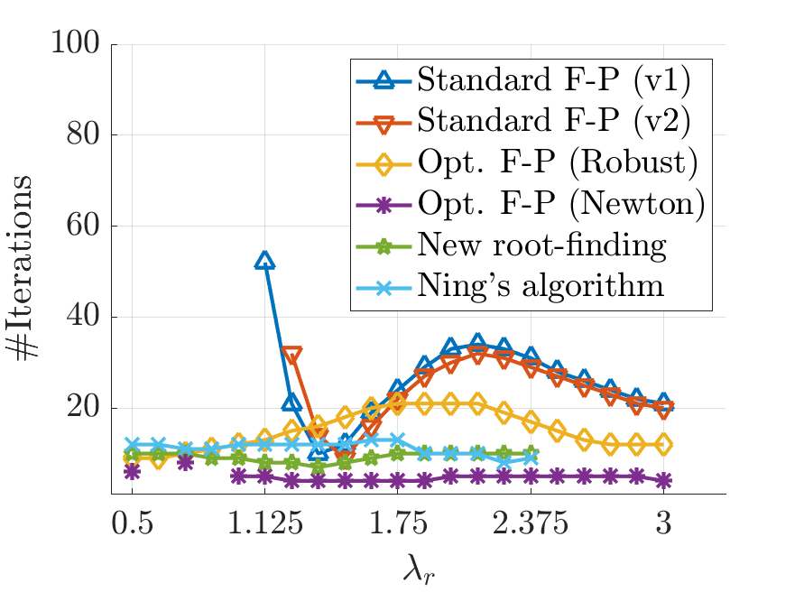
Refer to caption
Refer to caption
Figure 4: Number of iterations required to solve (30) with Algorithm 1 (Standard fixed-point version 1 & 2), Algorithm 2 (Optimized fixed-point, robust and Newton versions) and root-finding approaches (Ning’s algorithm and new root-finding) as function of λr{\lambda_{{\color[rgb]{0,0,0}r}}}. Left: ac=1a_{c}=1, right: ac=1/3a_{c}=1/3. Only convergence cases are reported.

In case of convergence, the obtained limit is the same with all algorithms. We observe that the robust version of Algorithm 2 is the only algorithm that always converges and that its Newton version outperforms all other algorithms and only diverges in three cases.

6.2 Example of a large wind turbine

We consider the IEA Wind 15-MW reference wind turbine22 2 All numerical data related to this example are given in https://github.com/IEAWindTask37.. In this example the blade length is 117 m, decomposed into 5050 elements and designed for a TSR equal to 9. The coefficients CLC_{L} and CDC_{D} take into account 3D-effects by using Du-Selig [16] stall delay 3D correction and are specified for each element. We interpolate them using the Akima algorithm [1, 2] which provides smooth approximations. A full description of the turbine is given in [18].

In our test, we compute optimal parameters (γλrc,cλrc)(\gamma_{\lambda_{{\color[rgb]{0,0,0}r}}}^{c},c_{\lambda_{{\color[rgb]{0,0,0}r}}}^{c}) using the Matlab function fminunc, providing the gradient as in Algorithm 3. For the sake of consistency, with use the same tolerance Tol=10−7=10^{-7} in the stopping criteria of the optimization procedure and of the solution algorithm considered to solve (24), i.e., the algorithms stop when ‖∇Jλr​(γλr,cλr)‖≤\|\nabla J_{\lambda_{{\color[rgb]{0,0,0}r}}}(\gamma_{\lambda_{{\color[rgb]{0,0,0}r}}},c_{\lambda_{{\color[rgb]{0,0,0}r}}})\|\leq Tol and |R​e​s​(φ)|≤|Res(\varphi)|\leq Tol, respectively. For the sake of numerical efficiency, we use a continuation approach, meaning that we optimize the elements sequentially by starting from the blade tip and initialize the optimization of the current element with the design obtained for the element previously considered. This process is itself initialized with optimum approximation applied to the tip element. We then compare it to the actual design, denoted by (γλrt​r​u​e,cλrt​r​u​e)(\gamma_{\lambda_{{\color[rgb]{0,0,0}r}}}^{true},c_{\lambda_{{\color[rgb]{0,0,0}r}}}^{true}) to (γλrc,cλrc)(\gamma_{\lambda_{{\color[rgb]{0,0,0}r}}}^{c},c_{\lambda_{{\color[rgb]{0,0,0}r}}}^{c}). The results are presented in Figure 5, whereas the corresponding values of the power coefficient CPC_{P} are CP​(γλrt​r​u​e,cλrt​r​u​e)=0.4531C_{P}(\gamma_{\lambda_{{\color[rgb]{0,0,0}r}}}^{true},c_{\lambda_{{\color[rgb]{0,0,0}r}}}^{true})=0.453133 3 The actual design is planned to achieve CP=0.489C_{P}=0.489, see [18, p.8], CP​(γλrc,cλrc)=0.4628C_{P}(\gamma_{\lambda_{{\color[rgb]{0,0,0}r}}}^{c},c_{\lambda_{{\color[rgb]{0,0,0}r}}}^{c})=0.4628 and CP​(γλr∗,cλr∗)=0.0127C_{P}(\gamma_{\lambda_{{\color[rgb]{0,0,0}r}}}^{\ast},c_{\lambda_{{\color[rgb]{0,0,0}r}}}^{\ast})=0.0127.

Refer to caption
Refer to caption
Refer to caption
Figure 5: Graphs of γλr∗\gamma_{\lambda_{{\color[rgb]{0,0,0}r}}}^{\ast} and γλrc\gamma_{\lambda_{{\color[rgb]{0,0,0}r}}}^{c}, cλr∗c_{\lambda_{{\color[rgb]{0,0,0}r}}}^{\ast} and cλrcc_{\lambda_{{\color[rgb]{0,0,0}r}}}^{c}, Jλr​(γλr∗,cλr∗)J_{\lambda_{{\color[rgb]{0,0,0}r}}}(\gamma_{\lambda_{{\color[rgb]{0,0,0}r}}}^{\ast},c_{\lambda_{{\color[rgb]{0,0,0}r}}}^{\ast}) and Jλr​(γλrc,cλrc)J_{\lambda_{{\color[rgb]{0,0,0}r}}}(\gamma_{\lambda_{{\color[rgb]{0,0,0}r}}}^{c},c_{\lambda_{{\color[rgb]{0,0,0}r}}}^{c}).

We observe that the optimum approximation gives a very bad design. On the other hand, the optimal design (γλrc,cλrc)(\gamma_{\lambda_{{\color[rgb]{0,0,0}r}}}^{c},c_{\lambda_{{\color[rgb]{0,0,0}r}}}^{c}) appears to be close to the actual design (γλrt​r​u​e,cλrt​r​u​e)(\gamma_{\lambda_{{\color[rgb]{0,0,0}r}}}^{true},c_{\lambda_{{\color[rgb]{0,0,0}r}}}^{true}), except for small values of λr{\lambda_{{\color[rgb]{0,0,0}r}}}, i.e. in the neighborhood of the hub where it only weakly influences the power coefficient. This explains that these two designs give similar values of this coefficient. Remark that the chords cλr∗c_{\lambda_{{\color[rgb]{0,0,0}r}}}^{\ast} and cλrcc_{\lambda_{{\color[rgb]{0,0,0}r}}}^{c} are very large for small values of λr{\lambda_{{\color[rgb]{0,0,0}r}}}, which makes them unrealistic in practice. Though the results do not depend on the considered solution algorithm (up to the tolerance Tol), this one impacts the total number of iterations used to solve (24) required during the optimization process, as shown in Table 3. The robust version and Newton version of Algorithm 2 appear to be the fastest procedures in this example.

Solution algo. Stand. F-P (v1) Stand. F-P (v2) Opt. F-P (robust)
#Iterations 9105 8646 5045
Solution algo. Opt. F-P (Newton) New root-finding Ning’s alg.
#Iterations 1688 5653 5965
Table 3: Number of iterations of the solutions algorithms during the optimization.

7 Conclusion

In this paper, we present a new formulation of the BEM model, which respects the paradigm of this approach in the sense that it decomposes the model into a macroscopic part, related to the momentum theory, and a local part, related to the blade element theory. This framework allows us to obtain existence results and new solution algorithms which outperform the usual algorithms and whose convergence can be analyzed mathematically. We have focused on the case of extracting turbines and a future work could consist in extending our formulation to propellers, which was the initial purpose of this theory. Moreover, some work is required to combine or include this model into modern CFD codes devoted to turbine design. Using BEM model as coarse solver or preconditionner of the fluid-structure interaction system could improve the convergence properties of associated PDE solvers.

Acknowledgments

The authors acknowledge support from ANR Ciné-Para (ANR-15-CE23-0019) and ANR HyFloEFlu (ANR-10-IEED-0006-04). The authors thank the anonymous referees for their insightful suggestions. J.S. thanks Dylan Machado for his careful proofreading of the article.

Appendix: a case of convergence of Algorithm 1 (version 1)

In the case of the simplified model, Algorithm 1 reads as an iterative procedure based on the formula

φk+1:=f~​(φk),\varphi^{k+1}:=\widetilde{f}(\varphi^{k}), (43)

where f~​(x):=π2−atan⁡(λr+μL​(x)​h​(x))\widetilde{f}(x):=\frac{\pi}{2}-{\rm atan}\left({\lambda_{{\color[rgb]{0,0,0}r}}}+\mu_{L}(x)h(x)\right) and h⁡(x):=λr​tan−1⁡x+1sin⁡xh(x):=\dfrac{\lambda_{{\color[rgb]{0,0,0}r}}\tan^{-1}x+1}{\sin x}. This framework makes it possible to obtain bounds for this sequence.

Lemma 15.

Suppose that Assumption 1 holds and that max⁡I+=θλr\max I^{+}=\theta_{\lambda_{{\color[rgb]{0,0,0}r}}}, with μL\mu_{L}{} non-decreasing. If

μL​(θλr)≤μG​(γλr).\mu_{L}(\theta_{\lambda_{{\color[rgb]{0,0,0}r}}})\leq\mu_{G}(\gamma_{\lambda_{{\color[rgb]{0,0,0}r}}}). (44)

and φ0∈[γλr,θλr]\varphi^{0}\in[\gamma_{\lambda_{{\color[rgb]{0,0,0}r}}},\theta_{\lambda_{{\color[rgb]{0,0,0}r}}}], then the sequence defined by (43) satisfies ∀k∈ℕ,φk∈[γλr,θλr]\forall k\in\mathbb{N},\ \varphi^{k}\in[\gamma_{\lambda_{{\color[rgb]{0,0,0}r}}},\theta_{\lambda_{{\color[rgb]{0,0,0}r}}}].

Proof.

Assume that for some k∈ℕk\in\mathbb{N}, φk∈[γλr,θλr]\varphi^{k}\in[\gamma_{\lambda_{{\color[rgb]{0,0,0}r}}},\theta_{\lambda_{{\color[rgb]{0,0,0}r}}}]. Because of (43), we have tan−1⁡φk+1:=λr+μL​(φk)​h​(φk)\tan^{-1}\varphi^{k+1}:={\lambda_{{\color[rgb]{0,0,0}r}}}+\mu_{L}(\varphi^{k})h(\varphi^{k}). Combining it with μL≥0\mu_{L}\geq 0 gives φk+1≤θλr\varphi^{k+1}\leq\theta_{\lambda_{{\color[rgb]{0,0,0}r}}}. Since μL\mu_{L} is increasing and hh is decreasing, tan−1⁡φk+1≤λr+μL​(θλr)​h​(γλr)\tan^{-1}\varphi^{k+1}\leq{\lambda_{{\color[rgb]{0,0,0}r}}}+\mu_{L}(\theta_{\lambda_{{\color[rgb]{0,0,0}r}}})h(\gamma_{\lambda_{{\color[rgb]{0,0,0}r}}}). Because of (44), the latter is bounded by tan−1⁡γλr\tan^{-1}\gamma_{\lambda_{{\color[rgb]{0,0,0}r}}}. The result follows by induction.

We complete this result by a condition about a contraction property.

Lemma 16.

Suppose that μL\mu_{L} is differentiable and denote by μL′\mu_{L}^{\prime} its derivative. The derivative of f~\widetilde{f} satisfies

−sinθλrmaxI+μL′h(γλr)≤f~(φ)′≤sinθλrmaxI+μL|h′(γλr)|.-\sin\theta_{\lambda_{{\color[rgb]{0,0,0}r}}}\max\limits_{I^{+}}\mu_{L}^{\prime}h(\gamma_{\lambda_{{\color[rgb]{0,0,0}r}}})\leq\widetilde{f}{}^{\prime}(\varphi)\leq\sin\theta_{\lambda_{{\color[rgb]{0,0,0}r}}}\max\limits_{I^{+}}\mu_{L}|h^{\prime}(\gamma_{\lambda_{{\color[rgb]{0,0,0}r}}})|.

Proof.

We have f~(φ)′=−11+(λr+μL​(φ)​h​(φ))2(μL′(φ)h(φ)+μL(φ)h′(φ))\widetilde{f}{}^{\prime}(\varphi)=\frac{-1}{1+\left({\lambda_{{\color[rgb]{0,0,0}r}}}+\mu_{L}(\varphi)h(\varphi)\right)^{2}}(\mu_{L}^{\prime}(\varphi)h(\varphi)+\mu_{L}(\varphi)h^{\prime}(\varphi)). Since φ∈(γλr,θλr)\varphi\in(\gamma_{\lambda_{{\color[rgb]{0,0,0}r}}},\theta_{\lambda_{{\color[rgb]{0,0,0}r}}}), μL′​(φ)​h​(φ)≥0\mu_{L}^{\prime}(\varphi)h(\varphi)\geq 0, μL​(φ)​h′​(φ)≤0\mu_{L}(\varphi)h^{\prime}(\varphi)\leq 0, we have −11+(λr+μL​(φ)​h​(φ))2μL′(φ)h(φ)≤f~(φ)′≤−11+(λr+μL​(φ)​h​(φ))2μL(φ)h′(φ)\frac{-1}{1+\left({\lambda_{{\color[rgb]{0,0,0}r}}}+\mu_{L}(\varphi)h(\varphi)\right)^{2}}\mu_{L}^{\prime}(\varphi)h(\varphi)\leq\widetilde{f}{}^{\prime}(\varphi)\leq\frac{-1}{1+\left({\lambda_{{\color[rgb]{0,0,0}r}}}+\mu_{L}(\varphi)h(\varphi)\right)^{2}}\mu_{L}(\varphi)h^{\prime}(\varphi). Because hh and h′h^{\prime} are decreasing on (γλr,θλr)(\gamma_{\lambda_{{\color[rgb]{0,0,0}r}}},\theta_{\lambda_{{\color[rgb]{0,0,0}r}}}), and since μL​(φ)​h​(φ)≥0\mu_{L}(\varphi)h(\varphi)\geq 0, the result follows.

We are now in a position to obtain a conditional convergence result.

Theorem 17.

In addition to the assumptions of Lemma 15, suppose that μL\mu_{L} is differentiable and satisfies

sin⁡θλr​maxI+​μL′​h​(γλr)≤1,sin⁡θλr​maxI+​μL​|h′​(γλr)|≤1.\sin\theta_{\lambda_{{\color[rgb]{0,0,0}r}}}\max\limits_{I^{+}}\mu_{L}^{\prime}h(\gamma_{\lambda_{{\color[rgb]{0,0,0}r}}})\leq 1,\qquad\sin\theta_{\lambda_{{\color[rgb]{0,0,0}r}}}\max\limits_{I^{+}}\mu_{L}|h^{\prime}(\gamma_{\lambda_{{\color[rgb]{0,0,0}r}}})|\leq 1. (45)

Then, if φ0\varphi^{0} belongs to [γλr,θλr][\gamma_{\lambda_{{\color[rgb]{0,0,0}r}}},\theta_{\lambda_{{\color[rgb]{0,0,0}r}}}], the sequence (φk)k∈ℕ(\varphi^{k})_{k\in\mathbb{N}} defined by (43) converges to the unique solution of (24).

Proof.

As a consequence of Lemma 15, the function f~\widetilde{f} maps [γλr,θλr][\gamma_{\lambda_{{\color[rgb]{0,0,0}r}}},\theta_{\lambda_{{\color[rgb]{0,0,0}r}}}] onto itself. From (45) and Lemma 16 we deduce f~\widetilde{f} is contracting. The result follows from the Banach fixed-point theorem.

References

  • [1] H. Akima. A new method of interpolation and smooth curve fitting based on local procedures. Journal of the ACM, 17(4):589–&, 1970.
  • [2] H. Akima. Method of bivariate interpolation and smooth surface fitting based on local procedures. Communications of the ACM, 17(1):18–20, 1974.
  • [3] Y. Bazilevs, M. C. Hsu, I. Akkerman, S. Wright, K. Takizawa, B. Henicke, T. Spielman, and T. E. Tezduyar. 3D simulation of wind turbine rotors at full scale. Part I: Geometry modeling and aerodynamics. Int. J. for Num. Meth. in Fluids, 65(1-3, SI):207–235, 2011.
  • [4] Y. Bazilevs, M. C. Hsu, J. Kiendl, R. Wuechner, and K. U. Bletzinger. 3D simulation of wind turbine rotors at full scale. Part II: Fluid-structure interaction modeling with composite blades. Int. J. Num. Meth. in Fluids, 65(1-3, SI):236–253, 2011.
  • [5] A. Betz. Das maximum der theoretisch möglichen ausnützung des windes durch windmotoren. Zeitschrift für das gesamte Turbinenwesen, 26:307–309, 1920.
  • [6] M. Bossy, J. Espina, J. Moricel, C. Paris, and A. Rousseau. Modeling the wind circulation around mills with a lagrangian stochastic approach. SMAI comp. math., 2:177–214, 2016.
  • [7] E. Branlard. Wind turbine aerodynamics and vorticity-based methods: fundamentals and recent applications. Research topics in wind energy. Springer, 2017.
  • [8] E. Branlard and M. Gaunaa. Superposition of vortex cylinders for steady and unsteady simulation of rotors of finite tip-speed ratio. Wind Energy, 19(7):1307–1323, JUL 2016.
  • [9] R. Brent. Algorithm with guaranteed convergence for finding a zero of a function. Computer Journal, 14(4):422–425, 1971.
  • [10] J. Buhl, M.L. New empirical relationship between thrust coefficient and induction factor for the turbulent windmill state. Technical Report NREL/TP-500-36834, National Renewable Energy Laboratory, Golden, CO, August 2005.
  • [11] T. Burton, D. Sharpe, N. Jenkins, and E. Bossanyi. The Wind Energy Handbook, volume 1. John Wiley and Sons, Ltd, 2001.
  • [12] P. K. Chaviaropoulos and M. O. L. Hansen. Investigating Three-Dimensional and Rotational Effects on Wind Turbine Blades by Means of a Quasi-3D Navier-Stokes Solver . Journal of Fluids Engineering, 122(2):330–336, 02 2000.
  • [13] M. J. Clifton-Smith. Wind turbine blade optimisation with tip loss corrections. Wind Engineering, 33(5):477–496, 2009.
  • [14] M. Drela. XFOIL: An analysis and design system for low Reynolds number airfoils. In T. J. Mueller, editor, Low Reynolds Number Aerodynamics, pages 1–12. Springer, 1989.
  • [15] L. Du, G. Ingram, and R. G. Dominy. A review of H-Darrieus wind turbine aerodynamic research. Proc. Inst. of Mech. Eng., Mech. Eng. Sci. (C), 233(23-24, SI):7590–7616, 2019.
  • [16] Z. Du and M. Selig. A 3-d stall-delay model for horizontal axis wind turbine performance prediction. In 1998 ASME Wind Energy Symposium, 1998.
  • [17] D. Eggleston and F. Stoddard. Wind turbine engineering design. Springer, New-York, 1987.
  • [18] G. Evan, J. Rinker, L. Sethuraman, F. Zahle, B. Anderson, G. Barter, N. Abbas, F. Meng, P. Bortolotti, W. Skrzypinski, G. Scott, R. Feil, H. Bredmose, K. Dykes, M. Shields, C. Allen, and A. Viselli. Definition of the iea 15-megawatt offshore reference wind. Technical Report NREL/TP-5000-75698, National Renewable Energy Laboratory, Golden, CO, March 2020.
  • [19] W. Froude. On the elementary relation between pitch, slip and propulsive efficiency. Trans. Roy. Inst. Naval Arch., 19(47):47–57, 1878.
  • [20] H. Glauert. The analysis of experimental results in the windmill brake and vortex ring states of an airscrew. London: Aeronautical Research Committee, 1026, 1926.
  • [21] H. Glauert. Airplane propellers. In W. F. Durand, editor, Aerodynamic Theory, volume 4, pages 169–360. Berlin: Julius Springer, 1935.
  • [22] H. Glauert. The Elements of Aerofoil and Airscrew Theory. Cambridge University Press, 1983.
  • [23] M. O. Hansen. Aerodynamics of Wind Turbines. Taylor and Francis, 2015.
  • [24] M.-C. Hsu and Y. Bazilevs. Fluid-structure interaction modeling of wind turbines: simulating the full machine. Comp. Mech., 50(6, SI):821–833, 2012.
  • [25] N. Joukowsky. Vortex theory of screw propeller, i. Trudy Otdeleniya Fizicheskikh Nauk Obshchestva Lubitelei Estestvoznaniya, 16(1):1–31, 1912.
  • [26] N. Joukowsky. Windmill of the NEJ type. Trans. of Cent. Inst. for Aero-Hydrodyn., 1920.
  • [27] N. Joukowsky. Joukowsky NE. Collected papers, volume VI. The Joukowsky Institute for AeroHydrodynamics, Moscow-Leningrad, Russia: ONTI, 1937.
  • [28] F. Lanchester. A contribution to the theory of propulsion and the screw propeller. Trans. Inst. of Naval Arch., 57:98–116, 1915.
  • [29] C. Lock, H. Bateman, and H. Townend. An extension of the vortex theory of airscrews with applications to airscrews of small pitch, including experimental results. A.R.C. Research Reports and Memoranda, 1014, 1925.
  • [30] H. A. Madsen, T. J. Larsen, G. R. Pirrung, A. Li, and F. Zahle. Implementation of the blade element momentum model on a polar grid and its aeroelastic load impact. Wind Energy Science, 5(1):1–27, JAN 2 2020.
  • [31] D. Maniaci. 49th AIAA Aerospace Sciences Meeting including the New Horizons Forum and Aerospace Exposition, chapter An Investigation of WT_Perf Convergence Issues. Aerospace Sci. Meetings. American Institute of Aeronautics and Astronautics, 2011.
  • [32] J. Manwell, J. Mcgowan, and A. L Rogers. Wind Energy Explained: Theory, Design and Application, Second Edition, volume 30. John Wiley and Sons, Ltd, 2006.
  • [33] M. McWilliam and C. Crawford. The behavior of fixed point iteration and newton-raphson methods in solving the blade element momentum equations. Wind Engineering, 35(1):17–31, 2011.
  • [34] A. Ning, G. Hayman, R. Damiani, and J. M. Jonkman. Development and validation of a new blade element momentum skewed-wake model within aerodyn. In Proc. of the 33rd Wind Energy Symp., 2015.
  • [35] S. A. Ning. A simple solution method for the blade element momentum equations with guaranteed convergence. Wind Energy, 17(9):1327–1345, SEP 2014.
  • [36] V. L. Okulov, J. N. Sorensen, and D. H. Wood. The rotor theories by Professor Joukowsky: Vortex theories. Progress In Aerospace Sciences, 73(SI):19–46, FEB 2015.
  • [37] V. L. Okulov and G. A. M. van Kuik. The Betz-Joukowsky limit: on the contribution to rotor aerodynamics by the British, German and Russian scientific schools. Wind Energy, 15(2):335–344, MAR 2012.
  • [38] B. A. Prandtl L. Vier abhandlungen zur hydrodynamik und aerodynamik. Göttinger Klassiker der Strömungsmechanik, 3:1–100, 2010. (Flüssigkeit mit kleiner Reibung; Tragflügeltheorie, I. und II. Mitteilung; Schraubenpropeller mit geringstem Energieverlust).
  • [39] W. J. M. Rankine. On the mechanical principles of the action of propellers. Trans. Roy. Inst. Naval Arch., 6:13–30, 1865.
  • [40] A. P. Schaffarczyk. Introduction to wind turbine aerodynamics. Green Energy and Technology. Springer, 2014.
  • [41] W. Shen, R. Mikkelsen, J. Sørensen, and C. Bak. Tip loss corrections for wind research turbine computations. Wind Energy, 8(4):457–475, 2005.
  • [42] H. Snel, R. Houwink, G. van Bussel, and A. Bruining. Sectional prediction of 3d effects for stalled flow on rotating blades and comparison with measurements. In Proceedings of European Community Wind Energy Conference, pages 395–399, 1993.
  • [43] Q. Song and W. D. Lubitz. Bem simulation and performance analysis of a small wind turbine rotor. Wind Eng., 37(4):381–399, 2013.
  • [44] J. Sørensen. Aerodynamic Aspects of Wind Energy Conversion. In Davis, SH and Moin, P, editor, Annual Review Of Fluid Mechanics, volume 43 of Annual Review of Fluid Mechanics, pages 427–448. Annual Reviews, 2011.
  • [45] J. Sørensen. General Momentum Theory for Horizontal Axis Wind Turbines. Springer, 2016.
  • [46] D. Spera, editor. Wind Turbine Technology: Fundamental Concepts in Wind Turbine Engineering, Second Edition. ASME, New York, NY, 2009.
  • [47] Z. Sun, W. Z. Shen, J. Chen, and W. J. Zhu. Improved fixed point iterative method for blade element momentum computations. Wind Energy, 20(9):1585–1600, SEP 2017.
  • [48] G. van Kuik. The Fluid Dynamic Basis for Actuator Disc and Rotor Theories. Amsterdam: IOS Press, 2018.
  • [49] G. A. M. van Kuik. The Lanchester-Betz-Joukowsky limit. Wind Energy, 10(3):289–291, 2007.
  • [50] G. A. M. van Kuik, J. N. Sorensen, and V. L. Okulov. Rotor theories by Professor Joukowsky: Momentum theories. Progress In Aerospace Sciences, 73(SI):1–18, FEB 2015.
  • [51] K. W. Van Treuren. Small-Scale Wind Turbine Testing in Wind Tunnels Under Low Reynolds Number Conditions. Journal of Energy Resources Technology, 137(5), 09 2015. 051208.
  • [52] R. E. Wilson, P. B. S. Lissaman, and S. N. Walker. Aerodynamic performance of wind turbines. final report. ERDA/NSF/04014-76/1, 1976.
  • [53] D. H. Wood. Application of extended vortex theory for blade element analysis of horizontal-axis wind turbines. Renewable Energy, 121:188–194, JUN 2018.