Deep Learning of Chaos ClassificationPreprint: AIP/123-QED

Woo Seok Lee Affiliation: Center for Theoretical Physics of Complex Systems, Institute for Basic Science, 34051 Daejeon, Korea Sergej Flach Affiliation: Center for Theoretical Physics of Complex Systems, Institute for Basic Science, 34051 Daejeon, Korea Affiliation: Basic Science Program, Korea University of Science and Technology (UST), 34113 Daejeon, Korea

August 11, 2026

Abstract

We train an artificial neural network which distinguishes chaotic and regular dynamics of the two-dimensional Chirikov standard map. We use finite length trajectories and compare the performance with traditional numerical methods which need to evaluate the Lyapunov exponent. The neural network has superior performance for short periods with length down to 10 Lyapunov times on which the traditional Lyapunov exponent computation is far from converging. We show the robustness of the neural network to varying control parameters, in particular we train with one set of control parameters, and successfully test in a complementary set. Furthermore, we use the neural network to successfully test the dynamics of discrete maps in different dimensions, e.g. the one-dimensional logistic map and a three-dimensional discrete version of the Lorenz system. Our results demonstrate that a convolutional neural network can be used as an excellent chaos indicator.

In low-dimensional dynamical systems with a mixed phase space, both regular and chaotic domains coexist. Lyapunov exponents characterise the time-averaged exponential divergence of nearby orbits in phase space, and are traditional chaos indicators telling regular (zero exponent) from chaotic (nonzero exponent) dynamics apart. In computational approaches, Lyapunov exponents are calculated through long time iterations as finite time averages of properly defined observables. To tell whether an orbit is regular and chaotic means to tell whether the finite time average tends to zero or nonzero values in the infinite time limit. Such traditional methods therefore suffer from notorious uncertainties and need iteration times which are orders of magnitude longer than typical Lyapunov times (the inverse of the exponents). On the other side deep learning algorithms turned to be useful to train networks which then serve as efficient classifiers. These can be used to study heartbeat irregularities, weather forecasting, complex dynamics reconstruction, pattern recognition and feature extraction, among many others. When using in particular a convolutional neural network, the present work shows that a novel classifier emerges, which operates at high accuracy yet uses finite time orbits which are orders of magnitude shorter than the ones needed for the same accuracy with traditional Lyapunov methods.

I Introduction

Chaotic dynamics exists in many natural systems, such as heartbeat irregularities, weather and climate Skinner et al. 1990; Slingo and Palmer 2011. Such dynamics can be studied through the analysis of proper mathematical models which generate nonlinear dynamics and determenistic chaos. Chaotic and regular dynamics can co-exist in the phase space of low-dimensional systems Ott 2002. To distinguish chaotic from regular dynamics, the tangent dynamics is used to compute Lyapunov exponents $\lambda$ . In practice one integrates the tangent dynamics along a given trajectory and averages a finite time Lyapunov exponent $\lambda(t)$ . The averaging time $T$ needed to reliably tell regular ( $\lambda=0$ ) from chaotic ( $\lambda\neq 0$ ) trajectories apart is usually orders of magnitude larger than the Lyapunov time $T_{\lambda}\equiv 1/\lambda$ .

Here, we introduce a machine learning approach that alleviates the problems of calculating Lyapunov exponents and can be used as a new chaos indicator. Machine learning has shown tremendous performance e.g. in pattern recognition Dodge and Karam 2017; Al-Saffar, Tao, and Talab 2017. Machine learning approaches turned useful to solve partial differential equations and identify hidden physics models from experimental data Rudy et al. 2017; Han, Jentzen, and E 2018; Raissi and Karniadakis 2018. Machine learning was used recently to predict future chaotic dynamics details from time series data without knowledge of the generating equations Agrawal et al. 2019; Pathak et al. 2018. In this paper, we introduce a machine learning way to use short time series data for telling chaos from regularity apart. We train a neural network using chaotic and regular trajecories from the Chirikov standard map. Our method has a success rate of 98% using trajectories with length $10T_{\lambda}$ , while conventional methods need up to $10^{4}T_{\lambda}$ to reach the same accuracy. The main reason for the small but finite failure rate of our machine learning method is due to sticky orbits. These orbits are chaotic,yet can mimic regular ones for long times due to trapping in fractal boundary phase space regions separating chaotic and regular dynamics. Our method is also surprisingly successfull when trained with Standard Map data but tested on maps with different dimensions such as the logistic map ( $d=1$ ) and the Lorenz system ( $d=3$ ).

II The Chirikov Standard Map

The Chirikov standard map is an area-preserving map in dimension $d=2$ Lichtenberg and Lieberman 2013 also known as the kicked rotor Ott 2002 :

	$\displaystyle p_{n+1}=p_{n}+\frac{K}{2\pi}sin(2\pi x_{n})\qquad mod\ 1\;,$		(1)
	$\displaystyle x_{n+1}=x_{n}+p_{n+1}\qquad mod\ 1\;.$		(1)

The kick strength $K$ controls the degree of nonintegrability and chaos appearing in the dynamics generated by the map.

Refer to caption — Figure 1: Examples of Poincare sections of the standard map. (a) K=0.5, (b) K=1.0, (c) K=2.0, (d) K=2.5.

Consider the case when $K=0$ . Eq. 1 reduces to $p_{n+1}=p_{n}\quad(mod\ 1)$ and $x_{n+1}=x_{n}+p_{n+1}\quad(mod\ 1)$ which is integrable and every orbit resides on an invariant torus. The orbit can exhibit periodic or quasi-periodic behavior depending on the initial conditions ( $p_{0},x_{0}$ ). For small values of $K$ e.g. $K=0.5$ (Fig.1(a)) most of these orbits persist, with tiny regions of chaotic dynamics appearing which are not visible on the presented plotting scales. At $K=K_{c}\approx 0.97$ the last invariant KAM tori are destroyed and a simply connected chaotic sea is formed which allows for unbounded momentum diffusion. For larger values of $K$ the chaotic fraction grows confining regular dynamics to regular islands embedded in a chaotic sea (Fig. 1). Further increase of $K$ leads to a flooding of the regular islands by the chaotic sea.

III Lyapunov exponents and predictions

The Lyapunov exponent (LE) characterizes the exponential rate of separation of a trajectory $\{p_{n},x_{n}\}$ and its infinitesimal perturbation $\{\delta_{n},\zeta_{n}\}$ :

	$\displaystyle p_{n+1}+\delta_{n+1}$	$\displaystyle=(p_{n}+\delta_{n})+\frac{k}{2\pi}sin(2\pi(x_{n}+\zeta_{n}))$		(2)
	$\displaystyle x_{n+1}+\zeta_{n+1}$	$\displaystyle=(x_{n}+\zeta_{n})+(p_{n+1}+\delta_{n+1})$		(2)

Linearizing (2) in the perturbation yields the tangent dynamics generated by the variational equations

	$\displaystyle\delta_{n+1}$	$\displaystyle=\delta_{n}+k\zeta_{n}cos(2\pi x_{n})$		(3)
	$\displaystyle\zeta_{n+1}$	$\displaystyle=\zeta_{n}+\delta_{n+1}$		(3)

For computational pruposes $\delta$ and $\zeta$ can be rescaled after any time step without loss of generality, while keeping the rescaling factor. The LE $\lambda$ for each trajectory is obtained from the time dependence of $\lambda_{N}$ :

\lambda_{N}=\frac{1}{N}\sum_{n=2}^{N}\ln(\frac{\sqrt{\delta_{n}^{2}+\zeta_{n}^{2}}}{\sqrt{\delta_{n-1}^{2}+\zeta_{n-1}^{2}}})\;,\;\lambda=\lim_{N\rightarrow\infty}\lambda_{N}\;.

(4)

The Lyapunov time is then defined as $T_{\lambda}\equiv 1/\lambda$ . For the main chaotic sea it is a function of the control parameter $K$ . A suitable fitting function yields $\lambda\approx\ln(0.7+0.42K)$ Harsoula, Karamanos, and Contopoulos 2019.

For a regular trajectory $\lambda_{N}\sim 1/N$ and $\lambda=0$ , at variance to a chaotic trajectory for which $\lambda_{N}$ saturates at $\lambda$ at a time $N\approx T_{\lambda}$ . Technically this saturation, and the value of $\lambda$ can be safely confirmed and read off only on time scales $N\approx 10^{2}..10^{3}T_{\lambda}$ , without becoming a quantifiable distinguisher of the two types of trajectories, see Fig.2.

Figure 2:

\lambda_{N}

versus

N

for a chaotic (triangles) respectively regular (squares) trajectory with

K=1.0

. The dashed horizontal line indicates the value of

\lambda

for the chaotic trajectory, and the dashed vertical one the corresponding value of

T_{\lambda}

To quantify our statements, we run the standard map at $K=2.5$ Fig.1(d). We use a grid of $51\times 51$ points which partitions the phase space $\{p,x\}$ into a square lattice. We use the corresponding 2601 initial conditions and generate trajectories. Each trajectory returns a function $\lambda_{N}$ . We plot the resulting histogram for $N=20$ and $N=3\cdot 10^{5}$ in Fig.3 (a) and (b) respectively. For $N\rightarrow\infty$ the histogram should show two bars only - one at $\lambda_{N}=0$ (all regular trajectories) and one at $\lambda_{N}=\lambda$ (all chaotic trajectories). For finite $N$ the distributions smoothen. Note that even negative values $\lambda_{N}$ are generated due to fluctuations and finite averaging times. To tell chaotic from regular dynamics apart, we use the following protocol. We identify the two largest peaks in each histogram, and identify the threshold dividing dynamics into regular and chaotic as the deepest minimum between them (in case of a degeneracy, the one with the smallest value of $\lambda_{N}$ ). The location of the threshold is shown for $N=20$ and $N=3\cdot 10^{5}$ in Fig.3 (a) and (b) respectively. We then assign a chaos respectively regular label to each trajectory. This label can fluctuate as a function of time for any given trajectory. We use the division for the largest simulation time $N=3\cdot 10^{5}$ as a reference (’true’) label for all trajectories. The success rate in predicting the correct regular $P_{R}$ or chaotic $P_{C}$ label is defined by the ratio of the correctly predicted labels within each subgroup of identical true labels. Likewise the success rate of predicting any label correctly is denoted by $P_{tot}$ . The results are plotted versus time $N$ in Fig.3 (c). While regular labels are predicted with high accuracy, chaotic ones are reaching 98 $\%$ at only $N\approx 10^{3}T_{\lambda}$ . The low success rate $P_{C}$ is therefore also lowering the total success rate $P_{tot}$ .

IV Neural networks and predictions

The input data of an artificial neural network consisting of only fully connected layers are limited to a one-dimensional (array) form Ramsundar and Zadeh 2018. Fully connected layers connect all the inputs from one layer to every activation unit of the next layer. The standard map generates sequences embedded in two dimensions. In order to learn data embedded in dimensions two or larger, the data must be flattened, and spatial information can get lost. A Convolutional Neural Network (CNN) is known to learn while maintaining spatial informations of images LeCun et al. 1999. A CNN is usually configured with convolution and pooling layers. The former employ convolutional integrals with input data and filters to produce output feature maps. An additional activation function turns the network non-linear. At the end of the convolution layers a pooling layer is added which performs value extraction in a given pooling region. Through multiple convolution layers and pooling layers, the network can improve its prediction features. Finally, a fully connected layer generates classified output data. For binary classification, the last layer consists of one node. Its output value is either zero or one. We refer the reader to Appendix A for further technical details of the CNN we use.

IV.1 The standard map

The input of the neural network is a time series $(p_{n},x_{n})$ from Eq. 1. The trajectory $(p_{n},x_{n})$ shows regular or chaotic behavior depending on the initial values $(p_{0},x_{0})$ . Each of the trajectories is assigned a class label based on the Lyapunov time: Class $R$ corresponds to a non-chaotic trajectories while $C$ corresponds to a chaotic trajectories. We remind that the phase space is discretized into $51\times 51=2601$ grid points. The training and testing is quantified with a set of parameters: i) $K_{min}$ and $K_{max}$ denote the range of training values of $K$ on an equidistant grid with $M_{K}$ values; ii) $M_{tr}$ is the number of training trajectories per $K$ value; iii) $N_{K}$ is the training trajectory length; iv) $M_{tt}$ is the number of test trajectories per $K$ value.

To quantify the CNN performance, we assign a discrete label to each of the initial phase space points - $C$ respectively $R$ based on the Lyapunov exponent method with trajectory length $N=3\cdot 10^{5}$ . This way we separate all phase space points into two sets - $C$ and $R$ , each containing $A_{C}$ and $A_{R}$ points. We then run the CNN prediction on trajectories of length $N=20$ which start from each of the gridded phase space points. We compute the accuracy quantifying probabilities

P_{C}=\frac{B_{C}}{A_{C}},~P_{R}=\frac{B_{R}}{A_{R}},~P_{tot}=\frac{B_{C}+B_{R}}{A_{C}+A_{R}}

(5)

where $B_{C}$ and $B_{R}$ are the numbers of trajectories predicted by the CNN to be chaotic respectively regular within each of the true sets $A_{C}$ and $A_{R}$ . Thus strictly $B_{C}\leq A_{C}$ and $B_{R}\leq A_{R}$ .

Fig. 3(d) compares the CNN performance to the standard Lyapunov base one. Accuracies of 98% and more are reached by the CNN for trajectory length $N_{K}\geq 30$ . Similar accuracies need trajectory length $N\approx 10^{4}$ and more when using standard Lyapunov testing. Fig.4 shows the CNN performance with $N_{K}=10$ in the phase space of the standard map. We observe that most of the failures correspond to chaotic trajectories starting in the fractal border region close to regular islands. These trajectories can be trapped for long times in the border region, with trapping time distributions exhibiting power law tails Zaslavsky 1998.

To quantify the performance of the CNN, we first vary the $N_{K}$ from 1 to 20 (Table 1). The network is trained with chaotic and regular trajectories for $K_{min}=1.0$ , $K_{max}=2.0$ , $M_{K}=11$ , and $1\leq N_{K}\leq 20$ and the network performance is evaluated for $3\leq K\leq 3.5$ and $M_{K}=6$ . The CNN requires that the length of test trajectories is always kept equal to the length of the training trajectories. Note that the Lyapunov time $T_{\lambda}\approx 2$ for the test values of $K$ . The CNN shows improvement of the accuracy with increasing $N_{K}$ . While the performance fluctuates with varying $K$ , it shows excellent results for $N_{K}$ values and clearly outperforms the Lyapunov exponent based method.

	$20$	$18$	$16$	$14$	$12$	$10$	$2$	$1$
	$P_{C}$ / $P_{R}$	$P_{C}$ / $P_{R}$	$P_{C}$ / $P_{R}$	$P_{C}$ / $P_{R}$	$P_{C}$ / $P_{R}$	$P_{C}$ / $P_{R}$	$P_{C}$ / $P_{R}$	$P_{C}$ / $P_{R}$
3.0	0.99/0.99	0.93/0.98	0.95/0.98	0.92/0.98	0.97/0.96	0.83/0.95	0.89/0.97	0.78/1.0
3.1	0.90/0.98	0.94/0.96	0.96/0.96	0.93/0.96	0.90/0.96	0.83/0.91	0.90/0.93	0.79/1.0
3.2	0.93/0.95	0.94/0.97	0.96/0.97	0.93/0.97	0.97/0.94	0.85/0.91	0.90/0.92	0.79/1.0
3.3	0.97/0.99	0.93/0.99	0.95/0.99	0.93/0.99	0.94/0.96	0.85/0.93	0.89/0.98	0.77/1.0
3.4	0.94/0.99	0.89/0.97	0.94/0.96	0.92/0.98	0.93/0.97	0.82/0.93	0.88/0.98	0.76/1.0
3.5	0.93/0.94	0.93/0.93	0.96/0.88	0.92/0.99	0.92/0.91	0.83/0.92	0.87/0.94	0.76/1.0

Table 1: CNN performance. For each K value, 2601 different initial values (

p_{0,i},x_{0,j}

) were selected as (

p_{0,i}=(i-1)\frac{1}{50},x_{0,j}=(j-1)\frac{1}{50},~(i,j\in\mathbb{Z},\>1\leq i,j\leq 51,\;)

). Other parameters are listed in the main text.

We then further test the CNN performance for untrained $K$ values by varying the training $K$ range and other relevant training parameters in Fig. 5. The network shows better performance on untrained K values when trained with a set of different K values. As expected, smaller numbers of training $K$ values yield poorer accuracy due to overtraining. With increasing training range of $K$ values and ranges the network improves its chaos region predictions for untrained K values.

IV.2 Training with the standard map, testing the logistic map

We proceed with testing how the CNN trained with standard map data performs in predicting chaos for other maps. We choose the logistic map as a simple one-dimensional chaotic test bed. The logistic map is written as $x_{n+1}=rx_{n}(1-x_{n})$ . The parameter $r$ controls the crossover from regular to chaotic dynamics, which happens at $r_{c}\approx 3.56995$ . We use two training methods. The first one trains the network only with the $p_{n}$ data sequence from the standard map in Eq. 1. We coin that trained network 1D. The second one is the original CNN discussed above, coined here 2D. As shown in Fig. 6, the network mainly generates errors at the boundary of chaos region similar to the standard map. For $2.5\leq r\leq 4.0$ the accuracy is 84 $\%$ for 2D network and 90% for the 1D network.

IV.3 Training with the standard map, testing the Lorenz system

Next we test Lorenz system which is a three-dimensional map, with a CNN trained on the two-dimensional standard map. The Lorenz system is given by the following map equations:

	$\displaystyle X_{n+1}=X_{n}+\sigma\Delta(Y_{n}-X_{n}),$		(6)
	$\displaystyle Y_{n+1}=Y_{n}+\rho\Delta X_{n}-\Delta X_{n}Z_{n}-\Delta Z_{n},$
	$\displaystyle Z_{n+1}=z_{n}+\Delta X_{n}Y_{n}-\beta\Delta Z_{n}.$

The parameters $\sigma=10$ , $\beta=\frac{8}{3}$ , and $\Delta n=0.001$ . The chaos parameter $0\leq\rho\leq 39.8$ was varied in steps of 0.2. Because the network is trained with 2D data (standard map), the prediction is performed by selecting only two dimensions in the 3D Lorenz system ( $(X_{n},Y_{n}),(X_{n},Z_{n}),(Y_{n},Z_{n})$ ). As Fig. 7 (a) shows, using trajectories obtained from Eq. 6 directly as a network input classifies most of them as chaotic. We think this happens because the trajectory data of the standard map used for training are bounded between 0 and 1, but the trajectories from Lorenz system are not. Input values that exceed these boundaries cause nodes in the network to be active regardless of the input characteristics. Therefore we normalize the input data from the Lorenz system. This leads to a drastic increase of accuracy as shown in Fig. 7 (b). We also tested the outcome when selecting only one dimension in the Lorenz system for the input vector. We find a strong reduction of the accuracy. We therefore conclude that the training and testing data are yielding best performance when for both the minimum of the two dimensions (training map, testing map) is chosen.

V Conclusion

We trained convolutional neural networks with time series data from the two-dimensional standard map. As a result, the network can classify unknown short trajectory sequences into chaotic or regular with high accuracy. To reach accuracies of up to 98% we need trajectory segments with length less than 5-10 Lyapunov times. Similar accuracies need 100-1000 longer segments when using traditional classifiers based on measuring Lyapunov exponents. The main cause of errors is due to fractal phase space structures at the boundaries between chaotic and regular dynamics. Trajectories launched in these regions yield sticky trajectories which can mimick regular ones for long times, only to escape at even larger times into the chaotic sea. We also used a network trained with two-dimensional standard map data to classify chaotic and regular dynamics in one- and three-dimensional maps. Surprisingly high accuracy is reached when the training data are projected into one dimension for predictions on the one-dimensional logistic map, and when to-be-predicted data from the three-dimensional Lorenz system are projected onto two dimensions. We conclude that accuracy is optimized when the minimum of the two dimensions (training map, testing map) is chosen for both training and testing.

Acknowledgements.

This work was supported by the Institute for Basic Science, Project Code IBS-R024-D1. SF thanks Konstantin Kladko for discussions during a visit to IBS, which led to the main idea of machine learning based chaos testing, and Natalia Khotkevych for early attempts to figure a realization pathway.

Appendix A Details of the neural network structure

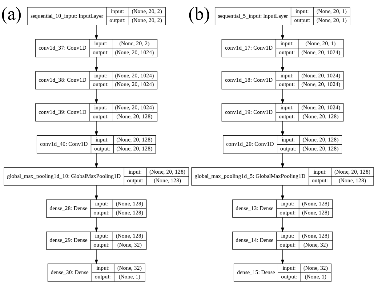
The neural network model we use to analyze the chaotic pattern is the convolutional neural network (CNN) LeCun et al. 1999 with a fully connected (FC) network Krizhevsky, Sutskever, and Hinton 2012; Goodfellow, Bengio, and Courville 2016. The required nonlinear response of the system is provided by the rectified linear unit (ReLU) Nair and Hinton 2010; Goodfellow, Bengio, and Courville 2016. For supervised learning, we use a cross entropy as loss function Goodfellow, Bengio, and Courville 2016. Fig. 8 shows one of the CNN structures used here. In the figure, 1024 filters in the first layer scan the input data independently, then yield 1024 feature maps which are used as the input data for the second layer after applying the activation function ReLU. After processing through all convolutional layers, we rearranged the pixels of the last feature maps into one-dimensional data for the fully connected layers. In the last layer we set the desired output: 1 is a chaotic, and 0 is a regular trajectory.

We use a two-dimensional convolutional filter. The data comprise multiple spatial channels and each channel gives time-series data. The relation between the 2D input vector $a$ and the convolution layer output vector $z$ is

z^{(\ell)}_{i,j,m}=\sum^{F_{row}}_{q=1}\sum^{F_{col}}_{p=1}w^{(\ell)}_{p,q,m}a^{(\ell-1)}_{(i+p-1),(j+q-1)}+b^{(1)}_{m}.

(7)

After calculating $z$ , the nonlinear activation function (We used ReLU) is used to obtain the value of $a$ of the next layer:

a^{(\ell)}_{i,j,m}=\textrm{ReLU}(z^{(\ell)}_{i,j,m}),

(8)

where $i,j$ are input element indices, $p,q$ are filter element indices, $m$ is the filter index (e.g. m = 1024 means that 1024 filters of size $F_{row}\times F_{col}$ were used), and $\ell$ is the layer index (the indices of input and first layer are $\ell$ = 0 and $\ell$ = 1 respectively). The weight $w^{(\ell)}_{p,q,m}$ is the $(p,q)^{th}$ element of $m^{th}$ filter. The bias $b_{m}$ is a constant. The filter size is $F_{row}\times F_{col}$ , where we chose $F_{row}=2$ and $F_{col}=1$ . To apply the filter to all the elements of the input, the boundary is filled with zeroes to match the size of the input, which is called zero padding Dumoulin and Visin 2016. The 2D input through the convolution layer has a dimension of $(i,j,m)$ due to the number of filters $m$ in the convolution layer. Accordingly, the input / output relationship of the next layer is as follows:

z^{(\ell)}_{i,j,n}=\sum^{M_{\ell}}_{n=1}\sum^{F_{row}}_{q=1}\sum^{F_{col}}_{p=1}w^{(\ell)}_{p,q,n}a^{(\ell-1)}_{(i+p-1),(j+q-1),m}+b^{(\ell)}_{n},

(9)

where $M_{\ell}$ is the number of filters between the $\ell^{th}$ and $(\ell-1)^{th}$ layers, $\ell$ has a range of 1 to $L$ . After convolution, it processes through the activation function as shown in Eq. 8.

As shown in Fig. 8, there is a pooling layer at the end of the convolution layers. This flattens the convolutional output by finding the maximum according to the filter dimension of the input (Eq. 10).

a^{(\ell)}_{m}=max(a^{(\ell)}_{i,j,m}).

(10)

The reason for flattening the output is to use the convolutional output as the input of the fully connected layer:

z^{(\ell)}_{i}=\sum^{K}_{j=1}w^{(\ell-1)}_{j,i}a^{(\ell-1)}_{j},

(11)

where $w_{i,j}$ is a weighted connection between the $j^{th}$ component of $(\ell-1)^{th}$ layer and the $i^{th}$ component of $(\ell)^{th}$ layer and $K$ is the number of nodes in the $(\ell-1)^{th}$ layer. As in Eq. 12, the activation function uses ReLU:

a^{(\ell)}_{i}=\textrm{ReLU}(z^{(\ell)}_{i}).

(12)

The output value of the network, when obtained in this way, is different from the desired output because it is obtained from the unfitted $w$ value. $w$ updates in the direction of reducing this difference and we call this difference the loss or cost. In this work, we selected the cross entropy as the loss function, defined as

C=-\sum_{k=1}^{N_{L}}{(a^{true}_{k}log(a^{(L)}_{k})+(1-a^{true}_{k})log(1-a^{(L)}_{k}))},

(13)

where $N_{L}$ is the number of nodes in the output layer and $a^{true}_{k}$ is the desired output at the $k^{th}$ node. The cross-entropy loss function can reflect the degree of error to weight updates better than the mean square error loss function (MSE, MSE $=\frac{1}{N_{L}}\sum_{k=1}^{N_{L}}(a^{true}_{k}-a^{(L)}_{k})^{2}$ ) because of the log term and is known as a cost function suitable for classification problems Nielsen 2015. Similar to the energy minimization problem in physics, supervised learning minimizes a cost function $C$ at the output layer.

Training the neural network means finding optimized parameters $w^{(\ell)}_{pqm}$ and $b_{n}^{(l)}$ that minimize $C$ . We use an Adaptive Moment Estimation (Adam) algorithm for the optimization of learning Kingma and Ba 2015. As far as we know, the choice of optimization algorithm has little impact on the network performance, but is instead mainly related to the speed of learning. It is known that an Adam algorithm can find fitting variables faster than stochastic gradient descent methods, RMS prop and AdaDelta Kingma and Ba 2015.

Appendix B Network comparison

In this section, we compare three different network architectures. First, we consider a fully connected neural network (FCN) and then compare it to other machine learning methods. The FCN is chosen because it is the most basic structure of deep learning classifiers. We also consider a recurrent neural network (RNN) Sherstinsky 2020. The RNNs are usually used to deal with temporal dynamic behavior.

We consider supervised classification with labels indicating chaos or regularity, where the input of the neural networks is fixed at $N_{K}=20$ , and the output is one node for the corresponding label for training. The neural networks presented in this paper end with a sigmoid layer.

The first type of network considered in this section is a fully connected network, which consists of multiple fully connected layers and each layer has a nonlinear activation function. We use eight hidden layers with ReLU (Rectified Linear Unit) activation and the number of hidden neurons in each layer is [256, 256, 512, 512, 512, 256, 128, 64]. The network is trained with the Adaptive Moment Estimation (Adam) algorithm Kingma and Ba 2015.

Recurrent neural networks (RNN) are neural networks for processing sequential data. RNN uses the current input as well as any previously processed input. This is possible with a loop structure between the RNN input and the output. Each node in a given layer is connected with a directed connection to the current layer. Because of this, the RNN is expected to have a function of memory. The sequence itself has information, and recurrent networks use this information through the loop structure. We use three type of RNNs: simpleRNN Sherstinsky 2020, LSTM Sherstinsky 2020; Gers, Schmidhuber, and Cummins 1999, and GRU Cho et al. 2014. Three RNN cells(layers) were used, each with 200 hidden neurons. After the RNN cells, three fully connected layers are connected with the size of 200, 100 and 32 respectively.

Classifiers	$P_{tot}$	$P_{C}$	$P_{R}$
FCN	0.89	0.88	0.91
SimpleRNN	0.94	0.96	0.92
GRU	0.95	0.96	0.93
LSTM	0.94	0.96	0.93
CNN	0.96	0.94	0.97

Table 2: Performance for different deep learning classifiers. The networks are trained with chaotic and regular trajectories for

K_{min}=1.0,\;K_{max}=2.0,\;M_{K}=11,\;M_{tr}=2601

and

N_{K}=20

. The network performances are evaluated for

K_{min}=3.0,\;K_{max}=3.5,\;M_{K}=6,\;M_{tt}=2601

and

N_{K}=20

. For each K value, 2601 different initial values (

p_{0,i},x_{0,j}

) were selected as (

p_{0,i}=(i-1)\frac{1}{50},x_{0,j}=(j-1)\frac{1}{50},~(i,j\in\mathbb{Z},\>1\leq i,j\leq 51,\;)

It is known that recurrent networks perform well for sequential data, but at least in our data sets there was no significant difference between using CNN and RNN.

References

Skinner et al. (1990) J. E. Skinner, A. L. Goldberger, G. Mayer-Kress, and R. E. Ideker, “Chaos in the heart: implications for clinical cardiology,” Nature Biotechnology 8, 1018–1024 (1990).
Slingo and Palmer (2011) J. Slingo and T. Palmer, “Uncertainty in weather and climate prediction,” Philosophical Transactions of the Royal Society A: Mathematical, Physical and Engineering Sciences 369, 4751–4767 (2011).
Ott (2002) E. Ott, Chaos in Dynamical Systems, 2nd ed. (Cambridge University Press, Cambridge, 2002).
Dodge and Karam (2017) S. Dodge and L. Karam, “A study and comparison of human and deep learning recognition performance under visual distortions,” in 2017 26th international conference on computer communication and networks (ICCCN) (Institute of Electrical and Electronics Engineers Inc., United States, 2017) pp. 1–7.
Al-Saffar, Tao, and Talab (2017) A. A. M. Al-Saffar, H. Tao, and M. A. Talab, “Review of deep convolution neural network in image classification,” in 2017 International Conference on Radar, Antenna, Microwave, Electronics, and Telecommunications (ICRAMET) (Institute of Electrical and Electronics Engineers Inc., United States, 2017) pp. 26–31.
Rudy et al. (2017) S. H. Rudy, S. L. Brunton, J. L. Proctor, and J. N. Kutz, “Data-driven discovery of partial differential equations,” Science Advances 3 (2017), 10.1126/sciadv.1602614.
Han, Jentzen, and E (2018) J. Han, A. Jentzen, and W. E, “Solving high-dimensional partial differential equations using deep learning,” Proceedings of the National Academy of Sciences 115, 8505–8510 (2018).
Raissi and Karniadakis (2018) M. Raissi and G. E. Karniadakis, “Hidden physics models: Machine learning of nonlinear partial differential equations,” Journal of Computational Physics 357, 125 – 141 (2018).
Agrawal et al. (2019) S. Agrawal, L. Barrington, C. Bromberg, J. Burge, C. Gazen, and J. Hickey, “Machine learning for precipitation nowcasting from radar images,” arXiv preprint arXiv:1912.12132 (2019).
Pathak et al. (2018) J. Pathak, B. Hunt, M. Girvan, Z. Lu, and E. Ott, “Model-free prediction of large spatiotemporally chaotic systems from data: A reservoir computing approach,” Phys. Rev. Lett. 120, 024102 (2018).
Lichtenberg and Lieberman (2013) A. J. Lichtenberg and M. A. Lieberman, Regular and chaotic dynamics, Vol. 38 (Springer, New York, 2013).
Harsoula, Karamanos, and Contopoulos (2019) M. Harsoula, K. Karamanos, and G. Contopoulos, “Characteristic times in the standard map,” Phys. Rev. E 99, 032203 (2019).
Ramsundar and Zadeh (2018) B. Ramsundar and R. B. Zadeh, TensorFlow for deep learning: from linear regression to reinforcement learning (O’Reilly Media, Sebastopol, 2018).
LeCun et al. (1999) Y. LeCun, P. Haffner, L. Bottou, and Y. Bengio, “Object recognition with gradient-based learning,” in Shape, Contour and Grouping in Computer Vision (Springer Berlin Heidelberg, Berlin, Heidelberg, 1999) pp. 319–345.
Zaslavsky (1998) G. M. Zaslavsky, Physics of Chaos in Hamiltonian Systems (Imperial College Press, London, 1998).
Krizhevsky, Sutskever, and Hinton (2012) A. Krizhevsky, I. Sutskever, and G. E. Hinton, “Imagenet classification with deep convolutional neural networks,” in Advances in Neural Information Processing Systems 25, edited by F. Pereira, C. J. C. Burges, L. Bottou, and K. Q. Weinberger (Curran Associates, Inc., 2012) pp. 1097–1105.
Goodfellow, Bengio, and Courville (2016) I. Goodfellow, Y. Bengio, and A. Courville, Deep Learning, Adaptive Computation and Machine Learning series (MIT Press, Cambridge, 2016) http://www.deeplearningbook.org.
Nair and Hinton (2010) V. Nair and G. E. Hinton, “Rectified linear units improve restricted boltzmann machines,” in Proceedings of the 27th international conference on machine learning (ICML-10) (Omnipress, Madison, 2010) pp. 807–814.
Dumoulin and Visin (2016) V. Dumoulin and F. Visin, “A guide to convolution arithmetic for deep learning,” arXiv preprint arXiv:1603.07285 (2016).
Nielsen (2015) M. A. Nielsen, Neural Networks and Deep Learning (Determination Press, San Francisco, 2015).
Kingma and Ba (2015) D. P. Kingma and J. Ba, “Adam: A method for stochastic optimization,” in 3rd International Conference on Learning Representations, ICLR 2015, San Diego, CA, USA, May 7-9, 2015, Conference Track Proceedings, edited by Y. Bengio and Y. LeCun (2015).
Sherstinsky (2020) A. Sherstinsky, “Fundamentals of recurrent neural network (rnn) and long short-term memory (lstm) network,” Physica D: Nonlinear Phenomena 404, 132306 (2020).
Gers, Schmidhuber, and Cummins (1999) F. A. Gers, J. Schmidhuber, and F. Cummins, “Learning to forget: Continual prediction with lstm,” Neural Computation 12, 2451–2471 (1999).
Cho et al. (2014) K. Cho, B. van Merriënboer, C. Gulcehre, D. Bahdanau, F. Bougares, H. Schwenk, and Y. Bengio, “Learning phrase representations using RNN encoder–decoder for statistical machine translation,” in Proceedings of the 2014 Conference on Empirical Methods in Natural Language Processing (EMNLP) (Association for Computational Linguistics, Doha, 2014) pp. 1724–1734.