跳到论文正文
W Papers独立论文阅读器 arXiv:2004.10922 论文正文 计算阅读时间 · 0%
引用这篇论文根据当前论文元数据生成,正式投稿前建议核对。


License: arXiv.org perpetual non-exclusive license
arXiv:2004.10922v2 [math.ST] 07 May 2020

On a phase transition in general order spline regression

Yandi Shen Thanks: Department of Statistics, University of Washington, Seattle, WA 98105, USA. E-mail: ydshen@uw.edu    Qiyang Han Thanks: Department of Statistics, Rutgers University, Piscataway, NJ 08854, USA. E-mail: qh85@stat.rutgers.edu       Fang Han Thanks: Department of Statistics, University of Washington, Seattle, WA 98105, USA. E-mail: fanghan@uw.edu
August 11, 2026
Abstract

In the Gaussian sequence model Y=θ0+εY=\theta_{0}+\varepsilon in ℝn\mathbb{R}^{n}, we study the fundamental limit of approximating the signal θ0\theta_{0} by a class Θ⁡(d,d0,k)\Theta(d,d_{0},k) of (generalized) splines with free knots. Here dd is the degree of the spline, d0d_{0} is the order of differentiability at each inner knot, and kk is the maximal number of pieces. We show that, given any integer d≥0d\geq 0 and d0∈{−1,0,…,d−1}d_{0}\in\{-1,0,\ldots,d-1\}, the minimax rate of estimation over Θ⁡(d,d0,k)\Theta(d,d_{0},k) exhibits the following phase transition:

infθ~supθ∈Θ⁡(d,d0,k)𝔼θ∥θ~−θ∥2≍d{k​log⁡log​(16​n/k),2≤k≤k0,k​log⁡(e​n/k),k≥k0+1.\displaystyle\inf_{\widetilde{\theta}}\sup_{\theta\in\Theta(d,d_{0},k)}\mathbb{E}_{\theta}\lVert\widetilde{\theta}-\theta\rVert^{2}\asymp_{d}\begin{cases}k\log\log(16n/k),&2\leq k\leq k_{0},\\ k\log(en/k),&k\geq k_{0}+1.\end{cases}

The transition boundary k0k_{0}, which takes the form ⌊(d+1)/(d−d0)⌋+1\left\lfloor(d+1)/(d-d_{0})\right\rfloor+1, demonstrates the critical role of the regularity parameter d0d_{0} in the separation between a faster log⁡log⁡(16​n)\log\log(16n) and a slower log⁡(e​n)\log(en) rate. We further show that, once encouraging an additional ‘dd-monotonicity’ shape constraint (including monotonicity for d=0d=0 and convexity for d=1d=1), the above phase transition is eliminated and the faster k​log⁡log​(16​n/k)k\log\log(16n/k) rate can be achieved for all kk. These results provide theoretical support for developing ℓ0\ell_{0}-penalized (shape-constrained) spline regression procedures as useful alternatives to ℓ1\ell_{1}- and ℓ2\ell_{2}-penalized ones.

1 Introduction

1.1 Overview

Consider the regression model

Yi=f0(i/n)+εi,i=1,…,n,\displaystyle Y_{i}=f_{0}(i/n)+\varepsilon_{i},\qquad i=1,\ldots,n, (1.1)

where f0:[0,1]→ℝf_{0}:[0,1]\to\mathbb{R} is an unknown function and εi\varepsilon_{i}’s are independent normal random variables with mean zero and variance σ2\sigma^{2}. Throughout the paper, we reserve the notation θ0\theta_{0} for the truth in (1.1), i.e., (θ0)i≡f0​(i/n)(\theta_{0})_{i}\equiv f_{0}(i/n). The main goal of this paper is to study the approximation of θ0\theta_{0} by splines with free knots.

Consider the (generalized) spline space with the following three parameters: dd, the degree of the spline; d0d_{0}, the level of continuity; kk, the maximal number of pieces. More formally, (d,d0,k)(d,d_{0},k)-splines are defined as (exact definition in Section 2):

{\displaystyle\Big\{ f:[0,1]→ℝ:f​ has at most k+1 knots, is a degree d polynomial\displaystyle f:[0,1]\rightarrow\mathbb{R}:f\text{ has at most $k+1$ knots, is a degree $d$ polynomial} (1.2)
between knots, and is d0-times differentiable at each inner knot}.\displaystyle\text{ between knots, and is $d_{0}$-times differentiable at each inner knot}\Big\}.

For any fixed degree dd, d0d_{0} takes value in {−1,0,…,d−1}\{-1,0,\ldots,d-1\}, with d0=d−1d_{0}=d-1 being the smoothest case and d0=−1d_{0}=-1 allowing for discontinuity between pieces. To avoid degeneracy to global polynomials, we only consider the case k≥2k\geq 2 in this paper. The corresponding sequence space is defined as

Θ⁡(d,d0,k)≡{θ∈ℝn:θi=f⁡(i/n)​ for some (d,d0,k)-spline ​f}.\displaystyle\Theta(d,d_{0},k)\equiv\Big\{\theta\in\mathbb{R}^{n}:\theta_{i}=f(i/n)\text{ for some $(d,d_{0},k)$-spline }f\Big\}. (1.3)

Compared to splines in more classical settings [dB78, GS94, Wah90], the above parameter space does not fix the knots a priori and thus provides more flexibility. Previously, general order splines with free knots have been studied in, e.g., [MvdG97, Tib14, BCF19].

Splines of the forms (1.2) and (1.3) have frequently emerged in nonparametric curve estimation problems. For example, the classical smoothing splines [Wah90] arise from minimizing the least squares criterion with an ℓ2\ell_{2} roughness penalty. In the ℓ1\ell_{1} world, splines are closely related to total variation regularization or denoising studied in, e.g., [ROF92, MvdG97, CDS01, DK01, TSR+05, SDN06, Rin09, HLL10, HR16, DHL17]. In recent years, these methods with the spline space (1.3) received a revival of interest under the name trend filtering; cf. [KKBG09, Tib14, WST14, GLCS20].

Despite the long history and large volume of works related to the spline spaces (1.2)-(1.3), their fundamental statistical limits have remained largely unexplored. Our first main result in this paper reveals the following intriguing phase transition in the minimax rate of estimation error over Θ⁡(d,d0,k)\Theta(d,d_{0},k):

infθ~supθ∈Θ⁡(d,d0,k)𝔼θ∥θ~−θ∥2≍d{σ2​k​log⁡log⁡(16​n/k),2≤k≤k0,σ2​k​log⁡(e​n/k),k≥k0+1.\displaystyle\inf_{\widetilde{\theta}}\sup_{\theta\in\Theta(d,d_{0},k)}\mathbb{E}_{\theta}\lVert\widetilde{\theta}-\theta\rVert^{2}\asymp_{d}\begin{cases}\sigma^{2}k\log\log(16n/k),&2\leq k\leq k_{0},\\ \sigma^{2}k\log(en/k),&k\geq k_{0}+1.\end{cases} (1.4)

Here, ∥⋅∥\|\cdot\| denotes the Euclidean norm and ≍d\asymp_{d} denotes equivalence in order up to some positive constant that only depends on dd. The transition boundary k0k_{0}, which takes the form ⌊(d+1)/(d−d0)⌋+1\left\lfloor(d+1)/(d-d_{0})\right\rfloor+1 with ⌊⋅⌋\left\lfloor\cdot\right\rfloor denoting the floor function, governs the maximal number of pieces above which the optimal dependence of the estimation error on the sample size nn changes from the faster log⁡log⁡(16​n)\log\log(16n) rate to the slower log⁡(e​n)\log(en) rate. Notably, for any fixed degree dd, k0k_{0} is an increasing function of the regularity parameter d0d_{0}. In the two extreme cases, we have k0=d+2k_{0}=d+2 if d0=d−1d_{0}=d-1 (smoothest) and k0=2k_{0}=2 if d0=−1d_{0}=-1 (roughest). In other words, the driving factor behind the phase transition in (1.4) is the regularity due to the differentiability structure encoded in d,d0d,d_{0}.

The minimax rate in (1.4) is achieved by the ℓ0\ell_{0}-constrained spline least squares estimator (LSE) θ^≡θ^​(Θ⁡(d,d0,k),Y)\widehat{\theta}\equiv\widehat{\theta}(\Theta(d,d_{0},k),Y), with Y≡(Y1,…,Yn)⊤Y\equiv(Y_{1},\ldots,Y_{n})^{\top} and

θ^​(Θ,Y)≡arg​minθ∈Θ⁡∥Y−θ∥22 for any ​Θ⊂ℝn.\displaystyle\widehat{\theta}(\Theta,Y)\equiv\argmin_{\theta\in\Theta}\lVert Y-\theta\rVert_{2}^{2}\quad\text{ for any }\Theta\subset\mathbb{R}^{n}. (1.5)

In fact, a more general oracle inequality allowing for arbitrary model mis-specification can be proved for θ^\widehat{\theta}. Due to the non-convexity of Θ⁡(d,d0,k)\Theta(d,d_{0},k), the solution to (1.5) with Θ=Θ⁡(d,d0,k)\Theta=\Theta(d,d_{0},k) may not be unique and we choose any θ^\widehat{\theta} that achieves the minimum. Among the three parameters, we take dd and d0d_{0} to be fixed in advance and consider kk as a tuning parameter to balance the approximation error of θ0\theta_{0} in (1.1) by Θ⁡(d,d0,k)\Theta(d,d_{0},k) and the complexity of the latter space. The estimator in (1.5) with Θ=Θ⁡(d,d0,k)\Theta=\Theta(d,d_{0},k) can therefore be viewed as a class of ℓ0\ell_{0}-splines in their constrained form.

The minimax rate in (1.4) and the rate-optimality of ℓ0\ell_{0}-constrained spline LSE are interesting from at least two very different angles. First, the minimax rate in (1.4) is particularly useful in penalty selection for the adaptive version of the ℓ0\ell_{0}-constrained spline LSE θ^​(Θ⁡(d,d0,k),Y)\widehat{\theta}(\Theta(d,d_{0},k),Y). Specifically, suppose θ0∈Θ⁡(d,d0,k∗)\theta_{0}\in\Theta(d,d_{0},k^{*}) in (1.1) with dd and d0d_{0} fixed in advance and an unknown k∗k^{*} on the number of pieces. Our aim is to find an adaptive version of θ^\widehat{\theta} that does not require the knowledge of k∗k^{*} but remains minimax optimal in estimation. Using the classical approach in [BM93, BBM99, BM01, Mas07], this can be done by resorting to the penalized spline LSE θ^adapt\widehat{\theta}_{\text{adapt}}, where

θ^adapt\displaystyle\widehat{\theta}_{\text{adapt}} ≡θ^​(Θ⁡(d,d0,k^),Y)\displaystyle\equiv\widehat{\theta}(\Theta(d,d_{0},\widehat{k}),Y) (1.6)

with some data-driven k^\widehat{k}:

k^\displaystyle\widehat{k} ≡arg​min1≤k≤n⁡{∥Y−θ^​(Θ⁡(d,d0,k),Y)∥2+pen​(k,d,d0)}\displaystyle\equiv\argmin_{1\leq k\leq n}\Big\{\lVert Y-\widehat{\theta}(\Theta(d,d_{0},k),Y)\rVert^{2}+\text{pen}(k;d,d_{0})\Big\} (1.7)

for some penalty function pen​(⋅,d,d0)\text{pen}(\cdot;d,d_{0}). The estimator θ^adapt\widehat{\theta}_{\text{adapt}} can thus be viewed as a class of ℓ0\ell_{0}-penalized splines. Similar ℓ0\ell_{0}-penalized procedures have previously been studied in [Koh99, BKL+09, FG18, JW18]. When the penalty pen​(⋅,d,d0)\text{pen}(\cdot;d,d_{0}) is chosen to be proportional to the minimax rate established in (1.4), θ^adapt\widehat{\theta}_{\text{adapt}} is guaranteed to be adaptively minimax optimal over Θ⁡(d,d0,k)\Theta(d,d_{0},k) for all values of kk.

Second, (1.4) suggests some interesting comparison between ℓ0\ell_{0}- and ℓ1\ell_{1}-regularizers in spline regression. For expository purpose, let us consider the simplest piecewise constant class Θ⁡(0,−1,k)\Theta(0,-1,k), where the transition boundary is given by k0=2k_{0}=2. There, while the ℓ0\ell_{0}-constrained spline LSE, as defined in (1.5) with Θ=Θ⁡(0,−1,2)\Theta=\Theta(0,-1,2), is able to achieve the faster log⁡log⁡(16​n)\log\log(16n) rate with 22 pieces, the same rate has been proven to be un-attainable by the ℓ1\ell_{1} trend filtering, even with an additional minimum spacing condition that could be substantially improved with ℓ0\ell_{0}-splines [vdG18, FG18, GLCS20]. Computationally, unlike the context of sparse linear regression where the ℓ0\ell_{0} problem of best-subset selection is provably NP-hard [Nat95], efficient dynamic programming algorithms do exist for implementing (1.5), at least in the discontinuous case (d0=−1d_{0}=-1) [AL89, WL02, JSB+05, FKLW08] and the first-order continuous case (d0=0d_{0}=0) [FML19]. Our results hence suggest that the ℓ0\ell_{0}-constrained spline LSE could be an attractive alternative to its ℓ1\ell_{1} counterparts in spline regressions.

To motivate the second main result of this paper, we recall the following minimax result from [GHZ20]: for all k≥2k\geq 2,

infθ~∗supθ∗∈Θ∗​(0,k)𝔼θ∗​‖θ~∗−θ∗‖2≍σ2​k​log⁡log⁡(16​n/k),\displaystyle\inf_{\widetilde{\theta}^{*}}\sup_{\theta^{*}\in\Theta^{*}(0,k)}\mathbb{E}_{\theta^{*}}\|\widetilde{\theta}^{*}-\theta^{*}\|^{2}\asymp\sigma^{2}k\log\log(16n/k), (1.8)

where Θ∗​(0,k)\Theta^{\ast}(0,k) is the sub-class of Θ⁡(0,−1,k)\Theta(0,-1,k) with non-decreasing signals. Comparing (1.4) with d=0,d0=−1d=0,d_{0}=-1 and (1.8) above, we see that the phase transition from the faster rate log⁡log⁡(16​n)\log\log(16n) to the slower rate log⁡(e​n)\log(en) in (1.4) is eliminated in (1.8) under the additional monotonicity shape constraint. This raises the natural questions of whether a similar gain by shape constraints applies to higher-order splines, and if so, which type of shape constraints should be encouraged. As shape-constrained models repeatedly prove their usefulness in various applications, answering the above questions is of both practical and theoretical interests.

To this end, following [BW07, CGS15], we consider the following sub-class of (d,d0,k)(d,d_{0},k)-splines with an additional ‘dd-monotone’ shape constraint (exact definition in Section 3):

{f:[0,1]→ℝ:\displaystyle\Big\{f:[0,1]\rightarrow\mathbb{R}: ff is a (d,d−1,k)(d,d-1,k)-spline with non-decreasing (1.9)
highest-order polynomial coefficients}.\displaystyle\text{highest-order polynomial coefficients}\Big\}.

Two canonical examples are d=0d=0 and 11, with the former corresponding to non-decreasing signals with at most kk constant pieces, and the latter corresponding to convex signals with at most kk linear pieces. Both classes have been extensively studied in the literature; cf. [Zha02, CGS15, Bel18, GHZ20] for the case d=0d=0 and [GS15, CGS15, Bel18] for the case d=1d=1. Define the sequence space corresponding to (1.9) as Θ∗​(d,k)\Theta^{*}(d,k).

As a special case of our second main result, we show an analogue of (1.8) under the convexity (=1-monotone) shape constraint: for all k≥2k\geq 2,

infθ~∗supθ∗∈Θ∗​(1,k)𝔼θ∗​‖θ~∗−θ∗‖2≍σ2​k​log⁡log⁡(16​n/k).\displaystyle\inf_{\widetilde{\theta}^{*}}\sup_{\theta^{*}\in\Theta^{*}(1,k)}\mathbb{E}_{\theta^{*}}\|\widetilde{\theta}^{*}-\theta^{*}\|^{2}\asymp\sigma^{2}k\log\log(16n/k). (1.10)

The same upper bound actually holds for the general dd-monotone class Θ∗​(d,k)\Theta^{*}(d,k), with a complementary lower bound showing that the log⁡log⁡(16​n)\log\log(16n) rate cannot be further improved even with only two pieces. Comparing (1.4) and (1.10), it is hence clear that a higher-order ‘dd-monotonicity’ shape constraint eliminates the phase transition in (1.4) for general dd in that the faster k​log⁡log​(16​n/k)k\log\log(16n/k) rate can now be achieved for all kk. The dd-monotonicity therefore offers an attractive non-parametric sub-class Θ∗​(d,k)\Theta^{*}(d,k) of the general Θ⁡(d,d−1,k)\Theta(d,d-1,k) over which additional gain can be obtained in estimating the underlying signal.

Finally, we remark on the technical challenges in proving (1.4) and (1.10). Unlike the relatively straightforward proof of the log⁡(e​n)\log(en) part in (1.4), the derivation of the correct transition boundary k0k_{0} and the faster log⁡log⁡(16​n)\log\log(16n) rate requires non-trivial efforts from both analytical and probabilistic angles. The analytic step is to derive sharp enough controls for the magnitudes of the polynomial coefficients of signals in Θ⁡(d,d0,k)\Theta(d,d_{0},k) and Θ∗​(d,k)\Theta^{\ast}(d,k), which, in a certain sense, need be ‘tied’ to either the left-most or the right-most knot of the signal. This is possible either due to the strong regularity inherited in the differentiability structure of Θ⁡(d,d0,k)\Theta(d,d_{0},k) for k≤k0k\leq k_{0}, or to the global regularity within the dd-monotonicity shape constraint. Once the above controls are obtained, a generalized version of the law of iterated logarithm (LIL), which we will develop in Section 4, can be applied to obtain the iterated logarithmic rates in (1.4) and (1.10).

The rest of the paper is organized as follows. Sections 2 and 3 are devoted to the study of unshaped splines Θ⁡(d,d0,k)\Theta(d,d_{0},k) and shaped splines Θ∗​(d,k)\Theta^{*}(d,k), respectively. A general version of the LIL in expectation is developed in Section 4. Main proofs of the results are presented in Sections 5 and 6, with the remaining technical lemmas collected in the Appendix.

1.2 Notation

For any x∈ℝx\in\mathbb{R}, write (x)+≡max⁡{x,0}(x)_{+}\equiv\max\{x,0\}. Let 𝟏⋅\bm{1}_{\cdot} denote the indicator function. For any non-negative integers a,ba,b, we use [a;b][a;b] to denote the set {a,…,b}\{a,\ldots,b\} and (a;b](a;b] to denote the set {a+1,…,b}\{a+1,\ldots,b\}. For any two positive integers a,ba,b, let Mod​(a,b)\text{Mod}(a;b) be the remainder of aa divided by bb. For any two real numbers a,ba,b, define a∨b≡max⁡{a,b}a\vee b\equiv\max\{a,b\} and a∧b≡min⁡{a,b}a\wedge b\equiv\min\{a,b\}. For any positive integers m≥nm\geq n, let ⊙¯​(m,n)≡m⁡(m−1)​…​(m−n+1)\underline{\odot}(m;n)\equiv m(m-1)\ldots(m-n+1) and ⊙¯​(m,n)≡m⁡(m+1)​…​(m+n−1)\overline{\odot}(m;n)\equiv m(m+1)\ldots(m+n-1). Let ℤ+\mathbb{Z}_{+} denote the set of positive integers and ℤ≥0≡ℤ+∪{0}\mathbb{Z}_{\geq 0}\equiv\mathbb{Z}_{+}\cup\{0\}. For any d∈ℤ+d\in\mathbb{Z}_{+}, let 𝕊d⊂ℝd+1\mathbb{S}^{d}\subset\mathbb{R}^{d+1} stand for the unit sphere. We write 𝔼θ0\mathbb{E}_{\theta_{0}} as expectation under the experiment (1.1) with truth θ0\theta_{0}.

Let Cm​([0,1])C^{m}([0,1]) denote the set of all mm-times differentiable functions on [0,1][0,1]. For any f∈Cm​([0,1])f\in C^{m}([0,1]) and integer 0≤ℓ≤m0\leq\ell\leq m, let f(0)​(x)≡f​(x)f^{(0)}(x)\equiv f(x) and (D(ℓ)​f)​(x)≡f(ℓ)​(x)(D^{(\ell)}f)(x)\equiv f^{(\ell)}(x) be the ℓ\ell-th derivative of ff at point xx. For any function ff defined on [0,1][0,1], τ∈[0,1]\tau\in[0,1], and real number cc, define the first-order integral (Ic;τ1​f)​(x)≡∫τxf⁡(y)​𝑑y+c(I^{1}_{c;\tau}f)(x)\equiv\int_{\tau}^{x}f(y)\ \mathrm{d}y+c for x∈[0,1]x\in[0,1], and the mm-th order integral iteratively as (Ic0,…,cm−1;τm​f)​(x)≡(Ic0;τ1​(Ic1,…,cm−1;τm−1​f))​(x)(I^{m}_{c_{0},\ldots,c_{m-1};\tau}f)(x)\equiv\big(I^{1}_{c_{0};\tau}(I^{m-1}_{c_{1},\ldots,c_{m-1};\tau}f)\big)(x) for any positive integer m≥2m\geq 2 and real sequence {cℓ}ℓ=0m−1\{c_{\ell}\}_{\ell=0}^{m-1}. For any real function ff, let f⁡(x−)f(x_{-}) and f⁡(x+)f(x_{+}) denote the left and right limits at xx, respectively.

For two non-negative sequences {an}\{a_{n}\} and {bn}\{b_{n}\}, we write an≲dbna_{n}\lesssim_{d}b_{n} (resp. an≳dbna_{n}\gtrsim_{d}b_{n}) if an≤C​bna_{n}\leq Cb_{n} (resp. an≥c​bna_{n}\geq cb_{n}) for some C,c>0C,c>0 that only depend on dd. We also write an≍dbna_{n}\asymp_{d}b_{n} if both an≲dbna_{n}\lesssim_{d}b_{n} and an≳dbna_{n}\gtrsim_{d}b_{n} hold. In the following, we will suppress dd in ≲d\lesssim_{d}, ≳d\gtrsim_{d}, and ≍d\asymp_{d} when no confusion is possible. For any given constants a1,a2,…a_{1},a_{2},\ldots, we write C⁡(a1,a2,…)C(a_{1},a_{2},\ldots) and c⁡(a1,a2,…)c(a_{1},a_{2},\ldots) to denote positive constants that only depend on a1,a2,…a_{1},a_{2},\ldots.

2 General-order spline regression

We start with an exact definition of the general-order spline space in (1.2):

ℱn(d,d0,k)≡{f:[0,1]→ℝ:there exist 0≡n0≤…≤nk≡n such that\displaystyle\mathcal{F}_{n}(d,d_{0},k)\equiv\Big\{f:[0,1]\to\mathbb{R}:\text{there exist }0\equiv n_{0}\leq\ldots\leq n_{k}\equiv n\text{ such that }
n0,…,nk∈ℤ≥0,ni−ni−1≥(d+1)​𝟏ni>ni−1,\displaystyle\qquad n_{0},\ldots,n_{k}\in\mathbb{Z}_{\geq 0},\qquad n_{i}-n_{i-1}\geq(d+1)\bm{1}_{n_{i}>n_{i-1}},
f is a d-degree polynomial on each interval (ni−1/n,ni/n], and\displaystyle\qquad f\text{ is a $d$-degree polynomial on each interval }(n_{i-1}/n,n_{i}/n],\text{ and }
f(ℓ)((ni/n)−)=f(ℓ)((ni/n)+) for all i∈[1;k−1] and ℓ∈[0;d0]}.\displaystyle\qquad f^{(\ell)}\big((n_{i}/n)_{-}\big)=f^{(\ell)}\big((n_{i}/n)_{+}\big)\text{ for all }i\in[1;k-1]\text{ and }\ell\in[0;d_{0}]\Big\}.

For any fixed degree d≥0d\geq 0, the range of d0d_{0} is [−1;d−1][-1;d-1], with d0=−1d_{0}=-1 allowing the spline ff to be completely discontinuous. The numbers n0/n,…,nk/nn_{0}/n,\ldots,n_{k}/n are the knots of ff, with the middle (k−1)(k-1) ones as inner knots. Define the corresponding sequence space

Θn​(d,d0,k)≡{θ∈ℝn:θi=f⁡(i/n)​ for some ​f∈ℱn​(d,d0,k)};\displaystyle\Theta_{n}(d,d_{0},k)\equiv\Big\{\theta\in\mathbb{R}^{n}:\theta_{i}=f(i/n)\text{ for some }f\in\mathcal{F}_{n}(d,d_{0},k)\Big\}; (2.1)

in what follows, we suppress the subscript nn of Θn​(d,d0,k)\Theta_{n}(d,d_{0},k) when no confusion is possible and name n0,…,nkn_{0},\ldots,n_{k} in its corresponding spline f∈ℱn​(d,d0,k)f\in\mathcal{F}_{n}(d,d_{0},k) the knots of θ\theta.

Two remarks regarding the above spline class are in line.

  • (i)

    The function space ℱn​(d,d0,k)\mathcal{F}_{n}(d,d_{0},k) enforces the inner knots of the spline to be positioned among the design points. This is due to two reasons. First, it ensures the existence of the LSE as defined in (1.5) with Θ=Θ⁡(d,d0,k)\Theta=\Theta(d,d_{0},k). Indeed, the minimization can be first taken over at most (n+1)k−1(n+1)^{k-1} configurations of the inner knots, after which the problem becomes strictly convex with respect to the rest of the polynomial coefficients and thus has a unique solution. Second, it facilitates fast computation of the LSE via dynamic programming algorithms; see [FML19] for detailed illustration of the piecewise linear case.

  • (ii)

    The gap d+1d+1 between nin_{i} and ni−1n_{i-1} in the above definition is necessary for the identifiability of ff in the discontinuous case. This minimum spacing condition improves substantially over existing ones made in a class of ℓ1\ell_{1} methods; see Remark 2.5 ahead for more details.

For any fixed d∈ℤ≥0d\in\mathbb{Z}_{\geq 0} and d0∈[−1;d−1]d_{0}\in[-1;d-1], let

k0≡k0​(d,d0)≡⌊d+1d−d0⌋+1.\displaystyle k_{0}\equiv k_{0}(d,d_{0})\equiv\left\lfloor\frac{d+1}{d-d_{0}}\right\rfloor+1. (2.2)

Our first main result is the following oracle inequality. Recall that we only consider the case k≥2k\geq 2 in this paper and the analysis of global polynomials (corresponding to k=1k=1) is rather straightforward.

Theorem 2.1.

Fix any θ0∈ℝn\theta_{0}\in\mathbb{R}^{n}. Let θ^≡θ^​(Θ⁡(d,d0,k),Y)\widehat{\theta}\equiv\widehat{\theta}(\Theta(d,d_{0},k),Y) be the LSE as defined in (1.5) under the experiment (1.1) with truth θ0\theta_{0}. Then, for any δ>0\delta>0, there exists some C=C⁡(d,δ)C=C(d,\delta) such that the following statements hold for any n≥n¯n\geq\underline{n} with some n¯=n¯​(d)\underline{n}=\underline{n}(d). If 2≤k≤k02\leq k\leq k_{0},

𝔼θ0​‖θ^−θ0‖2≤(1+δ)​infθ∈Θ⁡(d,d0,k)‖θ−θ0‖2+C​σ2​k​log⁡log⁡(16​n/k),\displaystyle\mathbb{E}_{\theta_{0}}\|\widehat{\theta}-\theta_{0}\|^{2}\leq(1+\delta)\inf_{\theta\in\Theta(d,d_{0},k)}\|\theta-\theta_{0}\|^{2}+C\sigma^{2}k\log\log(16n/k),

and if k≥k0+1k\geq k_{0}+1,

𝔼θ0​‖θ^−θ0‖2≤(1+δ)​infθ∈Θ⁡(d,d0,k)‖θ−θ0‖2+C​σ2​k​log⁡(e​n/k).\displaystyle\mathbb{E}_{\theta_{0}}\|\widehat{\theta}-\theta_{0}\|^{2}\leq(1+\delta)\inf_{\theta\in\Theta(d,d_{0},k)}\|\theta-\theta_{0}\|^{2}+C\sigma^{2}k\log(en/k).

The following lower bound result shows that Theorem 2.1 is optimal in the minimax sense.

Proposition 2.2.

Under the experiment (1.1), there exists some c=c⁡(d)c=c(d) such that the following statements hold for all n≥n¯n\geq\underline{n} with some n¯=n¯​(d)\underline{n}=\underline{n}(d). If 2≤k≤k02\leq k\leq k_{0},

infθ~supθ∈Θ⁡(d,d0,k)𝔼θ​‖θ~−θ‖2≥c​σ2​k​log⁡log⁡(16​n/k),\displaystyle\inf_{\widetilde{\theta}}\sup_{\theta\in\Theta(d,d_{0},k)}\mathbb{E}_{\theta}\|\widetilde{\theta}-\theta\|^{2}\geq c\sigma^{2}k\log\log(16n/k),

and if k≥k0+1k\geq k_{0}+1,

infθ~supθ∈Θ⁡(d,d0,k)𝔼θ​‖θ~−θ‖2≥c​σ2​k​log⁡(e​n/k),\displaystyle\inf_{\widetilde{\theta}}\sup_{\theta\in\Theta(d,d_{0},k)}\mathbb{E}_{\theta}\|\widetilde{\theta}-\theta\|^{2}\geq c\sigma^{2}k\log(en/k),

where the infimum over θ~\widetilde{\theta} in both displays is taken over all measurable functions of YY.

The proof of Theorem 2.1 is presented in Section 5, and the proof of Proposition 2.2 can be found in Appendix A.1.

Remark 2.3.

The above two results imply, in particular, the minimax rates in (1.4). There, the upper bound k​log⁡(e​n/k)k\log(en/k) above the transition boundary k0k_{0} is not essentially new and can be proved via straightforward modifications of the classical arguments in, e.g., [DJ94, BM01]. Rather, our main contribution lies in establishing the sharp transition boundary k0k_{0} and the faster log⁡log⁡(16​n)\log\log(16n) rate below this boundary.

In practice when the number of pieces kk is unknown, the minimax rates in (1.4) provide guidance for penalty selection in the adaptive version (1.6) of the ℓ0\ell_{0}-constrained spline LSE. Precisely, one can choose k^\widehat{k} as in (1.7) with the penalty

pen​(k,d,d0)≡τ​σ2​[𝟏k=1+k​log⁡log⁡(16​n/k)⋅𝟏2≤k≤k0+k​log⁡(e​n/k)⋅𝟏k>k0]\displaystyle\text{pen}(k;d,d_{0})\equiv\tau\sigma^{2}\bigg[\bm{1}_{k=1}+k\log\log(16n/k)\cdot\bm{1}_{2\leq k\leq k_{0}}+k\log(en/k)\cdot\bm{1}_{k>k_{0}}\bigg]

for some sufficiently large universal τ>0\tau>0. Then, standard arguments [BM93, BBM99, BM01, Mas07] guarantee that θ^adapt\widehat{\theta}_{\text{adapt}} is adaptively minimax optimal over Θ⁡(d,d0,k)\Theta(d,d_{0},k) for all k∈ℤ+k\in\mathbb{Z}_{+}. Details are accordingly skipped.

Remark 2.4.

It is important to mention here one crucial difference between our perspective for the phase transition results and the log⁡log⁡(16​n)\log\log(16n) rates and the one taken in [GHZ20]. There, the faster log⁡log⁡(16​n)\log\log(16n) rate for Θ⁡(0,−1,2)\Theta(0,-1,2) follows immediately from the general iterated logarithmic rates for Θ∗​(0,k)\Theta^{\ast}(0,k), the class of piecewise constant and non-decreasing signals with at most kk pieces (formally defined in Section 3). In other words, the log⁡log⁡(16​n)\log\log(16n) rate for Θ⁡(0,−1,2)\Theta(0,-1,2) is perceived in [GHZ20] as a consequence of the monotonicity shape constraint. In contrast, the log⁡log⁡(16​n)\log\log(16n) rate for Θ⁡(d,d0,k)\Theta(d,d_{0},k) in (1.4) in the regime k≤k0k\leq k_{0} is inherited from the strong regularity in the signal parametrized by the degree dd and the level of continuity d0d_{0}, rather than any explicit shape constraint. In the regime k>k0k>k_{0}, the log⁡log⁡(16​n)\log\log(16n) rate is not possible due to insufficient regularity in Θ⁡(d,d0,k)\Theta(d,d_{0},k), unless additional shape constraints are enforced; see Section 3 ahead for more details.

Remark 2.5.

Recently, [GLCS20] studied the theoretical properties of trend filtering (TF), a class of ℓ1\ell_{1}-regularized discrete spline methods. More precisely, under the experiment (1.1), the dd-th order TF estimator is

θ^TFd≡minθ∈ℝn⁡{‖Y−θ‖2+λ​‖D(d)​θ‖1},\displaystyle\widehat{\theta}_{\text{TF}}^{d}\equiv\min_{\theta\in\mathbb{R}^{n}}\Big\{\|Y-\theta\|^{2}+\lambda\|D^{(d)}\theta\|_{1}\Big\}, (2.3)

where ∥⋅∥1\|\cdot\|_{1} denotes the vector ℓ1\ell_{1} norm, λ>0\lambda>0 is a tuning parameter, and D(d):ℝn→ℝn−dD^{(d)}:\mathbb{R}^{n}\rightarrow\mathbb{R}^{n-d}, when applied to vectors, represents the dd-th order discrete difference operator defined as D(0)​θ≡θD^{(0)}\theta\equiv\theta, D(1)​θ≡(θ2−θ1,…,θn−θn−1)⊤D^{(1)}\theta\equiv(\theta_{2}-\theta_{1},\ldots,\theta_{n}-\theta_{n-1})^{\top}, and D(r)​θ≡D(1)​(D(r−1)​θ)D^{(r)}\theta\equiv D^{(1)}(D^{(r-1)}\theta) for r≥2r\geq 2. Equation (2.3) is a convex problem and can be solved efficiently via algorithms designed for lasso-type problems [Tib14].

For any θ0∈Θ⁡(d,d−1,k)\theta_{0}\in\Theta(d,d-1,k) in (1.1), Corollary 2.11 in [GLCS20] proved that, upon choosing the tuning parameter λ\lambda properly and assuming a minimum spacing condition to be detailed below,

𝔼θ0​‖θ^TFd+1−θ0‖2≤C​σ2​(k​log⁡(e​n/k)+k2​(d+1)​𝟏d>0).\displaystyle\mathbb{E}_{\theta_{0}}\|\widehat{\theta}_{\text{TF}}^{d+1}-\theta_{0}\|^{2}\leq C\sigma^{2}\Big(k\log(en/k)+k^{2(d+1)}\bm{1}_{d>0}\Big). (2.4)

for some C=C⁡(d)C=C(d). Comparing (2.4) with our Theorem 2.1 and Proposition 2.2, we see the following distinctions between ℓ0\ell_{0}-regularized splines and their ℓ1\ell_{1} counterparts.

  • (i)

    The bound (2.4) requires a minimum spacing condition that regulates, for non-vanishing pieces (ni;ni+1](n_{i};n_{i+1}] between knots with different signs (see Page 210 of [GLCS20] for their definition for the signs of knots), ni+1−ni≥c​n/kn_{i+1}-n_{i}\geq cn/k for some c=c⁡(d)c=c(d). This is stronger than the constant gap condition assumed in Θ⁡(d,d0,k)\Theta(d,d_{0},k). Moreover, Theorem 4.2 in [FG18] suggests that this minimum spacing condition is essential to the TF estimators, namely, the performance of (2.3) could deteriorate to n\sqrt{n} (up to some polylogarithmic factors) without it.

  • (ii)

    Over the class Θ⁡(d,d−1,k)\Theta(d,d-1,k) with transition boundary k0=d+2k_{0}=d+2, the ℓ1\ell_{1} TF estimator in (2.3) is in general rate sub-optimal below the boundary, even with the additional minimum spacing condition mentioned above. Specifically, in the constant space Θ⁡(0,−1,k)\Theta(0,-1,k), the minimax rate of estimation is log⁡log⁡(16​n)\log\log(16n) with k=2k=2 pieces, but the TF estimator in (2.3) with d=1d=1 can only achieve the slower log⁡(e​n)\log(en) rate in view of Lemma 2.4 of [GLCS20].

Remark 2.6.

For the computation of the ℓ0\ell_{0}-constrained spline LSE θ^\widehat{\theta} and its adaptive version (1.6), the major difficulty in the development of efficient algorithms is measured by the regularity parameter d0d_{0}. For d0=−1d_{0}=-1, both estimators can be computed efficiently using standard dynamic programming algorithms [AL89, WL02, JSB+05, FKLW08] along with more refined pruning arguments [KFE12, MHRF17]. For the first-order continuous case (d0=0)(d_{0}=0), [FML19] recently introduced for the linear case (d=1d=1) a novel dynamic programming algorithm with linear to quadratic time complexity, which can be readily extended to arbitrary order d∈ℤ+d\in\mathbb{Z}_{+}. We expect that the above method could potentially be extended to the case of general dd and d0d_{0}, but this will be left as the subject of future research.

Lastly, we provide some intuition for the form of k0k_{0} defined in (2.2). This will mostly be clear from the perspective of minimax lower bounds in Proposition 2.2. There, the situation is somewhat similar to the derivation of minimax lower bounds in the sparse linear regression setting [DJ94, YZ10, RWY11], in that we only have to find, for each fixed dd and d0d_{0}, the minimum value of kk such that a subset SS of 11-sparse vectors can be constructed in Θ⁡(d,d0,k)\Theta(d,d_{0},k) with cardinality |S|≥c​n|S|\geq cn for some c=c⁡(d)c=c(d). Heuristically, this value can be found via the following degree-of-freedom (DOF) calculation:

(k−2)​(d+1)≥(k−1)​(d0+1)+1.\displaystyle(k-2)(d+1)\geq(k-1)(d_{0}+1)+1. (2.5)

Here, the left-hand side is the DOF for any 11-sparse θ∈Θ⁡(d,d0,k)\theta\in\Theta(d,d_{0},k) with the two end pieces being constantly zero, as each of the middle (k−2)(k-2) pieces has (d+1)(d+1) DOF arising from the dd-degree polynomial. On the right-hand side, the first term (k−1)​(d0+1)(k-1)(d_{0}+1) results from the (d0+1)(d_{0}+1) continuity constraints at each of the (k−1)(k-1) inner knots, and the additional 11 DOF excludes the possibility that θ≡0\theta\equiv 0. Solving (2.5) yields that k≥1+⌈(d+2)/(d−d0)⌉k\geq 1+\left\lceil(d+2)/(d-d_{0})\right\rceil, which indeed holds for k=k0+1k=k_{0}+1 as defined in (2.2), with equality when d0=d−1d_{0}=d-1.

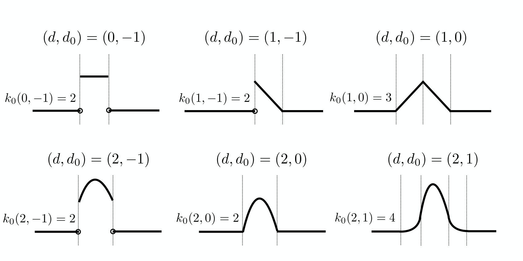
Figure 1 demonstrates the minimum number kk of pieces needed for d∈[0;2]d\in[0;2] and d0∈[−1;d−1]d_{0}\in[-1;d-1] so that a 11-sparse vector can be constructed in general position. The minimum value of kk in each scenario matches k0+1k_{0}+1 as defined in (2.2).

Refer to caption
Figure 1: Minimum number of k=k0+1k=k_{0}+1 pieces required to construct 11-sparse vectors with general position in Θ⁡(d,d0,k)\Theta(d,d_{0},k) for d∈[0;2]d\in[0;2] and d0∈[−1;d−1]d_{0}\in[-1;d-1].

3 General-order splines with shape constraint

As mentioned in (1.8) in the introduction, in contrast to the phase transition in (1.4), the faster log⁡log⁡(16​n)\log\log(16n) rate of estimation becomes universal in the class Θ∗​(0,k)\Theta^{\ast}(0,k) that contains all piecewise constant non-decreasing signals. This section derives higher-order analogues of this result. We start with the convexity constraint in the linear case in Section 3.1, and then generalize to higher-order splines in Section 3.2.

3.1 Convex piecewise linear regression

Convex regression is one of the central topics in shape constrained regression; see, e.g., [GS15, CGS15, Bel18] for global risk bounds and adaptation properties of the convex LSE.

We start by defining the function space of convex piecewise linear functions:

ℱn∗​(1,k)≡{f∈ℱn​(1,0,k):f​ has non-decreasing slopes on ​[0,1]},\displaystyle\mathcal{F}^{*}_{n}(1,k)\equiv\Big\{f\in\mathcal{F}_{n}(1,0,k):f\text{ has non-decreasing slopes on }[0,1]\Big\}, (3.1)

and the space on the sequence level:

Θn∗​(1,k)≡{θ∗∈ℝn:θi∗=f∗​(i/n)​ for some ​f∗∈ℱn∗​(1,k)},\displaystyle\Theta_{n}^{*}(1,k)\equiv\{\theta^{*}\in\mathbb{R}^{n}:\theta^{*}_{i}=f^{*}(i/n)\text{ for some }f^{*}\in\mathcal{F}^{*}_{n}(1,k)\}, (3.2)

with the subscript nn in Θn∗​(1,k)\Theta_{n}^{*}(1,k) suppressed in the sequel. The following two results show that the convexity shape constraint eliminates the phase transition in Θ⁡(1,0,k)\Theta(1,0,k).

Proposition 3.1.

Fix any θ0∈ℝn\theta_{0}\in\mathbb{R}^{n}. Let θ^∗≡θ^​(Θ∗​(1,k),Y)\widehat{\theta}^{*}\equiv\widehat{\theta}(\Theta^{*}(1,k),Y) be the LSE as defined in (1.5) under the experiment (1.1) with truth θ0\theta_{0}. Then, for any δ>0\delta>0, there exists some C=C⁡(δ)C=C(\delta) such that for any n≥n¯n\geq\underline{n} with some universal n¯\underline{n} and k≥2k\geq 2,

𝔼θ0​‖θ^∗−θ0‖2≤(1+δ)​infθ∗∈Θ∗​(1,k)‖θ∗−θ0‖2+C​σ2​k​log⁡log⁡(16​n/k).\displaystyle\mathbb{E}_{\theta_{0}}\|\widehat{\theta}^{*}-\theta_{0}\|^{2}\leq(1+\delta)\inf_{\theta^{*}\in\Theta^{*}(1,k)}\|\theta^{*}-\theta_{0}\|^{2}+C\sigma^{2}k\log\log(16n/k). (3.3)
Proposition 3.2.

Under the experiment (1.1), there exists some universal constant cc such that for all n≥n¯n\geq\underline{n} with some universal n¯\underline{n} and k≥2k\geq 2,

infθ~∗supθ∗∈Θ∗​(1,k)𝔼θ∗​‖θ~∗−θ∗‖2≥c​σ2​k​log⁡log⁡(16​n/k),\displaystyle\inf_{\widetilde{\theta}^{*}}\sup_{\theta^{*}\in\Theta^{*}(1,k)}\mathbb{E}_{\theta^{*}}\|\widetilde{\theta}^{*}-\theta^{*}\|^{2}\geq c\sigma^{2}k\log\log(16n/k),

where the infimum over θ~∗\widetilde{\theta}^{*} is taken over all measurable functions of YY.

Proposition 3.1 follows from its more general version in Theorem 3.4 ahead. The proof of Proposition 3.2 will be presented in Appedix A.2.

Remark 3.3.

The in-expectation version of Theorem 4.3 in [Bel18] proved a similar oracle inequality for the convex LSE:

𝔼θ0​‖θ^​(Θ∗,Y)−θ0‖2≤infθ∗∈Θ∗(‖θ∗−θ0‖2+C​k​(θ∗)​log⁡(e​n/k⁡(θ∗)))\displaystyle\mathbb{E}_{\theta_{0}}\|\widehat{\theta}(\Theta^{*},Y)-\theta_{0}\|^{2}\leq\inf_{\theta^{*}\in\Theta^{*}}\Big(\|\theta^{*}-\theta_{0}\|^{2}+Ck(\theta^{*})\log(en/k(\theta^{*}))\Big) (3.4)

for some universal constant C>0C>0, where Θ∗≡Θ∗​(1,n)\Theta^{*}\equiv\Theta^{*}(1,n) is the larger class of equispaced realizations of general convex functions on [0,1][0,1], and k⁡(θ∗)k(\theta^{*}) is the number of linear pieces of θ∗\theta^{*}, i.e., k⁡(θ∗)≡∑i=2n𝟏2​θi∗<θi−1∗+θi+1∗k(\theta^{*})\equiv\sum_{i=2}^{n}\bm{1}_{2\theta^{*}_{i}<\theta^{*}_{i-1}+\theta^{*}_{i+1}}. Note that Θ∗\Theta^{*}, as opposed to Θ∗​(1,k)\Theta^{*}(1,k), is a closed convex cone in ℝn\mathbb{R}^{n}. The bounds (3.3) and (3.4) are complementary in nature: the bound (3.4) exploits the convexity of Θ∗\Theta^{*} to obtain a sharp oracle inequality (in the sense of leading constant 11 before infθ∗∈Θ∗‖θ∗−θ0‖2\inf_{\theta^{*}\in\Theta^{*}}\|\theta^{*}-\theta_{0}\|^{2}), but only achieves a slower worst-case k​log⁡(e​n/k)k\log(en/k) rate over the smaller class Θ∗​(1,k)\Theta^{*}(1,k); the bound (3.3), or its adaptive version modified in a similar way as (1.6), is minimax optimal over Θ∗​(1,k)\Theta^{*}(1,k) but loses the sharp leading constant 11.

3.2 General-order spline regression with shape constraint

Following [BW07, CGS15], we consider the class of dd-monotone splines defined as follows. Let

ℱn∗​(0,k)≡{f∈ℱn​(0,−1,k):f​ is non-decreasing on ​[0,1]}\displaystyle\mathcal{F}_{n}^{*}(0,k)\equiv\Big\{f\in\mathcal{F}_{n}(0,-1,k):f\text{ is non-decreasing on }[0,1]\Big\}

be the 00-monotone class. Next, for any d∈ℤ+d\in\mathbb{Z}_{+}, define

ℱn∗(d,k)≡{\displaystyle\mathcal{F}_{n}^{*}(d,k)\equiv\Big\{ f:[0,1]→ℝ:f⁡(x)=(Ir0,…,rd−1;0d​f∘)​(x)\displaystyle f:[0,1]\to\mathbb{R}:~f(x)=(I^{d}_{r_{0},\ldots,r_{d-1};0}f_{\circ})(x)
for some f∘∈ℱn∗(0,k) and real sequence {rℓ}ℓ=0d−1}.\displaystyle\text{ for some }f_{\circ}\in\mathcal{F}_{n}^{*}(0,k)\text{ and real sequence }\{r_{\ell}\}_{\ell=0}^{d-1}\Big\}.

Define the sequence version of the above space as

Θn∗​(d,k)≡{θ∗∈ℝn:θi∗=f∗​(i/n)​ for some ​f∗∈ℱn∗​(d,k)},\displaystyle\Theta_{n}^{*}(d,k)\equiv\Big\{\theta^{*}\in\mathbb{R}^{n}:\theta^{*}_{i}=f^{*}(i/n)\text{ for some }f^{*}\in\mathcal{F}^{*}_{n}(d,k)\Big\}, (3.5)

shorthanded as Θ∗​(d,k)\Theta^{*}(d,k). One can readily check that for d=0d=0, Θ∗​(0,k)\Theta^{*}(0,k) is the class of kk-piece isotonic signals studied in [GHZ20]; for d=1d=1, Θ∗​(1,k)\Theta^{*}(1,k) coincides with the convex piecewise linear class in (3.2). Moreover, two facts follow immediately from the above definitions: (i) For any d≥1d\geq 1, f∗∈ℱn∗​(d,k)⊂Cd−1​([0,1])f^{*}\in\mathcal{F}^{*}_{n}(d,k)\subset C^{d-1}([0,1]) so that Θ∗​(d,k)⊂Θ⁡(d,d−1,k)\Theta^{*}(d,k)\subset\Theta(d,d-1,k) with the latter defined in (2.1); (ii) For any d≥1d\geq 1 and ℓ∈[1;d]\ell\in[1;d], it holds that (f∗)(ℓ)∈ℱn∗​(d−ℓ,k)(f^{*})^{(\ell)}\in\mathcal{F}^{*}_{n}(d-\ell,k).

The following result, with Proposition 3.1 as a special case, shows that dd-monotonicity eliminates the phase transition in the general spline space Θ⁡(d,d−1,k)\Theta(d,d-1,k). Its proof is given in Section 6.

Theorem 3.4.

Fix any θ0∈ℝn\theta_{0}\in\mathbb{R}^{n}. Let θ^∗≡θ^​(Θ∗​(d,k),Y)\widehat{\theta}^{*}\equiv\widehat{\theta}(\Theta^{*}(d,k),Y) be the LSE as defined in (1.5) under the experiment (1.1) with truth θ0\theta_{0}. Then, for any δ>0\delta>0, there exists some C=C⁡(d,δ)C=C(d,\delta) such that for any n≥n¯n\geq\underline{n} with some n¯=n¯​(d)\underline{n}=\underline{n}(d) and k≥2k\geq 2,

𝔼θ0​‖θ^∗−θ0‖2≤(1+δ)​infθ∗∈Θ∗​(d,k)‖θ∗−θ0‖2+C​σ2​k​log⁡log⁡(16​n/k).\displaystyle\mathbb{E}_{\theta_{0}}\|\widehat{\theta}^{*}-\theta_{0}\|^{2}\leq(1+\delta)\inf_{\theta^{*}\in\Theta^{\ast}(d,k)}\|\theta^{\ast}-\theta_{0}\|^{2}+C\sigma^{2}k\log\log(16n/k).

Moreover, there exists some c=c⁡(d)c=c(d) such that for all n≥n¯n\geq\underline{n} and k≥2k\geq 2,

infθ~∗supθ∗∈Θ∗​(d,k)𝔼θ∗​‖θ~∗−θ∗‖2≥c​σ2​log⁡log⁡(16​n),\displaystyle\inf_{\widetilde{\theta}^{*}}\sup_{\theta^{*}\in\Theta^{*}(d,k)}\mathbb{E}_{\theta^{*}}\|\widetilde{\theta}^{*}-\theta^{*}\|^{2}\geq c\sigma^{2}\log\log(16n),

where the infimum over θ~∗\widetilde{\theta}^{*} is taken over all measurable functions of YY.

Remark 3.5.

The essential technical difficulties in proving Theorem 3.4 and Proposition 3.2 over the oracle inequality version of (1.8) (cf. Theorem 2.1 of [GHZ20]) rest in the additional regularity of Θ∗​(d,k)\Theta^{*}(d,k) over Θ∗​(0,k)\Theta^{*}(0,k).

  • (i)

    For the upper bound, [GHZ20] made essential use of the fact that θ^​(Θ∗​(0,k))\widehat{\theta}(\Theta^{*}(0,k)) is the sample average given the estimated knots; cf. Lemma 5.1 therein. The analogous property is, unfortunately, not true even for θ^​(Θ∗​(1,k))\widehat{\theta}(\Theta^{*}(1,k)). Instead, we provide a completely different proof which is based on a new parametrization for general-order splines with shape constraint (cf. Lemma 6.1 ahead). We further observe that this new proof technique, when applied to the setting of [GHZ20], significantly simplifies their proof; see Section 6.3 for details.

  • (ii)

    For the lower bound in Proposition 3.2, the continuity constraint in Θ∗​(1,k)\Theta^{*}(1,k) requires a much more delicate construction of least favorable signals that achieves the k​log⁡log​(16​n/k)k\log\log(16n/k) rate, compared to Θ∗​(0,k)\Theta^{*}(0,k); see Appendix A.2 for more details. This lower bound construction can actually be extended to yield the optimal k​log⁡log​(16​n/k)k\log\log(16n/k) rate over the quadratic class Θ∗​(2,k)\Theta^{*}(2,k), but a general lower bound of the order k​log⁡log​(16​n/k)k\log\log(16n/k) is still lacking for higher-order dd-monotone splines.

4 A generalized law of iterated logarithm

In this section, we present a generalized law of iterated logarithm (LIL) in expectation that underlies the log⁡log⁡(16​n)\log\log(16n) rates derived in Sections 2 and 3. Recall that a centered random variable XX is said to be sub-Gaussian with parameter τ\tau, if there exists some K>0K>0 such that 𝔼​exp⁡(λ​X)≤K​exp⁡(λ2​τ2/2)\mathbb{E}\exp(\lambda X)\leq K\exp(\lambda^{2}\tau^{2}/2) for any λ∈ℝ\lambda\in\mathbb{R}.

Theorem 4.1.

Fix positive integers d≥1d\geq 1 and n≥2n\geq 2. Let {εi}i=1n\{\varepsilon_{i}\}_{i=1}^{n} be a sequence of independent and identically distributed centered sub-Gaussian random variables with parameter 11. Let ψ:ℝ+→ℝ+\psi:\mathbb{R}_{+}\rightarrow\mathbb{R}_{+} be a strictly increasing continuous function with inverse ψ−1\psi^{-1}. Let

Z≡max1≤n1<n2≤n⁡|∑i∈(n1;n2](i−n1)d​εi|(n2−n1)d​(n2∧(n−n1))1/2.\displaystyle Z\equiv\max_{1\leq n_{1}<n_{2}\leq n}\frac{\big|\sum_{i\in(n_{1};n_{2}]}(i-n_{1})^{d}\varepsilon_{i}\big|}{(n_{2}-n_{1})^{d}(n_{2}\wedge(n-n_{1}))^{1/2}}.

Then, provided that

∫1∞e−c0​(ψ−1​(t))2​𝑑t<∞\displaystyle\int_{1}^{\infty}e^{-c_{0}(\psi^{-1}(t))^{2}}\ \mathrm{d}t<\infty (4.1)

for some sufficiently small c0=c0​(d)c_{0}=c_{0}(d), there exist some C1=C1​(ψ,d)>0C_{1}=C_{1}(\psi,d)>0 and C2=C2​(d)>0C_{2}=C_{2}(d)>0 such that

𝔼​ψ​(Z)≤C1​[ψ⁡((C2​log⁡log⁡(16​n))1/2)∨1].\displaystyle\mathbb{E}\psi(Z)\leq C_{1}\big[\psi\big((C_{2}\log\log(16n))^{1/2}\big)\vee 1\big].

The proof of the above theorem can be found in Appendix B. Here are some choices of ψ\psi’s that will be relevant in the proofs of results in Sections 2 and 3.

Example 4.2.

Let ψ⁡(t)=tα\psi(t)=t^{\alpha} where α>0\alpha>0. Then ψ−1​(t)=t1/α\psi^{-1}(t)=t^{1/\alpha}, so clearly (4.1) holds.

Example 4.3.

Let ψ⁡(t)=ec​tα−1\psi(t)=e^{ct^{\alpha}}-1 where α,c>0\alpha,c>0. Then ψ−1​(t)=(log⁡(1+t)/c)1/α\psi^{-1}(t)=\big(\log(1+t)/c\big)^{1/\alpha}. So

∫1∞e−(c0/c2/α)​(log⁡(1+t))2/α​𝑑t\displaystyle\int_{1}^{\infty}e^{-(c_{0}/c^{2/\alpha})(\log(1+t))^{2/\alpha}}\ \mathrm{d}t {<∞,α∈(0,2],c∈(0,c0𝟏α=2+∞𝟏α∈(0,2)),=∞,otherwise.\displaystyle\begin{cases}<\infty,&\alpha\in(0,2],c\in(0,c_{0}\bm{1}_{\alpha=2}+\infty\bm{1}_{\alpha\in(0,2)}),\\ =\infty,&\textrm{otherwise}.\end{cases}

Note that a law of iterated logarithm in expectation fails in general for the choice ψ⁡(t)=ec​tα−1\psi(t)=e^{ct^{\alpha}}-1 whenever α>2\alpha>2, as α=2\alpha=2 corresponds to the maximal integrability of Gaussian random variables.

5 Proof of Theorem 2.1

Starting from this section, unless otherwise specified, we will focus on the case σ2=1\sigma^{2}=1; the extension to an arbitrary σ2>0\sigma^{2}>0 is straightforward and hence not recorded here. We will also omit the proof for the k​log⁡(e​n/k)k\log(en/k) part of Theorem 2.1 as it follows essentially from the classical arguments in [DJ94, BM01] by completely ignoring the regularity constraints. For the rest of the section, we focus on illustrating the form of k0k_{0} in (2.2) from the upper bound perspective and proving the faster log⁡log⁡(16​n)\log\log(16n) rate below the transition boundary. Section 5.1 provides a proof outline with illustrative simple cases discussed at first. Section 5.2 reduces the proof of Theorem 2.1 to the bound of complexity width in Proposition 5.2. The key ingredients to the proof of this proposition will be presented in Sections 5.3 and 5.4, followed by the main proof in Section 5.5.

5.1 Proof outline

5.1.1 Piecewise linear case

We first consider the piecewise linear case d=1,d0∈{−1,0}d=1,d_{0}\in\{-1,0\}, and assume θ0=0\theta_{0}=0 in (1.1) for simplicity of discussion. Here, the transition boundary in (2.2) is k0=2k_{0}=2 for d0=−1d_{0}=-1 and k0=3k_{0}=3 for d0=0d_{0}=0, beyond which the log⁡log⁡(16​n)\log\log(16n) rate cannot be attained. We focus on the case of k=3k=3 pieces and illustrate the difference between d0=−1d_{0}=-1 and d0=0d_{0}=0. To start, a standard reduction to complexity width in Proposition 5.1 ahead yields that for some universal constant C>0C>0,

𝔼θ0∥θ^−θ0∥2−C∥θoracle−θ0∥2≤C⋅𝔼supθ∈Θ⁡(1,d0,3):∥θ∥≤1(ε⋅θ)2≡C⋅𝔼Z2,\displaystyle\mathbb{E}_{\theta_{0}}\lVert\widehat{\theta}-\theta_{0}\rVert^{2}-C\lVert\theta_{\rm oracle}-\theta_{0}\rVert^{2}\leq C\cdot\mathbb{E}\sup_{\theta\in\Theta(1,d_{0},3):\lVert\theta\rVert\leq 1}\big(\varepsilon\cdot\theta\big)^{2}\equiv C\cdot\mathbb{E}Z^{2},

where θoracle\theta_{\rm oracle} is any oracle in Θ⁡(1,d0,3)\Theta(1,d_{0},3) such that infθ∈Θ⁡(1,d0,3)∥θ−θ0∥2\inf_{\theta\in\Theta(1,d_{0},3)}\lVert\theta-\theta_{0}\rVert^{2} is achieved, and 𝔼​Z2\mathbb{E}Z^{2} is termed the ‘complexity width’ of Θ⁡(1,d0,3)\Theta(1,d_{0},3). To bound 𝔼​Z2\mathbb{E}Z^{2}, we use the following parametrization for any given f∈ℱn​(1,d0,3)f\in\mathcal{F}_{n}(1,d_{0},3) with knots 0=n0/n≤n1/n≤n2/n≤n3/n=10=n_{0}/n\leq n_{1}/n\leq n_{2}/n\leq n_{3}/n=1: for i∈{0,1,2}i\in\{0,1,2\},

f⁡(x)=ai+bi​(x−ni/n),x∈(nin,ni+1n].\displaystyle f(x)=a_{i}+b_{i}(x-n_{i}/n),\quad x\in\bigg(\frac{n_{i}}{n},\frac{n_{i+1}}{n}\bigg]. (5.1)

Under the additional continuity constraint when d0=0d_{0}=0, one has

a1=a0+b0​(n1−n0)/n and a2=a1+b1​(n2−n1)/n.\displaystyle a_{1}=a_{0}+b_{0}(n_{1}-n_{0})/n\quad\text{ and }\quad a_{2}=a_{1}+b_{1}(n_{2}-n_{1})/n. (5.2)

Under the parametrization (5.1), the supremum within the complexity width can be bounded by

Z\displaystyle Z ≤supθ∈Θ⁡(1,d0,3):∥θ∥≤1∑i=02(|ai||∑j∈(ni;ni+1]εj|+|bin||∑j∈(ni;ni+1](j−ni)εj|).\displaystyle\leq\sup_{\theta\in\Theta(1,d_{0},3):\lVert\theta\rVert\leq 1}\sum_{i=0}^{2}\bigg(|a_{i}|\bigg\lvert\sum_{j\in(n_{i};n_{i+1}]}\varepsilon_{j}\bigg\rvert+\bigg\lvert\frac{b_{i}}{n}\bigg\rvert\bigg\lvert\sum_{j\in(n_{i};n_{i+1}]}(j-n_{i})\varepsilon_{j}\bigg\rvert\bigg).

The magnitudes of {ai}\{a_{i}\} and {bi}\{b_{i}\} can be drastically different for d0=−1d_{0}=-1 and d0=0d_{0}=0. We illustrate this on the middle piece (n1;n2](n_{1};n_{2}].

  • •

    (d0=−1d_{0}=-1). The constraint 1≥∥θ∥≥∥θ∥(n1;n2]1\geq\lVert\theta\rVert\geq\lVert\theta\rVert_{(n_{1};n_{2}]} directly yields the following estimates for a1a_{1} and b1b_{1} with some universal C>0C>0:

    |a1|≤C(n2−n1)−1/2 and |b1/n|≤C(n2−n1)−3/2.\displaystyle|a_{1}|\leq C(n_{2}-n_{1})^{-1/2}\quad\text{ and }\quad|b_{1}/n|\leq C(n_{2}-n_{1})^{-3/2}. (5.3)

    Such estimates cannot be improved for, e.g., f(x)=c(L−1/2−nL−3/2(x−1/2))𝟏(1/2,1/2+L/n](x)f(x)=c(L^{-1/2}-nL^{-3/2}(x-1/2))\bm{1}_{(1/2,1/2+L/n]}(x) for small c>0c>0 and L≥2L\geq 2.

  • •

    (d0=0d_{0}=0). With the additional continuity constraint in (5.2), refined estimates can be obtained:

    |a1|≤Cn2−1/2 and |b1/n|≤C(n2∧(n−n1))−3/2.\displaystyle|a_{1}|\leq Cn_{2}^{-1/2}\quad\text{ and }\quad|b_{1}/n|\leq C(n_{2}\wedge(n-n_{1}))^{-3/2}. (5.4)

    These estimates only hold up to k=3k=3 pieces. For k≥4k\geq 4, the best possible estimates are of type (5.3) by considering, e.g., f(x)=c(nL3/2(x−(1/2−L/n))𝟏(1/2−L/n,1/2](x)−nL3/2(x−(1/2+L/n))𝟏(1/2,L/n+1/2](x))f(x)=c\Big(nL^{3/2}\big(x-(1/2-L/n)\big)\bm{1}_{(1/2-L/n,1/2]}(x)-nL^{3/2}\big(x-(1/2+L/n)\big)\bm{1}_{(1/2,L/n+1/2]}(x)\Big) for small c>0c>0 and L≥2L\geq 2.

The crucial difference here is that estimates of type (5.4) enable a law of iterated logarithm (cf. Theorem 4.1) with 𝔼​Z2≲log⁡log⁡(16​n)\mathbb{E}Z^{2}\lesssim\log\log(16n), while those of (5.3) correspond to the maxima of O⁡(n)O(n) independent Gaussian random variables with 𝔼​Z2≲log⁡(e​n)\mathbb{E}Z^{2}\lesssim\log(en).

5.1.2 General case

Similar to the linear case discussed above, the key step is to prove

𝔼​supθ∈Θ⁡(d,d0,k0),‖θ‖≤1(ε⋅θ)2≤C​log⁡log⁡(16​n),\displaystyle\mathbb{E}\sup_{\theta\in\Theta(d,d_{0},k_{0}),\|\theta\|\leq 1}\left(\varepsilon\cdot\theta\right)^{2}\leq C\log\log(16n), (5.5)

and we need to obtain estimates of type (5.4). For simplicity, we consider the smoothest case d0=d−1d_{0}=d-1 so that k0=d+2k_{0}=d+2.

Fix a degree dd, and any f∈ℱn​(d,d−1,d+2)f\in\mathcal{F}_{n}(d,d-1,d+2) along with the corresponding θ∈Θ⁡(d,d−1,d+2)\theta\in\Theta(d,d-1,d+2) of unit norm and knots 0=n0≤n1≤…≤nd+2=n0=n_{0}\leq n_{1}\leq\ldots\leq n_{d+2}=n. We use the following parametrization of ff:

f⁡(x)=∑ℓ=1d+1aℓi​(x−nin)ℓ−1,x∈(nin,ni+1n],\displaystyle f(x)=\sum_{\ell=1}^{d+1}a^{i}_{\ell}\bigg(x-\frac{n_{i}}{n}\bigg)^{\ell-1},\quad x\in\bigg(\frac{n_{i}}{n},\frac{n_{i+1}}{n}\bigg], (5.6)

and focus on a generic piece (ni;ni+1](n_{i};n_{i+1}] at the sequence level. Here the superscript ii represents ‘the (i+1)(i+1)-th piece (ni;ni+1](n_{i};n_{i+1}]’ and the subscript ℓ\ell represents ‘the ℓ\ell-th coefficient’ in the polynomial. We aim at obtaining the following estimates:

1≥c⋅(aℓi)2​((ni+1−ni)/n)2​(ℓ−1)​(ni+1∧(n−ni)),ℓ∈[1;d+1],\displaystyle 1\geq c\cdot(a^{i}_{\ell})^{2}((n_{i+1}-n_{i})/n)^{2(\ell-1)}(n_{i+1}\wedge(n-n_{i})),\quad\ell\in[1;d+1], (5.7)

with some c=c⁡(d)c=c(d). Once these estimates are obtained, one can immediately apply Theorem 4.1 to obtain a log⁡log⁡(16​n)\log\log(16n) bound on the complexity width on (ni;ni+1](n_{i};n_{i+1}].

In (5.7), the (d−1)(d-1)-th order differentiability at each inner knot naturally divides the coefficients into two groups, the ‘shared coefficients’ {aℓi}ℓ∈[1;d]\{a_{\ell}^{i}\}_{\ell\in[1;d]} and the ‘nuisance coefficient’ ad+1ia_{d+1}^{i}. This suggests the following two-step proof strategy:

  1. (i)

    First, we show that the estimate for the second group, ad+1ia^{i}_{d+1}, follows from that of the first group; cf. Lemma 5.6 ahead.

  2. (ii)

    Second, we obtain estimates in (5.7) for ℓ∈[1;d]\ell\in[1;d] with the choice k0=d+2k_{0}=d+2; cf. Lemma 5.7 ahead.

In the proof below, we will see clearly why k0=d+2k_{0}=d+2 is the maximal number of pieces where the estimates in (5.7) are achievable. At a high level, the coefficient estimates {a⋅i}\{a_{\cdot}^{i}\} on the piece (ni;ni+1](n_{i};n_{i+1}] necessarily depend on coefficient estimates at locations to the both sides of ii. The passage of such information, for example from the rightmost knot, is precisely characterized in Lemma 5.4 ahead through a set of quadratic forms, which are obtained via ‘iterative cancellation’ to be detailed in Section 5.3. The transition boundary k0k_{0} is then determined via ‘counting of quadratic forms’ (cf. (5.15) in the main proof ahead) that mirrors the DOF calculation in (2.5), thereby unifying the heuristics in the upper and lower bounds.

5.2 Reduction to complexity width

We first introduce some notation. For any fixed θ0∈ℝn\theta_{0}\in\mathbb{R}^{n}, let θoracle≡θoracle​(θ0)∈Θ⁡(d,d0,k)\theta_{\rm oracle}\equiv\theta_{\rm oracle}(\theta_{0})\in\Theta(d,d_{0},k) be an oracle such that infθ∈Θ⁡(d,d0,k)∥θ−θ0∥\inf_{\theta\in\Theta(d,d_{0},k)}\lVert\theta-\theta_{0}\rVert is achieved, with knots 0=n0≤n1≤…≤nk=n0=n_{0}\leq n_{1}\leq\ldots\leq n_{k}=n. For each θ∈ℝn\theta\in\mathbb{R}^{n}, define θ[j]\theta_{[j]} as the sub-vector (θi)i∈(nj;nj+1](\theta_{i})_{i\in(n_{j};n_{j+1}]} and vj​(θ)≡vj​(θ,θoracle)≡(θ−θoracle)[j]/‖(θ−θoracle)[j]‖v_{j}(\theta)\equiv v_{j}(\theta;\theta_{\rm oracle})\equiv(\theta-\theta_{\rm oracle})_{[j]}/\|(\theta-\theta_{\rm oracle})_{[j]}\|.

The following result is a standard reduction principle for the LSE tailored to the class of splines. Its proof can be found in Appendix C.

Proposition 5.1.

Fix any θ0∈ℝn\theta_{0}\in\mathbb{R}^{n}. Let θ^≡θ^​(Θ⁡(d,d0,k),Y)\widehat{\theta}\equiv\widehat{\theta}(\Theta(d,d_{0},k),Y) be the LSE as defined in (1.5) under the experiment (1.1) with truth θ0\theta_{0}. Then, for any δ>0\delta>0, there exists some C=C⁡(δ)>0C=C(\delta)>0 such that

𝔼θ0∥θ^−θ0∥2≤(1+δ)∥θoracle−θ0∥2+C⋅𝔼supθ∈Θ⁡(d,d0,k)∑j=0k−1(ε[j]⋅vj(θ))2.\displaystyle\mathbb{E}_{\theta_{0}}\|\widehat{\theta}-\theta_{0}\|^{2}\leq(1+\delta)\|\theta_{\rm oracle}-\theta_{0}\|^{2}+C\cdot\mathbb{E}\sup_{\theta\in\Theta(d,d_{0},k)}\sum_{j=0}^{k-1}\big(\varepsilon_{[j]}\cdot v_{j}(\theta)\big)^{2}.

Now, note that each vj​(θ)v_{j}(\theta) is also a spline with unit norm and the same parameters (d,d0,k)(d,d_{0},k) (rigorously speaking, the two end pieces of vj​(θ)v_{j}(\theta) may have length smaller than d+1d+1, but these pieces are negligible since there are at most 2​k2k of them and each only contributes a constant (up to dd) factor to the complexity width). Therefore, in view of Proposition 5.1, the log⁡log⁡(16​n)\log\log(16n) part of Theorem 2.1 for k≤k0k\leq k_{0} is immediately implied by the following result by noticing that Θ⁡(d,d0,k)⊂Θ⁡(d,d0,k0)\Theta(d,d_{0},k)\subset\Theta(d,d_{0},k_{0}) for all k≤k0k\leq k_{0}.

Proposition 5.2.

There exists some C=C⁡(d)C=C(d) such that

𝔼​supθ∈Θ⁡(d,d0,k0),‖θ‖≤1(ε⋅θ)2≤C​log⁡log⁡(16​n).\displaystyle\mathbb{E}\sup_{\theta\in\Theta(d,d_{0},k_{0}),\|\theta\|\leq 1}\left(\varepsilon\cdot\theta\right)^{2}\leq C\log\log(16n).

The following two subsections present the main ingredients to the proof of Proposition 5.2, whose details will be presented in Section 5.5.

5.3 Groundwork

Fix any f∈ℱn​(d,d0,k0)f\in\mathcal{F}_{n}(d,d_{0},k_{0}) with knots 0=n0/n≤n1/n≤…≤nk0/n=10=n_{0}/n\leq n_{1}/n\leq\ldots\leq n_{k_{0}}/n=1 and recall the parametrization (5.6). Due to the regularity constraints, similar relations as the linear equations of the type (5.2) exist between adjacent knots. We use the notation Coef⁡[api;aqi−1]{\rm Coef}[a^{i}_{p};a^{i-1}_{q}] to denote the coefficient of aqi−1a^{i-1}_{q} in the linear equation of apia^{i}_{p}, i.e., api=∑qCoef⁡[api;aqi−1]​aqi−1a^{i}_{p}=\sum_{q}{\rm Coef}[a^{i}_{p};a^{i-1}_{q}]a^{i-1}_{q}. The following lemma makes explicit this dependence. Its proof and proofs for other lemmas in this subsection are contained in Appendix C. We write

ni;j≡(ni−nj)/n.\displaystyle n_{i;j}\equiv(n_{i}-n_{j})/n. (5.8)
Lemma 5.3.

For any i∈[1;k0−1]i\in[1;k_{0}-1], p∈[1;d0+1]p\in[1;d_{0}+1], and q∈[1;d+1]q\in[1;d+1],

Coef⁡[api;aqi−1]=(q−1p−1)​ni;i−1q−p​𝟏q≥p.\displaystyle{\rm Coef}[a^{i}_{p};a^{i-1}_{q}]={q-1\choose p-1}n_{i;i-1}^{q-p}\bm{1}_{q\geq p}.

The next Lemma 5.4 provides, as described in the proof outline in Section 5.1.2, the exact forms of the quadratic forms obtained by ‘iterative cancellation’ from right. These quadratic forms lay the foundation for coefficient estimates of type (5.7). For the rest of this section, we reserve the notation ss for the number of ‘iterative cancellation’ performed.

Before stating the general formulation in Lemma 5.4, we first present the illustrative case of cubic spline (d=3,k0=5)(d=3,k_{0}=5) in the sequence space with unit norm. We detail below the starting point (s=0)(s=0) and the first two steps of cancellation (s∈{1,2})(s\in\{1,2\}). Following the proof outline in Section 5.1.2, we separate the quadratic forms that only involve the ‘shared coefficients’ {aℓi}ℓ∈[1;3]\{a_{\ell}^{i}\}_{\ell\in[1;3]} and those that also involve the ‘nuisance coefficient’ a4ia_{4}^{i}.

  • •

    (s=0s=0). The ℓ2\ell_{2} constraint on (n4;n5](n_{4};n_{5}] for the signal (‖θ‖(n4;n5]≤‖θ‖=1\|\theta\|_{(n_{4};n_{5}]}\leq\|\theta\|=1) provides control on the following 44 quadratic forms of length 11:

    1≥c⋅[{(n−n4)​(a14)2+(n−n4)3n2​(a24)2+(n−n4)5n4​(a34)2}+(n−n4)7n6​(a44)2].\displaystyle 1\geq c\cdot\bigg[\Big\{(n-n_{4})(a^{4}_{1})^{2}+\frac{(n-n_{4})^{3}}{n^{2}}(a^{4}_{2})^{2}+\frac{(n-n_{4})^{5}}{n^{4}}(a^{4}_{3})^{2}\Big\}+\frac{(n-n_{4})^{7}}{n^{6}}(a^{4}_{4})^{2}\bigg].
  • •

    (s=1s=1). For the first cancellation, we have, by Lemma 5.3,

    (a14a24a34)=(1n4;3n4;32n4;33012​n4;33​n4;320013​n4;3)​(a13a23a33a43).\displaystyle\begin{pmatrix}a_{1}^{4}\\ a_{2}^{4}\\ a_{3}^{4}\end{pmatrix}=\begin{pmatrix}1&n_{4;3}&n_{4;3}^{2}&n_{4;3}^{3}\\ 0&1&2n_{4;3}&3n_{4;3}^{2}\\ 0&0&1&3n_{4;3}\end{pmatrix}\begin{pmatrix}a_{1}^{3}\\ a_{2}^{3}\\ a_{3}^{3}\\ a_{4}^{3}\end{pmatrix}. (5.9)

    The identity (5.9) enables us to first find a linear combination of (a24,a34)(a^{4}_{2},a^{4}_{3}) to cancel a43a^{3}_{4}, and then to find another linear combination of (a14,a24,a34)(a^{4}_{1},a^{4}_{2},a^{4}_{3}) to cancel both a33a^{3}_{3} and a43a^{3}_{4}. These, along with direct expansion of the term (a34)2​(n−n4)5/n4(a^{4}_{3})^{2}(n-n_{4})^{5}/n^{4} using (5.9), leave us with 33 quadratic forms of length 22:

    1≥c⋅[{(n−n4)​(3​a13+n4;3​a23)2+(n−n4)3n2​(a23+n4;3​a33)2}+(n−n4)5n4​(a33+3​n4;3​a43)2].\displaystyle 1\geq c\cdot\bigg[\Big\{(n-n_{4})\big(3a^{3}_{1}+n_{4;3}a^{3}_{2}\big)^{2}+\frac{(n-n_{4})^{3}}{n^{2}}\big(a^{3}_{2}+n_{4;3}a^{3}_{3}\big)^{2}\Big\}+\frac{(n-n_{4})^{5}}{n^{4}}\big(a^{3}_{3}+3n_{4;3}a^{3}_{4}\big)^{2}\bigg].
  • •

    (s=2s=2). For the second cancellation, we have, by Lemma 5.3 again,

    (a13a23a33)=(1n3;2n3;22n3;23012​n3;23​n3;220013​n3;2)​(a12a22a32a42).\displaystyle\begin{pmatrix}a_{1}^{3}\\ a_{2}^{3}\\ a_{3}^{3}\end{pmatrix}=\begin{pmatrix}1&n_{3;2}&n_{3;2}^{2}&n_{3;2}^{3}\\ 0&1&2n_{3;2}&3n_{3;2}^{2}\\ 0&0&1&3n_{3;2}\end{pmatrix}\begin{pmatrix}a_{1}^{2}\\ a_{2}^{2}\\ a_{3}^{2}\\ a_{4}^{2}\end{pmatrix}.

    Then, finding a linear combination of (a13,a23,a33)(a^{3}_{1},a^{3}_{2},a^{3}_{3}) to cancel a42a^{2}_{4} and directly expanding (a23+n4;3​a33)2​(n−n4)3/n2\big(a^{3}_{2}+n_{4;3}a^{3}_{3}\big)^{2}(n-n_{4})^{3}/n^{2}, we obtain 22 quadratic forms of length 33:

    1≥c⋅\displaystyle 1\geq c\cdot [(n−n4)(3a21+(2n3;2+n4;3)a22+(n3;22+n3;2n4;3)a23)2\displaystyle\bigg[(n-n_{4})\bigg(3a^{2}_{1}+(2n_{3;2}+n_{4;3})a^{2}_{2}+(n_{3;2}^{2}+n_{3;2}n_{4;3})a^{2}_{3}\bigg)^{2}
    +(n−n4)3n2(a22+(2n3;2+n4;3)a23+(3n3;22+3n3;2n4;3)a24)2].\displaystyle+\frac{(n-n_{4})^{3}}{n^{2}}\bigg(a^{2}_{2}+(2n_{3;2}+n_{4;3})a^{2}_{3}+(3n_{3;2}^{2}+3n_{3;2}n_{4;3})a^{2}_{4}\bigg)^{2}\bigg].

To state the above cancellation scheme for general dd and d0d_{0}, some further notation is introduced. Fix d,d0d,d_{0}, and the resulting k0k_{0} as defined in (2.2). Define the sequence {β¯js}\{\overline{\beta}^{s}_{j}\}, s∈[0;⌊(d0+1)/(d−d0)⌋]s\in[0;\left\lfloor(d_{0}+1)/(d-d_{0})\right\rfloor] recursively as follows. Let β¯0s≡1\overline{\beta}^{s}_{0}\equiv 1,

β¯js\displaystyle\overline{\beta}^{s}_{j} ≡∑ℓ=0j(s⁡(d−d0)−ℓj−ℓ)​nk0−s;k0−1−sj−ℓ​β¯ℓs−1\displaystyle\equiv\sum_{\ell=0}^{j}\binom{s(d-d_{0})-\ell}{j-\ell}n_{k_{0}-s;k_{0}-1-s}^{j-\ell}\overline{\beta}_{\ell}^{s-1} (5.10)

for j∈[1;s⁡(d−d0)]j\in[1;s(d-d_{0})], and β¯js≡0\overline{\beta}^{s}_{j}\equiv 0 for j>s⁡(d−d0)j>s(d-d_{0}). Further define, for every i∈[1;(s+1)​d0−s​d+1]i\in[1;(s+1)d_{0}-sd+1] and j∈[0;s⁡(d−d0)]j\in[0;s(d-d_{0})],

D⁡(i,0)≡1,D⁡(i,j)≡⊙¯​(i,j)⊙¯​(d+1−i,j) for ​j≥1.D(i,0)\equiv 1,\quad D(i,j)\equiv\frac{\overline{\odot}(i;j)}{\underline{\odot}(d+1-i;j)}\quad\text{ for }j\geq 1.

Lastly, let β¯i,js≡D⁡(i,j)​β¯js\overline{\beta}^{s}_{i,j}\equiv D(i,j)\overline{\beta}^{s}_{j}.

We work under the extra condition that

n1;0∧nk0;k0−1≥max⁡{n2;1,…,nk0−1;k0−2}.\displaystyle n_{1;0}\wedge n_{k_{0};k_{0}-1}\geq\max\{n_{2;1},\ldots,n_{k_{0}-1;k_{0}-2}\}. (5.11)

We remark that condition (5.11) is made merely for presentational simplicity; see the comments after Lemma 5.7 ahead for detailed discussion of this condition.

Lemma 5.4.

Suppose (5.11) holds. Fix dd, d0d_{0}, and k0k_{0} as defined in (2.2), and any θ∈Θ⁡(d,d0,k0)\theta\in\Theta(d,d_{0},k_{0}) such that ‖θ‖≤1\|\theta\|\leq 1. Then, there exists some c=c⁡(d)c=c(d) such that, for any s∈[0;⌊(d0+1)/(d−d0)⌋]s\in[0;\left\lfloor(d_{0}+1)/(d-d_{0})\right\rfloor],

1\displaystyle 1 ≥c{∑i=1(s+1)​d0−s​d+1+∑i=(s+1)​d0−s​d+2s​d0−(s−1)​d+1}(n−nk0−1)2​i−1n2​(i−1)(∑j=0s⁡(d−d0)β¯i,jsai+jk0−1−s)2.\displaystyle\geq c\bigg\{\sum_{i=1}^{(s+1)d_{0}-sd+1}+\sum_{i=(s+1)d_{0}-sd+2}^{sd_{0}-(s-1)d+1}\bigg\}\frac{(n-n_{k_{0}-1})^{2i-1}}{n^{2(i-1)}}\bigg(\sum_{j=0}^{s(d-d_{0})}\overline{\beta}_{i,j}^{s}a_{i+j}^{k_{0}-1-s}\bigg)^{2}. (5.12)
Remark 5.5.

Several remarks for the quadratic forms above are in order.

  • (i)

    The quadratic forms in (5.12) are obtained via iterative cancellation from knot nk0−1n_{k_{0}-1}.

  • (ii)

    In a generic β¯i,js\overline{\beta}^{s}_{i,j}, the superscript ss marks the counts of cancellations already performed, ii indicates the ii-th quadratic form, and jj indicates the coefficient for the jj-th component in this quadratic form.

  • (iii)

    In (5.12), we intentionally separate the indices i∈[1;(s+1)​d0−s​d+1]i\in[1;(s+1)d_{0}-sd+1] and i∈[(s+1)​d0−s​d+2;s​d0−(s−1)​d+1]i\in[(s+1)d_{0}-sd+2;sd_{0}-(s-1)d+1] since the first set of quadratic forms only involves the ‘shared coefficients’ aj⋅a^{\cdot}_{j} with j∈[1;d0+1]j\in[1;d_{0}+1].

  • (iv)

    Every time ss grows by 11, the first summand of (5.12) has (d−d0)(d-d_{0}) fewer quadratic forms with each one comprising of (d−d0)(d-d_{0}) more components.

5.4 Key estimates

Recall the coefficient sequence {aℓi}i∈[0;k0−1],ℓ∈[1;d+1]\{a^{i}_{\ell}\}_{i\in[0;k_{0}-1],\ell\in[1;d+1]} defined in (5.6). As described in Section 5.1, we aim to obtain sharp estimates of type (5.7). For any a,b∈[1;n]a,b\in[1;n], define

M⁡(a,b)≡(a∧(n−b))1/2.\displaystyle M(a,b)\equiv(a\wedge(n-b))^{1/2}.

The first result below reduces the task of obtaining (5.7) for all the coefficients down to estimating only the ‘shared coefficients’ {aℓ⋅}ℓ∈[1;d0+1]\{a^{\cdot}_{\ell}\}_{\ell\in[1;d_{0}+1]}, from which the estimates for ‘nuisance coefficients’ {aℓ⋅}ℓ∈[d0+2;d+1]\{a^{\cdot}_{\ell}\}_{\ell\in[d_{0}+2;d+1]} can be derived. Its proof can be found in Appendix C.

Lemma 5.6.

Fix any i∈[1;k0−2]i\in[1;k_{0}-2]. Suppose there exists some c=c⁡(d)c=c(d) such that for every ℓ∈[1;d0+1]\ell\in[1;d_{0}+1], it holds that 1≥c​(aℓi)2​ni+1,i2​(ℓ−1)​M2​(ni+1,ni)1\geq c(a^{i}_{\ell})^{2}n_{i+1,i}^{2(\ell-1)}M^{2}(n_{i+1},n_{i}). Then, there exists some c′=c′​(d)c^{\prime}=c^{\prime}(d) such that

1≥c′​(aℓi)2​ni+1,i2​(ℓ−1)​M2​(ni+1,ni)\displaystyle 1\geq c^{\prime}(a^{i}_{\ell})^{2}n_{i+1,i}^{2(\ell-1)}M^{2}(n_{i+1},n_{i})

for every ℓ∈[d0+2;d+1]\ell\in[d_{0}+2;d+1].

Following the preceding lemma, the next result, which builds on the groundwork derived in Lemma 5.4, makes use of an inductive argument to derive sharp estimates of the type (5.7) for {aℓi+1}ℓ∈[1;d0+1]\{a^{i+1}_{\ell}\}_{\ell\in[1;d_{0}+1]} on a fixed target piece (ni+1;ni+2](n_{i+1};n_{i+2}]. To make the notation more accessible, we present here the special case d0=d−1d_{0}=d-1 (so that k0=d+2k_{0}=d+2) and defer the case of general d0d_{0} to Appendix C.5.

Lemma 5.7.

Suppose d0=d−1d_{0}=d-1 and (5.11) holds. Fix i∈[0;d−1]i\in[0;d-1]. For some c=c⁡(d)c=c(d), the following estimates hold for all locations 1≤j≤i+11\leq j\leq i+1:

1\displaystyle 1 ≥c​max1≤ℓ≤d​{(aℓj)2⋅ni+2;j2​{(d−i)∧(ℓ−1)}⋅(∏k=d−i+2(d−j+2)∧ℓnd+3−k;j2)⋅nj+1;j2​(ℓ−(d−j+2))+⋅M2​(nj+1,nj)}.\displaystyle\geq c\max_{1\leq\ell\leq d}\bigg\{(a^{j}_{\ell})^{2}\cdot n_{i+2;j}^{2\{(d-i)\wedge(\ell-1)\}}\cdot\bigg(\prod_{k=d-i+2}^{(d-j+2)\wedge\ell}n^{2}_{d+3-k;j}\bigg)\cdot n_{j+1;j}^{2(\ell-(d-j+2))_{+}}\cdot M^{2}(n_{j+1},n_{j})\bigg\}.

Here ∏k=k1k2≡1\prod_{k=k_{1}}^{k_{2}}\equiv 1 for k2<k1k_{2}<k_{1}. In particular, for j=i+1j=i+1:

1\displaystyle 1 ≥c​max1≤ℓ≤d​{(aℓi+1)2⋅ni+2;i+12​(ℓ−1)⋅M2​(ni+2,ni+1)}.\displaystyle\geq c\max_{1\leq\ell\leq d}\bigg\{(a^{i+1}_{\ell})^{2}\cdot n_{i+2;i+1}^{2(\ell-1)}\cdot M^{2}(n_{i+2},n_{i+1})\bigg\}. (5.13)

The proof of the above lemma is presented in the next subsection. We emphasize that the condition (5.11) is made only for presentational simplicity, as we explain below. If it does not hold, we can adopt the following partition of the pieces {(n0;n1],…,(nd+1;nd+2]}\{(n_{0};n_{1}],\ldots,(n_{d+1};n_{d+2}]\} via general length constraints. Fix a target piece (ni+1;ni+2](n_{i+1};n_{i+2}] with i∈[0;d−1]i\in[0;d-1].

  • S1.

    First locate among all pieces the longest one denoted as (ni1∗;ni1∗+1](n_{i^{*}_{1}};n_{i^{*}_{1}+1}] with i1∗∈[0;d+1]i_{1}^{*}\in[0;d+1]. If this is the target piece, then we can directly apply Lemma E.1 in Appendix E to this piece to obtain the desired estimates in (5.13).

  • S2.

    If not, assume without loss of generality that the target piece is to the left of this longest piece, i.e., i+1<i1∗i+1<i^{*}_{1}. Then, we can locate the longest piece among {(n0;n1],…,(ni1∗−1;ni1∗]}\{(n_{0};n_{1}],\ldots,(n_{i_{1}^{*}-1};n_{i_{1}^{*}}]\}, which we denote as (ni2∗;ni2∗+1](n_{i_{2}^{*}};n_{i_{2}^{*}+1}] with i2∗∈[0;i1∗−1]i_{2}^{*}\in[0;i_{1}^{*}-1]. If the target piece is among {(ni2∗;ni2∗+1],…,(ni1∗−1;ni1∗]}\{(n_{i_{2}^{*}};n_{i_{2}^{*}+1}],\ldots,(n_{i_{1}^{*}-1};n_{i_{1}^{*}}]\}, we can then make the following two modifications of Lemmas 5.4 and 5.7: (i) choose location ni1∗n_{i^{*}_{1}} (instead of the current nd+1n_{d+1}) as the starting point for the cancellation of the quadratic forms; (ii) choose location i2∗+1i_{2}^{*}+1 (instead of the current location 11) as the starting point for the induction in Lemma 5.7. These two modifications will yield the desired estimates for {aℓi+1}\{a^{i+1}_{\ell}\} in (5.13).

  • S3.

    If this is not the case, i.e., (ni+1;ni+2]∈{(n1;n2],…,(ni2∗−1;ni2∗]}(n_{i+1};n_{i+2}]\in\{(n_{1};n_{2}],\ldots,(n_{i_{2}^{*}-1};n_{i_{2}^{*}}]\}, we can then iterate S2 with i2∗i_{2}^{*} in place of i1∗i_{1}^{*}. This partitioning will terminate in a finite number of steps.

Condition (5.11) (with n1;0≤nd+2;d+1n_{1;0}\leq n_{d+2;d+1}), along with the current versions of Lemmas 5.4 and 5.7, correspond to the above partitioning scheme with an early stop at S2 with i1∗=d+1i_{1}^{*}=d+1 and i2∗=0i_{2}^{*}=0. On the other hand, condition (5.11) represents the most difficult case in the sense that the maximal gap i1∗−i2∗=d+1i_{1}^{*}-i_{2}^{*}=d+1 activates the condition k≤k0=d+2k\leq k_{0}=d+2 as seen in (5.15) in the proof ahead.

5.5 Main proof

The main step in the proof of Proposition 5.2 is the set of coefficient estimates in Lemma 5.7, with its more general version stated in Appendix C.5. We present the proof of this lemma in the special case d0=d−1d_{0}=d-1; the proof for the general case is completely analogous.

Proof of Lemma 5.7.

Let

Qj2​(ℓ)=ni+2;j2​{(d−i)∧(ℓ−1)}⋅(∏k=d−i+2(d−j+2)∧ℓnd+3−k;j2)⋅nj+1;j2​(ℓ−(d−j+2))+.\displaystyle Q_{j}^{2}(\ell)=n_{i+2;j}^{2\{(d-i)\wedge(\ell-1)\}}\cdot\bigg(\prod_{k=d-i+2}^{(d-j+2)\wedge\ell}n^{2}_{d+3-k;j}\bigg)\cdot n_{j+1;j}^{2(\ell-(d-j+2))_{+}}.

For the rest of the proof, empty ∏\prod is to be understood as 11 and empty ⋁\bigvee is to be understood as 00. We will prove (a slightly stronger version with M⁡(n1,n0)M(n_{1},n_{0}) instead of M⁡(nj+1,nj)M(n_{j+1},n_{j}))

1\displaystyle 1 ≳max1≤ℓ≤d⁡{(aℓj)2​Qj2​(ℓ)}⋅M2​(n1,n0)\displaystyle\gtrsim\max_{1\leq\ell\leq d}\big\{(a_{\ell}^{j})^{2}Q_{j}^{2}(\ell)\big\}\cdot M^{2}(n_{1},n_{0}) (5.14)

by induction on j∈[1;i+1]j\in[1;i+1]. The baseline case j=1j=1 clearly holds by the condition (5.11) and application of Lemma E.1 to the piece (n0;n1](n_{0};n_{1}]. Now, suppose the induction holds up to some location j∈[1;i]j\in[1;i], and we will prove the iteration at location j+1j+1.

(Part I). We deal with {aℓj+1}ℓ=1d−j+1\{a^{j+1}_{\ell}\}_{\ell=1}^{d-j+1} in this part. For this, we first obtain estimates for ad+1ja^{j}_{d+1} and then use triangle inequality. Applying Lemma 5.4 with d0=d−1d_{0}=d-1 and s=d−js=d-j, the jj-th term in the first summand therein yields that

1≳\displaystyle 1\gtrsim (n−nd+1)2​j−1n2​(j−1)​(∑ℓ=0d−jβ¯j,ℓd−j​aj+ℓj+1)2\displaystyle\frac{(n-n_{d+1})^{2j-1}}{n^{2(j-1)}}\bigg(\sum_{\ell=0}^{d-j}\overline{\beta}_{j,\ell}^{d-j}a_{j+\ell}^{j+1}\bigg)^{2}
=(n−nd+1)2​j−1n2​(j−1)​(∑ℓ=0d−jβ¯j,ℓd−j​∑k=ℓd−j+1(k+j−1ℓ+j−1)​nj+1;jk−ℓ​ak+jj)2\displaystyle=\frac{(n-n_{d+1})^{2j-1}}{n^{2(j-1)}}\bigg(\sum_{\ell=0}^{d-j}\overline{\beta}_{j,\ell}^{d-j}\sum_{k=\ell}^{d-j+1}\binom{k+j-1}{\ell+j-1}n_{j+1;j}^{k-\ell}a_{k+j}^{j}\bigg)^{2}
≡(n−nd+1)2​j−1n2​(j−1)​(∑k=0d−j+1γ¯j,kd−j+1​ak+jj)2,\displaystyle\equiv\frac{(n-n_{d+1})^{2j-1}}{n^{2(j-1)}}\bigg(\sum_{k=0}^{d-j+1}\bar{\gamma}_{j,k}^{d-j+1}a_{k+j}^{j}\bigg)^{2},

where we used Lemma 5.3 and γ¯j,kd−j+1≡∑q=0(d−j)∧kβ¯j,qd−j​(k+j−1q+j−1)​nj+1;jk−q\bar{\gamma}_{j,k}^{d-j+1}\equiv\sum_{q=0}^{(d-j)\wedge k}\overline{\beta}_{j,q}^{d-j}\binom{k+j-1}{q+j-1}n_{j+1;j}^{k-q}. Note that for a generic number of kk pieces, when j=1j=1, we need to take d0=d−1d_{0}=d-1 and s=(k−1)−(j+1)=k−3s=(k-1)-(j+1)=k-3 in Lemma 5.4, in which case the first summand is non-void if and only if

d−s=d−k+3≥1⇔k≤d+2.\displaystyle d-s=d-k+3\geq 1\iff k\leq d+2. (5.15)

This explains the transition boundary k0=d+2k_{0}=d+2 as in (2.2).

Combining the above estimate with the estimates for {akj}k=jd\{a^{j}_{k}\}_{k=j}^{d} from the induction assumption, and using Lemma E.2 to cancel everything but ad+1ja_{d+1}^{j}, we have

1\displaystyle 1 ≳(n−nd+1)2​j−1n2​(j−1)​(∑k=0d−j+1γ¯j,kd−j+1​ak+jj)2+∑k=jd[(akj)2⋅Qj2​(k)⋅M2​(n1,n0)]\displaystyle\gtrsim\frac{(n-n_{d+1})^{2j-1}}{n^{2(j-1)}}\bigg(\sum_{k=0}^{d-j+1}\bar{\gamma}_{j,k}^{d-j+1}a_{k+j}^{j}\bigg)^{2}+\sum_{k=j}^{d}\bigg[(a^{j}_{k})^{2}\cdot Q_{j}^{2}(k)\cdot M^{2}(n_{1},n_{0})\bigg]
≳(ad+1j)2​{(n−nd+1)2​j−1​(γ¯j,d−j+1d−j+1)2n2​(j−1)∧⋀k=jd[Qj2​(k)​M2​(n1,n0)​(γ¯j,d−j+1d−j+1)2(γ¯j,k−jd−j+1)2]}\displaystyle\gtrsim\big(a_{d+1}^{j}\big)^{2}\bigg\{\frac{(n-n_{d+1})^{2j-1}(\bar{\gamma}_{j,d-j+1}^{d-j+1})^{2}}{n^{2(j-1)}}\wedge\bigwedge_{k=j}^{d}\bigg[Q_{j}^{2}(k)M^{2}(n_{1},n_{0})\frac{(\bar{\gamma}_{j,d-j+1}^{d-j+1})^{2}}{(\bar{\gamma}_{j,k-j}^{d-j+1})^{2}}\bigg]\bigg\}
≡(ad+1j)2​{Aj∧⋀k=jdBj,k}.\displaystyle\equiv\big(a_{d+1}^{j}\big)^{2}\bigg\{A_{j}\wedge\bigwedge_{k=j}^{d}B_{j,k}\bigg\}.

As Aj/(γ¯j,d−j+1d−j+1)2=nd+2;d+12​(j−1)​(n−nd+1)≳Bj,j/(γ¯j,d−j+1d−j+1)2A_{j}/(\bar{\gamma}_{j,d-j+1}^{d-j+1})^{2}=n_{d+2;d+1}^{2(j-1)}(n-n_{d+1})\gtrsim B_{j,j}/(\bar{\gamma}_{j,d-j+1}^{d-j+1})^{2} by the assumption that the two end pieces are longer than any middle pieces, we only need to bound from below ∧k=jdBj,k\wedge_{k=j}^{d}B_{j,k}. By definition of γ¯⋅,⋅⋅\bar{\gamma}_{\cdot,\cdot}^{\cdot} and non-negativity of β¯⋅,⋅⋅\overline{\beta}^{\cdot}_{\cdot,\cdot}, for any j≤k≤dj\leq k\leq d,

(γ¯j,d−j+1d−j+1)2(γ¯j,k−jd−j+1)2\displaystyle\frac{(\bar{\gamma}_{j,d-j+1}^{d-j+1})^{2}}{(\bar{\gamma}_{j,k-j}^{d-j+1})^{2}} ≍(∑q=0d−jβ¯j,qd−j​nj+1;j(d−j+1)−q)2(∑q=0k−jβ¯j,qd−j​nj+1;jk−j−q)2(by definition)\displaystyle\asymp\frac{\big(\sum_{q=0}^{d-j}\overline{\beta}_{j,q}^{d-j}n_{j+1;j}^{(d-j+1)-q}\big)^{2}}{\big(\sum_{q=0}^{k-j}\overline{\beta}_{j,q}^{d-j}n_{j+1;j}^{k-j-q}\big)^{2}}\quad(\textrm{by definition})
≍⋁p=0d−k⋁q=0k−j(β¯j,p+qd−j)2​nj+1;j2​{(d−j+1)−(p+q)}⋁q=0k−j(β¯j,qd−j)2​nj+1;j2​(k−j−q)(by rearranging the numerator)\displaystyle\asymp\bigvee_{p=0}^{d-k}\frac{\bigvee_{q=0}^{k-j}(\overline{\beta}_{j,p+q}^{d-j})^{2}n_{j+1;j}^{2\{(d-j+1)-(p+q)\}}}{\bigvee_{q=0}^{k-j}(\overline{\beta}_{j,q}^{d-j})^{2}n_{j+1;j}^{2(k-j-q)}}\quad(\textrm{by rearranging the numerator})
≥⋁p=0d−k{nj+1;j2​(d−k+1−p)⋀q=0k−j(β¯j,p+qd−jβ¯j,qd−j)2}(by Lemma E.2)\displaystyle\geq\bigvee_{p=0}^{d-k}\bigg\{n_{j+1;j}^{2(d-k+1-p)}\bigwedge_{q=0}^{k-j}\bigg(\frac{\overline{\beta}_{j,p+q}^{d-j}}{\overline{\beta}_{j,q}^{d-j}}\bigg)^{2}\bigg\}\quad(\textrm{by Lemma \ref{lemma:wedge}})
≳⋁p=0d−k{nj+1;j2​(d−k+1−p)⋀q=0k−j∏r=1+qp+qnd+2−r;j+12}(by Lemma E.7)\displaystyle\gtrsim\bigvee_{p=0}^{d-k}\bigg\{n_{j+1;j}^{2(d-k+1-p)}\bigwedge_{q=0}^{k-j}\prod_{r=1+q}^{p+q}n_{d+2-r;j+1}^{2}\bigg\}\quad(\textrm{by Lemma \ref{lemma:property_beta}})
=⋁p=0d−k{nj+1;j2​(d−k+1−p)∏r=1+k−jp+k−jnd+2−r;j+12}(minimum at q=k−j).\displaystyle=\bigvee_{p=0}^{d-k}\bigg\{n_{j+1;j}^{2(d-k+1-p)}\prod_{r=1+k-j}^{p+k-j}n_{d+2-r;j+1}^{2}\bigg\}\quad(\textrm{minimum at }q=k-j).

Hence

1≳(ad+1j)2​[⋀k=jdQj2​(k)​⋁p=0d−k{nj+1;j2​(d−k+1−p)​∏r=1+k−jp+k−jnd+2−r;j+12}]​M2​(n1,n0).\displaystyle 1\gtrsim(a_{d+1}^{j})^{2}\bigg[\bigwedge_{k=j}^{d}Q_{j}^{2}(k)\bigvee_{p=0}^{d-k}\bigg\{n_{j+1;j}^{2(d-k+1-p)}\prod_{r=1+k-j}^{p+k-j}n_{d+2-r;j+1}^{2}\bigg\}\bigg]M^{2}(n_{1},n_{0}).

This implies that for 1≤ℓ≤d1\leq\ell\leq d, by taking p=(ℓ−k)+p=(\ell-k)_{+} above and Lemma 5.3,

M⁡(n1,n0)|aℓj+1|≲M⁡(n1,n0)​[∑k=ℓdnj+1;jk−ℓ​|akj|+nj+1;jd+1−ℓ​|ad+1j|]\displaystyle M(n_{1},n_{0})|a^{j+1}_{\ell}|\lesssim M(n_{1},n_{0})\bigg[\sum_{k=\ell}^{d}n_{j+1;j}^{k-\ell}|a^{j}_{k}|+n_{j+1;j}^{d+1-\ell}|a^{j}_{d+1}|\bigg]
≲∑k=ℓdnj+1;jk−ℓ​Qj−1​(k)+⋁k=jd{Qj−1​(k)​nj+1;jk−ℓ+(ℓ−k)+​∏r=1(ℓ−k)+nd+2+j−k−r;j+1−1}\displaystyle\lesssim\sum_{k=\ell}^{d}n_{j+1;j}^{k-\ell}Q_{j}^{-1}(k)+\bigvee_{k=j}^{d}\bigg\{Q_{j}^{-1}(k)n_{j+1;j}^{k-\ell+(\ell-k)_{+}}\prod_{r=1}^{(\ell-k)_{+}}n_{d+2+j-k-r;j+1}^{-1}\bigg\}
=∑k=ℓdnj+1;jk−ℓ​Qj−1​(k)+⋁j≤k<ℓ∨j{Qj−1​(k)​∏r=1ℓ∨j−knd+2+j−k−r;j+1−1}+⋁ℓ∨j≤k≤d{Qj−1​(k)​nj+1;jk−ℓ}.\displaystyle=\sum_{k=\ell}^{d}n_{j+1;j}^{k-\ell}Q_{j}^{-1}(k)+\bigvee_{j\leq k<\ell\vee j}\bigg\{Q_{j}^{-1}(k)\prod_{r=1}^{\ell\vee j-k}n_{d+2+j-k-r;j+1}^{-1}\bigg\}+\bigvee_{\ell\vee j\leq k\leq d}\bigg\{Q_{j}^{-1}(k)n^{k-\ell}_{j+1;j}\bigg\}.

Using that k↦nj+1;jk−ℓ​Qj−1​(k)k\mapsto n_{j+1;j}^{k-\ell}Q_{j}^{-1}(k) is non-increasing, the first and third terms in the above display are on the same order as Qj−1​(ℓ)+Qj−1​(ℓ∨j)​nj+1;jℓ∨j−ℓ≍Qj−1​(ℓ)Q_{j}^{-1}(\ell)+Q_{j}^{-1}(\ell\vee j)n_{j+1;j}^{\ell\vee j-\ell}\asymp Q_{j}^{-1}(\ell). Hence we only need to verify for all 1≤ℓ≤d−j+11\leq\ell\leq d-j+1, 1≤j≤i1\leq j\leq i,

𝔔j,1​(ℓ)+𝔔j,2​(ℓ)≡Qj−1​(ℓ)+⋁j≤k<ℓ∨j{Qj−1​(k)​∏r=1ℓ∨j−knd+2+j−k−r;j+1−1}≲Qj+1−1​(ℓ).\displaystyle\mathfrak{Q}_{j,1}(\ell)+\mathfrak{Q}_{j,2}(\ell)\equiv Q_{j}^{-1}(\ell)+\bigvee_{j\leq k<\ell\vee j}\bigg\{Q_{j}^{-1}(k)\prod_{r=1}^{\ell\vee j-k}n_{d+2+j-k-r;j+1}^{-1}\bigg\}\lesssim Q_{j+1}^{-1}(\ell). (5.16)

(Case 1). If 1≤ℓ≤d−i+11\leq\ell\leq d-i+1, Qj−1​(ℓ)=ni+2;j−(ℓ−1)Q_{j}^{-1}(\ell)=n_{i+2;j}^{-(\ell-1)} and Qj−1​(ℓ)=ni+2;j+1−(ℓ−1)Q_{j}^{-1}(\ell)=n_{i+2;j+1}^{-(\ell-1)}, so:

  • •

    (first term) 𝔔j,1​(ℓ)=ni+2;j−(ℓ−1)≤ni+2;j+1−(ℓ−1)=Qj+1−1​(ℓ)\mathfrak{Q}_{j,1}(\ell)=n_{i+2;j}^{-(\ell-1)}\leq n_{i+2;j+1}^{-(\ell-1)}=Q_{j+1}^{-1}(\ell).

  • •

    (second term) without loss of generality we assume ℓ>j\ell>j (otherwise this term does not exist):

    𝔔j,2​(ℓ)\displaystyle\mathfrak{Q}_{j,2}(\ell) =⋁j≤k<ℓ{ni+2;j−(k−1)​∏r=1ℓ−knd+2+j−k−r;j+1−1}\displaystyle=\bigvee_{j\leq k<\ell}\bigg\{n_{i+2;j}^{-(k-1)}\prod_{r=1}^{\ell-k}n_{d+2+j-k-r;j+1}^{-1}\bigg\}
    ≤⋁j≤k<ℓ{ni+2;j−(k−1)​nd+2+j−ℓ;j+1−(ℓ−k)}\displaystyle\leq\bigvee_{j\leq k<\ell}\bigg\{n_{i+2;j}^{-(k-1)}n_{d+2+j-\ell;j+1}^{-(\ell-k)}\bigg\}
    ≤⋁j≤k<ℓ{ni+2;j+1−(k−1)​ni+2;j+1−(ℓ−k)}=ni+2;j+1−(ℓ−1)=Qj+1−1​(ℓ),\displaystyle\leq\bigvee_{j\leq k<\ell}\bigg\{n_{i+2;j+1}^{-(k-1)}n_{i+2;j+1}^{-(\ell-k)}\bigg\}=n_{i+2;j+1}^{-(\ell-1)}=Q_{j+1}^{-1}(\ell),

    where the first equality follows since k<ℓ≤d−i+1k<\ell\leq d-i+1 so that Qj−1​(k)=ni+2;j−(k−1)Q^{-1}_{j}(k)=n_{i+2;j}^{-(k-1)}, and the second inequality follows by noting that ℓ≤d−i+1\ell\leq d-i+1 implies d+2+j−ℓ≥i+2d+2+j-\ell\geq i+2.

(Case 2). If d−i+2≤ℓ≤d−j+1d-i+2\leq\ell\leq d-j+1, Qj−1​(ℓ)=ni+2;j−(d−i)​∏s=d−i+2ℓnd+3−s;j−1Q_{j}^{-1}(\ell)=n_{i+2;j}^{-(d-i)}\prod_{s=d-i+2}^{\ell}n_{d+3-s;j}^{-1} and Qj+1−1​(ℓ)=ni+2;j+1−(d−i)​∏s=d−i+2ℓnd+3−s;j+1−1Q_{j+1}^{-1}(\ell)=n_{i+2;j+1}^{-(d-i)}\prod_{s=d-i+2}^{\ell}n_{d+3-s;j+1}^{-1}, so:

  • •

    (first term) similarly as above,

    𝔔j,1​(ℓ)\displaystyle\mathfrak{Q}_{j,1}(\ell) =ni+2;j−(d−i)​∏s=d−i+2ℓnd+3−s;j−1≤ni+2;j+1−(d−i)​∏s=d−i+2ℓnd+3−s;j+1−1=Qj+1−1​(ℓ).\displaystyle=n_{i+2;j}^{-(d-i)}\prod_{s=d-i+2}^{\ell}n_{d+3-s;j}^{-1}\leq n_{i+2;j+1}^{-(d-i)}\prod_{s=d-i+2}^{\ell}n_{d+3-s;j+1}^{-1}=Q_{j+1}^{-1}(\ell).
  • •

    (second term) similarly as above we assume ℓ>j\ell>j, then

    𝔔j,2​(ℓ)\displaystyle\mathfrak{Q}_{j,2}(\ell) =⋁j≤k<ℓ{ni+2;j−(d−i)​∏s=d−i+2knd+3−s;j−1​∏r=1ℓ−knd+2+j−k−r;j+1−1}\displaystyle=\bigvee_{j\leq k<\ell}\bigg\{n_{i+2;j}^{-(d-i)}\prod_{s=d-i+2}^{k}n_{d+3-s;j}^{-1}\prod_{r=1}^{\ell-k}n_{d+2+j-k-r;j+1}^{-1}\bigg\}
    ≤ni+2;j+1−(d−i)​⋁j≤k<ℓ{∏u=d+3−ki+1nu;j+1−1​∏u=d+2+j−ℓd+1+j−knu;j+1−1}.\displaystyle\leq n_{i+2;j+1}^{-(d-i)}\bigvee_{j\leq k<\ell}\bigg\{\prod_{u=d+3-k}^{i+1}n^{-1}_{u;j+1}\prod_{u=d+2+j-\ell}^{d+1+j-k}n^{-1}_{u;j+1}\bigg\}.

    Note that ∏u=d+2+j−ℓd+1+j−knu;j+1−1≤∏u=d+2+j−ℓ−(j−1)d+1+j−k−(j−1)nu;j+1−1=∏u=d+3−ℓd+2−knu;j+1−1\prod_{u=d+2+j-\ell}^{d+1+j-k}n^{-1}_{u;j+1}\leq\prod_{u=d+2+j-\ell-(j-1)}^{d+1+j-k-(j-1)}n^{-1}_{u;j+1}=\prod_{u=d+3-\ell}^{d+2-k}n^{-1}_{u;j+1}, where the inequality follows by j≥1j\geq 1 and ℓ≤d−j+1\ell\leq d-j+1, so the above display can be further bounded by

    𝔔j,2​(ℓ)≤ni+2;j+1−(d−i)​∏u=d+3−ℓi+1nu;j+1−1=Qj+1−1​(ℓ).\displaystyle\mathfrak{Q}_{j,2}(\ell)\leq n_{i+2;j+1}^{-(d-i)}\prod_{u=d+3-\ell}^{i+1}n_{u;j+1}^{-1}=Q_{j+1}^{-1}(\ell).

Hence (5.16) is verified and we have finished the proof for Part I.

(Part II). We deal with {aℓj+1}ℓ=d−j+2d\{a^{j+1}_{\ell}\}_{\ell=d-j+2}^{d} in this step. Applying Lemma 5.4 with d0=d−1d_{0}=d-1 and s=d−js=d-j, the last (j−1)(j-1) terms in the first summand therein take the form

1\displaystyle 1 ≳(n−nd+1)3n2​(β¯2,0d−j​a2j+1+…+β¯2,d−jd−j​ad−j+2j+1)2\displaystyle\gtrsim\frac{(n-n_{d+1})^{3}}{n^{2}}\Big(\overline{\beta}^{d-j}_{2,0}a^{j+1}_{2}+\ldots+\overline{\beta}^{d-j}_{2,d-j}a^{j+1}_{d-j+2}\Big)^{2} (R.22)
+(n−nd+1)5n4​(β¯3,0d−j​a3j+1+…+β¯3,d−jd−j​ad−j+3j+1)2\displaystyle+\frac{(n-n_{d+1})^{5}}{n^{4}}\Big(\overline{\beta}^{d-j}_{3,0}a^{j+1}_{3}+\ldots+\overline{\beta}^{d-j}_{3,d-j}a^{j+1}_{d-j+3}\Big)^{2} (R.33)
…\displaystyle\ldots
+(n−nd+1)2​j−1n2​(j−1)​(β¯j,0d−j​ajj+1+…+β¯j,d−jd−j​adj+1)2.\displaystyle+\frac{(n-n_{d+1})^{2j-1}}{n^{2(j-1)}}\Big(\overline{\beta}^{d-j}_{j,0}a^{j+1}_{j}+\ldots+\overline{\beta}^{d-j}_{j,d-j}a^{j+1}_{d}\Big)^{2}. (R.jj)

Combining (R.22) with the estimates for {aℓj+1}ℓ=2d−j+1\{a^{j+1}_{\ell}\}_{\ell=2}^{d-j+1} obtained in Part I, and using Lemma E.3 iteratively to cancel everything but ad−j+2j+1a^{j+1}_{d-j+2}, we obtain

1\displaystyle 1 ≳(n−nd+1)3n2​(∑k=0d−jβ¯2,kd−j​ak+2j+1)2+∑k=2d−j+1[(akj+1)2⋅Qj+12​(k)⋅M2​(n1,n0)]\displaystyle\gtrsim\frac{(n-n_{d+1})^{3}}{n^{2}}\bigg(\sum_{k=0}^{d-j}\overline{\beta}^{d-j}_{2,k}a^{j+1}_{k+2}\bigg)^{2}+\sum_{k=2}^{d-j+1}\bigg[(a_{k}^{j+1})^{2}\cdot Q_{j+1}^{2}(k)\cdot M^{2}(n_{1},n_{0})\bigg]
≳(ad−j+2j+1)2​{(n−nd+1)3​(β¯2,d−jd−j)2n2∧⋀k=2d−j+1[Qj+12​(k)​M2​(n1,n0)​(β¯2,d−jd−j)2(β¯2,k−2d−j)2]}\displaystyle\gtrsim\big(a_{d-j+2}^{j+1}\big)^{2}\bigg\{\frac{(n-n_{d+1})^{3}(\bar{\beta}_{2,d-j}^{d-j})^{2}}{n^{2}}\wedge\bigwedge_{k=2}^{d-j+1}\bigg[Q_{j+1}^{2}(k)M^{2}(n_{1},n_{0})\frac{(\bar{\beta}_{2,d-j}^{d-j})^{2}}{(\bar{\beta}_{2,k-2}^{d-j})^{2}}\bigg]\bigg\}
≡(ad−j+2j+1)2​{Aj(2)∧⋀k=2d−j+1Bj,k(2)}.\displaystyle\equiv\big(a_{d-j+2}^{j+1}\big)^{2}\bigg\{A_{j}^{(2)}\wedge\bigwedge_{k=2}^{d-j+1}B_{j,k}^{(2)}\bigg\}.

Similar to Part I, we only need to get a lower bound for ⋀k=2d−j+1Bj,k(2)\bigwedge_{k=2}^{d-j+1}B_{j,k}^{(2)}. As (β¯2,d−jd−j)2/(β¯2,k−2d−j)2≳∏r=k−1d−jnd+2−r;j+12(\bar{\beta}_{2,d-j}^{d-j})^{2}/(\bar{\beta}_{2,k-2}^{d-j})^{2}\gtrsim\prod_{r=k-1}^{d-j}n_{d+2-r;j+1}^{2} by Lemma E.7, it follows that

1\displaystyle 1 ≳(ad−j+2j+1)2​⋀k=2d−j+1[Qj+12​(k)​∏r=k−1d−jnd+2−r;j+12]​M2​(n1,n0).\displaystyle\gtrsim\big(a_{d-j+2}^{j+1}\big)^{2}\bigwedge_{k=2}^{d-j+1}\bigg[Q_{j+1}^{2}(k)\prod_{r=k-1}^{d-j}n_{d+2-r;j+1}^{2}\bigg]M^{2}(n_{1},n_{0}).

As k↦Qj+12​(k)​∏r=k−1d−jnd+2−r;j+12=Qj+12​(d−j+1)​nd+3−k;j+12k\mapsto Q_{j+1}^{2}(k)\prod_{r=k-1}^{d-j}n_{d+2-r;j+1}^{2}=Q_{j+1}^{2}(d-j+1)n_{d+3-k;j+1}^{2} is non-increasing on k∈[2;d−j+1]k\in[2;d-j+1], the minimum is taken at k=d−j+1k=d-j+1 in the above display. Since Qj+12​(d−j+1)​nj+2;j+12=Qj+12​(d−j+2)Q_{j+1}^{2}(d-j+1)n_{j+2;j+1}^{2}=Q_{j+1}^{2}(d-j+2), we arrive at

1\displaystyle 1 ≳(ad−j+2j+1)2​Qj+12​(d−j+2)​M2​(n1,n0),\displaystyle\gtrsim\big(a_{d-j+2}^{j+1}\big)^{2}Q_{j+1}^{2}(d-j+2)M^{2}(n_{1},n_{0}),

which is the desired estimate for ad−j+2j+1a_{d-j+2}^{j+1}. Now iterate along (R.33)-(R.jj) to complete the proof for Part II. This completes the proof. ∎

Proof of Proposition 5.2.

We shorthand Θ⁡(d,d0,k0)\Theta(d,d_{0},k_{0}) as Θ\Theta, and the sample points will be indexed using ι\iota. For any θ∈Θ\theta\in\Theta, let {nj}j=0k0\{n_{j}\}_{j=0}^{k_{0}} be its knots: 0=n0≤n1≤…≤nk0=n0=n_{0}\leq n_{1}\leq\ldots\leq n_{k_{0}}=n. The overall complexity width can then be bounded piece by piece:

𝔼​supθ∈Θ(ε⋅θ)2\displaystyle\mathbb{E}\sup_{\theta\in\Theta}\left(\varepsilon\cdot\theta\right)^{2} =𝔼​supθ∈Θ(∑i=1k0(ε⋅θ)(ni−1;ni])2≤C​∑i=1k0𝔼​supθ∈Θ(ε⋅θ)(ni−1;ni]2.\displaystyle=\mathbb{E}\sup_{\theta\in\Theta}\bigg(\sum_{i=1}^{k_{0}}\left(\varepsilon\cdot\theta\right)_{(n_{i-1};n_{i}]}\bigg)^{2}\leq C\sum_{i=1}^{k_{0}}\mathbb{E}\sup_{\theta\in\Theta}\left(\varepsilon\cdot\theta\right)_{(n_{i-1};n_{i}]}^{2}.

We will prove that each summand in the above display can be bounded by a constant multiple of log⁡log⁡(16​n)\log\log(16n).

We start with the first piece (n0;n1](n_{0};n_{1}]. Let f∈ℱn​(d,d0,k)f\in\mathcal{F}_{n}(d,d_{0},k) be a generating spline of θ\theta, i.e., θι=f⁡(ι/n)\theta_{\iota}=f(\iota/n) for ι∈[1;n]\iota\in[1;n]. For this piece, we use the following parametrization of f⁡(⋅)f(\cdot) slightly different from (5.6): for any x∈(0,n1/n]x\in(0,n_{1}/n],

f⁡(x)=∑ℓ=1d0+1a~ℓ1​(x−n1n)ℓ−1+∑ℓ=d0+2d+1aℓ0​(x−n1n)ℓ−1.\displaystyle f(x)=\sum_{\ell=1}^{d_{0}+1}\widetilde{a}^{1}_{\ell}\bigg(x-\frac{n_{1}}{n}\bigg)^{\ell-1}+\sum_{\ell=d_{0}+2}^{d+1}a^{0}_{\ell}\bigg(x-\frac{n_{1}}{n}\bigg)^{\ell-1}. (5.17)

Then, the complexity width in question can be written as

(ε⋅θ)(n0;n1]=∑ℓ=1d0+1∑ι∈(n0;n1]a~ℓ1​(ι−n1n)ℓ−1​ει+∑ℓ=d0+2d+1∑ι∈(n0;n1]aℓ0​(ι−n1n)ℓ−1​ει.\displaystyle(\varepsilon\cdot\theta)_{(n_{0};n_{1}]}=\sum_{\ell=1}^{d_{0}+1}\sum_{\iota\in(n_{0};n_{1}]}\widetilde{a}^{1}_{\ell}\bigg(\frac{\iota-n_{1}}{n}\bigg)^{\ell-1}\varepsilon_{\iota}+\sum_{\ell=d_{0}+2}^{d+1}\sum_{\iota\in(n_{0};n_{1}]}a^{0}_{\ell}\bigg(\frac{\iota-n_{1}}{n}\bigg)^{\ell-1}\varepsilon_{\iota}.

Applying Lemma E.1 to the piece (n0;n1](n_{0};n_{1}], we have

∑ℓ=1d0+1(a~ℓ1)2​n12​ℓ−1n2​(ℓ−1)+∑ℓ=d0+2d+1(aℓ0)2​n12​ℓ−1n2​(ℓ−1)≲1.\displaystyle\sum_{\ell=1}^{d_{0}+1}(\widetilde{a}^{1}_{\ell})^{2}\frac{n_{1}^{2\ell-1}}{n^{2(\ell-1)}}+\sum_{\ell=d_{0}+2}^{d+1}(a^{0}_{\ell})^{2}\frac{n_{1}^{2\ell-1}}{n^{2(\ell-1)}}\lesssim 1. (5.18)

Thus the complexity width over the first piece (n0;n1](n_{0};n_{1}] can be bounded by

𝔼​supθ∈Θ(ε⋅θ)(n0;n1]2\displaystyle\mathbb{E}\sup_{\theta\in\Theta}\left(\varepsilon\cdot\theta\right)^{2}_{(n_{0};n_{1}]}
≲∑ℓ=1d0+1𝔼​sup1≤n1≤nsup(a~ℓ1)2​n12​ℓ−1n2​(ℓ−1)≤1(a~ℓ1)2n2​(ℓ−1)​(∑ι∈(n0;n1](ι−n1)ℓ−1​ει)2\displaystyle\lesssim\sum_{\ell=1}^{d_{0}+1}\mathbb{E}\sup_{1\leq n_{1}\leq n}\sup_{(\widetilde{a}^{1}_{\ell})^{2}\frac{n_{1}^{2\ell-1}}{n^{2(\ell-1)}}\leq 1}\frac{(\widetilde{a}^{1}_{\ell})^{2}}{n^{2(\ell-1)}}\bigg(\sum_{\iota\in(n_{0};n_{1}]}(\iota-n_{1})^{\ell-1}\varepsilon_{\iota}\bigg)^{2}
+∑ℓ=d0+2d+1𝔼sup1≤n1≤nsup(aℓ0)2​n12​ℓ−1n2​(ℓ−1)≤1(aℓ0)2n2​(ℓ−1)(∑ι∈(n0;n1](ι−n1)ℓ−1ει)2\displaystyle+\sum_{\ell=d_{0}+2}^{d+1}\mathbb{E}\sup_{1\leq n_{1}\leq n}\sup_{(a^{0}_{\ell})^{2}\frac{n_{1}^{2\ell-1}}{n^{2(\ell-1)}}\leq 1}\frac{(a^{0}_{\ell})^{2}}{n^{2(\ell-1)}}\bigg(\sum_{\iota\in(n_{0};n_{1}]}(\iota-n_{1})^{\ell-1}\varepsilon_{\iota}\bigg)^{2}
≤C​log⁡log​(16​n),\displaystyle\leq C\log\log(16n),

where the second inequality is due to Theorem 4.1 with ψ⁡(x)=x2\psi(x)=x^{2} therein. The complexity width over the last piece (nk0−1;nk0](n_{k_{0}-1};n_{k_{0}}] can be handled similarly.

Starting from the second until the second last piece, we use the parametrization (5.6) on the piece (ni+1;ni+2](n_{i+1};n_{i+2}], yielding

(ε⋅θ)(ni+1;ni+2]=∑ℓ=1d+1∑ι∈(ni+1;ni+2]aℓi+1​(ι−ni+1n)ℓ−1​ει.\displaystyle(\varepsilon\cdot\theta)_{(n_{i+1};n_{i+2}]}=\sum_{\ell=1}^{d+1}\sum_{\iota\in(n_{i+1};n_{i+2}]}a^{i+1}_{\ell}\bigg(\frac{\iota-n_{i+1}}{n}\bigg)^{\ell-1}\varepsilon_{\iota}.

Thus the complexity width in question can be bounded by

𝔼​supθ∈Θ(ε⋅θ)(ni+1;ni+2]2≲∑ℓ=1d+1𝔼​supθ∈Θ(aℓi+1)2n2​(ℓ−1)​(∑ι∈(ni+1;ni+2](ι−ni+1)ℓ−1​ει)2\displaystyle\mathbb{E}\sup_{\theta\in\Theta}\left(\varepsilon\cdot\theta\right)^{2}_{(n_{i+1};n_{i+2}]}\lesssim\sum_{\ell=1}^{d+1}\mathbb{E}\sup_{\theta\in\Theta}\frac{(a_{\ell}^{i+1})^{2}}{n^{2(\ell-1)}}\bigg(\sum_{\iota\in(n_{i+1};n_{i+2}]}(\iota-n_{i+1})^{\ell-1}\varepsilon_{\iota}\bigg)^{2}
≲∑ℓ=1d+1𝔼​supni+1<ni+2,(aℓi+1)2​ni+2;i+12​(ℓ−1)​M2​(ni+2,ni+1)≤1(aℓi+1)2n2​(ℓ−1)​(∑ι∈(ni+1;ni+2](ι−ni+1)ℓ−1​ει)2\displaystyle\lesssim\sum_{\ell=1}^{d+1}\mathbb{E}\sup_{\begin{subarray}{c}n_{i+1}<n_{i+2},\\ (a^{i+1}_{\ell})^{2}n_{i+2;i+1}^{2(\ell-1)}M^{2}(n_{i+2},n_{i+1})\leq 1\end{subarray}}\frac{\left(a_{\ell}^{i+1}\right)^{2}}{n^{2(\ell-1)}}\bigg(\sum_{\iota\in(n_{i+1};n_{i+2}]}(\iota-n_{i+1})^{\ell-1}\varepsilon_{\iota}\bigg)^{2}
≤C​log⁡log​(16​n),\displaystyle\leq C\log\log(16n),

where the second inequality is by plugging in the estimates aℓi+1a^{i+1}_{\ell}, ℓ∈[1;d+1]\ell\in[1;d+1] from Lemma C.1 (the general version of Lemma 5.7 with general d0∈[−1;d−1]d_{0}\in[-1;d-1]), and the third inequality is by applying Theorem 4.1 with ψ⁡(x)=x2\psi(x)=x^{2} therein. The proof is thus complete. ∎

6 Proof of Theorem 3.4, upper bound

6.1 Proof outline

For expository purpose, we focus on the convex linear case Θ∗​(1,k)\Theta^{*}(1,k) with truth θ0=0\theta_{0}=0 in (1.1). Using the reduction Proposition 5.1, the key ingredient is to show

𝔼supθ∗∈Θ∗​(1,k):∥θ∗∥≤1(ε⋅θ∗)2≤Cloglog(16n).\displaystyle\mathbb{E}\sup_{\theta^{*}\in\Theta^{*}(1,k):\lVert\theta^{*}\rVert\leq 1}\big(\varepsilon\cdot\theta^{*}\big)^{2}\leq C\log\log(16n). (6.1)

To control the complexity width, we may parametrize any θ∗∈Θ∗​(1,k)\theta^{\ast}\in\Theta^{\ast}(1,k) by

θi∗=c0+∑j=1j∗aj​(nj−in)++∑j=j∗k−1bj​(i−njn)+,\displaystyle\theta^{*}_{i}=c_{0}+\sum_{j=1}^{j^{*}}a_{j}\bigg(\frac{n_{j}-i}{n}\bigg)_{+}+\sum_{j=j^{*}}^{k-1}b_{j}\bigg(\frac{i-n_{j}}{n}\bigg)_{+}, (6.2)

where

  • •

    j∗j^{*} is the index of the knot where the slope of the underlying convex function f∗f^{*} crosses zero if it does, and is otherwise set to be kk;

  • •

    {aj}\{a_{j}\} and {bj}\{b_{j}\} are two non-negative real sequences parametrizing the change of slope, in the two regions where f∗f^{\ast} has negative and positive slopes, respectively.

With the parametrization (6.2), proving (6.1) then reduces to obtaining sharp estimates for {aj},{bj}\{a_{j}\},\{b_{j}\}, and c0c_{0}. These estimates are obtained in rather different ways:

  • •

    For the coefficients {aj},{bj}\{a_{j}\},\{b_{j}\}, the non-negativity property turns out to be the key in obtaining sharp estimates for their magnitudes. Combined with the LIL (cf. Theorem 4.1), these coefficients contribute the desired log⁡log⁡(16​n)\log\log(16n) factor to the complexity width (6.1).

  • •

    For the coefficient c0c_{0}, an a priori estimate |c0|≤C/n|c_{0}|\leq C/\sqrt{n} is obtained (cf. Lemma 6.2) under the assumed (convexity) shape constraint and the ℓ2\ell_{2} constraint on the signal. This means that the coefficient c0c_{0} only contributes a constant factor to the complexity width (6.1).

It should be noted that for the larger class Θ⁡(1,0,k)\Theta(1,0,k) without the convexity shape constraint, a parametrization in the form of (6.2) still holds but without the non-negativity constraint on {aj},{bj}\{a_{j}\},\{b_{j}\}. The lack of such sign constraints unfortunately makes this representation not quite useful in obtaining LIL for Θ⁡(1,0,3)\Theta(1,0,3), so a different representation (cf. (5.1)) and a different proof strategy (cf. Section 5.1) are adopted for Θ⁡(1,0,3)\Theta(1,0,3).

6.2 Groundwork

The first result establishes a canonical parametrization for general-order dd-monotone splines. By definition, the polynomial coefficient of the highest order for a dd-monotone spline is increasing and thus crosses zero at most once. In the following parametrization, we choose this cross point as the pivot.

Lemma 6.1.

For any f∗∈ℱn∗​(d,k)f^{*}\in\mathcal{F}_{n}^{*}(d,k), there exists some integer j∗∈[0;k]j^{*}\in[0;k] and real sequences {aj}j=1j∗\{a_{j}\}_{j=1}^{j^{*}}, {bj}j=j∗k−1\{b_{j}\}_{j=j^{*}}^{k-1}, and {cℓ}ℓ=0d−1\{c_{\ell}\}_{\ell=0}^{d-1} such that aj​(−1)d+1≥0a_{j}(-1)^{d+1}\geq 0, bj≥0b_{j}\geq 0, and

f∗​(x)=∑j=1j∗aj​(njn−x)+d+∑j=j∗k−1bj​(x−njn)+d+∑ℓ=0d−1cℓℓ!​xℓ\displaystyle f^{*}(x)=\sum_{j=1}^{j^{*}}a_{j}\Big(\frac{n_{j}}{n}-x\Big)_{+}^{d}+\sum_{j=j^{*}}^{k-1}b_{j}\Big(x-\frac{n_{j}}{n}\Big)_{+}^{d}+\sum_{\ell=0}^{d-1}\frac{c_{\ell}}{\ell!}x^{\ell} (6.3)

for x∈(0,1]x\in(0,1], where {nj/n}j=0k\{n_{j}/n\}_{j=0}^{k} are the knots of f∗f^{*}. On the sequence level, we have for every θ∗∈Θ∗​(d,k)\theta^{*}\in\Theta^{*}(d,k):

θi∗=∑j=1j∗aj​(nj−in)+d+∑j=j∗k−1bj​(i−njn)+d+∑ℓ=0d−1cℓℓ!​(i/n)ℓ.\displaystyle\theta^{*}_{i}=\sum_{j=1}^{j^{*}}a_{j}\bigg(\frac{n_{j}-i}{n}\bigg)_{+}^{d}+\sum_{j=j^{*}}^{k-1}b_{j}\bigg(\frac{i-n_{j}}{n}\bigg)_{+}^{d}+\sum_{\ell=0}^{d-1}\frac{c_{\ell}}{\ell!}(i/n)^{\ell}. (6.4)

The next result generalizes the bound |c0|≤C/n|c_{0}|\leq C/\sqrt{n} in the previous proof outline, indicating that all lower-order polynomial coefficients of a dd-monotone spline can be well-controlled.

Lemma 6.2.

For any θ∗∈Θ∗​(d,k)\theta^{*}\in\Theta^{*}(d,k) with ‖θ∗‖2≤1\|\theta^{*}\|^{2}\leq 1, there exists some C=C⁡(d)C=C(d) such that, in its canonical form (6.4), |cℓ|≤C/n|c_{\ell}|\leq C/\sqrt{n} for every ℓ∈[0;d−1]\ell\in[0;d-1].

The proof of the above lemmas can be found in Appendix D.

6.3 Main proof

Proof of Theorem 3.4 (upper bound).

Throughout the proof, we will shorthand Θ∗​(d,k)\Theta^{*}(d,k) as Θ∗\Theta^{*}. We start with a slight modification of the reduction principle in Proposition 5.1.

Let L0≡n/kL_{0}\equiv n/k be an integer without loss of generality. Let θoracle∗\theta^{*}_{\rm oracle} be an oracle in Θ∗\Theta^{*} that achieves the infimum. Let nj≡nj​(θoracle∗)n_{j}\equiv n_{j}(\theta^{*}_{\rm oracle}), 0≤j≤k0\leq j\leq k be the knots of θoracle∗\theta^{*}_{\rm oracle}: 0=n0≤n1≤…≤nk=n0=n_{0}\leq n_{1}\leq\ldots\leq n_{k}=n. For each j∈[0;k−1]j\in[0;k-1], let mj≡mj​(θoracle∗)≡⌈(nj+1−nj)/L0⌉m_{j}\equiv m_{j}(\theta^{*}_{\rm oracle})\equiv\left\lceil(n_{j+1}-n_{j})/L_{0}\right\rceil, nj,p≡nj,p​(θoracle∗)≡nj+p⋅L0n_{j,p}\equiv n_{j,p}(\theta^{*}_{\rm oracle})\equiv n_{j}+p\cdot L_{0} for p∈[0;mj−1]p\in[0;m_{j}-1] so that nj,0=njn_{j,0}=n_{j} and nj,mj≡nj,mj​(θoracle∗)≡nj+1n_{j,m_{j}}\equiv n_{j,m_{j}}(\theta^{*}_{\rm oracle})\equiv n_{j+1}. Lastly, for any θ∗∈Θ∗\theta^{*}\in\Theta^{*}, let sj,p≡sj,p​(θ∗,θoracle∗)s_{j,p}\equiv s_{j,p}(\theta^{*},\theta^{*}_{\rm oracle}) be the number of knots of θ∗−θoracle∗\theta^{*}-\theta^{*}_{\rm oracle} on the segment (nj,p,nj,p+1](n_{j,p},n_{j,p+1}], so that ∑j=0k−1∑p=0mj−1sj,p≤k\sum_{j=0}^{k-1}\sum_{p=0}^{m_{j}-1}s_{j,p}\leq k. Under the above notation, define, for each θ∈ℝn\theta\in\mathbb{R}^{n}, (θ)[j,p](\theta)_{[j,p]} as the sub-vector (θi)i∈(nj,p,nj,p+1](\theta_{i})_{i\in(n_{j,p},n_{j,p+1}]}.

Following the same line of proof as Proposition 5.1 on this finer resolution {nj,p}\{n_{j,p}\}, we have, for any δ>0\delta>0 and then some C=C⁡(δ)C=C(\delta),

𝔼θ0∥θ^−θ0∥2≤(1+δ)∥θoracle∗−θ0∥2+C⋅𝔼supθ∗∈Θ∗∑j=0k−1∑p=0mj−1(ε[j,p]⋅vj,p(θ∗))2,\displaystyle\mathbb{E}_{\theta_{0}}\|\widehat{\theta}-\theta_{0}\|^{2}\leq(1+\delta)\|\theta^{*}_{\rm oracle}-\theta_{0}\|^{2}+C\cdot\mathbb{E}\sup_{\theta^{*}\in\Theta^{*}}\sum_{j=0}^{k-1}\sum_{p=0}^{m_{j}-1}\big(\varepsilon_{[j,p]}\cdot v_{j,p}(\theta^{*})\big)^{2},

where vj,p​(θ∗)≡vj,p​(θ∗,θoracle∗)≡(θ∗−θoracle∗)[j,p]/‖(θ∗−θoracle∗)[j,p]‖v_{j,p}(\theta^{*})\equiv v_{j,p}(\theta^{*};\theta^{*}_{\rm oracle})\equiv(\theta^{*}-\theta^{*}_{\rm oracle})_{[j,p]}/\|(\theta^{*}-\theta^{*}_{\rm oracle})_{[j,p]}\|.

We now prove that the second term on the right side can be bounded by a constant multiple of k​log⁡log​(16​n/k)k\log\log(16n/k). Some extra notation is hence needed. For any θ∗∈Θ∗\theta^{*}\in\Theta^{*}, denote the set of sj,ps_{j,p} knots of vj,p​(θ∗)v_{j,p}(\theta^{*}) as nj,p,1,…,nj,p,sj,pn_{j,p,1},\ldots,n_{j,p,s_{j,p}}. Also define nj,p,0≡nj,p,0​(θoracle∗)≡nj,pn_{j,p,0}\equiv n_{j,p,0}(\theta^{*}_{\rm oracle})\equiv n_{j,p} and nj,p,sj,p+1≡nj,p,sj,p+1​(θoracle∗)≡nj,p+1n_{j,p,s_{j,p}+1}\equiv n_{j,p,s_{j,p}+1}(\theta^{*}_{\rm oracle})\equiv n_{j,p+1}. Moreover, in view of the canonical parametrization of shape-constrained splines in Lemma 6.1, let for each fixed j∈[0;k−1]j\in[0;k-1] and p∈[0;mj]p\in[0;m_{j}] the index q≡q⁡(θ∗,θoracle∗)∈[0;sj,p]q\equiv q(\theta^{*},\theta^{*}_{\rm oracle})\in[0;s_{j,p}] be such that, on (nj,p,nj,p+1](n_{j,p},n_{j,p+1}], (nj,p,q∗−1,nj,p,q∗](n_{j,p,q^{*}-1},n_{j,p,q^{*}}] is the last piece on which the sign of the highest order polynomial component of θ∗−θoracle∗\theta^{*}-\theta^{*}_{\rm oracle} is negative.

Under the above notation, we have vj,p​(θ∗)∈Θnj,p+1−nj,p∗​(d,sj,p+1)v_{j,p}(\theta^{*})\in\Theta^{*}_{n_{j,p+1}-n_{j,p}}(d,s_{j,p}+1) (here we assume without loss of generality that the two end pieces of θ∗−θoracle∗\theta^{*}-\theta^{*}_{\rm oracle} adjacent to nj,pn_{j,p} and nj,p+1n_{j,p+1} also have length at least d+1d+1 since there are at most 2​k2k such pieces and each only contributes a constant factor to the complexity width). Thus Lemma 6.1 entails that there exist real sequences {cj,p,ℓ}≡{cj,p,ℓ​(θ∗,θoracle∗)}\{c_{j,p,\ell}\}\equiv\{c_{j,p,\ell}(\theta^{*},\theta^{*}_{\rm oracle})\}, and some q∗∈[1;sj,p]q^{*}\in[1;s_{j,p}] along with sequences of equal sign {aj,p,q}q=1q∗≡{aj,p,q​(θ∗,θoracle∗)}q=1q∗\{a_{j,p,q}\}_{q=1}^{q^{*}}\equiv\{a_{j,p,q}(\theta^{*},\theta^{*}_{\rm oracle})\}_{q=1}^{q^{*}}, {bj,p,q}q=q∗sj,p≡{bj,p,q​(θ∗,θoracle∗)}q=q∗sj,p\{b_{j,p,q}\}_{q=q^{*}}^{s_{j,p}}\equiv\{b_{j,p,q}(\theta^{*},\theta^{*}_{\rm oracle})\}_{q=q^{*}}^{s_{j,p}} such that

(vj,p​(θ∗))i\displaystyle\big(v_{j,p}(\theta^{*})\big)_{i} =∑q=1q∗aj,p,q​(nj,p,q−(i+nj,p)n)+d+∑q=q∗sj,pbj,p,q​((i+nj,p)−nj,p,qn)+d\displaystyle=\sum_{q=1}^{q^{*}}a_{j,p,q}\bigg(\frac{n_{j,p,q}-(i+n_{j,p})}{n}\bigg)^{d}_{+}+\sum_{q=q^{*}}^{s_{j,p}}b_{j,p,q}\bigg(\frac{(i+n_{j,p})-n_{j,p,q}}{n}\bigg)^{d}_{+}
+∑ℓ=0d−1cj,p,ℓℓ!(i−nj,pn)ℓ≡(vj,p1(θ∗))i+(vj,p2(θ∗))i,\displaystyle\quad+\sum_{\ell=0}^{d-1}\frac{c_{j,p,\ell}}{\ell!}\bigg(\frac{i-n_{j,p}}{n}\bigg)^{\ell}\equiv\big(v^{1}_{j,p}(\theta^{*})\big)_{i}+\big(v^{2}_{j,p}(\theta^{*})\big)_{i}, (6.5)

where (vj,p2​(θ∗))i≡∑ℓ=0d−1cj,p,ℓ​((i−nj,p)/n)ℓ/ℓ!(v^{2}_{j,p}(\theta^{*}))_{i}\equiv\sum_{\ell=0}^{d-1}c_{j,p,\ell}\big((i-n_{j,p})/n\big)^{\ell}/\ell!. Therefore, we have

𝔼​supθ∗∈Θ∗∑j=0k−1∑p=0mj−1(ε[j,p]⋅vj,p​(θ∗))2\displaystyle\mathbb{E}\sup_{\theta^{*}\in\Theta^{*}}\sum_{j=0}^{k-1}\sum_{p=0}^{m_{j}-1}\big(\varepsilon_{[j,p]}\cdot v_{j,p}(\theta^{*})\big)^{2}
≤2​(𝔼​supθ∗∈Θ∗∑j=0k−1∑p=0mj−1(ε[j,p]⋅vj,p1​(θ∗))2+𝔼​supθ∗∈Θ∗∑j=0k−1∑p=0mj−1(ε[j,p]⋅vj,p2​(θ∗))2)\displaystyle\leq 2\bigg(\mathbb{E}\sup_{\theta^{*}\in\Theta^{*}}\sum_{j=0}^{k-1}\sum_{p=0}^{m_{j}-1}\big(\varepsilon_{[j,p]}\cdot v_{j,p}^{1}(\theta^{*})\big)^{2}+\mathbb{E}\sup_{\theta^{*}\in\Theta^{*}}\sum_{j=0}^{k-1}\sum_{p=0}^{m_{j}-1}\big(\varepsilon_{[j,p]}\cdot v_{j,p}^{2}(\theta^{*})\big)^{2}\bigg)
≡2​((I)+(I​I)).\displaystyle\equiv 2\Big((I)+(II)\Big).

We first upper bound (I​I)(II). Since for each j,pj,p and θ∗∈Θ∗\theta^{*}\in\Theta^{*}, vj,p​(θ∗)∈Θnj,p+1−nj,p∗​(d,sj,p+1)v_{j,p}(\theta^{*})\in\Theta^{*}_{n_{j,p+1}-n_{j,p}}(d,s_{j,p}+1) and has unit norm, Lemma 6.2 entails that there exists some C=C⁡(d)C=C(d) such that |cj,p,ℓ|≤C/nj,p+1−nj,p|c_{j,p,\ell}|\leq C/\sqrt{n_{j,p+1}-n_{j,p}} for j∈[0;k−1]j\in[0;k-1], p∈[0;mj]p\in[0;m_{j}], and ℓ∈[0;d−1]\ell\in[0;d-1]. Let Δ​nj,p≡nj,p+1−nj,p\Delta n_{j,p}\equiv n_{j,p+1}-n_{j,p}. Then, we have

(I​I)\displaystyle(II) ≤C⋅𝔼sup|cj,p,ℓ|≤C/Δ​nj,p∑j=0k−1∑p=0mj−1∑ℓ=0d−1cj,p,ℓ2n2​ℓ​(ℓ!)2(∑i∈(nj,p;nj,p+1](i−nj,p)ℓεi)2\displaystyle\leq C\cdot\mathbb{E}\sup_{|c_{j,p,\ell}|\leq C/\sqrt{\Delta n_{j,p}}}\sum_{j=0}^{k-1}\sum_{p=0}^{m_{j}-1}\sum_{\ell=0}^{d-1}\frac{c_{j,p,\ell}^{2}}{n^{2\ell}(\ell!)^{2}}\bigg(\sum_{i\in(n_{j,p};n_{j,p+1}]}(i-n_{j,p})^{\ell}\varepsilon_{i}\bigg)^{2}
≤C⋅∑j=0k−1∑p=0mj−1∑ℓ=0d−1(Δ​nj,p)−1​𝔼​[∑i∈(nj,p;nj,p+1](i−nj,p)ℓ​εi]2n2​ℓ\displaystyle\leq C\cdot\sum_{j=0}^{k-1}\sum_{p=0}^{m_{j}-1}\sum_{\ell=0}^{d-1}(\Delta n_{j,p})^{-1}\frac{\mathbb{E}\big[\sum_{i\in(n_{j,p};n_{j,p+1}]}(i-n_{j,p})^{\ell}\varepsilon_{i}\big]^{2}}{n^{2\ell}}
≤C⋅∑j=0k−1∑p=0mj−11=C⋅∑j=0k−1mj≤C​k.\displaystyle\leq C\cdot\sum_{j=0}^{k-1}\sum_{p=0}^{m_{j}-1}1=C\cdot\sum_{j=0}^{k-1}m_{j}\leq Ck.

Next, we bound (I)(I). Some extra notation is needed. Define the following partition of (nj,p;nj,p+1](n_{j,p};n_{j,p+1}] with intervals

Ij,p,ℓB≡(nj,p+⌈(1−2−(ℓ−1))Δnj,p⌉;nj,p+⌈(1−2−ℓ)Δnj,p⌉]\displaystyle I^{B}_{j,p,\ell}\equiv\bigg(n_{j,p}+\left\lceil(1-2^{-(\ell-1)})\Delta n_{j,p}\right\rceil;n_{j,p}+\left\lceil(1-2^{-\ell})\Delta n_{j,p}\right\rceil\bigg]

for ℓ∈[1;tj,p]\ell\in[1;t_{j,p}] and tj,p≡⌈log2⁡Δ​nj,p⌉t_{j,p}\equiv\left\lceil\log_{2}\Delta n_{j,p}\right\rceil, and similarly,

Ij,p,ℓA≡(nj,p+1−⌈(1−2−ℓ)Δnj,p⌉;nj,p+1−⌈(1−2−(ℓ−1))Δnj,p⌉].\displaystyle I^{A}_{j,p,\ell}\equiv\bigg(n_{j,p+1}-\left\lceil(1-2^{-\ell})\Delta n_{j,p}\right\rceil;n_{j,p+1}-\left\lceil(1-2^{-(\ell-1)})\Delta n_{j,p}\right\rceil\bigg].

From this definition, we immediately have (with analogous conclusions for Ij,p,ℓAI^{A}_{j,p,\ell}): (i) |Ij,p,ℓB|≤⌈2−ℓ​Δ​nj,p⌉|I^{B}_{j,p,\ell}|\leq\left\lceil 2^{-\ell}\Delta n_{j,p}\right\rceil; (ii) 2​(∑ℓ>ℓ0|Ij,p,ℓB|+1)≥∑ℓ≥ℓ0|Ij,p,ℓB|2(\sum_{\ell>\ell_{0}}|I^{B}_{j,p,\ell}|+1)\geq\sum_{\ell\geq\ell_{0}}|I^{B}_{j,p,\ell}| for any ℓ0∈[1;tj,p]\ell_{0}\in[1;t_{j,p}]. Then, let

Bj,p,ℓ\displaystyle B_{j,p,\ell} ≡Bj,p,ℓ​(θ∗,θoracle∗)≡∑q=q∗sj,pbj,p,ℓ​𝟏nj,p,q∈Ij,p,ℓB,\displaystyle\equiv B_{j,p,\ell}(\theta^{*},\theta^{*}_{\rm oracle})\equiv\sum_{q=q^{*}}^{s_{j,p}}b_{j,p,\ell}\bm{1}_{n_{j,p,q}\in I^{B}_{j,p,\ell}},
δj,p,ℓB\displaystyle\delta^{B}_{j,p,\ell} ≡δj,p,ℓB​(θ∗,θoracle∗)≡max⁡{q∗≤q≤sj,p:𝟏nj,p,q∈Ij,p,ℓB}.\displaystyle\equiv\delta^{B}_{j,p,\ell}(\theta^{*},\theta^{*}_{\rm oracle})\equiv\max\Big\{q^{*}\leq q\leq s_{j,p}:\bm{1}_{n_{j,p,q}\in I^{B}_{j,p,\ell}}\Big\}.

In words, δj,p,ℓB\delta^{B}_{j,p,\ell} equals to 11 if and only if among the knots {nj,p,q}q=q∗sj,p\{n_{j,p,q}\}_{q=q^{*}}^{s_{j,p}}, there is at least one that lies in the interval Ij,p,ℓBI^{B}_{j,p,\ell}, and if such is the case, Bj,p,ℓB_{j,p,\ell} returns the block sum. We omit the similar definitions for Aj,p,ℓA_{j,p,\ell} and δj,p,ℓA\delta^{A}_{j,p,\ell}. By definition, we immediately have ∑ℓ=1tj,pδj,p,ℓB≤sj,p\sum_{\ell=1}^{t_{j,p}}\delta^{B}_{j,p,\ell}\leq s_{j,p}.

In the parametrization (6.3), using the constraint ‖vj,p​(θ∗)‖≤1\|v_{j,p}(\theta^{*})\|\leq 1 and the bounds |cj,p,ℓ|≤C/nj,p+1−nj,p|c_{j,p,\ell}|\leq C/\sqrt{n_{j,p+1}-n_{j,p}} for ℓ∈[0;d−1]\ell\in[0;d-1], we have ∥vj,p1​(θ∗)∥≤C\lVert v_{j,p}^{1}(\theta^{\ast})\rVert\leq C (recall the definition of vj,p1v^{1}_{j,p} in (6.3)) for some C=C⁡(d)C=C(d). Hence for some sufficiently small c=c⁡(d)c=c(d),

1\displaystyle 1 ≥c⋅∑i∈(nj,p;nj,p+1][∑q=1q∗aj,p,q​(nj,p,q−in)+d+∑q=q∗sj,pbj,p,q​(i−nj,p,qn)+d]2\displaystyle\geq c\cdot\sum_{i\in(n_{j,p};n_{j,p+1}]}\bigg[\sum_{q=1}^{q^{*}}a_{j,p,q}\bigg(\frac{n_{j,p,q}-i}{n}\bigg)^{d}_{+}+\sum_{q=q^{*}}^{s_{j,p}}b_{j,p,q}\bigg(\frac{i-n_{j,p,q}}{n}\bigg)^{d}_{+}\bigg]^{2}
≥c⋅∑i∈(nj,p;nj,p+1][∑q=1q∗aj,p,q​(nj,p,q−in)+d]2∨[∑q=q∗sj,pbj,p,q​(i−nj,p,qn)+d]2,\displaystyle\geq c\cdot\sum_{i\in(n_{j,p};n_{j,p+1}]}\bigg[\sum_{q=1}^{q^{*}}a_{j,p,q}\bigg(\frac{n_{j,p,q}-i}{n}\bigg)^{d}_{+}\bigg]^{2}\vee\bigg[\sum_{q=q^{*}}^{s_{j,p}}b_{j,p,q}\bigg(\frac{i-n_{j,p,q}}{n}\bigg)^{d}_{+}\bigg]^{2},

where the second inequality follows from the fact that the interaction term between the two summands in the first inequality is 00 for each ii.

Now, starting from the constraint 1≥c⋅∑i∈(nj,p;nj,p+1][∑q=q∗sj,pbj,p,q​(i−nj,p,qn)+d]21\geq c\cdot\sum_{i\in(n_{j,p};n_{j,p+1}]}\big[\sum_{q=q^{*}}^{s_{j,p}}b_{j,p,q}\big(\frac{i-n_{j,p,q}}{n}\big)^{d}_{+}\big]^{2}, we will obtain estimates for Bj,p,ℓB_{j,p,\ell}. Fix j,pj,p. By the disjointness of Ij,p,ℓBI^{B}_{j,p,\ell} and the non-negativeness of {bj,p,q}\{b_{j,p,q}\}, we have

1\displaystyle 1 ≥c⋅∑i∈(nj,p;nj,p+1][∑ℓ=1tj,p∑q=q∗sj,pbj,p,q​𝟏nj,p,q∈Ij,p,ℓB​(i−nj,p,qn)+d]2\displaystyle\geq c\cdot\sum_{i\in(n_{j,p};n_{j,p+1}]}\bigg[\sum_{\ell=1}^{t_{j,p}}\sum_{q=q^{*}}^{s_{j,p}}b_{j,p,q}\bm{1}_{n_{j,p,q}\in I_{j,p,\ell}^{B}}\bigg(\frac{i-n_{j,p,q}}{n}\bigg)^{d}_{+}\bigg]^{2}
≥c⋅∑i∈(nj,p;nj,p+1][∑ℓ=1tj,p∑q=q∗sj,pbj,p,q​𝟏nj,p,q∈Ij,p,ℓB​(i−(Ij,p,ℓB)+n)+d]2\displaystyle\geq c\cdot\sum_{i\in(n_{j,p};n_{j,p+1}]}\bigg[\sum_{\ell=1}^{t_{j,p}}\sum_{q=q^{*}}^{s_{j,p}}b_{j,p,q}\bm{1}_{n_{j,p,q}\in I_{j,p,\ell}^{B}}\bigg(\frac{i-(I^{B}_{j,p,\ell})_{+}}{n}\bigg)^{d}_{+}\bigg]^{2}
=c⋅∑i∈(nj,p;nj,p+1][∑ℓ=1tj,pBj,p,ℓ​(i−(Ij,p,ℓB)+n)+d]2\displaystyle=c\cdot\sum_{i\in(n_{j,p};n_{j,p+1}]}\bigg[\sum_{\ell=1}^{t_{j,p}}B_{j,p,\ell}\bigg(\frac{i-(I^{B}_{j,p,\ell})_{+}}{n}\bigg)^{d}_{+}\bigg]^{2}
≥c⋅∑ℓ=1tj,pBj,p,ℓ2​∑i∈(nj,p;nj,p+1](i−(Ij,p,ℓB)+n)+2​d\displaystyle\geq c\cdot\sum_{\ell=1}^{t_{j,p}}B_{j,p,\ell}^{2}\sum_{i\in(n_{j,p};n_{j,p+1}]}\bigg(\frac{i-(I^{B}_{j,p,\ell})_{+}}{n}\bigg)^{2d}_{+}
≥c⋅∑ℓ=1tj,pBj,p,ℓ2​(nj,p+1−(Ij,p,ℓB)+)2​d+1n2​d≥c⋅∑ℓ=1tj,pBj,p,ℓ2​(nj,p+1−(Ij,p,ℓB)−)2​d+1n2​d,\displaystyle\geq c\cdot\sum_{\ell=1}^{t_{j,p}}B_{j,p,\ell}^{2}\frac{(n_{j,p+1}-(I^{B}_{j,p,\ell})_{+})^{2d+1}}{n^{2d}}\geq c\cdot\sum_{\ell=1}^{t_{j,p}}B_{j,p,\ell}^{2}\frac{(n_{j,p+1}-(I^{B}_{j,p,\ell})_{-})^{2d+1}}{n^{2d}}, (6.6)

where (Ij,p,ℓB)+(I^{B}_{j,p,\ell})_{+} ((Ij,p,ℓB)−(I^{B}_{j,p,\ell})_{-}) is defined to be the right (left) endpoint of Ij,p,ℓBI^{B}_{j,p,\ell}, and the last inequality follows from property (ii) of the partition Ij,p,ℓBI^{B}_{j,p,\ell}.

We are now ready to bound the term (I)(I). First by the vanishing of interaction terms, we have (I)=(I1)+(I2)(I)=(I_{1})+(I_{2}), where

(I1)\displaystyle(I_{1}) ≡𝔼​supθ∗∈Θ∗∑j=0k−1∑p=0mj−1[∑q=0q∗aj,p,q​(∑i∈(nj,p;nj,p,q](nj,p,q−in)+d​εi)]2,\displaystyle\equiv\mathbb{E}\sup_{\theta^{*}\in\Theta^{*}}\sum_{j=0}^{k-1}\sum_{p=0}^{m_{j}-1}\bigg[\sum_{q=0}^{q^{*}}a_{j,p,q}\bigg(\sum_{i\in(n_{j,p};n_{j,p,q}]}\bigg(\frac{n_{j,p,q}-i}{n}\bigg)^{d}_{+}\varepsilon_{i}\bigg)\bigg]^{2},
(I2)\displaystyle(I_{2}) ≡𝔼​supθ∗∈Θ∗∑j=0k−1∑p=0mj−1[∑q=q∗sj,pbj,p,q​(∑i∈(nj,p,q;nj,p+1](i−nj,p,qn)+d​εi)]2.\displaystyle\equiv\mathbb{E}\sup_{\theta^{*}\in\Theta^{*}}\sum_{j=0}^{k-1}\sum_{p=0}^{m_{j}-1}\bigg[\sum_{q=q^{*}}^{s_{j,p}}b_{j,p,q}\bigg(\sum_{i\in(n_{j,p,q};n_{j,p+1}]}\bigg(\frac{i-n_{j,p,q}}{n}\bigg)^{d}_{+}\varepsilon_{i}\bigg)\bigg]^{2}.

Due to symmetry, we only bound (I2)(I_{2}) as follows:

(I2)\displaystyle(I_{2}) =𝔼​supθ∗∑j,p[∑q=q∗sj,p∑ℓ=1tj,p𝟏nj,p,q∈Ij,p,ℓB​bj,p,q​(∑i∈(nj,p,q;nj,p+1](i−nj,p,qn)d​εi)]2\displaystyle=\mathbb{E}\sup_{\theta^{*}}\sum_{j,p}\bigg[\sum_{q=q^{*}}^{s_{j,p}}\sum_{\ell=1}^{t_{j,p}}\bm{1}_{n_{j,p,q}\in I^{B}_{j,p,\ell}}b_{j,p,q}\bigg(\sum_{i\in(n_{j,p,q};n_{j,p+1}]}\bigg(\frac{i-n_{j,p,q}}{n}\bigg)^{d}\varepsilon_{i}\bigg)\bigg]^{2}
≤𝔼​supθ∗∑j,p[∑ℓ=1tj,p{∑q=q∗sj,p𝟏nj,p,q∈Ij,p,ℓB​bj,p,q}​maxτ∈Ij,p,ℓB​|∑i∈(τ;nj,p+1](i−τn)d​εi|]2\displaystyle\leq\mathbb{E}\sup_{\theta^{*}}\sum_{j,p}\bigg[\sum_{\ell=1}^{t_{j,p}}\bigg\{\sum_{q=q^{*}}^{s_{j,p}}\bm{1}_{n_{j,p,q}\in I^{B}_{j,p,\ell}}b_{j,p,q}\bigg\}\max_{\tau\in I^{B}_{j,p,\ell}}\bigg|\sum_{i\in(\tau;n_{j,p+1}]}\bigg(\frac{i-\tau}{n}\bigg)^{d}\varepsilon_{i}\bigg|\bigg]^{2}
=𝔼​supθ∗∑j,p[∑ℓ=1tj,pBj,p,ℓ​maxτ∈Ij,p,ℓB​|∑i∈(τ;nj,p+1](i−τn)d​εi|]2\displaystyle=\mathbb{E}\sup_{\theta^{*}}\sum_{j,p}\bigg[\sum_{\ell=1}^{t_{j,p}}B_{j,p,\ell}\max_{\tau\in I^{B}_{j,p,\ell}}\bigg|\sum_{i\in(\tau;n_{j,p+1}]}\bigg(\frac{i-\tau}{n}\bigg)^{d}\varepsilon_{i}\bigg|\bigg]^{2}
≤𝔼​max{δj,p,ℓB}∈ΔB​∑j=0k−1∑p=0mj−1∑ℓ=1tj,pδj,p,ℓB​maxτ∈Ij,p,ℓB​(∑i∈(τ;nj,p+1](i−τ)d​εi)2(nj,p+1−(Ij,p,ℓB)−)2​d+1.\displaystyle\leq\mathbb{E}\max_{\{\delta_{j,p,\ell}^{B}\}\in\Delta^{B}}\sum_{j=0}^{k-1}\sum_{p=0}^{m_{j}-1}\sum_{\ell=1}^{t_{j,p}}\delta^{B}_{j,p,\ell}\max_{\tau\in I^{B}_{j,p,\ell}}\frac{\Big(\sum_{i\in(\tau;n_{j,p+1}]}(i-\tau)^{d}\varepsilon_{i}\Big)^{2}}{(n_{j,p+1}-(I^{B}_{j,p,\ell})_{-})^{2d+1}}.

Here, the first inequality follows from the non-negativity of {bj,p,q}\{b_{j,p,q}\}, the second equality follows from the definition of Bj,p,ℓB_{j,p,\ell}, and the last inequality follows from Cauchy-Schwarz along with the estimates for Bj,p,ℓB_{j,p,\ell} in (6.3). Furthermore, we define

ΔB≡{{δj,p,ℓB}:δj,p,ℓB∈{0,1},∑j=1k∑p=1mj∑ℓ=1tj,pδj,p,ℓB≤k}\displaystyle\Delta^{B}\equiv\bigg\{\{\delta^{B}_{j,p,\ell}\}:\delta^{B}_{j,p,\ell}\in\{0,1\},\sum_{j=1}^{k}\sum_{p=1}^{m_{j}}\sum_{\ell=1}^{t_{j,p}}\delta^{B}_{j,p,\ell}\leq k\bigg\}

to be the admissible set for the sequence {δj,p,ℓB}\{\delta^{B}_{j,p,\ell}\}. As ∑j=1k∑p=1mj∑ℓ=1tj,p1=∑j=1k∑p=1mj⌈log2⁡(nj,p+1−nj,p)⌉≤C​k​⌈log2⁡(n/k)⌉\sum_{j=1}^{k}\sum_{p=1}^{m_{j}}\sum_{\ell=1}^{t_{j,p}}1=\sum_{j=1}^{k}\sum_{p=1}^{m_{j}}\left\lceil\log_{2}(n_{j,p+1}-n_{j,p})\right\rceil\leq Ck\left\lceil\log_{2}(n/k)\right\rceil, a combinatorial estimate yields that |ΔB|≤(C​k​⌈log2⁡(n/k)⌉k)≤(C​e​⌈log2⁡(n/k)⌉)k|\Delta^{B}|\leq\binom{Ck\left\lceil\log_{2}(n/k)\right\rceil}{k}\leq(Ce\left\lceil\log_{2}(n/k)\right\rceil)^{k}.

Now, using the basic inequality (a+b)2≤2​(a2+b2)(a+b)^{2}\leq 2(a^{2}+b^{2}), it suffices to bound by the order k​log⁡log​(16​n/k)k\log\log(16n/k) the following two terms:

𝔼​max{δj,p,ℓB}∈ΔB​∑j=0k−1∑p=0mj−1∑ℓ=1tj,pδj,p,ℓB​maxτ∈Ij,p,ℓB​(∑i∈(τ;(Ij,p,ℓB)+](i−τ)d​εi)2(nj,p+1−(Ij,p,ℓB)−)2​d+1\displaystyle\mathbb{E}\max_{\{\delta_{j,p,\ell}^{B}\}\in\Delta^{B}}\sum_{j=0}^{k-1}\sum_{p=0}^{m_{j}-1}\sum_{\ell=1}^{t_{j,p}}\delta^{B}_{j,p,\ell}\max_{\tau\in I^{B}_{j,p,\ell}}\frac{\Big(\sum_{i\in(\tau;(I^{B}_{j,p,\ell})_{+}]}(i-\tau)^{d}\varepsilon_{i}\Big)^{2}}{\Big(n_{j,p+1}-(I^{B}_{j,p,\ell})_{-}\Big)^{2d+1}} (6.7)

and

𝔼​max{δj,p,ℓB}∈ΔB​∑j=0k−1∑p=0mj−1∑ℓ=1tj,pδj,p,ℓB​maxτ∈Ij,p,ℓB​(∑i∈((Ij,p,ℓB)+;nj,p+1](i−τ)d​εi)2(nj,p+1−(Ij,p,ℓB)−)2​d+1.\displaystyle\mathbb{E}\max_{\{\delta_{j,p,\ell}^{B}\}\in\Delta^{B}}\sum_{j=0}^{k-1}\sum_{p=0}^{m_{j}-1}\sum_{\ell=1}^{t_{j,p}}\delta^{B}_{j,p,\ell}\max_{\tau\in I^{B}_{j,p,\ell}}\frac{\Big(\sum_{i\in((I^{B}_{j,p,\ell})_{+};n_{j,p+1}]}(i-\tau)^{d}\varepsilon_{i}\Big)^{2}}{\Big(n_{j,p+1}-(I^{B}_{j,p,\ell})_{-}\Big)^{2d+1}}. (6.8)

From here on, in view of Theorem 4.1, the proof is essentially the same as that of Lemma 5.2 in [GHZ20] (our (6.7) and (6.8) correspond to their (42) and (43)). For the sake of completeness, we will present the proof for the bound of (6.7); the bound for (6.8) follows from essentially the proof of (43) in [GHZ20].

Denote the variable in (6.7) as ZZ, i.e.,

Z≡max{δj,p,ℓB}∈ΔB∑j=0k−1∑p=0mj−1∑ℓ=1tj,pδBj,p,ℓmaxτ∈Ij,p,ℓB(∑i∈(τ;(Ij,p,ℓB)+](i−τ)d​εi)2(nj,p+1−(Ij,p,ℓB)−)2​d+1.\displaystyle Z\equiv\max_{\{\delta_{j,p,\ell}^{B}\}\in\Delta^{B}}\sum_{j=0}^{k-1}\sum_{p=0}^{m_{j}-1}\sum_{\ell=1}^{t_{j,p}}\delta^{B}_{j,p,\ell}\max_{\tau\in I^{B}_{j,p,\ell}}\frac{\Big(\sum_{i\in(\tau;(I^{B}_{j,p,\ell})_{+}]}(i-\tau)^{d}\varepsilon_{i}\Big)^{2}}{\Big(n_{j,p+1}-(I^{B}_{j,p,\ell})_{-}\Big)^{2d+1}}.

We bound the tail probability of ZZ as follows. For any u≥0u\geq 0 and small enough c>0c>0,

ℙ⁡(Z>u)\displaystyle\mathbb{P}(Z>u)
≤∑{δj,p,ℓB}∈ΔBℙ[∑j=0k−1∑p=0mj−1∑ℓ=1tj,pδj,p,ℓBmaxτ∈Ij,p,ℓB(∑i∈(τ;(Ij,p,ℓB)+](i−τ)d​εi)2(nj,p+1−(Ij,p,ℓB)−)2​d+1>u]\displaystyle\leq\sum_{\{\delta_{j,p,\ell}^{B}\}\in\Delta^{B}}\mathbb{P}\bigg[\sum_{j=0}^{k-1}\sum_{p=0}^{m_{j}-1}\sum_{\ell=1}^{t_{j,p}}\delta^{B}_{j,p,\ell}\max_{\tau\in I^{B}_{j,p,\ell}}\frac{\Big(\sum_{i\in(\tau;(I_{j,p,\ell}^{B})_{+}]}(i-\tau)^{d}\varepsilon_{i}\Big)^{2}}{\Big(n_{j,p+1}-(I_{j,p,\ell}^{B})_{-}\Big)^{2d+1}}>u\bigg]
≤∑{δj,p,ℓB}∈ΔBe−c​u​∏j,p,ℓ𝔼​exp⁡[c​δj,p,ℓB​maxτ∈Ij,p,ℓB​(∑i∈(τ;(Ij,p,ℓB)+](i−τ)d​εi)2(nj,p+1−(Ij,p,ℓB)−)2​d+1]\displaystyle\leq\sum_{\{\delta_{j,p,\ell}^{B}\}\in\Delta^{B}}e^{-cu}\prod_{j,p,\ell}\mathbb{E}\exp\bigg[c\delta^{B}_{j,p,\ell}\max_{\tau\in I_{j,p,\ell}^{B}}\frac{\Big(\sum_{i\in(\tau;(I_{j,p,\ell}^{B})_{+}]}(i-\tau)^{d}\varepsilon_{i}\Big)^{2}}{\Big(n_{j,p+1}-(I_{j,p,\ell}^{B})_{-}\Big)^{2d+1}}\bigg]
≲∑{δj,p,ℓB}∈ΔBe−c​u⋅exp⁡(∑j=0k−1∑p=0mj−1∑ℓ=1tj,pC​δj,p,ℓB​log⁡log⁡(16​(nj,p+1−nj,p)))\displaystyle\lesssim\sum_{\{\delta_{j,p,\ell}^{B}\}\in\Delta^{B}}e^{-cu}\cdot\exp\bigg(\sum_{j=0}^{k-1}\sum_{p=0}^{m_{j}-1}\sum_{\ell=1}^{t_{j,p}}C\delta^{B}_{j,p,\ell}\log\log\big(16(n_{j,p+1}-n_{j,p})\big)\bigg)
≤exp⁡(log⁡|ΔB|−c​u+C​k​log​log⁡(16​n/k))≤exp⁡(−c​u+C​k​log​log⁡(16​n/k)).\displaystyle\leq\exp\big(\log\lvert\Delta^{B}\rvert-cu+Ck\log\log(16n/k)\big)\leq\exp(-cu+Ck\log\log(16n/k)\big).

Here, the second inequality follows from the independence of the partial sum processes over the partition {Ij,p,ℓB}\{I^{B}_{j,p,\ell}\}, the third inequality follows by choosing cc to be sufficiently small and then applying Theorem 4.1 with ψ⁡(x)=exp⁡(c​x2)−1\psi(x)=\exp(cx^{2})-1 therein, and the fourth inequality follows from the fact that nj,p+1−nj,p≤n/kn_{j,p+1}-n_{j,p}\leq n/k and that ∑j=0k−1∑p=0mj−1∑ℓ=1tj,pδj,p,ℓB≤k\sum_{j=0}^{k-1}\sum_{p=0}^{m_{j}-1}\sum_{\ell=1}^{t_{j,p}}\delta^{B}_{j,p,\ell}\leq k for any {δj,p,ℓB}∈ΔB\{\delta_{j,p,\ell}^{B}\}\in\Delta^{B}. The proof is now complete by integrating the tail estimate. ∎

Appendix A Proof of lower bounds

A.1 Lower bound in Section 2

Proof of Proposition 2.2.

We start with the first claim. In view of the fact that minimax rate over Θ⁡(d,d0,k)\Theta(d,d_{0},k) is non-decreasing in kk and Θ⁡(d,d−1,k)⊂Θ⁡(d,d0,k)\Theta(d,d-1,k)\subset\Theta(d,d_{0},k) for any d0∈[−1;d−1]d_{0}\in[-1;d-1], it suffices to show that

infθ~supθ∈Θ⁡(d,d−1,2)𝔼θ​‖θ~−θ‖2≥c​log⁡log⁡(16​n).\displaystyle\inf_{\widetilde{\theta}}\sup_{\theta\in\Theta(d,d-1,2)}\mathbb{E}_{\theta}\|\widetilde{\theta}-\theta\|^{2}\geq c\log\log(16n).

For this, we will apply a standard reduction argument to multiple hypothesis testing (cf. Theorem 2.5 of [Tsy09]). Define the following series of splines. Let M≡⌊log2⁡(n/(d+1))⌋M\equiv\left\lfloor\log_{2}(n/(d+1))\right\rfloor, and for each ℓ∈[1;M]\ell\in[1;M], τℓ≡⌊(1−2−ℓ)​n⌋\tau_{\ell}\equiv\left\lfloor(1-2^{-\ell})n\right\rfloor and fℓ​(x)≡αℓ​(x−τℓ/n)+df^{\ell}(x)\equiv\alpha_{\ell}(x-\tau_{\ell}/n)_{+}^{d} with αℓ≡c​(2ℓ)(2​d+1)/2​log⁡log⁡(16​n)/n\alpha_{\ell}\equiv c(2^{\ell})^{(2d+1)/2}\sqrt{\log\log(16n)/n} for some sufficiently small cc. Further define f0​(x)≡0f^{0}(x)\equiv 0 on [0,1][0,1], and the induced vectors θiℓ≡fℓ​(i/n)\theta^{\ell}_{i}\equiv f^{\ell}(i/n) for i∈[1;n]i\in[1;n] and ℓ∈[0;M]\ell\in[0;M]. Denote the corresponding joint distribution of {Yi}i=1n\{Y_{i}\}_{i=1}^{n} under the experiment (1.1) with truth θℓ\theta^{\ell} as PℓP_{\ell}, ℓ∈[0;M]\ell\in[0;M]. It can be readily verified that θℓ∈Θ⁡(d,d−1,2)\theta^{\ell}\in\Theta(d,d-1,2), and the Kullback-Leibler divergence between P0P_{0} and each PℓP_{\ell}, denoted as KL​(P0,Pℓ)\text{KL}(P_{0},P_{\ell}), satisfies

KL​(P0,Pℓ)=‖θ0−θℓ‖2/2=‖θℓ‖2/2≍log⁡log⁡(16​n)\displaystyle\text{KL}(P_{0},P_{\ell})=\|\theta^{0}-\theta^{\ell}\|^{2}/2=\|\theta^{\ell}\|^{2}/2\asymp\log\log(16n)

for every ℓ∈[1;M]\ell\in[1;M]. Moreover, for any 1≤j<k≤M1\leq j<k\leq M, it holds by direct calculation that

d⁡(Pj,Pk)\displaystyle d(P_{j},P_{k}) ≡‖θj−θk‖2≥∑i∈(τj,τk](θij−θik)2≍αj2​(τk−τj)2​d+1n2​d\displaystyle\equiv\|\theta^{j}-\theta^{k}\|^{2}\geq\sum_{i\in(\tau_{j},\tau_{k}]}(\theta^{j}_{i}-\theta^{k}_{i})^{2}\asymp\alpha_{j}^{2}\frac{(\tau_{k}-\tau_{j})^{2d+1}}{n^{2d}}
≍αj2​(n−τj)2​d+1n2​d≍αj2​2−j⁡(2​d+1)n≍log⁡log⁡(16​n).\displaystyle\asymp\alpha_{j}^{2}\frac{(n-\tau_{j})^{2d+1}}{n^{2d}}\asymp\alpha_{j}^{2}\frac{2^{-j(2d+1)}}{n}\asymp\log\log(16n).

Theorem 2.5 in [Tsy09] therefore entails the desired lower bound.

Next, we prove the second claim. By following the same reduction as in the previous claim, it suffices to show that for any k≥k0+1k\geq k_{0}+1, there exists some nonzero f∈ℱn​(d,d0,k0+1)f\in\mathcal{F}_{n}(d,d_{0},k_{0}+1) such that f⁡(x)=0f(x)=0 for x∈[0,c]∪[1−c,1]x\in[0,c]\cup[1-c,1] with some universal cc. Take c=1/3c=1/3. Let τ0≡0\tau_{0}\equiv 0, τj≡1/3+(j−1)/(3​(k0−1))\tau_{j}\equiv 1/3+(j-1)/(3(k_{0}-1)) for j∈[1;k0]j\in[1;k_{0}], and τk0+1≡1\tau_{k_{0}+1}\equiv 1. Define

f⁡(x)≡(∑j=1k0−1∑ℓ=d0+1dcℓj​(x−τj)+ℓ)⋅𝟏[1/3,2/3]​(x),x∈[0,1].\displaystyle f(x)\equiv\Big(\sum_{j=1}^{k_{0}-1}\sum_{\ell=d_{0}+1}^{d}c^{j}_{\ell}(x-\tau_{j})_{+}^{\ell}\Big)\cdot\bm{1}_{[1/3,2/3]}(x),\quad x\in[0,1].

By definition, ff vanishes on [0,1/3]∪[2/3,1][0,1/3]\cup[2/3,1]. Moreover, it can be readily checked that, for any real sequence {cℓj}j∈[1;k0−1],ℓ∈[d0+1;d]\{c_{\ell}^{j}\}_{j\in[1;k_{0}-1],\ell\in[d_{0}+1;d]}, f(ℓ)​((τj)−)=f(ℓ)​((τj)+)f^{(\ell)}((\tau_{j})_{-})=f^{(\ell)}((\tau_{j})_{+}) for j∈[1;k0−1]j\in[1;k_{0}-1] and ℓ∈[0;d0]\ell\in[0;d_{0}]. Therefore, in order to show that f∈ℱn​(d,d0,k0+1)f\in\mathcal{F}_{n}(d,d_{0},k_{0}+1) and is non-zero, it suffices to show that there exists a non-zero realization of the sequence {cℓj}j∈[1;k0−1],ℓ∈[d0+1;d]\{c^{j}_{\ell}\}_{j\in[1;k_{0}-1],\ell\in[d_{0}+1;d]} such that f(ℓ)​((τOPENk0))−)=f(ℓ)​((τk0)+)=0f^{(\ell)}((\tau_{k_{0})})_{-})=f^{(\ell)}((\tau_{k_{0}})_{+})=0 for all ℓ∈[0;d0]\ell\in[0;d_{0}]. This is equivalent to finding a non-zero solution for the homogeneous linear system 𝑨​𝒄=𝒃\bm{A}\bm{c}=\bm{b}, where 𝒄≡{cℓj}j∈[1;k0−1],ℓ∈[d0+1;d]∈ℝ(k0−1)​(d−d0)\bm{c}\equiv\{c^{j}_{\ell}\}_{j\in[1;k_{0}-1],\ell\in[d_{0}+1;d]}\in\mathbb{R}^{(k_{0}-1)(d-d_{0})}, 𝒃≡𝟎(k0−1)​(d−d0)\bm{b}\equiv\bm{0}_{(k_{0}-1)(d-d_{0})}, and

𝑨≡[𝑨1𝑨2…​𝑨k0−1]\displaystyle\bm{A}\equiv\begin{bmatrix}\bm{A}_{1}&\bm{A}_{2}&\ldots\,\bm{A}_{k_{0}-1}\end{bmatrix}

with

𝑨j≡[⊙¯​(d0+1,0)​τk0,jd0+1⊙¯​(d0+2,0)​τk0,jd0+2…⊙¯​(d,0)​τk0,jd⊙¯​(d0+1,1)​τk0,jd0⊙¯​(d0+2,1)​τk0,jd0+1…⊙¯​(d,1)​τk0,jd−1…⊙¯​(d0+1,d0)​τk0,j⊙¯​(d0+2,d0)​τk0,j2…⊙¯​(d,d0)​τk0,jd−d0]\displaystyle\bm{A}_{j}\equiv\begin{bmatrix}\underline{\odot}(d_{0}+1;0)\tau_{k_{0},j}^{d_{0}+1}&\underline{\odot}(d_{0}+2;0)\tau_{k_{0},j}^{d_{0}+2}&\ldots&\underline{\odot}(d;0)\tau_{k_{0},j}^{d}&\\ \underline{\odot}(d_{0}+1;1)\tau_{k_{0},j}^{d_{0}}&\underline{\odot}(d_{0}+2;1)\tau_{k_{0},j}^{d_{0}+1}&\ldots&\underline{\odot}(d;1)\tau_{k_{0},j}^{d-1}\\ &\ldots\\ \underline{\odot}(d_{0}+1;d_{0})\tau_{k_{0},j}&\underline{\odot}(d_{0}+2;d_{0})\tau_{k_{0},j}^{2}&\ldots&\underline{\odot}(d;d_{0})\tau_{k_{0},j}^{d-d_{0}}\end{bmatrix}

and τj1,j2≡τj1−τj2\tau_{j_{1},j_{2}}\equiv\tau_{j_{1}}-\tau_{j_{2}}. Note that the coefficient matrix 𝑨\bm{A} has d0+1d_{0}+1 rows and (k0−1)​(d−d0)(k_{0}-1)(d-d_{0}) columns, where, by definition of k0k_{0},

(k0−1)​(d−d0)≥d0+2⇔⌊d+1d−d0⌋+1≥d+2d−d0.\displaystyle(k_{0}-1)(d-d_{0})\geq d_{0}+2\iff\left\lfloor\frac{d+1}{d-d_{0}}\right\rfloor+1\geq\frac{d+2}{d-d_{0}}.

The above equivalence indeed holds since if (d+1)/(d−d0)(d+1)/(d-d_{0}) is an integer, then

⌊d+1d−d0⌋+1=d+1+(d−d0)d−d0≥d+2d−d0,\displaystyle\left\lfloor\frac{d+1}{d-d_{0}}\right\rfloor+1=\frac{d+1+(d-d_{0})}{d-d_{0}}\geq\frac{d+2}{d-d_{0}},

and if not

⌊d+1d−d0⌋+1≥⌈d+1d−d0⌉≥d+2d−d0.\displaystyle\left\lfloor\frac{d+1}{d-d_{0}}\right\rfloor+1\geq\left\lceil\frac{d+1}{d-d_{0}}\right\rceil\geq\frac{d+2}{d-d_{0}}.

This entails that the solution space of the linear system 𝑨​𝒄=𝒃\bm{A}\bm{c}=\bm{b} is of dimension at least one and thus the system is guaranteed to have a non-trivial solution. The proof is thus complete. ∎

A.2 Lower bound in Section 3

Proof of Proposition 3.2.

We will continue to adopt the standard reduction to multiple testing (cf. Theorem 2.5 of [Tsy09]) as in the proof of Proposition 2.2. We first introduce a set of basis functions. Let k~≡k/3\widetilde{k}\equiv k/3 which we assume without loss of generality to be an integer, ℓ0≡⌊log2⁡(n/(2​k~))⌋\ell_{0}\equiv\left\lfloor\log_{2}(n/(2\widetilde{k}))\right\rfloor, and τℓ≡(1−2−(ℓ−1))/k~\tau_{\ell}\equiv(1-2^{-(\ell-1)})/\widetilde{k} for ℓ∈[1;ℓ0+1]\ell\in[1;\ell_{0}+1]. Next, for x∈[0,1/k~]x\in[0,1/\widetilde{k}], let f~ℓ​(x)≡c​(2ℓ−1)3/2​log⁡log⁡(16​n/k)/n​(x−τℓ)+\widetilde{f}_{\ell}(x)\equiv c(2^{\ell-1})^{3/2}\sqrt{\log\log(16n/k)/n}(x-\tau_{\ell})_{+} for ℓ∈[1;ℓ0]\ell\in[1;\ell_{0}] and fref​(x)≡c​(2ℓ0)3/2​log⁡log⁡(16​n/k)/n​(x−τℓ0+1)+f_{\text{ref}}(x)\equiv c(2^{\ell_{0}})^{3/2}\sqrt{\log\log(16n/k)/n}(x-\tau_{\ell_{0}+1})_{+} (here the subscript “ref” stands for “reference” and freff_{\text{ref}} will be pieced together later to be the true signal underlying the distribution P0P_{0} in Theorem 2.5 of [Tsy09]). Then let fℓ​(x)≡f~ℓ​(x)∨fref​(x)f_{\ell}(x)\equiv\widetilde{f}_{\ell}(x)\vee f_{\text{ref}}(x), and it can be verified that fℓ​(x)=f~ℓ​(x)f_{\ell}(x)=\widetilde{f}_{\ell}(x) on [0,τℓ0+1][0,\tau_{\ell_{0}+1}]. The above set of functions resembles those constructed in the proof of Proposition 2.2, and satisfies the similar properties

∑i:(i/n)∈(0,1/k~](fℓ(i/n)−fℓ′(i/n))2≥cloglog(16n/k)\displaystyle\sum_{i:(i/n)\in(0,1/\widetilde{k}]}\big(f_{\ell}(i/n)-f_{\ell^{\prime}}(i/n)\big)^{2}\geq c\log\log(16n/k) (A.1)

for any 1≤ℓ≠ℓ′≤ℓ01\leq\ell\neq\ell^{\prime}\leq\ell_{0}, and

∑i:(i/n)∈(0,1/k~](fℓ(i/n)−fref(i/n))2≤∑i:(i/n)∈(0,1/k~](fℓ(i/n))2\displaystyle\sum_{i:(i/n)\in(0,1/\widetilde{k}]}\big(f_{\ell}(i/n)-f_{\text{ref}}(i/n)\big)^{2}\leq\sum_{i:(i/n)\in(0,1/\widetilde{k}]}\big(f_{\ell}(i/n)\big)^{2}
≤2(∑i:(i/n)∈(0,1/k~](f~ℓ(i/n))2+∑i:(i/n)∈(0,1/k~](fref(i/n))2)\displaystyle\leq 2\bigg(\sum_{i:(i/n)\in(0,1/\widetilde{k}]}\big(\widetilde{f}_{\ell}(i/n)\big)^{2}+\sum_{i:(i/n)\in(0,1/\widetilde{k}]}\big(f_{\text{ref}}(i/n)\big)^{2}\bigg)
≤C​log⁡log⁡(16​n/k).\displaystyle\leq C\log\log(16n/k). (A.2)

We now construct the hypotheses in the multiple testing framework. For j∈[1;k~]j\in[1;\widetilde{k}], let fℓj​(⋅),frefj​(⋅)f^{j}_{\ell}(\cdot),f^{j}_{\text{ref}}(\cdot) be a set of functions defined on [(j−1)/k~,j/k~][(j-1)/\widetilde{k},j/\widetilde{k}] as follows. Let fℓ1​(x)≡fℓ​(x)f^{1}_{\ell}(x)\equiv f_{\ell}(x) and fref1​(x)≡fref​(x)f^{1}_{\text{ref}}(x)\equiv f_{\text{ref}}(x) as defined above. Next, for j∈[2;k]j\in[2;k], we define inductively frefj​(x)≡frefj−1​(x)+fref​(x−(j−1)/k~)f^{j}_{\text{ref}}(x)\equiv f^{j-1}_{\text{ref}}(x)+f_{\text{ref}}(x-(j-1)/\widetilde{k}), where frefj−1​(x)f^{j-1}_{\text{ref}}(x) for x∈[(j−1)/k~,j/k~]x\in[(j-1)/\widetilde{k},j/\widetilde{k}] is to be understood as the extension from [(j−2)/k~,(j−1)/k~][(j-2)/\widetilde{k},(j-1)/\widetilde{k}]. Also define fℓj​(x)≡frefj​(x)+fℓ​(x−(j−1)/k~)f^{j}_{\ell}(x)\equiv f^{j}_{\text{ref}}(x)+f_{\ell}(x-(j-1)/\widetilde{k}). Lastly, we piece them together as

f0​(x)≡∑j=1k~frefj​(x)​𝟏((j−1)/k~,j/k~]​(x)\displaystyle f^{0}(x)\equiv\sum_{j=1}^{\widetilde{k}}f^{j}_{\text{ref}}(x)\bm{1}_{((j-1)/\widetilde{k},j/\widetilde{k}]}(x)

and

fℓ​(x)≡∑j=1k~fℓjj​(x)​𝟏((j−1)/k~,j/k~]​(x),\displaystyle f^{\bm{\ell}}(x)\equiv\sum_{j=1}^{\widetilde{k}}f^{j}_{\ell_{j}}(x)\bm{1}_{((j-1)/\widetilde{k},j/\widetilde{k}]}(x),

where ℓ=(ℓ1,…,ℓk~)⊤∈[1;ℓ0]k~\bm{\ell}=(\ell_{1},\ldots,\ell_{\widetilde{k}})^{\top}\in[1;\ell_{0}]^{\widetilde{k}}. One can readily verify that all of the f0f^{0} and fℓf^{\bm{\ell}} belong to the class ℱn∗​(1,k)\mathcal{F}_{n}^{*}(1,k). Indeed, continuity follows directly from the construction and since there are at most 33 pieces on each of [(j−1)/k~,j/k~][(j-1)/\widetilde{k},j/\widetilde{k}], there will be at most 3​k~=k3\widetilde{k}=k pieces in total. Therefore, the sequence counterparts θ0≡(f0​(i/n))i\theta^{0}\equiv(f^{0}(i/n))_{i} and θℓ≡(fℓ​(i/n))i\theta^{\bm{\ell}}\equiv(f^{\bm{\ell}}(i/n))_{i} belong to Θ∗​(1,k)\Theta^{*}(1,k).

Let ρ⁡(⋅,⋅)\rho(\cdot,\cdot) denote the Hamming distance. Then, the Gilbert-Varshamov bound (cf. Theorems 5.1.7 and 5.1.9 in [vL99]) entails that with some small c>0c>0, there exists a subset 𝒮⊂[1;ℓ0]k~\mathcal{S}\subset[1;\ell_{0}]^{\widetilde{k}} with cardinality |𝒮|≍ℓ0c​k~|\mathcal{S}|\asymp\ell_{0}^{c\widetilde{k}} such that ρ⁡(ℓ,ℓ′)≥c​k~\rho(\bm{\ell},\bm{\ell}^{\prime})\geq c\widetilde{k} for any ℓ≠ℓ′∈𝒮\bm{\ell}\neq\bm{\ell}^{\prime}\in\mathcal{S}. Adopting those in 𝒮\mathcal{S} as the truth in the experiment (1.1), we obtain a total of M≡1+|𝒮|≍ℓ0c​k~M\equiv 1+\lvert\mathcal{S}\rvert\asymp\ell_{0}^{c\widetilde{k}} hypotheses, which we denote as P0P^{0} and PℓP^{\bm{\ell}}, ℓ∈𝒮\bm{\ell}\in\mathcal{S}.

It remains to verify: (i) ‖θℓ−θℓ′‖2≥c​k​log⁡log⁡(16​n/k)\|\theta^{\bm{\ell}}-\theta^{\bm{\ell}^{\prime}}\|^{2}\geq ck\log\log(16n/k) for any ℓ≠ℓ′∈𝒮\bm{\ell}\neq\bm{\ell}^{\prime}\in\mathcal{S}; (ii) KL​(P0,Pℓ)≤C​log⁡|𝒮|\text{KL}(P^{0},P^{\bm{\ell}})\leq C\log|\mathcal{S}| for any ℓ∈𝒮\bm{\ell}\in\mathcal{S}. We first verify (i). By definition of θℓ\theta^{\bm{\ell}} and θℓ′\theta^{\bm{\ell}^{\prime}}, on each [(j−1)/k~,j/k~][(j-1)/\widetilde{k},j/\widetilde{k}] such that ℓj≠ℓj′\ell_{j}\neq\ell_{j}^{\prime}, we have by (A.1),

∑i:in∈(j−1k~,jk~](θiℓ−θiℓ′)2\displaystyle\sum_{i:\frac{i}{n}\in(\frac{j-1}{\widetilde{k}},\frac{j}{\widetilde{k}}]}(\theta^{\bm{\ell}}_{i}-\theta^{\bm{\ell}^{\prime}}_{i})^{2} =∑i:in∈(j−1k~,jk~][fℓj(in−j−1k~)−fℓj′(in−j−1k~)]2\displaystyle=\sum_{i:\frac{i}{n}\in(\frac{j-1}{\widetilde{k}},\frac{j}{\widetilde{k}}]}\bigg[f_{\ell_{j}}\bigg(\frac{i}{n}-\frac{j-1}{\widetilde{k}}\bigg)-f_{\ell_{j}^{\prime}}\bigg(\frac{i}{n}-\frac{j-1}{\widetilde{k}}\bigg)\bigg]^{2}
=∑i:in∈(0,1k~][fℓj(in)−fℓj′(in)]2≥cloglog(16n/k).\displaystyle=\sum_{i:\frac{i}{n}\in(0,\frac{1}{\widetilde{k}}]}\bigg[f_{\ell_{j}}\bigg(\frac{i}{n}\bigg)-f_{\ell_{j}^{\prime}}\bigg(\frac{i}{n}\bigg)\bigg]^{2}\geq c\log\log(16n/k).

This entails that

‖θℓ−θℓ′‖2≥ρ⁡(ℓ,ℓ′)​c​log​log⁡(16​n/k)≥c​k​log​log⁡(16​n/k).\displaystyle\|\theta^{\bm{\ell}}-\theta^{\bm{\ell}^{\prime}}\|^{2}\geq\rho(\bm{\ell},\bm{\ell}^{\prime})c\log\log(16n/k)\geq ck\log\log(16n/k).

Similarly, for (ii), we have by (A.2)

KL​(P0,Pℓ)\displaystyle\text{KL}(P^{0},P^{\bm{\ell}}) =∥θ0−θℓ∥2/2≤Ck~⋅∑i:in∈(0,1k~][fℓj(in)−fref(in)]2\displaystyle=\|\theta^{0}-\theta^{\bm{\ell}}\|^{2}/2\leq C\widetilde{k}\cdot\sum_{i:\frac{i}{n}\in(0,\frac{1}{\widetilde{k}}]}\bigg[f_{\ell_{j}}\bigg(\frac{i}{n}\bigg)-f_{\text{ref}}\bigg(\frac{i}{n}\bigg)\bigg]^{2}
≤C​k~​log⁡log⁡(16​n/k)≍log⁡|𝒮|.\displaystyle\leq C\widetilde{k}\log\log(16n/k)\asymp\log|\mathcal{S}|.

Application of Theorem 2.5 in [Tsy09] then completes the proof. ∎

Proof of Theorem 3.4 (lower bound).

This is immediate by realizing that Θ∗​(d,2)⊂Θ∗​(d,k)\Theta^{*}(d,2)\subset\Theta^{*}(d,k) for k≥2k\geq 2 and the lower bound construction in the first part of the proof of Proposition 2.2 can be directly applied to establish a lower bound for Θ∗​(d,2)\Theta^{*}(d,2). ∎

Appendix B Proof of Theorem 4.1

Proof of Theorem 4.1.

We first claim that there exists some c=c⁡(d)c=c(d) such that for any t>0t>0, the event

ℰ1≡{max1≤n1<n2≤n(n2−n1)−d(n2∧(n−n1))−1/2|∑(n1;n2](i−n1)dεi|≥t}\displaystyle\mathcal{E}_{1}\equiv\bigg\{\max_{1\leq n_{1}<n_{2}\leq n}(n_{2}-n_{1})^{-d}(n_{2}\wedge(n-n_{1}))^{-1/2}\bigg|\sum_{(n_{1};n_{2}]}(i-n_{1})^{d}\varepsilon_{i}\bigg|\geq t\bigg\}

is contained in the event

ℰ2≡{max1≤n1<n2≤n(n2∧(n−n1))−1/2|∑(n1;n2]εi|≥ct}.\displaystyle\mathcal{E}_{2}\equiv\bigg\{\max_{1\leq n_{1}<n_{2}\leq n}(n_{2}\wedge(n-n_{1}))^{-1/2}\bigg|\sum_{(n_{1};n_{2}]}\varepsilon_{i}\bigg|\geq ct\bigg\}.

On ℰ2c\mathcal{E}_{2}^{c}, for any 1≤n1<n2≤n1\leq n_{1}<n_{2}\leq n, it holds that |∑(n1;n2]εi|≤c​(n2∧(n−n1))1/2​t\big|\sum_{(n_{1};n_{2}]}\varepsilon_{i}\big|\leq c(n_{2}\wedge(n-n_{1}))^{1/2}t. Then,

|∑(n1;n2]εi​(i−n1)d|\displaystyle\bigg|\sum_{(n_{1};n_{2}]}\varepsilon_{i}(i-n_{1})^{d}\bigg| =|∑i∈(n1;n2]εi​∑j=1i−n1(jd−(j−1)d)|\displaystyle=\bigg\lvert\sum_{i\in(n_{1};n_{2}]}\varepsilon_{i}\sum_{j=1}^{i-n_{1}}\big(j^{d}-(j-1)^{d}\big)\bigg\rvert
=|∑j=1n2−n1(jd−(j−1)d)​∑i∈[n1+j;n2]εi|\displaystyle=\bigg|\sum_{j=1}^{n_{2}-n_{1}}\big(j^{d}-(j-1)^{d}\big)\sum_{i\in[n_{1}+j;n_{2}]}\varepsilon_{i}\bigg|
≤∑ℓ=0d−1(dℓ)​∑j=1n2−n1(j−1)ℓ​|∑i∈[n1+j;n2]εi|\displaystyle\leq\sum_{\ell=0}^{d-1}{d\choose\ell}\sum_{j=1}^{n_{2}-n_{1}}(j-1)^{\ell}\bigg|\sum_{i\in[n_{1}+j;n_{2}]}\varepsilon_{i}\bigg|
≤c​t⋅∑ℓ=0d−1(dℓ)​∑j=1n2−n1(j−1)ℓ​(n2∧n−n1−(j−1))\displaystyle\leq ct\cdot\sum_{\ell=0}^{d-1}{d\choose\ell}\sum_{j=1}^{n_{2}-n_{1}}(j-1)^{\ell}\left(\sqrt{n_{2}}\wedge\sqrt{n-n_{1}-(j-1)}\right)
≤2​c​t⋅∑ℓ=0d−1(dℓ)​∫0n2−n1xℓ​(n2∧n−n1−x)​𝑑x\displaystyle\leq 2ct\cdot\sum_{\ell=0}^{d-1}{d\choose\ell}\int_{0}^{n_{2}-n_{1}}x^{\ell}\left(\sqrt{n_{2}}\wedge\sqrt{n-n_{1}-x}\right)\mathrm{d}x (B.1)
≤4​c​t⋅∑ℓ=0d−1(dℓ)​(n2−n1)ℓ+1​(n2∧(n−n1))1/2\displaystyle\leq 4ct\cdot\sum_{\ell=0}^{d-1}{d\choose\ell}(n_{2}-n_{1})^{\ell+1}\left(n_{2}\wedge(n-n_{1})\right)^{1/2} (B.2)
≤c​2d+2​t⋅(n2−n1)d​(n2∧(n−n1))1/2,\displaystyle\leq c2^{d+2}t\cdot(n_{2}-n_{1})^{d}\left(n_{2}\wedge(n-n_{1})\right)^{1/2},

where the inequality (B.1) follows from the fact that the map x↦xℓ​(n2∧n−n1−x)x\mapsto x^{\ell}(\sqrt{n_{2}}\wedge\sqrt{n-n_{1}-x}) first increases and then decreases on [0,n−n1][0,n-n_{1}], and the inequality (B.2) follows from a separate discussion of n2≤n−n1n_{2}\leq n-n_{1} and n2>n−n1n_{2}>n-n_{1} and the following two bounds: ∫0n2−n1xℓ​𝑑x=(ℓ+1)−1​(n2−n1)ℓ+1\int_{0}^{n_{2}-n_{1}}x^{\ell}\ \mathrm{d}x=(\ell+1)^{-1}(n_{2}-n_{1})^{\ell+1} and

∫0n2−n1xℓ​n−n1−x​𝑑x≤(n2−n1)ℓ​∫n1n2n−x​𝑑x\displaystyle\int_{0}^{n_{2}-n_{1}}x^{\ell}\sqrt{n-n_{1}-x}\ \mathrm{d}x\leq(n_{2}-n_{1})^{\ell}\int_{n_{1}}^{n_{2}}\sqrt{n-x}\ \mathrm{d}x
=(n2−n1)ℓ​∫n−n2n−n1x​𝑑x=(n2−n1)ℓ⋅23​((n−n1)3/2−(n−n2)3/2)\displaystyle=(n_{2}-n_{1})^{\ell}\int_{n-n_{2}}^{n-n_{1}}\sqrt{x}\ \mathrm{d}x=(n_{2}-n_{1})^{\ell}\cdot\frac{2}{3}\left((n-n_{1})^{3/2}-(n-n_{2})^{3/2}\right)
=(n2−n1)ℓ⋅23​(n2−n1)​[(n−n1)2+(n−n1)​(n−n2)+(n−n2)2](n−n1)3/2+(n−n2)3/2\displaystyle=(n_{2}-n_{1})^{\ell}\cdot\frac{2}{3}\frac{(n_{2}-n_{1})\big[(n-n_{1})^{2}+(n-n_{1})(n-n_{2})+(n-n_{2})^{2}\big]}{(n-n_{1})^{3/2}+(n-n_{2})^{3/2}}
≤2​(n2−n1)ℓ+1​(n−n1)1/2.\displaystyle\leq 2(n_{2}-n_{1})^{\ell+1}(n-n_{1})^{1/2}.

Therefore the claim holds by choosing c=2−(d+2)c=2^{-(d+2)}. This entails that, for any t>0t>0,

ℙ⁡(Z≥t)\displaystyle\mathbb{P}(Z\geq t) ≤ℙ(max1≤n1<n2≤n(n2∧(n−n1))−1/2|∑(n1;n2]εi|≥ct)\displaystyle\leq\mathbb{P}\bigg(\max_{1\leq n_{1}<n_{2}\leq n}(n_{2}\wedge(n-n_{1}))^{-1/2}\bigg|\sum_{(n_{1};n_{2}]}\varepsilon_{i}\bigg|\geq ct\bigg)
≤ℙ⁡(maxn1<n2⁡|∑(n1;n2]εi|(n−n1)1/2≥c​t)+ℙ⁡(maxn1<n2⁡|∑(n1;n2]εi|n21/2≥c​t)\displaystyle\leq\mathbb{P}\bigg(\max_{n_{1}<n_{2}}\frac{\big|\sum_{(n_{1};n_{2}]}\varepsilon_{i}\big|}{(n-n_{1})^{1/2}}\geq ct\bigg)+\mathbb{P}\bigg(\max_{n_{1}<n_{2}}\frac{\big|\sum_{(n_{1};n_{2}]}\varepsilon_{i}\big|}{n_{2}^{1/2}}\geq ct\bigg)
≡(I)+(I​I).\displaystyle\equiv(I)+(II).

Due to symmetry, we only bound (I)(I). By the triangle inequality,

(I)≤ℙ⁡(supn1<n2|∑i=n1+1nεi|(n−n1)1/2>c​t/2)+ℙ⁡(supn1<n2|∑i=n2+1nεi|(n−n1)1/2>c​t/2).\displaystyle(I)\leq\mathbb{P}\bigg(\sup_{n_{1}<n_{2}}\frac{\big|\sum_{i=n_{1}+1}^{n}\varepsilon_{i}\big|}{(n-n_{1})^{1/2}}>ct/2\bigg)+\mathbb{P}\bigg(\sup_{n_{1}<n_{2}}\frac{\big|\sum_{i=n_{2}+1}^{n}\varepsilon_{i}\big|}{(n-n_{1})^{1/2}}>ct/2\bigg).

By Lévy’s maximal inequality (cf. Theorem 1.1.5 of [dlPG99]), the first probability is bounded by

∑r=1⌈log2⁡n⌉ℙ(sup2r−1≤(n−n1)<2r2−(r−1)/2|∑i=n1+1nεi|≥ct/2)≤9⌈log2n⌉e−c′​t2.\displaystyle\sum_{r=1}^{\left\lceil\log_{2}n\right\rceil}\mathbb{P}\bigg(\sup_{2^{r-1}\leq(n-n_{1})<2^{r}}2^{-(r-1)/2}\bigg|\sum_{i=n_{1}+1}^{n}\varepsilon_{i}\bigg|\geq ct/2\bigg)\leq 9\left\lceil\log_{2}n\right\rceil e^{-c^{\prime}t^{2}}.

Similarly, the second inequality is bounded by

∑r=1⌈log2⁡n⌉ℙ(sup2r−1≤(n−n1)<2r1≤n1<n2≤n(n−n1)−1/2|∑i=n2+1nεi|≥ct/2)\displaystyle\sum_{r=1}^{\left\lceil\log_{2}n\right\rceil}\mathbb{P}\bigg(\sup_{\begin{subarray}{c}2^{r-1}\leq(n-n_{1})<2^{r}\\ 1\leq n_{1}<n_{2}\leq n\end{subarray}}(n-n_{1})^{-1/2}\bigg|\sum_{i=n_{2}+1}^{n}\varepsilon_{i}\bigg|\geq ct/2\bigg)
≤∑r=1⌈log2⁡n⌉ℙ(supn−2r<n2≤n2−(r−1)/2|∑i=n2+1nεi|≥ct/2)≤9⌈log2n⌉e−c′​t2.\displaystyle\leq\sum_{r=1}^{\left\lceil\log_{2}n\right\rceil}\mathbb{P}\bigg(\sup_{n-2^{r}<n_{2}\leq n}2^{-(r-1)/2}\bigg|\sum_{i=n_{2}+1}^{n}\varepsilon_{i}\bigg|\geq ct/2\bigg)\leq 9\left\lceil\log_{2}n\right\rceil e^{-c^{\prime}t^{2}}.

Putting together the pieces, it holds that ℙ⁡(Z≥t)≤18​⌈log2⁡n⌉​e−c′′​t2\mathbb{P}(Z\geq t)\leq 18\left\lceil\log_{2}n\right\rceil e^{-c^{\prime\prime}t^{2}}, where we take c′′<c0c^{\prime\prime}<c_{0} without loss of generality. Now, if ψ⁡(⋅)\psi(\cdot) is bounded on [0,∞)[0,\infty) by some CC, then the result holds trivially. Otherwise, ψ⁡(x)↑∞\psi(x)\uparrow\infty as x→∞x\rightarrow\infty, and integration by parts yields that for any x0≥0x_{0}\geq 0,

𝔼​ψ​(Z)\displaystyle\mathbb{E}\psi(Z) =∫0∞ℙ⁡(ψ⁡(Z)≥t)​𝑑t=∫0∞ℙ⁡(Z≥ψ−1​(t))​𝑑t\displaystyle=\int_{0}^{\infty}\mathbb{P}(\psi(Z)\geq t)\ \mathrm{d}t=\int_{0}^{\infty}\mathbb{P}(Z\geq\psi^{-1}(t))\ \mathrm{d}t
≤∫0∞{1∧[C​log⁡(16​n)⋅e−c′′​(ψ−1​(t))2]}​𝑑t\displaystyle\leq\int_{0}^{\infty}\bigg\{1\wedge\big[C\log(16n)\cdot e^{-c^{\prime\prime}(\psi^{-1}(t))^{2}}\big]\bigg\}\ \mathrm{d}t
≤x0+C⋅∫x0∞log⁡(16​n)⋅e−c′′​(ψ−1​(t))2​𝑑t.\displaystyle\leq x_{0}+C\cdot\int_{x_{0}}^{\infty}\log(16n)\cdot e^{-c^{\prime\prime}(\psi^{-1}(t))^{2}}\ \mathrm{d}t.

By monotonicity of ψ−1\psi^{-1}, for any t≥x0t\geq x_{0}, ψ−1​(t)≥ψ−1​(t)/2+ψ−1​(x0)/2\psi^{-1}(t)\geq\psi^{-1}(t)/2+\psi^{-1}(x_{0})/2, so the integral above can be further bounded by

∫x0∞[log⁡(16​n)⋅e−(c′′/4)​(ψ−1​(x0))2]​e−(c′′/4)​(ψ−1​(t))2​𝑑t≤∫1∞e−(c′′/4)​(ψ−1​(t))2​𝑑t,\displaystyle\int_{x_{0}}^{\infty}\big[\log(16n)\cdot e^{-(c^{\prime\prime}/4)(\psi^{-1}(x_{0}))^{2}}\big]e^{-(c^{\prime\prime}/4)(\psi^{-1}(t))^{2}}\ \mathrm{d}t\leq\int_{1}^{\infty}e^{-(c^{\prime\prime}/4)(\psi^{-1}(t))^{2}}\ \mathrm{d}t,

provided that x0≥1x_{0}\geq 1 and log⁡(16​n)⋅e−(c′′/4)​(ψ−1​(x0))2≤1\log(16n)\cdot e^{-(c^{\prime\prime}/4)(\psi^{-1}(x_{0}))^{2}}\leq 1, or equivalently, x0≥1∨ψ⁡((4/c′′)​log⁡log⁡(16​n))x_{0}\geq 1\vee\psi\big(\sqrt{(4/c^{\prime\prime})\log\log(16n)}\big). The claim now follows from the condition (4.1). ∎

Appendix C Proofs for technical results in Section 5

C.1 Proof of Proposition 5.1

Proof of Proposition 5.1.

The basic inequality ‖Y−θ^‖2≤‖Y−θoracle‖2\|Y-\widehat{\theta}\|^{2}\leq\|Y-\theta_{\rm oracle}\|^{2} entails that

‖θ^−θ0‖2≤‖θoracle−θ0‖2+2​ε⋅(θ^−θoracle).\displaystyle\|\widehat{\theta}-\theta_{0}\|^{2}\leq\|\theta_{\rm oracle}-\theta_{0}\|^{2}+2\varepsilon\cdot\big(\widehat{\theta}-\theta_{\rm oracle}\big).

Then we have, for any η>0\eta>0,

ε⋅(θ^−θoracle)\displaystyle\varepsilon\cdot\big(\widehat{\theta}-\theta_{\rm oracle}\big) =∑j=0k−1(ε[j]⋅(θ^−θoracle)[j])=∑j=0k−1(ε[j]⋅vj​(θ^))​‖(θ^−θoracle)[j]‖\displaystyle=\sum_{j=0}^{k-1}(\varepsilon_{[j]}\cdot(\widehat{\theta}-\theta_{\rm oracle})_{[j]})=\sum_{j=0}^{k-1}(\varepsilon_{[j]}\cdot v_{j}(\widehat{\theta}))\|(\widehat{\theta}-\theta_{\rm oracle})_{[j]}\|
≤η−1⋅∑j=0k−1(ε[j]⋅vj​(θ^))2+η⋅∑j=0k−1‖(θ^−θoracle)[j]‖2\displaystyle\leq\eta^{-1}\cdot\sum_{j=0}^{k-1}\big(\varepsilon_{[j]}\cdot v_{j}(\widehat{\theta})\big)^{2}+\eta\cdot\sum_{j=0}^{k-1}\|(\widehat{\theta}-\theta_{\rm oracle})_{[j]}\|^{2}
=η−1⋅∑j=0k−1(ε[j]⋅vj​(θ^))2+η⋅‖θ^−θoracle‖2.\displaystyle=\eta^{-1}\cdot\sum_{j=0}^{k-1}\big(\varepsilon_{[j]}\cdot v_{j}(\widehat{\theta})\big)^{2}+\eta\cdot\|\widehat{\theta}-\theta_{\rm oracle}\|^{2}.

Applying the inequality ‖θ^−θoracle‖2≤2​(‖θ^−θ0‖2+‖θoracle−θ0‖2)\|\widehat{\theta}-\theta_{\rm oracle}\|^{2}\leq 2\big(\|\widehat{\theta}-\theta_{0}\|^{2}+\|\theta_{\rm oracle}-\theta_{0}\|^{2}\big) then yields that

‖θ^−θ0‖2≤1+2​η1−2​η​‖θoracle−θ0‖2+1η⁡(1−2​η)​∑j=0k−1(ε[j]⋅vj​(θ^))2.\displaystyle\|\widehat{\theta}-\theta_{0}\|^{2}\leq\frac{1+2\eta}{1-2\eta}\|\theta_{\rm oracle}-\theta_{0}\|^{2}+\frac{1}{\eta(1-2\eta)}\sum_{j=0}^{k-1}(\varepsilon_{[j]}\cdot v_{j}(\widehat{\theta}))^{2}.

For any given δ>0\delta>0, choosing η=δ/(2​δ+4)\eta=\delta/(2\delta+4), upper bounding the right-hand side by the supremum over Θ⁡(d,d0,k)\Theta(d,d_{0},k), and then taking expectation on both sides yield the desired result. ∎

C.2 Proof of Lemma 5.3

Proof of Lemma 5.3.

On the pieces (ni−1/n,ni/n](n_{i-1}/n,n_{i}/n] and (ni/n,ni+1/n](n_{i}/n,n_{i+1}/n], the function ff can be parametrized as

fi−1​(x)≡∑q=1d+1aqi−1​(x−ni−1n)q−1,fi​(x)≡∑q=1d+1aqi​(x−nin)q−1.\displaystyle f_{i-1}(x)\equiv\sum_{q=1}^{d+1}a_{q}^{i-1}\bigg(x-\frac{n_{i-1}}{n}\bigg)^{q-1},\quad f_{i}(x)\equiv\sum_{q=1}^{d+1}a_{q}^{i}\bigg(x-\frac{n_{i}}{n}\bigg)^{q-1}.

By the fact that 0≤p−1≤d00\leq p-1\leq d_{0} and thus the continuity of the (p−1)(p-1)th derivative at knot ni/nn_{i}/n, it holds that fi−1(p−1)​(ni/n)=fi(p−1)​(ni/n)f_{i-1}^{(p-1)}(n_{i}/n)=f_{i}^{(p-1)}(n_{i}/n). But

fi−1(p−1)​(nin)=∑q=1d+1aqi−1​dp−1d​xp−1​(x−ni−1n)q−1|x=nin=∑q=pd+1aqi−1​⊙¯​(q−1,p−1)​ni;i−1q−p,\displaystyle f_{i-1}^{(p-1)}\bigg(\frac{n_{i}}{n}\bigg)=\sum_{q=1}^{d+1}a_{q}^{i-1}\frac{\text{d}^{p-1}}{\text{d}x^{p-1}}\bigg(x-\frac{n_{i-1}}{n}\bigg)^{q-1}\bigg|_{x=\frac{n_{i}}{n}}=\sum_{q=p}^{d+1}a^{i-1}_{q}\underline{\odot}(q-1;p-1)n_{i;i-1}^{q-p},
fi(p−1)​(nin)=∑q=1d+1aqi​dp−1d​xp−1​(x−nin)q−1|x=nin=(p−1)!​api.\displaystyle f_{i}^{(p-1)}\bigg(\frac{n_{i}}{n}\bigg)=\sum_{q=1}^{d+1}a^{i}_{q}\frac{\text{d}^{p-1}}{\text{d}x^{p-1}}\bigg(x-\frac{n_{i}}{n}\bigg)^{q-1}\bigg|_{x=\frac{n_{i}}{n}}=(p-1)!a^{i}_{p}.

This entails that

(p−1)!​api=∑q=pd+1⊙¯​(q−1,p−1)​aqi−1​ni;i−1q−p=∑q=pd+1(q−1)!(q−p)!​aqi−1​ni;i−1q−p.\displaystyle(p-1)!a^{i}_{p}=\sum_{q=p}^{d+1}\underline{\odot}(q-1;p-1)a^{i-1}_{q}n_{i;i-1}^{q-p}=\sum_{q=p}^{d+1}\frac{(q-1)!}{(q-p)!}a^{i-1}_{q}n_{i;i-1}^{q-p}.

This implies that Coef⁡[api;aqi−1]=(q−1)!/((q−p)!​(p−1)!)​ni;i−1q−p=(q−1p−1)​ni;i−1q−p{\rm Coef}[a^{i}_{p};a^{i-1}_{q}]=(q-1)!/((q-p)!(p-1)!)n_{i;i-1}^{q-p}={q-1\choose p-1}n_{i;i-1}^{q-p} if q≥pq\geq p; otherwise it is 0. ∎

C.3 Proof of Lemma 5.4

Proof of Lemma 5.4.

The baseline case s=0s=0 follows from the condition ‖θ‖≤1\|\theta\|\leq 1 and application of Lemma E.1 to the piece (nk0−1;nk0](n_{k_{0}-1};n_{k_{0}}]. The iteration from ss to s+1s+1 then follows from Lemma E.5, which is to be stated and proved in Appendix E with its conditions satisfied since nk0;k0−1≥max⁡{n2;1,n3;2,…,nk0−1;k0−2}n_{k_{0};k_{0}-1}\geq\max\{n_{2;1},n_{3;2},\ldots,n_{k_{0}-1;k_{0}-2}\} by (5.11). ∎

C.4 Proof of Lemma 5.6

Proof of Lemma 5.6.

Fix i≤k0−2i\leq k_{0}-2 as in the lemma statement. For simplicity, we again work under the condition nk0;k0−1=max⁡{n2;1,…,nk0;k0−1}n_{k_{0};k_{0}-1}=\max\{n_{2;1},\ldots,n_{k_{0};k_{0}-1}\}. We will prove by induction: suppose the desired estimates hold for aℓia^{i}_{\ell}, ℓ∈[d0+1;ℓ0]\ell\in[d_{0}+1;\ell_{0}] for some ℓ0∈[d0+1;d]\ell_{0}\in[d_{0}+1;d] and we will prove that the estimate also holds for aℓ0+1ia^{i}_{\ell_{0}+1}. The condition of the lemma serves as the baseline ℓ0=d0+1\ell_{0}=d_{0}+1. For the general induction from ℓ0\ell_{0} to ℓ0+1\ell_{0}+1, let L≡1+(d−d0)​(k0−1−i)L\equiv 1+(d-d_{0})(k_{0}-1-i). Then, Lemma 5.4 entails that

1\displaystyle 1 ≳(n−nk0−1)2​(ℓ0+1−L)+1n2​(ℓ0+1−L)​(∑ℓ=ℓ0+2−Lℓ0+1β¯ℓ0+2−L,ℓ−(ℓ0+2−L)k0−1−i​aℓi)2.\displaystyle\gtrsim\frac{(n-n_{k_{0}-1})^{2(\ell_{0}+1-L)+1}}{n^{2(\ell_{0}+1-L)}}\bigg(\sum_{\ell=\ell_{0}+2-L}^{\ell_{0}+1}\overline{\beta}^{k_{0}-1-i}_{\ell_{0}+2-L,\ell-(\ell_{0}+2-L)}a^{i}_{\ell}\bigg)^{2}.

On the other hand, we have

1≳∑ℓ=ℓ0+2−Lℓ0+1ni+1;i2​(ℓ−1)​M2​(ni+1,ni)​(aℓi)2,\displaystyle 1\gtrsim\sum_{\ell=\ell_{0}+2-L}^{\ell_{0}+1}n_{i+1;i}^{2(\ell-1)}M^{2}(n_{i+1},n_{i})(a^{i}_{\ell})^{2},

where the summands with ℓ∈[ℓ0+2−L;d0+1]\ell\in[\ell_{0}+2-L;d_{0}+1] are from the condition of the lemma and those with ℓ∈[d0+2;ℓ0+1]\ell\in[d_{0}+2;\ell_{0}+1] are from the induction assumption. Now, combining the above two estimates and applying Lemma E.3 iteratively to cancel every aℓia^{i}_{\ell}, ℓ∈[ℓ0+2−L;ℓ0]\ell\in[\ell_{0}+2-L;\ell_{0}], we have

1≳(aℓ0+1i)2​((I)∧(I​I)),\displaystyle 1\gtrsim(a^{i}_{\ell_{0}+1})^{2}((I)\wedge(II)),

where

(I)\displaystyle(I) ≡(n−nk0−1)2​(ℓ0+1−L)+1n2​(ℓ0+1−L)​(β¯ℓ0+2−L,L−1k0−1−i)2,\displaystyle\equiv\frac{(n-n_{k_{0}-1})^{2(\ell_{0}+1-L)+1}}{n^{2(\ell_{0}+1-L)}}(\overline{\beta}^{k_{0}-1-i}_{\ell_{0}+2-L,L-1})^{2},
(I​I)\displaystyle(II) ≡⋀ℓ=ℓ0+2−Lℓ0ni+1;i2​(ℓ−1)​M​(ni+1,ni)​(β¯ℓ0+2−L,L−1k0−1−i)2(β¯ℓ0+2−L,ℓ−(ℓ0+2−L)k0−1−i)2.\displaystyle\equiv\bigwedge_{\ell=\ell_{0}+2-L}^{\ell_{0}}n_{i+1;i}^{2(\ell-1)}M(n_{i+1},n_{i})\frac{(\overline{\beta}^{k_{0}-1-i}_{\ell_{0}+2-L,L-1})^{2}}{(\overline{\beta}^{k_{0}-1-i}_{\ell_{0}+2-L,\ell-(\ell_{0}+2-L)})^{2}}.

By Lemma E.7 and the condition nk0;k0−1=max⁡{n2;1,…,nk0;k0−1}n_{k_{0};k_{0}-1}=\max\{n_{2;1},\ldots,n_{k_{0};k_{0}-1}\}, we obtain that (I)≳ni+1;i2​ℓ0​M​(ni+1,ni)(I)\gtrsim n_{i+1;i}^{2\ell_{0}}M(n_{i+1},n_{i}). Similarly, by Lemma E.7, as the factors n⋅;⋅n_{\cdot;\cdot}’s in the lower bound of (β¯ℓ0+2−L,L−1k0−1−i)2/(β¯ℓ0+2−L,ℓ−(ℓ0+2−L)k0−1−i)2{(\overline{\beta}^{k_{0}-1-i}_{\ell_{0}+2-L,L-1})^{2}}/{(\overline{\beta}^{k_{0}-1-i}_{\ell_{0}+2-L,\ell-(\ell_{0}+2-L)})^{2}} can all be further bounded below by ni+1;in_{i+1;i}, we obtain by direct calculation that (I​I)≳ni+1;i2​ℓ0​M​(ni+1,ni)(II)\gtrsim n_{i+1;i}^{2\ell_{0}}M(n_{i+1},n_{i}). Putting together the lower bounds for (I)(I), (I​I)(II) completes the induction. ∎

C.5 General statement of Lemma 5.7

We restate here Lemma 5.7 for the case of general d0∈[−1;d−1]d_{0}\in[-1;d-1]. Introduce the following notation:

⊙¯​n⋅;j​(a,b,c)≡na;jc⋅na−1;jc​…​na−⌊b/c⌋−1;jMod​(b,c)\displaystyle\underline{\odot}n_{\cdot;j}(a,b,c)\equiv n_{a;j}^{c}\cdot n_{a-1;j}^{c}\ldots n_{a-\left\lfloor b/c\right\rfloor-1;j}^{\text{Mod}(b;c)}

for positive integers a,b,ca,b,c. Fix i≥2i\geq 2. Recall the definition M⁡(a,b)=(a∧(n−b))1/2M(a,b)=(a\wedge(n-b))^{1/2} for a,b∈[1;n]a,b\in[1;n] and the condition (5.11).

Lemma C.1.

The following estimates hold for all locations 1≤j≤i+11\leq j\leq i+1:

1\displaystyle 1 ≳max1≤ℓ≤d0+1{ni+2;j2​ℓ∨2​(d−d0)​(k0−i−2)\displaystyle\gtrsim\max_{1\leq\ell\leq d_{0}+1}\bigg\{n_{i+2;j}^{2\ell\vee 2(d-d_{0})(k_{0}-i-2)}
×⊙¯​n⋅;j2​(i+1,{ℓ−(d−d0)​(k0−i−2)−1}∧{(d−d0)​(i+1−j)},d−d0)\displaystyle\times\underline{\odot}n_{\cdot;j}^{2}\bigg(i+1,\big\{\ell-(d-d_{0})(k_{0}-i-2)-1\big\}\wedge\big\{(d-d_{0})(i+1-j)\big\},d-d_{0}\bigg)
×nj+1;j2​(ℓ−1−(d−d0)​(k0−j−1))+}⋅M2(nj+1,nj).\displaystyle\times n_{j+1;j}^{2(\ell-1-(d-d_{0})(k_{0}-j-1))_{+}}\bigg\}\cdot M^{2}(n_{j+1},n_{j}).

In particular, for j=i+1j=i+1:

1\displaystyle 1 ≥c​max1≤ℓ≤d0+1​{(aℓi+1)2⋅ni+2;i+12​(ℓ−1)⋅M2​(ni+2,ni+1)}.\displaystyle\geq c\max_{1\leq\ell\leq d_{0}+1}\bigg\{(a^{i+1}_{\ell})^{2}\cdot n_{i+2;i+1}^{2(\ell-1)}\cdot M^{2}(n_{i+2},n_{i+1})\bigg\}.

The proof for this general case is completely analogous to the one presented in Section 5.5.

Appendix D Proofs for technical results in Section 6

D.1 Proof of Lemma 6.1

Proof of Lemma 6.1.

For any f∈ℱn∗​(d,k)f\in\mathcal{F}_{n}^{*}(d,k), let f∘≡f∘​(f)∈ℱn∗​(0,k)f_{\circ}\equiv f_{\circ}(f)\in\mathcal{F}^{*}_{n}(0,k) be such that f=(Ir0,…,rd−1;0d​f∘)f=(I^{d}_{r_{0},\ldots,r_{d-1};0}f_{\circ}) for some real sequence {rℓ}ℓ=0d−1\{r_{\ell}\}_{\ell=0}^{d-1}, with corresponding knots {nj}j=1k−1={nj​(f∘)}j=1k−1\{n_{j}\}_{j=1}^{k-1}=\{n_{j}(f_{\circ})\}_{j=1}^{k-1} and magnitudes {μj}j=1k={μj​(f∘)}j=1k\{\mu_{j}\}_{j=1}^{k}=\{\mu_{j}(f_{\circ})\}_{j=1}^{k} between (nj−1/n,nj/n](n_{j-1}/n,n_{j}/n], i.e., f∘​(x)=∑j=1kμj​𝟏(nj−1/n,nj/n]​(x)f_{\circ}(x)=\sum_{j=1}^{k}\mu_{j}\bm{1}_{(n_{j-1}/n,n_{j}/n]}(x) for x∈(0,1]x\in(0,1]. Then μ1≤…≤μk\mu_{1}\leq\ldots\leq\mu_{k}. Let

j∗≡j∗​(f∘)≡max⁡{1≤j≤k:μj≤0}.j^{*}\equiv j^{*}(f_{\circ})\equiv\max\{1\leq j\leq k:\mu_{j}\leq 0\}.

Define two sequences {a~j}j=1j∗\{\widetilde{a}_{j}\}_{j=1}^{j^{*}} and {b~j}j=j∗k−1\{\widetilde{b}_{j}\}_{j=j^{*}}^{k-1} as follows: a~j∗≡μj∗≤0\widetilde{a}_{j^{*}}\equiv\mu_{j^{*}}\leq 0 and a~j≡μj−μj+1≤0\widetilde{a}_{j}\equiv\mu_{j}-\mu_{j+1}\leq 0 for j∈[1;j∗−1]j\in[1;j^{*}-1], b~j∗≡μj∗+1≥0\widetilde{b}_{j^{*}}\equiv\mu_{j^{*}+1}\geq 0 and b~j≡μj+1−μj≥0\widetilde{b}_{j}\equiv\mu_{j+1}-\mu_{j}\geq 0 for j∈[j∗+1;k−1]j\in[j^{*}+1;k-1]. Then, letting τj≡nj/n\tau_{j}\equiv n_{j}/n, f∘f_{\circ} can be re-parametrized as

f∘​(x)=∑j=1j∗a~j​𝟏(0,τj]​(x)+∑j=j∗k−1b~j​𝟏(τj,1]​(x),x∈(0,1].f_{\circ}(x)=\sum_{j=1}^{j^{*}}\widetilde{a}_{j}\bm{1}_{(0,\tau_{j}]}(x)+\sum_{j=j^{*}}^{k-1}\widetilde{b}_{j}\bm{1}_{(\tau_{j},1]}(x),\quad x\in(0,1].

Define the function gℓ−​(x,τ)≡(τ−x)+ℓg^{-}_{\ell}(x;\tau)\equiv(\tau-x)_{+}^{\ell} with any parameter τ∈[0,1]\tau\in[0,1]. Then, direct calculation shows that

∫0xgℓ−​(u,τ)​𝑑u\displaystyle\int_{0}^{x}g^{-}_{\ell}(u;\tau)\ \mathrm{d}u =∫0x∧τ(τ−u)ℓ​𝑑u=∫τ−x∧ττuℓ​𝑑u\displaystyle=\int_{0}^{x\wedge\tau}(\tau-u)^{\ell}\ \mathrm{d}u=\int_{\tau-x\wedge\tau}^{\tau}u^{\ell}\ \mathrm{d}u
=τℓ+1ℓ+1−(τ−x)+ℓ+1ℓ+1=τℓ+1ℓ+1+(−1)ℓ+1⋅gℓ+1−​(x,τ).\displaystyle=\frac{\tau^{\ell+1}}{\ell+1}-\frac{(\tau-x)_{+}^{\ell+1}}{\ell+1}=\frac{\tau^{\ell+1}}{\ell+1}+\frac{(-1)}{\ell+1}\cdot g^{-}_{\ell+1}(x;\tau).

Similarly, with gℓ+​(x,τ)≡(x−τ)+ℓg^{+}_{\ell}(x;\tau)\equiv(x-\tau)_{+}^{\ell}, it holds that ∫0xgℓ+​(u,τ)​𝑑u=∫τx∨τ(u−τ)ℓ​𝑑u=∫0x∨τ−τuℓ​𝑑u=gℓ+1+​(x,τ)/(ℓ+1)\int_{0}^{x}g^{+}_{\ell}(u;\tau)\ \mathrm{d}u=\int_{\tau}^{x\vee\tau}(u-\tau)^{\ell}\ \mathrm{d}u=\int_{0}^{x\vee\tau-\tau}u^{\ell}\ \mathrm{d}u=g^{+}_{\ell+1}(x;\tau)/(\ell+1). This entails that

(Ir0,…,rd−1;0d​f∘)​(x)=∑j=1j∗(−1)d​a~jd!​(τj−x)+d+∑j=j∗k−1b~jd!​(x−τj)+d+Pd−1​(x),\displaystyle(I^{d}_{r_{0},\ldots,r_{d-1};0}f_{\circ})(x)=\sum_{j=1}^{j^{*}}(-1)^{d}\frac{\widetilde{a}_{j}}{d!}(\tau_{j}-x)_{+}^{d}+\sum_{j=j^{*}}^{k-1}\frac{\widetilde{b}_{j}}{d!}(x-\tau_{j})_{+}^{d}+P_{d-1}(x),

where Pd−1​(x)P_{d-1}(x) is some polynomial of order d−1d-1. The proof is then complete by noting that {(−1)d​a~j/d!}j=1j∗\{(-1)^{d}\widetilde{a}_{j}/d!\}_{j=1}^{j^{*}} has sign (−1)d+1(-1)^{d+1} and {b~j/d!}j=j∗k−1\{\widetilde{b}_{j}/d!\}_{j=j^{*}}^{k-1} is non-negative. ∎

D.2 Proof of Lemma 6.2

We need the following simple fact that translates the ℓ2\ell_{2} constraint on θ∗\theta^{\ast} at the sequence level to an integral L2L_{2} constraint on f∗f^{\ast} at the underlying function level. Its proof can be found after the proof of Lemma 6.2.

Lemma D.1.

Let f∗∈ℱn∗​(d,k)f^{*}\in\mathcal{F}_{n}^{*}(d,k) and (θ∗)i≡(f∗​(i/n))i(\theta^{*})_{i}\equiv(f^{*}(i/n))_{i}. Then, if ‖θ∗‖2≤1\|\theta^{*}\|^{2}\leq 1, there exists some c=c⁡(d)c=c(d) such that 1≥c⋅n∫01(f∗)2(x)dx1\geq c\cdot n\int_{0}^{1}(f^{*})^{2}(x)\ \mathrm{d}x. Actually, this inequality holds for the larger unshaped spline space ℱn​(d,d0,k)\mathcal{F}_{n}(d,d_{0},k).

Proof of Lemma 6.2.

Fix any θ∈Θ∗​(d,k)\theta\in\Theta^{*}(d,k) and its generating spline f∈ℱn∗​(d,k)f\in\mathcal{F}_{n}^{\ast}(d,k). Then, under the condition ‖θ‖2≤1\|\theta\|^{2}\leq 1, Lemma D.1 entails that there exists some K=K⁡(d)>0K=K(d)>0 such that ∫01f2​(x)​𝑑x≤K/n\int_{0}^{1}f^{2}(x)\ \mathrm{d}x\leq K/n. Due to scale invariance, it suffices to prove that |cℓ​(f)|≤C|c_{\ell}(f)|\leq C for ℓ∈[0;d−1]\ell\in[0;d-1] for some C=C⁡(d)C=C(d) under the condition ∥f∥22=∫01f2​(x)​𝑑x≤1\lVert f\rVert_{2}^{2}=\int_{0}^{1}f^{2}(x)\ \mathrm{d}x\leq 1.

For f∈ℱn∗​(d,k)f\in\mathcal{F}_{n}^{\ast}(d,k), let {nj=nj(f)}j∈[0;k]\{n_{j}=n_{j}(f)\}_{j\in[0;k]} be its knots and j∗=j∗​(f)j^{*}=j^{\ast}(f) be as in its canonical form in Lemma 6.1. Let τj≡τj​(f)≡nj​(f)/n\tau_{j}\equiv\tau_{j}(f)\equiv n_{j}(f)/n for j∈[1;k]j\in[1;k] and τ∗≡τ∗​(f)≡τj∗​(f)​(f)\tau^{*}\equiv\tau^{\ast}(f)\equiv\tau_{j^{*}(f)}(f). We will prove that for some K=K⁡(d)>0K=K(d)>0,

∫01f2​(x)​𝑑x≥K⋅max0≤ℓ≤d−1⁡cℓ2​(f),for any ​f∈ℱn∗​(d,k).\displaystyle\int_{0}^{1}f^{2}(x)\ \mathrm{d}x\geq K\cdot\max_{0\leq\ell\leq d-1}c_{\ell}^{2}(f),\quad\text{for any }f\in\mathcal{F}_{n}^{\ast}(d,k).

We focus on the case τ∗​(f)∈[0,1/2]\tau^{\ast}(f)\in[0,1/2] and prove that

∫τ∗​(f)1f2​(x)​𝑑x≥K⋅max0≤ℓ≤d−1⁡cℓ2​(f),for any ​f∈ℱn∗​(d,k).\displaystyle\int_{\tau^{*}(f)}^{1}f^{2}(x)\ \mathrm{d}x\geq K\cdot\max_{0\leq\ell\leq d-1}c_{\ell}^{2}(f),\quad\text{for any }f\in\mathcal{F}_{n}^{\ast}(d,k).

We present the proof for cd−1​(f)c_{d-1}(f) whenever cd−1​(f)≠0c_{d-1}(f)\neq 0; the bounds for {cℓ​(f)}ℓ∈[0;d−2]\{c_{\ell}(f)\}_{\ell\in[0;d-2]} follow from completely analogous arguments. Below we omit notational dependence on ff if no confusion could arise. On [τ∗,1][\tau^{*},1], ff has the canonical form

f⁡(x)=∑j=j∗k−1bj​(x−τj)+d+∑ℓ=0d−1cℓℓ!​xℓ.\displaystyle f(x)=\sum_{j=j^{*}}^{k-1}b_{j}(x-\tau_{j})_{+}^{d}+\sum_{\ell=0}^{d-1}\frac{c_{\ell}}{\ell!}x^{\ell}.

This can be alternatively parametrized as f⁡(x)=∑ℓ=0d−1cℓ​xℓ/ℓ!+(I0,…,0;τ∗​(f)d​f∘)​(x)f(x)=\sum_{\ell=0}^{d-1}c_{\ell}x^{\ell}/\ell!+(I^{d}_{0,\ldots,0;\tau^{*}(f)}f_{\circ})(x), where f∘​(x)≡∑j=j∗k−1(bj⋅d!)​𝟏x>τj∈ℱn∗​(0,k)f_{\circ}(x)\equiv\sum_{j=j^{*}}^{k-1}(b_{j}\cdot d!)\bm{1}_{x>\tau_{j}}\in\mathcal{F}_{n}^{*}(0,k), and τ∗​(f)=τ∗​(f∘)\tau^{*}(f)=\tau^{*}(f_{\circ}). Therefore, we have

1\displaystyle 1 ≥∫τ∗​(f)1(∑ℓ=0d−1cℓ​xℓ/ℓ!+(I0,…,0;τ∗​(f)d​f∘)​(x))2​𝑑x\displaystyle\geq\int_{\tau^{*}(f)}^{1}\Big(\sum_{\ell=0}^{d-1}c_{\ell}x^{\ell}/\ell!+(I^{d}_{0,\ldots,0;\tau^{*}(f)}f_{\circ})(x)\Big)^{2}\ \mathrm{d}x
=cd−12​∫τ∗​(f∘)1[∑ℓ=0d−2cℓ|cd−1|​xℓℓ!+sgn⁡(cd−1)​xd−1(d−1)!+(I0,…,0;τ∗​(f∘)d​f∘|cd−1|)​(x)]2​𝑑x\displaystyle=c^{2}_{d-1}\int_{\tau^{*}(f_{\circ})}^{1}\bigg[\sum_{\ell=0}^{d-2}\frac{c_{\ell}}{|c_{d-1}|}\frac{x^{\ell}}{\ell!}+\mathrm{sgn}(c_{d-1})\frac{x^{d-1}}{(d-1)!}+\Big(I^{d}_{0,\ldots,0;\tau^{*}(f_{\circ})}\frac{f_{\circ}}{|c_{d-1}|}\Big)(x)\bigg]^{2}\ \mathrm{d}x
≥cd−12​infc0′,…,cd−2′∈ℝ,cd−1′∈{±1}f~∘∈∪nℱn∗(0,k),τ∗(f~∘)≤1/2∫τ∗​(f~∘)1[∑ℓ=0d−1cℓ′​xℓℓ!+(I0,…,0;τ∗​(f~∘)d​f~∘)​(x)]2​𝑑x\displaystyle\geq c_{d-1}^{2}\inf_{\begin{subarray}{c}c_{0}^{\prime},\ldots,c_{d-2}^{\prime}\in\mathbb{R},c_{d-1}^{\prime}\in\{\pm 1\}\\ \widetilde{f}_{\circ}\in\cup_{n}\mathcal{F}_{n}^{\ast}(0,k),\tau^{\ast}(\widetilde{f}_{\circ})\leq 1/2\end{subarray}}\int_{\tau^{*}(\widetilde{f}_{\circ})}^{1}\bigg[\sum_{\ell=0}^{d-1}\frac{c_{\ell}^{\prime}x^{\ell}}{\ell!}+(I_{0,\ldots,0;\tau^{\ast}(\widetilde{f}_{\circ})}^{d}\widetilde{f}_{\circ})(x)\bigg]^{2}\ \mathrm{d}x
=cd−12​infc0′′,…,cd−2′′∈ℝ,cd−1′′∈{±1}f~∘∈∪nℱn∗(0,k),τ∗(f~∘)≤1/2∫τ∗​(f~∘)1[∑ℓ=0d−1cℓ′′​(x−τ∗​(f~∘))ℓℓ!+(I0,…,0;τ∗​(f~∘)d​f~∘)​(x)]2​𝑑x,\displaystyle=c_{d-1}^{2}\inf_{\begin{subarray}{c}c_{0}^{\prime\prime},\ldots,c_{d-2}^{\prime\prime}\in\mathbb{R},c_{d-1}^{\prime\prime}\in\{\pm 1\}\\ \widetilde{f}_{\circ}\in\cup_{n}\mathcal{F}_{n}^{\ast}(0,k),\tau^{\ast}(\widetilde{f}_{\circ})\leq 1/2\end{subarray}}\int_{\tau^{*}(\widetilde{f}_{\circ})}^{1}\bigg[\sum_{\ell=0}^{d-1}\frac{c_{\ell}^{\prime\prime}(x-\tau^{*}(\widetilde{f}_{\circ}))^{\ell}}{\ell!}+(I_{0,\ldots,0;\tau^{\ast}(\widetilde{f}_{\circ})}^{d}\widetilde{f}_{\circ})(x)\bigg]^{2}\ \mathrm{d}x,

where in the third line we use the fact that f~∘=f∘/|cd−1|∈ℱn∗​(0,k)\widetilde{f}_{\circ}=f_{\circ}/|c_{d-1}|\in\mathcal{F}^{*}_{n}(0,k) and satisfies τ∗​(f~∘)=τ∗​(f∘)≤1/2\tau^{*}(\widetilde{f}_{\circ})=\tau^{*}(f_{\circ})\leq 1/2. Thus, to prove the desired result, it suffices to show that there exists some K=K⁡(d)>0K=K(d)>0 such that

infc~0,…,c~d−2∈ℝ,c~d−1∈{±1}f~∘∈∪nℱn∗(0,k),τ∗(f~∘)≤1/2,k∈ℤ+∫τ∗​(f~∘)1[∑ℓ=0d−1c~ℓ​(x−τ∗​(f~∘))ℓℓ!+(I0,…,0;τ∗​(f~∘)d​f~∘)​(x)]2​𝑑x≥K.\displaystyle\inf_{\begin{subarray}{c}\widetilde{c}_{0},\ldots,\widetilde{c}_{d-2}\in\mathbb{R},\widetilde{c}_{d-1}\in\{\pm 1\}\\ \widetilde{f}_{\circ}\in\cup_{n}\mathcal{F}_{n}^{\ast}(0,k),\tau^{\ast}(\widetilde{f}_{\circ})\leq 1/2,k\in\mathbb{Z}_{+}\end{subarray}}\int_{\tau^{*}(\widetilde{f}_{\circ})}^{1}\bigg[\sum_{\ell=0}^{d-1}\frac{\widetilde{c}_{\ell}(x-\tau^{*}(\widetilde{f}_{\circ}))^{\ell}}{\ell!}+(I_{0,\ldots,0;\tau^{*}(\widetilde{f}_{\circ})}^{d}\widetilde{f}_{\circ})(x)\bigg]^{2}\ \mathrm{d}x\geq K. (D.1)

Suppose this is not true, then there exist a function sequence {f~n,∘}n⊂∪n′,k′ℱn′∗(0,k′)\{\widetilde{f}_{n,\circ}\}_{n}\subset\cup_{n^{\prime},k^{\prime}}\mathcal{F}^{*}_{n^{\prime}}(0,k^{\prime}) with τn∗≡τn∗​(f~n,∘)⊂[0,1/2]\tau_{n}^{*}\equiv\tau_{n}^{*}(\widetilde{f}_{n,\circ})\subset[0,1/2] and real sequences {c~n,ℓ}n,ℓ\{\widetilde{c}_{n,\ell}\}_{n,\ell} with c~n,d−1∈{±1}\widetilde{c}_{n,d-1}\in\{\pm 1\}, such that

∫01𝟏[τn∗,1]​(x)​[∑ℓ=0d−1c~n,ℓℓ!​(x−τn∗)ℓ+(I0,…,0;τn∗d​f~n,∘)​(x)]2​𝑑x→0.\displaystyle\int_{0}^{1}\bm{1}_{[\tau^{*}_{n},1]}(x)\Big[\sum_{\ell=0}^{d-1}\frac{\widetilde{c}_{n,\ell}}{\ell!}(x-\tau_{n}^{*})^{\ell}+(I^{d}_{0,\ldots,0;\tau_{n}^{*}}\widetilde{f}_{n,\circ})(x)\Big]^{2}\ \mathrm{d}x\rightarrow 0.

Since L2L_{2} convergence implies almost everywhere (a.e.) convergence, it follows that

𝟏[τn∗,1]​(x)⋅[∑ℓ=0d−1c~n,ℓ​(x−τn∗)ℓ/ℓ!+(I0,…,0;τn∗d​f~n,∘)​(x)]→0,a.e. on ​[0,1].\displaystyle\bm{1}_{[\tau^{*}_{n},1]}(x)\cdot\Big[\sum_{\ell=0}^{d-1}\widetilde{c}_{n,\ell}(x-\tau_{n}^{*})^{\ell}/\ell!+(I^{d}_{0,\ldots,0;\tau_{n}^{*}}\widetilde{f}_{n,\circ})(x)\Big]\rightarrow 0,\quad\text{a.e. on }[0,1].

Since the sequence {τn∗}⊂[0,1/2]\{\tau_{n}^{*}\}\subset[0,1/2] is bounded, τn∗→τ∗\tau_{n}^{*}\rightarrow\tau^{*} along some subsequence for some τ∗∈[0,1/2]\tau^{*}\in[0,1/2], and we work with this subsequence below. As 𝟏[τn∗,1]​(x)→1\bm{1}_{[\tau^{*}_{n},1]}(x)\to 1 for any fixed x∈(τ∗,1]x\in(\tau^{*},1], the sequence of functions in the brackets in the above display converges a.e. to 00 on (τ∗,1](\tau^{\ast},1]. In other words,

∑ℓ=0d−1c~n,ℓ(x−τn∗)ℓ/ℓ!+(I0,…,0;τn∗df~n,∘)(x)→0,a.e. on (τ∗,1].\displaystyle\sum_{\ell=0}^{d-1}\widetilde{c}_{n,\ell}(x-\tau_{n}^{*})^{\ell}/\ell!+(I^{d}_{0,\ldots,0;\tau_{n}^{*}}\widetilde{f}_{n,\circ})(x)\rightarrow 0,\quad\text{a.e. on }(\tau^{*},1]. (D.2)

We first prove that under (D.2), {c~n,ℓ}n\{\widetilde{c}_{n,\ell}\}_{n} is necessarily bounded for each ℓ∈[0;d−1]\ell\in[0;d-1]. Since {c~n,d−1}n⊂{−1,+1}\{\widetilde{c}_{n,d-1}\}_{n}\subset\{-1,+1\} is already bounded, it suffices to prove the claim for ℓ∈[0;d−2]\ell\in[0;d-2]. If this is not the case, then there exists some nonempty subset ℒ⊂[0;d−2]\mathcal{L}\subset[0;d-2] such that for every ℓ∈ℒ\ell\in\mathcal{L}, {c~n,ℓ}n\{\widetilde{c}_{n,\ell}\}_{n} is divergent, i.e., lim supn|c~n,ℓ|=+∞\limsup_{n}|\widetilde{c}_{n,\ell}|=+\infty. As τn∗→τ∗\tau^{*}_{n}\rightarrow\tau^{*}, we may find some slowly decaying εn↓0\varepsilon_{n}\downarrow 0 such that (i) εn>(τ∗−τn∗)+\varepsilon_{n}>(\tau^{*}-\tau_{n}^{*})_{+}, (ii) {c~n,ℓ​εnℓ}n\{\widetilde{c}_{n,\ell}\varepsilon_{n}^{\ell}\}_{n} is still divergent for every ℓ∈ℒ\ell\in\mathcal{L}, and (D.2) holds with xn≡τn∗+εn>τ∗x_{n}\equiv\tau_{n}^{*}+\varepsilon_{n}>\tau^{*}. Now, by definition of f~n,∘​(⋅)\widetilde{f}_{n,\circ}(\cdot), there exist some knk_{n}, jn∗∈[1;kn]j_{n}^{*}\in[1;k_{n}], 0≡τn,0≤…≤τn,kn≡10\equiv\tau_{n,0}\leq\ldots\leq\tau_{n,k_{n}}\equiv 1, and non-negative sequence {μn,j}j=jn∗kn−1\{\mu_{n,j}\}_{j=j_{n}^{*}}^{k_{n}-1} such that τn∗≡τn,jn∗≤1/2\tau_{n}^{*}\equiv\tau_{n,j^{*}_{n}}\leq 1/2 and for x∈[τn∗,1]x\in[\tau_{n}^{*},1], f~n,∘​(x)=∑j=jn∗kn−1μn,j​𝟏x>τn,j\widetilde{f}_{n,\circ}(x)=\sum_{j=j_{n}^{*}}^{k_{n}-1}\mu_{n,j}\bm{1}_{x>\tau_{n,j}}. Thus by a direct calculation, we have for x∈[τn∗,1]x\in[\tau_{n}^{*},1]

(I0,…,0;τn∗d​f~n,∘)​(x)=∑j=jn∗kn−1μn,jd!​(x−τn∗)+d.\displaystyle(I^{d}_{0,\ldots,0;\tau_{n}^{*}}\widetilde{f}_{n,\circ})(x)=\sum_{j=j_{n}^{*}}^{k_{n}-1}\frac{\mu_{n,j}}{d!}\big(x-\tau_{n}^{*}\big)_{+}^{d}.

So by (D.2) and definition of {xn}\{x_{n}\},

∑ℓ=0d−1c~n,ℓℓ!​εnℓ+∑j=jn∗kn−1μn,jd!​εnd→0.\displaystyle\sum_{\ell=0}^{d-1}\frac{\widetilde{c}_{n,\ell}}{\ell!}\varepsilon_{n}^{\ell}+\sum_{j=j_{n}^{*}}^{k_{n}-1}\frac{\mu_{n,j}}{d!}\varepsilon_{n}^{d}\rightarrow 0.

Let ℓ0∈ℒ\ell_{0}\in\mathcal{L} be the index such that {c~n,ℓ​εnℓ}n\{\widetilde{c}_{n,\ell}\varepsilon_{n}^{\ell}\}_{n} has the fastest divergence rate, i.e., lim supn|c~n,ℓ0|​εnℓ0/(|c~n,ℓ|​εnℓ)≥α\limsup_{n}|\widetilde{c}_{n,\ell_{0}}|\varepsilon_{n}^{\ell_{0}}/(|\widetilde{c}_{n,\ell}|\varepsilon_{n}^{\ell})\geq\alpha for some positive α\alpha and every ℓ∈ℒ\ell\in\mathcal{L}. Without loss of generality, we further choose {εn}\{\varepsilon_{n}\} such that the maximal divergence rate and the index that achieves this rate are unique, i.e., ℓ0\ell_{0} is unique and satisfies lim supn|c~n,ℓ0|​εnℓ0/(|c~n,ℓ|​εnℓ)=∞\limsup_{n}|\widetilde{c}_{n,\ell_{0}}|\varepsilon_{n}^{\ell_{0}}/(|\widetilde{c}_{n,\ell}|\varepsilon_{n}^{\ell})=\infty for every ℓ∈ℒ∖{ℓ0}\ell\in\mathcal{L}\setminus\{\ell_{0}\}. This then entails that

Bn≡∑j=jn∗kn−1μn,jd!​εnd≳|c~n,ℓ0|​εnℓ0\displaystyle B_{n}\equiv\sum_{j=j_{n}^{*}}^{k_{n}-1}\frac{\mu_{n,j}}{d!}\varepsilon_{n}^{d}\gtrsim|\widetilde{c}_{n,\ell_{0}}|\varepsilon_{n}^{\ell_{0}} (D.3)

and is positive and divergent. Next, for the chosen sequence {εn}\{\varepsilon_{n}\}, choose {ηn}⊂[1,∞)\{\eta_{n}\}\subset[1,\infty) as some slowly growing sequence such that (D.2) holds with the sequence xn′≡τn∗+εn​ηn≥τn∗+εn>τ∗x_{n}^{\prime}\equiv\tau_{n}^{*}+\varepsilon_{n}\eta_{n}\geq\tau_{n}^{*}+\varepsilon_{n}>\tau^{*}, i.e.,

∑ℓ=0d−1c~n,ℓℓ!​(ηn​εn)ℓ+∑j=jn∗kn−1μn,jd!​(ηn​εn)d→0,\displaystyle\sum_{\ell=0}^{d-1}\frac{\widetilde{c}_{n,\ell}}{\ell!}(\eta_{n}\varepsilon_{n})^{\ell}+\sum_{j=j_{n}^{*}}^{k_{n}-1}\frac{\mu_{n,j}}{d!}(\eta_{n}\varepsilon_{n})^{d}\rightarrow 0, (D.4)

and that {εn​ηn}↓0\{\varepsilon_{n}\eta_{n}\}\downarrow 0 and {c~n,ℓ0​(ηn​εn)ℓ0}\{\widetilde{c}_{n,\ell_{0}}(\eta_{n}\varepsilon_{n})^{\ell_{0}}\} remains to be the fastest divergent sequence among ℒ\mathcal{L}, i.e., lim supn|c~n,ℓ0|​(εn​ηn)ℓ0/(|c~n,ℓ|​(εn​ηn)ℓ)=∞\limsup_{n}|\widetilde{c}_{n,\ell_{0}}|(\varepsilon_{n}\eta_{n})^{\ell_{0}}/(|\widetilde{c}_{n,\ell}|(\varepsilon_{n}\eta_{n})^{\ell})=\infty for every ℓ∈ℒ∖{ℓ0}\ell\in\mathcal{L}\setminus\{\ell_{0}\}. Similar to (D.3), we have ∑j=jn∗kn−1μn,j​(ηn​εn)d/d!≳|c~n,ℓ0|​(ηn​εn)ℓ0\sum_{j=j_{n}^{*}}^{k_{n}-1}\mu_{n,j}(\eta_{n}\varepsilon_{n})^{d}/d!\gtrsim|\widetilde{c}_{n,\ell_{0}}|(\eta_{n}\varepsilon_{n})^{\ell_{0}} and is positive and divergent. But this is impossible since

∑j=jn∗kn−1μn,jd!​(ηn​εn)d\displaystyle\sum_{j=j_{n}^{*}}^{k_{n}-1}\frac{\mu_{n,j}}{d!}(\eta_{n}\varepsilon_{n})^{d} =(ηn)d​Bn≳(ηn)d−ℓ0​(c~n,ℓ0​(εn​ηn)ℓ0)\displaystyle=(\eta_{n})^{d}B_{n}\gtrsim(\eta_{n})^{d-\ell_{0}}(\widetilde{c}_{n,\ell_{0}}(\varepsilon_{n}\eta_{n})^{\ell_{0}})
≍(ηn)d−ℓ0​|∑ℓ=0d−1c~n,ℓ​(ηn​εn)ℓ/ℓ!|,\displaystyle\asymp(\eta_{n})^{d-\ell_{0}}\bigg\lvert\sum_{\ell=0}^{d-1}\widetilde{c}_{n,\ell}(\eta_{n}\varepsilon_{n})^{\ell}/\ell!\bigg\rvert,

where the first inequality is by (D.3) and the last relation is by the maximal divergence rate of {c~n,ℓ0​(ηn​εn)ℓ0}\{\widetilde{c}_{n,\ell_{0}}(\eta_{n}\varepsilon_{n})^{\ell_{0}}\}, and thus

∑ℓ=0d−1c~n,ℓℓ!​(ηn​εn)ℓ+∑j=j∗kn−1μn,jd!​(ηn​εn)d\displaystyle\sum_{\ell=0}^{d-1}\frac{\widetilde{c}_{n,\ell}}{\ell!}(\eta_{n}\varepsilon_{n})^{\ell}+\sum_{j=j^{*}}^{k_{n}-1}\frac{\mu_{n,j}}{d!}(\eta_{n}\varepsilon_{n})^{d}
≳[(ηn)d−ℓ0−1]​|∑ℓ=0d−1c~n,ℓ​(ηn​εn)ℓ/ℓ!|≥[ηn−1]​|∑ℓ=0d−1c~n,ℓ​(ηn​εn)ℓ/ℓ!|→∞,\displaystyle\gtrsim\big[(\eta_{n})^{d-\ell_{0}}-1\big]\bigg\lvert\sum_{\ell=0}^{d-1}\widetilde{c}_{n,\ell}(\eta_{n}\varepsilon_{n})^{\ell}/\ell!\bigg\rvert\geq\big[\eta_{n}-1\big]\bigg\lvert\sum_{\ell=0}^{d-1}\widetilde{c}_{n,\ell}(\eta_{n}\varepsilon_{n})^{\ell}/\ell!\bigg\rvert\to\infty,

a contradiction to (D.4). This concludes that {c~n,ℓ}n\{\widetilde{c}_{n,\ell}\}_{n} are necessarily bounded for every ℓ∈[0;d−1]\ell\in[0;d-1]. Thus there exists a real sequence {cℓ∗}ℓ=0d−1\{c_{\ell}^{*}\}_{\ell=0}^{d-1} with cd−1∗∈{±1}c_{d-1}^{*}\in\{\pm 1\} such that c~n,ℓ→cℓ∗\widetilde{c}_{n,\ell}\rightarrow c^{*}_{\ell} along some subsequence for each ℓ∈[0;d−1]\ell\in[0;d-1]. Coming back to (D.2) and noting that τn∗→τ∗\tau_{n}^{*}\rightarrow\tau^{*} along some subsequence, we then conclude that

hn​(x)≡(I0,…,0;τn∗d​f~n,∘)​(x)→∑ℓ=0d−1−cℓ∗ℓ!​(x−τ∗)ℓ≡h∗​(x)\displaystyle h_{n}(x)\equiv(I^{d}_{0,\ldots,0;\tau_{n}^{*}}\widetilde{f}_{n,\circ})(x)\rightarrow\sum_{\ell=0}^{d-1}\frac{-c_{\ell}^{*}}{\ell!}(x-\tau^{*})^{\ell}\equiv h^{\ast}(x) (D.5)

a.e. on (τ∗,1](\tau^{*},1] as n→∞n\to\infty. We will now prove that {cℓ∗}ℓ=0d−1\{c_{\ell}^{*}\}_{\ell=0}^{d-1} are necessarily non-positive. Fix some positive integer m>dm>d and define a regular grid on (τ∗,1](\tau^{*},1]: ti≡τ∗+i⁡(1−τ∗)/mt_{i}\equiv\tau^{*}+i(1-\tau^{*})/m for i∈[0;m]i\in[0;m]. Without loss of generality, assume that {ti}i=1m\{t_{i}\}_{i=1}^{m} belongs to the set with full Lebesgue measure such that (D.5) holds. Define (ξn,i)i=1m≡(hn​(ti))i=1m(\xi_{n,i})_{i=1}^{m}\equiv(h_{n}(t_{i}))_{i=1}^{m} (resp. (ξi∗)i=1m≡(h∗​(ti))i=1m(\xi_{i}^{\ast})_{i=1}^{m}\equiv(h^{\ast}(t_{i}))_{i=1}^{m}) to be the realization of hn​(⋅)h_{n}(\cdot) (resp. OPENh∗​(⋅))h^{\ast}(\cdot)) on this grid. Define ∇\nabla to be the finite difference operator that maps (y1,…,ym)⊤∈ℝm(y_{1},\ldots,y_{m})^{\top}\in\mathbb{R}^{m} to (y2−y1,…,ym−ym−1)⊤∈ℝm−1(y_{2}-y_{1},\ldots,y_{m}-y_{m-1})^{\top}\in\mathbb{R}^{m-1}. Then, since limnminℓ∈[0;d]⁡hn(ℓ)​(x)≥0\lim_{n}\min_{\ell\in[0;d]}h_{n}^{(\ell)}(x)\geq 0 for x∈(τ∗,1]x\in(\tau^{*},1], it holds that for each fixed m≥d+1m\geq d+1, ∇ℓξn∈ℝ≥0m−ℓ\nabla^{\ell}\xi_{n}\in\mathbb{R}_{\geq 0}^{m-\ell} holds for all ℓ∈[0;d]\ell\in[0;d] for nn large enough. On the other hand, for each ℓ∈[0;d−1]\ell\in[0;d-1] and p∈[ℓ;d−1]p\in[\ell;d-1] , there exists some positive constant Lp,ℓ>0L_{p,\ell}>0 for such that

(∇ℓξ∗)1\displaystyle\big(\nabla^{\ell}\xi^{\ast}\big)_{1} =(∇ℓ(∑p=0d−1−cp∗p!(tj−τ∗)p)j=1m)1=∑p=ℓd−1−cp∗Lp,ℓ((1−τ∗)/m)p.\displaystyle=\bigg(\nabla^{\ell}\bigg(\sum_{p=0}^{d-1}\frac{-c_{p}^{*}}{p!}(t_{j}-\tau^{*})^{p}\bigg)_{j=1}^{m}\bigg)_{1}=\sum_{p=\ell}^{d-1}-c_{p}^{\ast}L_{p,\ell}((1-\tau^{*})/m)^{p}.

Since for each fixed m≥d+1m\geq d+1, ∇ℓξn→∇ℓξ∗\nabla^{\ell}\xi_{n}\rightarrow\nabla^{\ell}\xi^{\ast} as n→∞n\rightarrow\infty by (D.5) and ∇ℓξn∈ℝ≥0m−ℓ\nabla^{\ell}\xi_{n}\in\mathbb{R}_{\geq 0}^{m-\ell} for nn large enough, it holds that (∇ℓξ∗)1≥0\big(\nabla^{\ell}\xi^{\ast}\big)_{1}\geq 0 for each fixed m≥d+1m\geq d+1. Multiplying by mℓm^{\ell} on both sides of the above equation and letting m→∞m\to\infty we conclude that cℓ∗≤0c_{\ell}^{\ast}\leq 0 for ℓ∈[0;d−2]\ell\in[0;d-2] and cd−1∗=−1c_{d-1}^{*}=-1.

With {cℓ∗}ℓ=0d−1∈ℝ≤0d\{c_{\ell}^{*}\}_{\ell=0}^{d-1}\in\mathbb{R}^{d}_{\leq 0}, hn,h∗h_{n},h^{\ast} have the property that their derivatives up to order d−1d-1 are all convex functions, so on arbitrary compact interval contained in (τ∗,1)(\tau^{*},1), D(d−1)​hnD^{(d-1)}h_{n} converges uniformly to D(d−1)​h∗≡1D^{(d-1)}h^{\ast}\equiv 1 (cf. Theorem 25.7 of [Roc97] and the remark after its proof). This cannot happen as D(d−1)​hn​(τn∗)=0D^{(d-1)}h_{n}(\tau^{*}_{n})=0, τn∗→τ∗\tau^{\ast}_{n}\to\tau^{\ast} and D(d−1)​hnD^{(d-1)}h_{n} is convex. We have therefore established the contradiction and proved (D.1). ∎

Proof of Lemma D.1.

By Lemma 6.1, any f∈ℱn∗​(d,k)f\in\mathcal{F}_{n}^{*}(d,k) has the canonical parametrization

f⁡(x)=∑j=1j∗aj​(τj−x)+d+∑j=j∗k−1bj​(x−τj)+d+∑ℓ=0d−1cℓ​xℓ,\displaystyle f(x)=\sum_{j=1}^{j^{*}}a_{j}(\tau_{j}-x)_{+}^{d}+\sum_{j=j^{*}}^{k-1}b_{j}(x-\tau_{j})_{+}^{d}+\sum_{\ell=0}^{d-1}c_{\ell}x^{\ell},

where {τj}j=1k−1≡{nj/n}j=1k−1⊂[0,1]\{\tau_{j}\}_{j=1}^{k-1}\equiv\{n_{j}/n\}_{j=1}^{k-1}\subset[0,1]. Let τ∗≡τj∗\tau^{*}\equiv\tau_{j^{*}}. Then, it holds that ∫01f2​(x)​𝑑x=(I)+(I​I)\int_{0}^{1}f^{2}(x)\ \mathrm{d}x=(I)+(II), where

(I)≡∫0τ∗(∑j=1j∗aj​(τj−x)+d+∑ℓ=0d−1cℓ​xℓ)2​𝑑x,\displaystyle(I)\equiv\int_{0}^{\tau^{*}}\Big(\sum_{j=1}^{j^{*}}a_{j}(\tau_{j}-x)_{+}^{d}+\sum_{\ell=0}^{d-1}c_{\ell}x^{\ell}\Big)^{2}\ \mathrm{d}x,
(I​I)≡∫τ∗1(∑j=j∗k−1bj​(x−τj)+d+∑ℓ=0d−1cℓ​xℓ)2​𝑑x.\displaystyle(II)\equiv\int_{\tau^{*}}^{1}\Big(\sum_{j=j^{*}}^{k-1}b_{j}(x-\tau_{j})_{+}^{d}+\sum_{\ell=0}^{d-1}c_{\ell}x^{\ell}\Big)^{2}\ \mathrm{d}x.

We now upper bound (I​I)(II) by its sequence counterpart; the bound for (I)(I) is similar. Since

(I​I)\displaystyle(II) =∑m=j∗k−1∫τmτm+1(∑j=j∗k−1bj​(x−τj)+d+∑ℓ=0d−1cℓ​xℓ)2​𝑑x\displaystyle=\sum_{m=j^{*}}^{k-1}\int_{\tau_{m}}^{\tau_{m+1}}\Big(\sum_{j=j^{*}}^{k-1}b_{j}(x-\tau_{j})_{+}^{d}+\sum_{\ell=0}^{d-1}c_{\ell}x^{\ell}\Big)^{2}\ \mathrm{d}x
=∑m=j∗k−1∫τmτm+1(∑j=j∗mbj​(x−τj)d+∑ℓ=0d−1cℓ​xℓ)2​𝑑x,\displaystyle=\sum_{m=j^{*}}^{k-1}\int_{\tau_{m}}^{\tau_{m+1}}\Big(\sum_{j=j^{*}}^{m}b_{j}(x-\tau_{j})^{d}+\sum_{\ell=0}^{d-1}c_{\ell}x^{\ell}\Big)^{2}\ \mathrm{d}x,

we may bound the integral piece by piece. More generally, we show that there exists some K=K⁡(d)>0K=K(d)>0 such that for any a,b∈[0;n]a,b\in[0;n] with b−a≥d+1b-a\geq d+1 and dd-degree polynomial P⁡(x)≡∑ℓ=0dcℓ​xℓP(x)\equiv\sum_{\ell=0}^{d}c_{\ell}x^{\ell},

∫a/nb/nP2(x)dx≤K⋅n−1∑i∈(a;b]P2(i/n).\displaystyle\int_{a/n}^{b/n}P^{2}(x)\ \mathrm{d}x\leq K\cdot n^{-1}\sum_{i\in(a;b]}P^{2}(i/n). (D.6)

The above display holds because

∫a/nb/nP2​(x)​𝑑x=∫a/nb/n(∑ℓ=0dcℓ​xℓ)2​𝑑x≲∑ℓ=0dd⁡cℓ2⋅∫a/nb/nx2​ℓ​𝑑x\displaystyle\int_{a/n}^{b/n}P^{2}(x)\ \mathrm{d}x=\int_{a/n}^{b/n}\Big(\sum_{\ell=0}^{d}c_{\ell}x^{\ell}\Big)^{2}\ \mathrm{d}x\lesssim_{d}\sum_{\ell=0}^{d}c_{\ell}^{2}\cdot\int_{a/n}^{b/n}x^{2\ell}\ \mathrm{d}x
≤∑ℓ=0dcℓ2n∑i∈(a;b](in)2​ℓ=1n∑i∈(a;b]∑ℓ=0d(cℓ(in)ℓ)2≲d1n∑i∈(a;b](∑ℓ=0dcℓ(in)ℓ)2,\displaystyle\leq\sum_{\ell=0}^{d}\frac{c_{\ell}^{2}}{n}\sum_{i\in(a;b]}\Big(\frac{i}{n}\Big)^{2\ell}=\frac{1}{n}\sum_{i\in(a;b]}\sum_{\ell=0}^{d}\bigg(c_{\ell}\bigg(\frac{i}{n}\bigg)^{\ell}\bigg)^{2}\lesssim_{d}\frac{1}{n}\sum_{i\in(a;b]}\bigg(\sum_{\ell=0}^{d}c_{\ell}\bigg(\frac{i}{n}\bigg)^{\ell}\bigg)^{2},

where the last inequality is due to Lemma E.1 and the condition b−a≥(d+1)b-a\geq(d+1). Then for every θ∈Θ⁡(d,d0,k)\theta\in\Theta(d,d_{0},k) with unit norm constraint and the corresponding f∈ℱn​(d,d0,k)f\in\mathcal{F}_{n}(d,d_{0},k), by (D.6) we have

1\displaystyle 1 ≥‖θ‖2≥‖θ‖(nj∗;n]2=∑m=j∗k−1‖θ‖(nm;nm+1]2=∑m=j∗k−1∑i∈(nm;nm+1]f2​(i/n)\displaystyle\geq\|\theta\|^{2}\geq\|\theta\|^{2}_{(n_{j^{*}};n]}=\sum_{m=j^{*}}^{k-1}\|\theta\|^{2}_{(n_{m};n_{m+1}]}=\sum_{m=j^{*}}^{k-1}\sum_{i\in(n_{m};n_{m+1}]}f^{2}(i/n)
≳n​∑m=j∗k−1∫τmτm+1f2​(x)​𝑑x=n​∫τ∗1f2​(x)​𝑑x.\displaystyle\gtrsim n\sum_{m=j^{*}}^{k-1}\int_{\tau_{m}}^{\tau_{m+1}}f^{2}(x)\ \mathrm{d}x=n\int_{\tau^{*}}^{1}f^{2}(x)\ \mathrm{d}x.

The bound for (I​I)(II) is thus complete. ∎

Appendix E Auxiliary lemmas

Lemma E.1.

Fix any positive integer dd. There exists some c=c⁡(d)c=c(d) such that for any integers n≥0n\geq 0, m≥d+1m\geq d+1, and real sequence {aℓ}ℓ=1d+1\{a_{\ell}\}_{\ell=1}^{d+1},

∑i=1m[a1+a2​(in)+…+ad+1​(in)d]2≥c​∑ℓ=1d+1aℓ2​m2​ℓ−1n2​(ℓ−1).\displaystyle\sum_{i=1}^{m}\bigg[a_{1}+a_{2}\bigg(\frac{i}{n}\bigg)+\ldots+a_{d+1}\bigg(\frac{i}{n}\bigg)^{d}\bigg]^{2}\geq c\sum_{\ell=1}^{d+1}a_{\ell}^{2}\frac{m^{2\ell-1}}{n^{2(\ell-1)}}.
Proof of Lemma E.1.

As the left hand side of the above inequality equals

∑i=1n(∑ℓ=1d+1aℓ​(i/n)ℓ−1)2=∑1≤ℓ,ℓ′≤d+1aℓ​aℓ′​∑i=1m(i/n)ℓ+ℓ′−2\displaystyle\sum_{i=1}^{n}\bigg(\sum_{\ell=1}^{d+1}a_{\ell}(i/n)^{\ell-1}\bigg)^{2}=\sum_{1\leq\ell,\ell^{\prime}\leq d+1}a_{\ell}a_{\ell^{\prime}}\sum_{i=1}^{m}(i/n)^{\ell+\ell^{\prime}-2}
=∑1≤ℓ,ℓ′≤d+1aℓ​(m/n)ℓ−1​m1/2⋅aℓ′​(m/n)ℓ′−1​m1/2⋅[m−(ℓ+ℓ′−1)​∑i=1miℓ+ℓ′−2],\displaystyle=\sum_{1\leq\ell,\ell^{\prime}\leq d+1}a_{\ell}(m/n)^{\ell-1}m^{1/2}\cdot a_{\ell^{\prime}}(m/n)^{\ell^{\prime}-1}m^{1/2}\cdot\bigg[m^{-(\ell+\ell^{\prime}-1)}\sum_{i=1}^{m}i^{\ell+\ell^{\prime}-2}\bigg],

using matrix notation, it can be written as x⊤​A​xx^{\top}Ax, where x≡(aℓ​(m/n)ℓ−1​m1/2)ℓ=1d+1∈ℝd+1x\equiv(a_{\ell}(m/n)^{\ell-1}m^{1/2})_{\ell=1}^{d+1}\in\mathbb{R}^{d+1}, and the matrix (A)i​j≡(A⁡(m,d))i​j≡(m−(i+j−1)​∑k=1mki+j−2)i​j∈ℝ(d+1)×(d+1)(A)_{ij}\equiv(A(m,d))_{ij}\equiv(m^{-(i+j-1)}\sum_{k=1}^{m}k^{i+j-2})_{ij}\in\mathbb{R}^{(d+1)\times(d+1)}.

We first show that AA is strictly positive-definite for the fixed dd and any m≥d+1m\geq d+1. Note that AA is actually a moment matrix and can be written as Ai​j=𝔼⁡(Xi−1⋅Xj−1)A_{ij}=\mathbb{E}(X^{i-1}\cdot X^{j-1}), where XX is uniformly distributed on the set {1/m,…,m/m}\{1/m,\ldots,m/m\}. Therefore, for any c∈𝕊dc\in\mathbb{S}^{d}, writing, with a slight abuse of notation, Z≡∑i=1d+1ci​Xi−1Z\equiv\sum_{i=1}^{d+1}c_{i}X^{i-1}, it holds that

c⊤​A​c\displaystyle c^{\top}Ac =∑1≤i,j≤d+1ci​cj​Ai​j=∑1≤i,j≤d+1ci​cj​𝔼​(Xi−1⋅Xj−1)=𝔼​(∑i=1d+1ci​Xi−1)2\displaystyle=\sum_{1\leq i,j\leq d+1}c_{i}c_{j}A_{ij}=\sum_{1\leq i,j\leq d+1}c_{i}c_{j}\mathbb{E}(X^{i-1}\cdot X^{j-1})=\mathbb{E}\bigg(\sum_{i=1}^{d+1}c_{i}X^{i-1}\bigg)^{2}
=𝔼​Z2=(𝔼​Z)2+Var​(Z).\displaystyle=\mathbb{E}Z^{2}=(\mathbb{E}Z)^{2}+\text{Var}(Z).

If Var​(Z)=0\text{Var}(Z)=0, then Z≡αZ\equiv\alpha almost surely for some constant α\alpha, which is equivalent to that the polynomial

T⁡(x)≡(c0−α)+c1​x+…+cd+1​xd\displaystyle T(x)\equiv(c_{0}-\alpha)+c_{1}x+\ldots+c_{d+1}x^{d}

having distinct roots {1/m,…,m/m}\{1/m,\ldots,m/m\}. If c1=…=cd+1=0c_{1}=\ldots=c_{d+1}=0, then c0=±1c_{0}=\pm 1 since ‖c‖=1\|c\|=1, which implies that Z=±1Z=\pm 1, and thus c⊤​A​c≥(𝔼​Z)2=1c^{\top}Ac\geq(\mathbb{E}Z)^{2}=1. Otherwise, we have ci≠0c_{i}\neq 0 for some i∈[1;d]i\in[1;d], and hence T⁡(x)T(x) is not a constant and thus has at most dd roots, which contradicts the condition that m≥d+1m\geq d+1. So we conclude that c⊤​A​c>0c^{\top}Ac>0 for any c∈𝕊dc\in\mathbb{S}^{d} and thus AA is strictly positive-definite.

Next, we show that for any i∈[1;d+1]i\in[1;d+1], the (−i,−i)(-i,-i)-minor of AA (i.e. AA minus the iith row and column) is also strictly positive-definite. For this, define QiQ_{i} as the permutation matrix that switches row ii with row i+1i+1, and define Pi≡Qi​Qi+1​…​QdP_{i}\equiv Q_{i}Q_{i+1}\ldots Q_{d} for i≤di\leq d and Pd+1≡Id+1P_{d+1}\equiv I_{d+1}, the (d+1)(d+1)-dimensional identity matrix. Further define B≡Pi⊤​A​PiB\equiv P_{i}^{\top}AP_{i}. Then, the (−i,−i)(-i,-i)-minor of AA is the (−(d+1),−(d+1))(-(d+1),-(d+1))-minor of BB. By Sylvester’s criterion, it suffices to show that BB is strictly positive-definite, but for any c∈𝕊dc\in\mathbb{S}^{d}, it holds that

c⊤​B​c=c⊤​Pi⊤​A​Pi​c≡c~⊤​A​c~>0,\displaystyle c^{\top}Bc=c^{\top}P_{i}^{\top}AP_{i}c\equiv\widetilde{c}^{\top}A\widetilde{c}>0,

where in the last inequality we have used the fact that

c~⊤​c~=c⊤​Pi⊤​Pi​c=c⊤​Qd​…​Qi​Qi​…​Qd​c=c⊤​c=1.\displaystyle\widetilde{c}^{\top}\widetilde{c}=c^{\top}P_{i}^{\top}P_{i}c=c^{\top}Q_{d}\ldots Q_{i}Q_{i}\ldots Q_{d}c=c^{\top}c=1.

Next, we show that x⊤​A​x≥c​ad2​m2​d+1/n2​dx^{\top}Ax\geq ca_{d}^{2}m^{2d+1}/n^{2d} for some c=c⁡(d)c=c(d); bounds involving a0,…,ad−1a_{0},\ldots,a_{d-1} can be similarly obtained. For this, write AA in the block form [A11,A12;A21,A22][A_{11},A_{12};A_{21},A_{22}], where A12∈ℝd×1A_{12}\in\mathbb{R}^{d\times 1}. Writing yy as the first dd components of xx, i.e. y≡(a0​m1/2,a1​m3/2/n,…,ad−1​m(2​d−1)/2/nd−1)⊤y\equiv(a_{0}m^{1/2},a_{1}m^{3/2}/n,\ldots,a_{d-1}m^{(2d-1)/2}/n^{d-1})^{\top}, we have

x⊤​A​x\displaystyle x^{\top}Ax =(y,ad​m(2​d+1)/2/nd)⊤​[A11A12A21A22]​(y,ad​m(2​d+1)/2/nd)\displaystyle=(y,a_{d}m^{(2d+1)/2}/n^{d})^{\top}\begin{bmatrix}A_{11}&A_{12}\\ A_{21}&A_{22}\end{bmatrix}(y,a_{d}m^{(2d+1)/2}/n^{d})
=y⊤​A11​y+2​y⊤​A21​ad​m(2​d+1)/2/nd+A22​(ad​m(2​d+1)/2/nd)2.\displaystyle=y^{\top}A_{11}y+2y^{\top}A_{21}a_{d}m^{(2d+1)/2}/n^{d}+A_{22}(a_{d}m^{(2d+1)/2}/n^{d})^{2}.

This is a quadratic form in yy and achieves its minimum at y∗=−A11−1A12adm(2​d+1)/2/ndy^{*}=-A_{11}^{-1}A_{12}a_{d}m^{(2d+1)/2}/n^{d} (note that A11A_{11}, the (−(d+1),−(d+1))(-(d+1),-(d+1))-minor of AA, is indeed invertible as proved before), which implies that

x⊤​A​x≥ad2​m2​d+1n2​d​(A22−A21​A11−1​A12).\displaystyle x^{\top}Ax\geq a_{d}^{2}\frac{m^{2d+1}}{n^{2d}}(A_{22}-A_{21}A_{11}^{-1}A_{12}).

Therefore if we can show that A22≥(1+ε)​A21​A11−1​A12A_{22}\geq(1+\varepsilon)A_{21}A_{11}^{-1}A_{12} for some positive ε=ε⁡(d)\varepsilon=\varepsilon(d), then we have

x⊤​A​x\displaystyle x^{\top}Ax ≥ε1+ε​ad2​m2​d+1n2​d​A22=ε1+ε​ad2​m2​d+1n2​d​m−(2​d+1)​∑k=1mk2​d\displaystyle\geq\frac{\varepsilon}{1+\varepsilon}a_{d}^{2}\frac{m^{2d+1}}{n^{2d}}A_{22}=\frac{\varepsilon}{1+\varepsilon}a_{d}^{2}\frac{m^{2d+1}}{n^{2d}}m^{-(2d+1)}\sum_{k=1}^{m}k^{2d}
≥ε1+ε​ad2​m2​d+1n2​d​m−(2​d+1)​∫0mx2​d​𝑑x=ε(2​d+1)​(1+ε)​ad2​m2​d+1n2​d.\displaystyle\geq\frac{\varepsilon}{1+\varepsilon}a_{d}^{2}\frac{m^{2d+1}}{n^{2d}}m^{-(2d+1)}\int_{0}^{m}x^{2d}\ \mathrm{d}x=\frac{\varepsilon}{(2d+1)(1+\varepsilon)}a_{d}^{2}\frac{m^{2d+1}}{n^{2d}}.

Using the block matrix inverse formula (A−1)d+1,d+1=(A22−A21​A11−1​A12)−1(A^{-1})_{d+1,d+1}=(A_{22}-A_{21}A_{11}^{-1}A_{12})^{-1} and the fact that (A−1)d+1,d+1≤‖A−1‖2=λmin−1​(A)(A^{-1})_{d+1,d+1}\leq\|A^{-1}\|_{2}=\lambda_{\min}^{-1}(A) (λmin\lambda_{\min} takes the smallest eigenvalue), we have

A22≥(1+ε)​A21​A11−1​A12⇔(1+ε)​(A22−A21​A11−1​A12)≥ε​A22\displaystyle\qquad\quad A_{22}\geq(1+\varepsilon)A_{21}A_{11}^{-1}A_{12}\iff(1+\varepsilon)(A_{22}-A_{21}A_{11}^{-1}A_{12})\geq\varepsilon A_{22}
⇔(A−1)d+1,d+1≤1+εε​A22−1⇐λmin−1​(A)≤1+εε​min1≤j≤d+1​Aj​j−1,\displaystyle\iff(A^{-1})_{d+1,d+1}\leq\frac{1+\varepsilon}{\varepsilon}A_{22}^{-1}\Leftarrow\lambda_{\min}^{-1}(A)\leq\frac{1+\varepsilon}{\varepsilon}\min_{1\leq j\leq d+1}A_{jj}^{-1},

which is further implied by

λmin​(A)≥ε1+ε​max1≤j≤d+1​Aj​j.\displaystyle\lambda_{\min}(A)\geq\frac{\varepsilon}{1+\varepsilon}\max_{1\leq j\leq d+1}A_{jj}. (E.1)

For this, we have, for every j∈[1;d+1]j\in[1;d+1],

Aj​j\displaystyle A_{jj} =m−(2​j−1)​∑k=1mk2​j−2≤m−(2​j−1)​∫1m+1x2​j−2​𝑑x\displaystyle=m^{-(2j-1)}\sum_{k=1}^{m}k^{2j-2}\leq m^{-(2j-1)}\int_{1}^{m+1}x^{2j-2}\ \mathrm{d}x
≤12​j−1​(1+1m)2​j−1≤22​d+1.\displaystyle\leq\frac{1}{2j-1}\bigg(1+\frac{1}{m}\bigg)^{2j-1}\leq 2^{2d+1}.

It remains to show that there exists some sufficiently small c∗=c∗​(d)c^{*}=c^{*}(d) such that λmin​(A)≥c∗>0\lambda_{\min}(A)\geq c^{*}>0, then we can take ε=c∗/(22​d+1−c∗)\varepsilon=c^{*}/(2^{2d+1}-c^{*}) in (E.1). For this, let UU be a random variable uniformly distributed on [0,1][0,1] and define matrix A¯\bar{A} as A¯i,j≡𝔼⁡(Ui−1⋅Uj−1)\bar{A}_{i,j}\equiv\mathbb{E}\left(U^{i-1}\cdot U^{j-1}\right). Then, since dd is fixed, it holds by the definition of A,A¯A,\bar{A}, and the Portmanteau theorem that A→A¯A\rightarrow\bar{A} in the matrix spectral norm as m→∞m\rightarrow\infty. By Weyl’s inequality, there exists some positive integer N=N⁡(d)N=N(d) such that for m≥Nm\geq N, λmin​(A)≥λmin​(A¯)/2\lambda_{\min}(A)\geq\lambda_{\min}(\bar{A})/2. On the other hand, a similar argument that establishes the positive definiteness of AA yields that λmin​(A¯)≥c>0\lambda_{\min}(\bar{A})\geq c>0 for some c=c⁡(d)c=c(d). Therefore we can take c∗=c∗​(d)=mind+1≤m≤N⁡λmin​(A⁡(m,d))∧(c/2)c^{*}=c^{*}(d)=\min_{d+1\leq m\leq N}\lambda_{\min}(A(m,d))\wedge(c/2). This completes the proof. ∎

Lemma E.2.

Let {ai}i=1m,{bi}i=1m\{a_{i}\}_{i=1}^{m},\{b_{i}\}_{i=1}^{m} be two non-negative sequences. Then, it holds that (⋀i=1mai)⋅(⋁i=1mbi)≥⋀i=1mai​bi\left(\bigwedge_{i=1}^{m}a_{i}\right)\cdot\left(\bigvee_{i=1}^{m}b_{i}\right)\geq\bigwedge_{i=1}^{m}a_{i}b_{i}.

Proof of Lemma E.2.

Without loss of generality, let a1a_{1} be the smallest value among {ai}i=1m\{a_{i}\}_{i=1}^{m}. Then, it holds that (⋀i=1mai)⋅(⋁i=1mbi)=a1⋅(⋁i=1mbi)≥a1​b1≥(⋀i=1mai​bi).\big(\bigwedge_{i=1}^{m}a_{i}\big)\cdot\big(\bigvee_{i=1}^{m}b_{i}\big)=a_{1}\cdot\big(\bigvee_{i=1}^{m}b_{i}\big)\geq a_{1}b_{1}\geq\big(\bigwedge_{i=1}^{m}a_{i}b_{i}\big). ∎

Lemma E.3.

Let α1,α2>0\alpha_{1},\alpha_{2}>0 and β1,β2\beta_{1},\beta_{2} be real numbers. Then, for any x∈ℝx\in\mathbb{R}, it holds that

α1​(x+β1)2+α2​(x+β2)2≥(α1∧α2)​(β1−β2)2/2.\displaystyle\alpha_{1}(x+\beta_{1})^{2}+\alpha_{2}(x+\beta_{2})^{2}\geq(\alpha_{1}\wedge\alpha_{2})(\beta_{1}-\beta_{2})^{2}/2.
Proof of Lemma E.3.

At x∗≡−(α1/(α1+α2)⋅β1+α2/(α1+α2)⋅β2)x^{*}\equiv-(\alpha_{1}/(\alpha_{1}+\alpha_{2})\cdot\beta_{1}+\alpha_{2}/(\alpha_{1}+\alpha_{2})\cdot\beta_{2}), the quadratic form achieves it minimum value α1​α2α1+α2​(β1−β1)2\frac{\alpha_{1}\alpha_{2}}{\alpha_{1}+\alpha_{2}}(\beta_{1}-\beta_{1})^{2}, which is further lower bounded by (α1∧α2)​(β1−β2)2/2(\alpha_{1}\wedge\alpha_{2})(\beta_{1}-\beta_{2})^{2}/2. ∎

Lemma E.4.

Let nn be any positive integer. Then, for any polynomial P⁡(⋅)P(\cdot) of degree strictly smaller than nn, it holds that

∑j=0n(nj)​P​(j)​(−1)j=0.\displaystyle\sum_{j=0}^{n}{n\choose j}P(j)(-1)^{j}=0.
Proof of Lemma E.4.

We prove by induction. The claim clearly holds for n=1n=1. Suppose the claim holds for some nn, we will prove that it also holds for n+1n+1. Let dd be the degree of P⁡(⋅)P(\cdot). We will prove that the claim holds for all monomials P⁡(x)≡xdP(x)\equiv x^{d} where 0≤d≤n=(n+1)−10\leq d\leq n=(n+1)-1. The case d=0d=0 follows from the binomial identity:

∑j=0n+1(n+1j)​(−1)j=(1+(−1))n+1=0.\displaystyle\sum_{j=0}^{n+1}{n+1\choose j}(-1)^{j}=(1+(-1))^{n+1}=0.

Next, for any 1≤d≤n1\leq d\leq n, it holds that

∑j=0n+1(n+1j)​jd​(−1)j\displaystyle\sum_{j=0}^{n+1}{n+1\choose j}j^{d}(-1)^{j} =∑j=1n+1(n+1j)​jd​(−1)j=(n+1)​∑j=1n+1(nj−1)​jd−1​(−1)j\displaystyle=\sum_{j=1}^{n+1}{n+1\choose j}j^{d}(-1)^{j}=(n+1)\sum_{j=1}^{n+1}{n\choose j-1}j^{d-1}(-1)^{j}
=(n+1)​∑j=0n(nj)​(j+1)d−1​(−1)j=0,\displaystyle=(n+1)\sum_{j=0}^{n}{n\choose j}(j+1)^{d-1}(-1)^{j}=0,

where the last identity follows from the claim for nn and the fact that 0≤d−1≤n−1<n0\leq d-1\leq n-1<n. ∎

For the following lemma, recall the definition of the sequence {β¯⋅,⋅⋅}\{\overline{\beta}^{\cdot}_{\cdot,\cdot}\} defined before Lemma 5.4.

Lemma E.5.

Fix d,d0d,d_{0}, k0k_{0} as defined in (2.2), and any s∈[0;⌊(d0+1)/(d−d0)⌋−1]s\in[0;\left\lfloor(d_{0}+1)/(d-d_{0})\right\rfloor-1]. Suppose there exists some c1=c1​(d)c_{1}=c_{1}(d) such that

1≥c1⋅∑k=1(s+1)​d0−s​d+1(n−nk0−1)2​k−1n2​(k−1)​(∑ℓ=0s⁡(d−d0)β¯k,ℓs​ak+ℓk0−1−s)2.\displaystyle 1\geq c_{1}\cdot\sum_{k=1}^{(s+1)d_{0}-sd+1}\frac{(n-n_{k_{0}-1})^{2k-1}}{n^{2(k-1)}}\bigg(\sum_{\ell=0}^{s(d-d_{0})}\overline{\beta}_{k,\ell}^{s}a_{k+\ell}^{k_{0}-1-s}\bigg)^{2}. (E.2)

Furthermore, assume that nk0;k0−1≥nk0−1−s;k0−2−sn_{k_{0};k_{0}-1}\geq n_{k_{0}-1-s;k_{0}-2-s}. Then, there exists some positive constant c2=c2​(d)c_{2}=c_{2}(d) such that

1≥c2⋅∑k=1(s+1)​d0−s​d+1(n−nk0−1)2​k−1n2​(k−1)​(∑ℓ=0(s+1)​(d−d0)β¯k,ℓs+1​ak+ℓk0−2−s)2.\displaystyle 1\geq c_{2}\cdot\sum_{k=1}^{(s+1)d_{0}-sd+1}\frac{(n-n_{k_{0}-1})^{2k-1}}{n^{2(k-1)}}\bigg(\sum_{\ell=0}^{(s+1)(d-d_{0})}\overline{\beta}_{k,\ell}^{s+1}a_{k+\ell}^{k_{0}-2-s}\bigg)^{2}.

Note that in the above lemma the hypothesis involves only quadratic forms with ‘shared coefficients’ {aℓ⋅}ℓ∈[1;d0+1]\{a^{\cdot}_{\ell}\}_{\ell\in[1;d_{0}+1]}, while the conclusion involves the ones with both ‘shared coefficients’ {aℓ⋅}ℓ∈[1;d0+1]\{a^{\cdot}_{\ell}\}_{\ell\in[1;d_{0}+1]} and ‘nuisance coefficients’ {aℓ⋅}ℓ∈[d0+2;d+1]\{a^{\cdot}_{\ell}\}_{\ell\in[d_{0}+2;d+1]}.

Before the proof of Lemma E.5, we need one further result. For this, some extra notation is needed:

v¯i,js\displaystyle\overline{v}^{s}_{i,j} ≡OPEN⊙¯​(i+d−d0−j);s⁡(d−d0))j!​⊙¯​(i+d−d0,s⁡(d−d0))​(−1)j​nk0−s;k0−1−sj\displaystyle\equiv\frac{\overline{\odot}(i+d-d_{0}-j);s(d-d_{0}))}{j!\overline{\odot}(i+d-d_{0};s(d-d_{0}))}(-1)^{j}n_{k_{0}-s;k_{0}-1-s}^{j}
×∏m=1j(d−(i+(d−1−d0))−s⁡(d−d0)+m),\displaystyle\qquad\qquad\times\prod_{m=1}^{j}\bigg(d-\big(i+(d-1-d_{0})\big)-s(d-d_{0})+m\bigg),
Tk\displaystyle T_{k} ≡∑ℓ=0s⁡(d−d0)β¯k,ℓs​ak+ℓk0−1−s.\displaystyle\equiv\sum_{\ell=0}^{s(d-d_{0})}\overline{\beta}_{k,\ell}^{s}a_{k+\ell}^{k_{0}-1-s}.
Lemma E.6.

Fix dd, d0d_{0}, and ss. It holds for i∈[1;(s+1)​d0−s​d+1]i\in[1;(s+1)d_{0}-sd+1] that

M≡∑k=i(s+1)​d0−s​d+1v¯i¯,k−is+1⋅Tk=∑k=0(d−d0)​(s+1)β¯i,ks+1​ai+kk0−2−s.M\equiv\sum_{k=i}^{(s+1)d_{0}-sd+1}\overline{v}^{s+1}_{\overline{i},k-i}\cdot T_{k}=\sum_{k=0}^{(d-d_{0})(s+1)}\overline{\beta}^{s+1}_{i,k}a^{k_{0}-2-s}_{i+k}.
Proof.

In order to prove the desired result, we need to show the following two claims:

  • •

    The coefficient of ai+jk0−2−sa_{i+j}^{k_{0}-2-s} in MM equals 00 for (s+1)​(d−d0)+1≤j≤d−i+1(s+1)(d-d_{0})+1\leq j\leq d-i+1;

  • •

    The coefficient of ai+jk0−2−sa_{i+j}^{k_{0}-2-s} in MM equals β¯i,js+1\overline{\beta}^{s+1}_{i,j} for 0≤j≤(s+1)​(d−d0)0\leq j\leq(s+1)(d-d_{0}).

Let

i0\displaystyle i_{0} ≡i0​(d,d0,s,i)≡(s+1)​d0−s​d+1−i,\displaystyle\equiv i_{0}(d,d_{0},s,i)\equiv(s+1)d_{0}-sd+1-i,
i¯\displaystyle\overline{i} ≡i¯​(d,d0,s,i)≡(s+2)​d0−(s+1)​d+2−i=i0−(d−1−d0),\displaystyle\equiv\overline{i}(d,d_{0},s,i)\equiv(s+2)d_{0}-(s+1)d+2-i=i_{0}-(d-1-d_{0}),
Δ​n\displaystyle\Delta n ≡nk0−1−s;k0−2−s.\displaystyle\equiv n_{k_{0}-1-s;k_{0}-2-s}.

By definition of MM and Lemma 5.3, we have

Coef⁡[M;ai+jk0−2−s]=∑k=i(s+1)​d0−s​d+1v¯i¯,k−is+1​Coef​[Tk;ai+jk0−2−s]\displaystyle{\rm Coef}[M;a_{i+j}^{k_{0}-2-s}]=\sum_{k=i}^{(s+1)d_{0}-sd+1}\overline{v}^{s+1}_{\overline{i},k-i}{\rm Coef}[T_{k};a^{k_{0}-2-s}_{i+j}]
=∑k=i(s+1)​d0−s​d+1OPEN⊙¯​(i¯+d−d0−(k−i));(s+1)​(d−d0))​(−1)k−i​(Δ​n)k−i(k−i)!​⊙¯​(i¯+d−d0,(s+1)​(d−d0))\displaystyle=\sum_{k=i}^{(s+1)d_{0}-sd+1}\frac{\overline{\odot}(\overline{i}+d-d_{0}-(k-i));(s+1)(d-d_{0}))(-1)^{k-i}(\Delta n)^{k-i}}{(k-i)!\overline{\odot}(\overline{i}+d-d_{0};(s+1)(d-d_{0}))}
×∏m=1k−i(d−i0−(s+1)​(d−d0)+m)⋅Coef⁡[∑ℓ=0s⁡(d−d0)β¯k,ℓs​ak+ℓk0−1−s;ai+jk0−2−s]\displaystyle\qquad\qquad\times\prod_{m=1}^{k-i}(d-i_{0}-(s+1)(d-d_{0})+m)\cdot\mathrm{Coef}\bigg[\sum_{\ell=0}^{s(d-d_{0})}\overline{\beta}^{s}_{k,\ell}a^{k_{0}-1-s}_{k+\ell};a^{k_{0}-2-s}_{i+j}\bigg]
=∑k=0i0⊙¯​(i0+1−k,(s+1)​(d−d0))​(−1)k​(Δ​n)kk!​⊙¯​(i0+1,(s+1)​(d−d0))​⊙¯​(i,k)\displaystyle=\sum_{k=0}^{i_{0}}\frac{\overline{\odot}(i_{0}+1-k;(s+1)(d-d_{0}))(-1)^{k}(\Delta n)^{k}}{k!\overline{\odot}(i_{0}+1;(s+1)(d-d_{0}))}\overline{\odot}(i;k)
×(∑ℓ=0s⁡(d−d0)β¯i+k,ℓs​(i+j−1i+k+ℓ−1)​(Δ​n)j−k−ℓ)\displaystyle\qquad\qquad\times\bigg(\sum_{\ell=0}^{s(d-d_{0})}\overline{\beta}^{s}_{i+k,\ell}\binom{i+j-1}{i+k+\ell-1}(\Delta n)^{j-k-\ell}\bigg)
≡∑ℓ=0s⁡(d−d0)(Δ​n)j−ℓ​β¯ℓs⋅Aℓ,\displaystyle\equiv\sum_{\ell=0}^{s(d-d_{0})}(\Delta n)^{j-\ell}\overline{\beta}^{s}_{\ell}\cdot A_{\ell},

where

Aℓ≡\displaystyle A_{\ell}\equiv ∑k=0i0(−1)k​⊙¯​(i0+1−k,(s+1)​(d−d0))k!​⊙¯​(i0+1,(s+1)​(d−d0))​⊙¯​(i,k)\displaystyle\sum_{k=0}^{i_{0}}(-1)^{k}\frac{\overline{\odot}(i_{0}+1-k;(s+1)(d-d_{0}))}{k!\overline{\odot}(i_{0}+1;(s+1)(d-d_{0}))}\overline{\odot}(i;k)
×(i+j−1i+k+ℓ−1)​⊙¯​(i+k,ℓ)⊙¯​(d+1−i−k,ℓ),\displaystyle\qquad\qquad\times{i+j-1\choose i+k+\ell-1}\frac{\overline{\odot}(i+k;\ell)}{\underline{\odot}(d+1-i-k;\ell)},

and we used β¯i+k,ℓs=D⁡(i+k,ℓ)​β¯ℓs=⊙¯​(i+k,ℓ)⊙¯​(d+1−i−k,ℓ)​β¯ℓs\overline{\beta}_{i+k,\ell}^{s}=D(i+k,\ell)\overline{\beta}_{\ell}^{s}=\frac{\overline{\odot}(i+k;\ell)}{\underline{\odot}(d+1-i-k;\ell)}\overline{\beta}_{\ell}^{s}, with β¯ℓs\overline{\beta}_{\ell}^{s} defined in (5.10). Let C⁡(i,j,ℓ)≡(i+j−1i+ℓ−1)⋅⊙¯​(i,ℓ)C(i,j,\ell)\equiv{i+j-1\choose i+\ell-1}\cdot\overline{\odot}(i;\ell). Then C⁡(i,j,ℓ)​(j−ℓk)=⊙¯​(i,k)​(i+j−1i+k+ℓ−1)​⊙¯​(i+k,ℓ)/k!C(i,j,\ell)\binom{j-\ell}{k}=\overline{\odot}(i;k)\binom{i+j-1}{i+k+\ell-1}\overline{\odot}(i+k;\ell)/k!. So AℓA_{\ell} equals

C⁡(i,j,ℓ)​∑k=0i0(j−ℓk)​⊙¯​(i0+1−k,(s+1)​(d−d0))⊙¯​(i0+1,(s+1)​(d−d0))​(−1)k​1⊙¯​(d−i−k+1,ℓ)\displaystyle\quad C(i,j,\ell)\sum_{k=0}^{i_{0}}{j-\ell\choose k}\frac{\overline{\odot}(i_{0}+1-k;(s+1)(d-d_{0}))}{\overline{\odot}(i_{0}+1;(s+1)(d-d_{0}))}(-1)^{k}\frac{1}{\underline{\odot}(d-i-k+1;\ell)}
=C⁡(i,j,ℓ)​∑k=0i0+(s+1)​(d−d0)(j−ℓk)​⊙¯​(i0+1−k,(s+1)​(d−d0))⊙¯​(i0+1,(s+1)​(d−d0))​(−1)k​1⊙¯​(d−i−k+1,ℓ)\displaystyle=C(i,j,\ell)\sum_{k=0}^{i_{0}+(s+1)(d-d_{0})}{j-\ell\choose k}\frac{\overline{\odot}(i_{0}+1-k;(s+1)(d-d_{0}))}{\overline{\odot}(i_{0}+1;(s+1)(d-d_{0}))}(-1)^{k}\frac{1}{\underline{\odot}(d-i-k+1;\ell)}
=C⁡(i,j,ℓ)​∑k=0j−ℓ(j−ℓk)​⊙¯​(i0+1−k,(s+1)​(d−d0))⊙¯​(i0+1,(s+1)​(d−d0))​(−1)k​1⊙¯​(d−i−k+1,ℓ)\displaystyle=C(i,j,\ell)\sum_{k=0}^{j-\ell}{j-\ell\choose k}\frac{\overline{\odot}(i_{0}+1-k;(s+1)(d-d_{0}))}{\overline{\odot}(i_{0}+1;(s+1)(d-d_{0}))}(-1)^{k}\frac{1}{\underline{\odot}(d-i-k+1;\ell)}
=C⁡(i,j,ℓ)⊙¯​(i0+1,(s+1)​(d−d0))​∑k=0j−ℓ(j−ℓk)​(−1)k​⊙¯​(d−i−k+1−ℓ,(s+1)​(d−d0)−ℓ),\displaystyle=\frac{C(i,j,\ell)}{\overline{\odot}(i_{0}+1;(s+1)(d-d_{0}))}\sum_{k=0}^{j-\ell}{j-\ell\choose k}(-1)^{k}\underline{\odot}(d-i-k+1-\ell;(s+1)(d-d_{0})-\ell),

where the first identity follows from the fact that ⊙¯​(i0+1−k,(s+1)​(d−d0))=0\overline{\odot}(i_{0}+1-k;(s+1)(d-d_{0}))=0 for any i0+1≤k≤i0+(s+1)​(d−d0)i_{0}+1\leq k\leq i_{0}+(s+1)(d-d_{0}), the second identity follows from the fact that i0+(s+1)​(d−d0)=d−i+1≥j≥j−ℓi_{0}+(s+1)(d-d_{0})=d-i+1\geq j\geq j-\ell, the third identity follows from the fact that ℓ≤s⁡(d−d0)<(s+1)​(d−d0)\ell\leq s(d-d_{0})<(s+1)(d-d_{0}).

For the first claim, as ⊙¯​(d−i−k+1−ℓ,(s+1)​(d−d0)−ℓ)\underline{\odot}(d-i-k+1-\ell;(s+1)(d-d_{0})-\ell) is a polynomial of degree at most (s+1)​(d−d0)−ℓ<j−ℓ(s+1)(d-d_{0})-\ell<j-\ell, Lemma E.4 entails that Aℓ=0A_{\ell}=0 for all 0≤ℓ≤s⁡(d−d0)0\leq\ell\leq s(d-d_{0}), thus proving the first claim. We now prove the second claim under the condition j≤(s+1)​(d−d0)j\leq(s+1)(d-d_{0}). By definition of the {β¯⋅,⋅⋅}\{\overline{\beta}^{\cdot}_{\cdot,\cdot}\} sequence, we have

β¯i,js+1\displaystyle\overline{\beta}^{s+1}_{i,j} =D⁡(i,j)​β¯js+1=D⁡(i,j)​{∑ℓ=0j((s+1)​(d−d0)−ℓj−ℓ)​(Δ​n)j−ℓ​β¯ℓs}.\displaystyle=D(i,j)\overline{\beta}^{s+1}_{j}=D(i,j)\bigg\{\sum_{\ell=0}^{j}\binom{(s+1)(d-d_{0})-\ell}{j-\ell}(\Delta n)^{j-\ell}\overline{\beta}^{s}_{\ell}\bigg\}.

Therefore, to prove the claim, it suffices to match the coefficients of β¯ℓs\overline{\beta}^{s}_{\ell} for 0≤ℓ≤s⁡(d−d0)0\leq\ell\leq s(d-d_{0}), as β¯ℓs=0\overline{\beta}_{\ell}^{s}=0 for ℓ>s⁡(d−d0)\ell>s(d-d_{0}) from the definition of β¯⋅s\overline{\beta}_{\cdot}^{s}, and Aℓ=0A_{\ell}=0 for ℓ≥j\ell\geq j. In other words, we only need to show Aℓ=D⁡(i,j)​((s+1)​(d−d0)−ℓj−ℓ)A_{\ell}=D(i,j)\binom{(s+1)(d-d_{0})-\ell}{j-\ell}. By using iteratively the identity (nk)=(nk−1)+(n−1k−1){n\choose k}=\binom{n}{k-1}+\binom{n-1}{k-1}, one has

∑k=0j−ℓ(j−ℓk)​(−1)k​⊙¯​(d−i−k+1−ℓ,(s+1)​(d−d0)−ℓ)\displaystyle\sum_{k=0}^{j-\ell}{j-\ell\choose k}(-1)^{k}\underline{\odot}(d-i-k+1-\ell;(s+1)(d-d_{0})-\ell)
=⊙¯​((s+1)​(d−d0)−ℓ,1)\displaystyle=\underline{\odot}((s+1)(d-d_{0})-\ell;1)
×∑k=0j−ℓ−1(j−ℓ−1k)​(−1)k​⊙¯​(d−i−k−ℓ,(s+1)​(d−d0)−1−ℓ)\displaystyle\qquad\qquad\times\sum_{k=0}^{j-\ell-1}{j-\ell-1\choose k}(-1)^{k}\underline{\odot}(d-i-k-\ell;(s+1)(d-d_{0})-1-\ell)
…\displaystyle\qquad\qquad\ldots
=⊙¯​((s+1)​(d−d0)−ℓ,j−ℓ−1)\displaystyle=\underline{\odot}((s+1)(d-d_{0})-\ell;j-\ell-1)
×∑k=01(1k)​(−1)k​⊙¯​(d−i−k+2−j,(s+1)​(d−d0)+1−j)\displaystyle\qquad\qquad\times\sum_{k=0}^{1}{1\choose k}(-1)^{k}\underline{\odot}(d-i-k+2-j;(s+1)(d-d_{0})+1-j)
=⊙¯​((s+1)​(d−d0)−ℓ,j−ℓ)​⊙¯​(d−i+1−j,(s+1)​(d−d0)−j).\displaystyle=\underline{\odot}((s+1)(d-d_{0})-\ell;j-\ell)\underline{\odot}(d-i+1-j;(s+1)(d-d_{0})-j).

Lastly, by direct calculation, we have

Aℓ\displaystyle A_{\ell} =C⁡(i,j,ℓ)⊙¯​(i0+1,(s+1)​(d−d0))⋅⊙¯​((s+1)​(d−d0)−ℓ,j−ℓ)\displaystyle=\frac{C(i,j,\ell)}{\overline{\odot}(i_{0}+1;(s+1)(d-d_{0}))}\cdot\underline{\odot}((s+1)(d-d_{0})-\ell;j-\ell)
×⊙¯​(d−i+1−j,(s+1)​(d−d0)−j)\displaystyle\qquad\qquad\times\underline{\odot}(d-i+1-j;(s+1)(d-d_{0})-j)
=D⁡(i,j)​((s+1)​(d−d0)−ℓj−ℓ).\displaystyle=D(i,j)\binom{(s+1)(d-d_{0})-\ell}{j-\ell}.

The proof is complete. ∎

Proof of Lemma E.5.

Define for i∈[1;(s+1)​d0−s​d+1]i\in[1;(s+1)d_{0}-sd+1]

Mi≡∑k=i(s+1)​d0−s​d+1(n−nk0−1)2​k−1n2​(k−1)​Tk2.\displaystyle M_{i}\equiv\sum_{k=i}^{(s+1)d_{0}-sd+1}\frac{(n-n_{k_{0}-1})^{2k-1}}{n^{2(k-1)}}T_{k}^{2}.

Inequality (E.2) entails that 1≳c​∑i=1(s+1)​d0−s​d+1Mi1\gtrsim c\sum_{i=1}^{(s+1)d_{0}-sd+1}M_{i} for some c=c⁡(d)c=c(d). We have for i∈[1;(s+1)​d0−s​d+1]i\in[1;(s+1)d_{0}-sd+1],

Mi\displaystyle M_{i} =(n−nk0−1)2​i−1n2​(i−1)​Ti2+∑k=i+1(s+1)​d0−s​d+1(n−nk0−1)2​k−1n2​(k−1)​(v¯i¯,k−is+1⋅Tk)2(v¯i¯,k−is+1)2\displaystyle=\frac{(n-n_{k_{0}-1})^{2i-1}}{n^{2(i-1)}}T_{i}^{2}+\sum_{k=i+1}^{(s+1)d_{0}-sd+1}\frac{(n-n_{k_{0}-1})^{2k-1}}{n^{2(k-1)}}\frac{\left(\overline{v}^{s+1}_{\overline{i},k-i}\cdot T_{k}\right)^{2}}{(\overline{v}^{s+1}_{\overline{i},k-i})^{2}}
≥((n−nk0−1)2​i−1n2​(i−1)∧⋀k=i+1(s+1)​d0−s​d+1(n−nk0−1)2​k−1n2​(k−1)​(v¯i¯,k−is+1)2)​(Ti2+∑k=i+1(s+1)​d0−s​d+1(v¯i¯,k−is+1⋅Tk)2)\displaystyle\geq\bigg(\frac{(n-n_{k_{0}-1})^{2i-1}}{n^{2(i-1)}}\wedge\bigwedge_{k=i+1}^{(s+1)d_{0}-sd+1}\frac{(n-n_{k_{0}-1})^{2k-1}}{n^{2(k-1)}(\overline{v}^{s+1}_{\overline{i},k-i})^{2}}\bigg)\Big(T_{i}^{2}+\sum_{k=i+1}^{(s+1)d_{0}-sd+1}(\overline{v}^{s+1}_{\overline{i},k-i}\cdot T_{k})^{2}\Big)
≳((n−nk0−1)2​i−1n2​(i−1)∧⋀k=i+1(s+1)​d0−s​d+1(n−nk0−1)2​k−1n2​(k−1)​(v¯i¯,k−is+1)2)​(Ti+∑k=i+1(s+1)​d0−s​d+1v¯i¯,k−is+1⋅Tk)2\displaystyle\gtrsim\bigg(\frac{(n-n_{k_{0}-1})^{2i-1}}{n^{2(i-1)}}\wedge\bigwedge_{k=i+1}^{(s+1)d_{0}-sd+1}\frac{(n-n_{k_{0}-1})^{2k-1}}{n^{2(k-1)}(\overline{v}^{s+1}_{\overline{i},k-i})^{2}}\bigg)\Big(T_{i}+\sum_{k=i+1}^{(s+1)d_{0}-sd+1}\overline{v}^{s+1}_{\overline{i},k-i}\cdot T_{k}\Big)^{2}
=((n−nk0−1)2​i−1n2​(i−1)∧⋀k=i+1(s+1)​d0−s​d+1(n−nk0−1)2​k−1n2​(k−1)​(v¯i¯,k−is+1)2)​(∑k=0(d−d0)​(s+1)β¯i,ks+1​ai+kk0−2−s)2\displaystyle=\bigg(\frac{(n-n_{k_{0}-1})^{2i-1}}{n^{2(i-1)}}\wedge\bigwedge_{k=i+1}^{(s+1)d_{0}-sd+1}\frac{(n-n_{k_{0}-1})^{2k-1}}{n^{2(k-1)}(\overline{v}^{s+1}_{\overline{i},k-i})^{2}}\bigg)\bigg(\sum_{k=0}^{(d-d_{0})(s+1)}\overline{\beta}^{s+1}_{i,k}a^{k_{0}-2-s}_{i+k}\bigg)^{2}
≳(n−nk0−1)2​i−1n2​(i−1)⋅(∑k=0(d−d0)​(s+1)β¯i,ks+1​ai+kk0−2−s)2.\displaystyle\gtrsim\frac{(n-n_{k_{0}-1})^{2i-1}}{n^{2(i-1)}}\cdot\bigg(\sum_{k=0}^{(d-d_{0})(s+1)}\overline{\beta}^{s+1}_{i,k}a^{k_{0}-2-s}_{i+k}\bigg)^{2}.

Here, the second identity follows from Lemma E.6, and the last inequality follows, by definition of {v¯⋅,⋅⋅}\{\overline{v}^{\cdot}_{\cdot,\cdot}\} and the condition nk0;k0−1≥nk0−1−s;k0−2−sn_{k_{0};k_{0}-1}\geq n_{k_{0}-1-s;k_{0}-2-s}, from the calculation:

(n−nk0−1)2​i−1n2​(i−1)∧⋀k=i+1(s+1)​d0−s​d+1(n−nk0−1)2​k−1n2​(k−1)​(v¯i¯,k−is+1)2\displaystyle\frac{(n-n_{k_{0}-1})^{2i-1}}{n^{2(i-1)}}\wedge\bigwedge_{k=i+1}^{(s+1)d_{0}-sd+1}\frac{(n-n_{k_{0}-1})^{2k-1}}{n^{2(k-1)}(\overline{v}^{s+1}_{\overline{i},k-i})^{2}}
≍⋀k=i(s+1)​d0−s​d+1(n−nk0−1)2​k−1​(nk0−1−s−nk0−2−s)−2​(k−i)n2​(k−1)≍(n−nk0−1)2​i−1n2​(i−1).\displaystyle\asymp\bigwedge_{k=i}^{(s+1)d_{0}-sd+1}\frac{(n-n_{k_{0}-1})^{2k-1}(n_{k_{0}-1-s}-n_{k_{0}-2-s})^{-2(k-i)}}{n^{2(k-1)}}\asymp\frac{(n-n_{k_{0}-1})^{2i-1}}{n^{2(i-1)}}.

Putting together the lower bounds for MiM_{i}, i∈[1;(s+1)​d0−s​d+1]i\in[1;(s+1)d_{0}-sd+1] yields the result. ∎

Lemma E.7.

Fix any 1≤s≤⌊(d0+1)/(d−d0)⌋1\leq s\leq\left\lfloor(d_{0}+1)/(d-d_{0})\right\rfloor and 1≤i≤s​d0−(s−1)​d+11\leq i\leq sd_{0}-(s-1)d+1. For any 0≤j1≤j2≤s⁡(d−d0)0\leq j_{1}\leq j_{2}\leq s(d-d_{0}), define the following two quantities:

S¯​(j1)≡S¯​(j1,d,d0,s)≡∏ℓ=1⌊j1/(d−d0)⌋nk0−ℓ;k0−1−sd−d0×nk0−1−⌊j1/(d−d0)⌋;k0−1−sMod​(j1,d−d0),\displaystyle\underline{S}(j_{1})\equiv\underline{S}(j_{1};d,d_{0},s)\equiv\prod_{\ell=1}^{\left\lfloor j_{1}/(d-d_{0})\right\rfloor}n_{k_{0}-\ell;k_{0}-1-s}^{d-d_{0}}\times n_{k_{0}-1-\left\lfloor j_{1}/(d-d_{0})\right\rfloor;k_{0}-1-s}^{\text{Mod}(j_{1};d-d_{0})},
S¯(j2)≡S¯(j2;d,d0,s)≡∏ℓ=−⌊−j2/(d−d0)⌋+1snk0−ℓ;k0−1−sd−d0×nk0−(−⌊−j2/(d−d0)⌋);k0−1−sMod​(−j2,d−d0).\displaystyle\overline{S}(j_{2})\equiv\overline{S}(j_{2};d,d_{0},s)\equiv\prod_{\ell=-\left\lfloor-j_{2}/(d-d_{0})\right\rfloor+1}^{s}n_{k_{0}-\ell;k_{0}-1-s}^{d-d_{0}}\times n_{k_{0}-(-\left\lfloor-j_{2}/(d-d_{0})\right\rfloor);k_{0}-1-s}^{\text{Mod}(-j_{2};d-d_{0})}.

Then, there exists some positive constant c=c⁡(d)c=c(d) such that

β¯i,j2sβ¯i,j1s≥c​∏ℓ=1snk0−ℓ;k0−1−sd−d0S¯​(j1)​S¯​(j2).\displaystyle\frac{\overline{\beta}^{s}_{i,j_{2}}}{\overline{\beta}^{s}_{i,j_{1}}}\geq c\frac{\prod_{\ell=1}^{s}n_{k_{0}-\ell;k_{0}-1-s}^{d-d_{0}}}{\underline{S}(j_{1})\overline{S}(j_{2})}.

When j1=j2j_{1}=j_{2}, the product on the right hand side is to be understood as 11.

Proof.

We only prove the special case d0=d−1d_{0}=d-1 (the proof for the general case is completely analogous). Then k0=d+2k_{0}=d+2, and

S¯​(j1)=∏ℓ=1j1nd+2−ℓ;d+1−s,S¯​(j2)=∏ℓ=j2+1snd+2−ℓ;d+1−s,\displaystyle\underline{S}(j_{1})=\prod_{\ell=1}^{j_{1}}n_{d+2-\ell;d+1-s},\quad\overline{S}(j_{2})=\prod_{\ell=j_{2}+1}^{s}n_{d+2-\ell;d+1-s},

so we only need to prove for s∈[1;d]s\in[1;d], i∈[1;d+1−s]i\in[1;d+1-s], and 0≤j1≤j2≤s0\leq j_{1}\leq j_{2}\leq s,

β¯i,j2sβ¯i,j1s≥c​∏k=j1+1j2nd+2−k;d+1−s.\displaystyle\frac{\overline{\beta}^{s}_{i,j_{2}}}{\overline{\beta}^{s}_{i,j_{1}}}\geq c\prod_{k=j_{1}+1}^{j_{2}}n_{d+2-k;d+1-s}.

We prove this by induction on ss.

First consider s=1s=1. Then β¯j1=nd+1;dj\overline{\beta}_{j}^{1}=n_{d+1;d}^{j}, and β¯i,j1=D⁡(i,j)​β¯j1≍nd+1;dj\overline{\beta}_{i,j}^{1}=D(i,j)\overline{\beta}_{j}^{1}\asymp n_{d+1;d}^{j}. The only non-trivial case is j1=0,j2=1j_{1}=0,j_{2}=1, so the claim follows.

Suppose the claim holds up to s−1s-1. Fix any 1≤j1≤j2≤s1\leq j_{1}\leq j_{2}\leq s. The claim clearly holds for j1=j2=sj_{1}=j_{2}=s. If j2=sj_{2}=s and j1≤s−1j_{1}\leq s-1, then it holds by the recursion formula of {β¯js}j=0s\{\overline{\beta}^{s}_{j}\}_{j=0}^{s} in (5.10) that β¯i,ss/β¯i,j1s≍nd+2−s;d+1−s​β¯s−1s/β¯j1s\overline{\beta}^{s}_{i,s}/\overline{\beta}^{s}_{i,j_{1}}\asymp n_{d+2-s;d+1-s}\overline{\beta}^{s}_{s-1}/\overline{\beta}^{s}_{j_{1}}, and we can reduce to the following case with 1≤j1≤j2≤s−11\leq j_{1}\leq j_{2}\leq s-1. For this case, note that

∏k=j1+1j2nd+2−k;d+1−s=∏k=j1+1j2(nd+2−k;d+2−s+nd+2−s;d+1−s)\displaystyle\prod_{k=j_{1}+1}^{j_{2}}n_{d+2-k;d+1-s}=\prod_{k=j_{1}+1}^{j_{2}}(n_{d+2-k;d+2-s}+n_{d+2-s;d+1-s})
=∑k=0j2−j1nd+2−s;d+1−sk​∑j1+1≤m1≠…≠mj2−j1−k≤j2nd+2−m1;d+2−s​…​nd+2−mk;d+2−s\displaystyle=\sum_{k=0}^{j_{2}-j_{1}}n_{d+2-s;d+1-s}^{k}\sum_{j_{1}+1\leq m_{1}\neq\ldots\neq m_{j_{2}-j_{1}-k}\leq j_{2}}n_{d+2-m_{1};d+2-s}\ldots n_{d+2-m_{k};d+2-s}
≍⋁k=0j2−j1{nd+2−s;d+1−sk​∏m=1j2−j1−knd+2−j1+m;d+2−s}.\displaystyle\asymp\bigvee_{k=0}^{j_{2}-j_{1}}\bigg\{n_{d+2-s;d+1-s}^{k}\prod_{m=1}^{j_{2}-j_{1}-k}n_{d+2-{j_{1}+m};d+2-s}\bigg\}.

Treating the above display as a polynomial of nd+2−s;d+1−sn_{d+2-s;d+1-s}, it suffices to match the corresponding coefficients of nd+2−s;d+1−skn_{d+2-s;d+1-s}^{k} for k∈[0;j2−j1]k\in[0;j_{2}-j_{1}] in β¯i,j2s/β¯i,j1s\overline{\beta}^{s}_{i,j_{2}}/\overline{\beta}^{s}_{i,j_{1}}. To this end, we have

β¯i,j2sβ¯i,j1s\displaystyle\frac{\overline{\beta}^{s}_{i,j_{2}}}{\overline{\beta}^{s}_{i,j_{1}}} ≍⋁ℓ=0j2nd+2−s;d+1−sj2−ℓ​β¯ℓs−1⋁ℓ=0j1nd+2−s;d+1−sj1​β¯ℓs−1≍⋁k=0j2−j1⋁ℓ=0j1nd+2−s;d+1−sj1+k−ℓ​β¯j2−j1−k+ℓs−1⋁ℓ=0j1nd+2−s;d+1−sj1−ℓ​β¯ℓs−1\displaystyle\asymp\frac{\bigvee_{\ell=0}^{j_{2}}n_{d+2-s;d+1-s}^{j_{2}-\ell}\overline{\beta}_{\ell}^{s-1}}{\bigvee_{\ell=0}^{j_{1}}n_{d+2-s;d+1-s}^{j_{1}}\overline{\beta}_{\ell}^{s-1}}\asymp\bigvee_{k=0}^{j_{2}-j_{1}}\frac{\bigvee_{\ell=0}^{j_{1}}n_{d+2-s;d+1-s}^{j_{1}+k-\ell}\overline{\beta}_{j_{2}-j_{1}-k+\ell}^{s-1}}{\bigvee_{\ell=0}^{j_{1}}n_{d+2-s;d+1-s}^{j_{1}-\ell}\overline{\beta}_{\ell}^{s-1}}
≥⋁k=0j2−j1{nd+2−s;d+1−sk⋀ℓ=0j1β¯j2−j1−k+ℓs−1β¯ℓs−1}(by Lemma E.2)\displaystyle\geq\bigvee_{k=0}^{j_{2}-j_{1}}\bigg\{n_{d+2-s;d+1-s}^{k}\bigwedge_{\ell=0}^{j_{1}}\frac{\overline{\beta}_{j_{2}-j_{1}-k+\ell}^{s-1}}{\overline{\beta}_{\ell}^{s-1}}\bigg\}\quad(\textrm{by Lemma \ref{lemma:wedge}})
≳⋁k=0j2−j1{nd+2−s;d+1−sk⋀ℓ=0j1∏m=ℓ+1j2−j1−k+ℓnd+2−m;d+2−s}(by induction)\displaystyle\gtrsim\bigvee_{k=0}^{j_{2}-j_{1}}\bigg\{n_{d+2-s;d+1-s}^{k}\bigwedge_{\ell=0}^{j_{1}}\prod_{m=\ell+1}^{j_{2}-j_{1}-k+\ell}n_{d+2-m;d+2-s}\bigg\}\quad(\textrm{by induction})
=⋁k=0j2−j1{nd+2−s;d+1−sk∏m=j1+1j2−knd+2−m;d+2−s}(minimum at ℓ=j1),\displaystyle=\bigvee_{k=0}^{j_{2}-j_{1}}\bigg\{n_{d+2-s;d+1-s}^{k}\prod_{m=j_{1}+1}^{j_{2}-k}n_{d+2-m;d+2-s}\bigg\}\quad(\textrm{minimum at }\ell=j_{1}),

matching the calculation in the previous display, completing the proof. ∎

References

  • [AL89] Ivan E. Auger and Charles E. Lawrence. Algorithms for the optimal identification of segment neighborhoods. Bull. Math. Biol., 51(1):39–54, 1989.
  • [BBM99] Andrew Barron, Lucien Birgé, and Pascal Massart. Risk bounds for model selection via penalization. Probab. Theory Related Fields, 113(3):301–413, 1999.
  • [BCF19] Rafal Baranowski, Yining Chen, and Piotr Fryzlewicz. Narrowest-over-threshold detection of multiple change points and change-point-like features. J. R. Stat. Soc. Ser. B. Stat. Methodol., 81(3):649–672, 2019.
  • [Bel18] Pierre C. Bellec. Sharp oracle inequalities for Least Squares estimators in shape restricted regression. Ann. Statist., 46(2):745–780, 2018.
  • [BKL+09] Leif Boysen, Angela Kempe, Volkmar Liebscher, Axel Munk, and Olaf Wittich. Consistencies and rates of convergence of jump-penalized least squares estimators. Ann. Statist., 37(1):157–183, 2009.
  • [BM93] Lucien Birgé and Pascal Massart. Rates of convergence for minimum contrast estimators. Probab. Theory Related Fields, 97(1-2):113–150, 1993.
  • [BM01] Lucien Birgé and Pascal Massart. Gaussian model selection. J. Eur. Math. Soc. (JEMS), 3(3):203–268, 2001.
  • [BW07] Fadoua Balabdaoui and Jon A. Wellner. Estimation of a kk-monotone density: limit distribution theory and the spline connection. Ann. Statist., 35(6):2536–2564, 2007.
  • [CDS01] Scott Shaobing Chen, David L. Donoho, and Michael A. Saunders. Atomic decomposition by basis pursuit. SIAM Rev., 43(1):129–159, 2001. Reprinted from SIAM J. Sci. Comput. 20 (1998), no. 1, 33–61 (electronic).
  • [CGS15] Sabyasachi Chatterjee, Adityanand Guntuboyina, and Bodhisattva Sen. On risk bounds in isotonic and other shape restricted regression problems. Ann. Statist., 43(4):1774–1800, 2015.
  • [dB78] Carl de Boor. A practical guide to splines, volume 27 of Applied Mathematical Sciences. Springer-Verlag, New York-Berlin, 1978.
  • [DHL17] Arnak S. Dalalyan, Mohamed Hebiri, and Johannes Lederer. On the prediction performance of the Lasso. Bernoulli, 23(1):552–581, 2017.
  • [DJ94] David L. Donoho and Iain M. Johnstone. Minimax risk over lpl_{p}-balls for lql_{q}-error. Probab. Theory Related Fields, 99(2):277–303, 1994.
  • [DK01] P. L. Davies and A. Kovac. Local extremes, runs, strings and multiresolution. Ann. Statist., 29(1):1–65, 2001. With discussion and rejoinder by the authors.
  • [dlPG99] Víctor H. de la Peña and Evarist Giné. Decoupling. Probability and its Applications (New York). Springer-Verlag, New York, 1999. From dependence to independence, Randomly stopped processes. UU-statistics and processes. Martingales and beyond.
  • [FG18] Zhou Fan and Leying Guan. Approximate ℓ0\ell_{0}-penalized estimation of piecewise-constant signals on graphs. Ann. Statist., 46(6B):3217–3245, 2018.
  • [FKLW08] F. Friedrich, A. Kempe, V. Liebscher, and G. Winkler. Complexity penalized MM-estimation: fast computation. J. Comput. Graph. Statist., 17(1):201–224, 2008.
  • [FML19] Paul Fearnhead, Robert Maidstone, and Adam Letchford. Detecting changes in slope with an L0L_{0} penalty. J. Comput. Graph. Statist., 28(2):265–275, 2019.
  • [GHZ20] Chao Gao, Fang Han, and Cun-Hui Zhang. On estimation of isotonic piecewise constant signals. Ann. Statist. (to appear). Available at arXiv:1705.06386, 2020+.
  • [GLCS20] Adityanand Guntuboyina, Donovan Lieu, Sabyasachi Chatterjee, and Bodhisattva Sen. Adaptive risk bounds in univariate total variation denoising and trend filtering. Ann. Statist., 48(1):205–229, 2020.
  • [GS94] P. J. Green and B. W. Silverman. Nonparametric regression and generalized linear models, volume 58 of Monographs on Statistics and Applied Probability. Chapman & Hall, London, 1994. A roughness penalty approach.
  • [GS15] Adityanand Guntuboyina and Bodhisattva Sen. Global risk bounds and adaptation in univariate convex regression. Probab. Theory Related Fields, 163(1-2):379–411, 2015.
  • [HLL10] Z. Harchaoui and C. Lévy-Leduc. Multiple change-point estimation with a total variation penalty. J. Amer. Statist. Assoc., 105(492):1480–1493, 2010.
  • [HR16] Jan-Christian Hütter and Philippe Rigollet. Optimal rates for total variation denoising. In Conference on Learning Theory, pages 1115–1146, 2016.
  • [JSB+05] Brad Jackson, Jeffrey D Scargle, David Barnes, Sundararajan Arabhi, Alina Alt, Peter Gioumousis, Elyus Gwin, Paungkaew Sangtrakulcharoen, Linda Tan, and Tun Tao Tsai. An algorithm for optimal partitioning of data on an interval. IEEE Signal Processing Letters, 12(2):105–108, 2005.
  • [JW18] Sean Jewell and Daniela Witten. Exact spike train inference via ℓ0\ell_{0} optimization. Ann. Appl. Stat., 12(4):2457–2482, 2018.
  • [KFE12] R. Killick, P. Fearnhead, and I. A. Eckley. Optimal detection of changepoints with a linear computational cost. J. Amer. Statist. Assoc., 107(500):1590–1598, 2012.
  • [KKBG09] Seung-Jean Kim, Kwangmoo Koh, Stephen Boyd, and Dimitry Gorinevsky. l1l_{1} trend filtering. SIAM Rev., 51(2):339–360, 2009.
  • [Koh99] Michael Kohler. Nonparametric estimation of piecewise smooth regression functions. Statist. Probab. Lett., 43(1):49–55, 1999.
  • [Mas07] Pascal Massart. Concentration inequalities and model selection, volume 1896 of Lecture Notes in Mathematics. Springer, Berlin, 2007. Lectures from the 33rd Summer School on Probability Theory held in Saint-Flour, July 6–23, 2003, With a foreword by Jean Picard.
  • [MHRF17] Robert Maidstone, Toby Hocking, Guillem Rigaill, and Paul Fearnhead. On optimal multiple changepoint algorithms for large data. Stat. Comput., 27(2):519–533, 2017.
  • [MvdG97] Enno Mammen and Sara van de Geer. Locally adaptive regression splines. Ann. Statist., 25(1):387–413, 1997.
  • [Nat95] B. K. Natarajan. Sparse approximate solutions to linear systems. SIAM J. Comput., 24(2):227–234, 1995.
  • [Rin09] Alessandro Rinaldo. Properties and refinements of the fused lasso. Ann. Statist., 37(5B):2922–2952, 2009.
  • [Roc97] R. Tyrrell Rockafellar. Convex Analysis. Princeton Landmarks in Mathematics. Princeton University Press, Princeton, NJ, 1997. Reprint of the 1970 original, Princeton Paperbacks.
  • [ROF92] Leonid I. Rudin, Stanley Osher, and Emad Fatemi. Nonlinear total variation based noise removal algorithms. volume 60, pages 259–268. 1992. Experimental mathematics: computational issues in nonlinear science (Los Alamos, NM, 1991).
  • [RWY11] Garvesh Raskutti, Martin J. Wainwright, and Bin Yu. Minimax rates of estimation for high-dimensional linear regression over ℓq\ell_{q}-balls. IEEE Trans. Inform. Theory, 57(10):6976–6994, 2011.
  • [SDN06] Gabriele Steidl, Stephan Didas, and Julia Neumann. Splines in higher order tv regularization. International Journal of Computer Vision, 70(3):241–255, 2006.
  • [Tib14] Ryan J. Tibshirani. Adaptive piecewise polynomial estimation via trend filtering. Ann. Statist., 42(1):285–323, 2014.
  • [TSR+05] Robert Tibshirani, Michael Saunders, Saharon Rosset, Ji Zhu, and Keith Knight. Sparsity and smoothness via the fused lasso. J. R. Stat. Soc. Ser. B Stat. Methodol., 67(1):91–108, 2005.
  • [Tsy09] Alexandre B. Tsybakov. Introduction to Nonparametric Estimation. Springer Series in Statistics. Springer, New York, 2009. Revised and extended from the 2004 French original, Translated by Vladimir Zaiats.
  • [vdG18] Sara van de Geer. On tight bounds for the Lasso. J. Mach. Learn. Res., 19:Paper No. 46, 48, 2018.
  • [vL99] J. H. van Lint. Introduction to coding theory, volume 86 of Graduate Texts in Mathematics. Springer-Verlag, Berlin, third edition, 1999.
  • [Wah90] Grace Wahba. Spline models for observational data, volume 59 of CBMS-NSF Regional Conference Series in Applied Mathematics. Society for Industrial and Applied Mathematics (SIAM), Philadelphia, PA, 1990.
  • [WL02] G. Winkler and V. Liebscher. Smoothers for discontinuous signals. volume 14, pages 203–222. 2002. Statistical models and methods for discontinuous phenomena (Oslo, 1998).
  • [WST14] Yu-Xiang Wang, Alex Smola, and Ryan Tibshirani. The falling factorial basis and its statistical applications. In International Conference on Machine Learning, pages 730–738, 2014.
  • [YZ10] Fei Ye and Cun-Hui Zhang. Rate minimaxity of the Lasso and Dantzig selector for the ℓq\ell_{q} loss in ℓr\ell_{r} balls. J. Mach. Learn. Res., 11:3519–3540, 2010.
  • [Zha02] Cun-Hui Zhang. Risk bounds in isotonic regression. Ann. Statist., 30(2):528–555, 2002.