Probabilistic Neural Network: Frequency and Moment Learnings
Abstract
We introduce probabilistic neural networks that describe unsupervised synchronous learning on an atomic Hardy space and space of bounded real analytic functions, respectively. For a stationary ergodic vector process, we prove that the probabilistic neural network yields a unique collection of neurons in global optimization without initialization and back-propagation. During learning, we show that all neurons communicate with each other, in the sense of linear combinations, until the learning is finished. Also, we give convergence results for the stability of neurons, estimation methods, and topological statistics to appreciate unsupervised estimation of a probabilistic neural network. As application, we attach numerical experiments on samples drawn by a standing wave.
Index Terms:
probabilistic neural network, synchronous learning, unsupervised learning, frequency learning, moment learning, network probability, governing probability, energy function, partition function, atomic Hardy space, bounded real analytic function, learning rate, full learning, Koopman mode decomposition, dynamic mode decomposition, active path, topological statistic.1 Introduction
Nowadays, learning algorithms and architectures are currently being developed dramatically for deep neural networks using the back-propagation of the gradient descent method. In the mathematical theory of artificial neural networks, the universal approximation theorems, which were proved by G. Cybenko in 1989 ([4]) and by K. Hornik showed in 1991 ([10]), state that a feed-forward network with hidden layers containing a finite number of neurons can approximate continuous functions on compact subsets of , with an activation function. However, it does not concern the algorithmic learnability of those parameters.
The most common form of machine learning including recurrent neural networks, deep or not, is supervised learning. Wearing the back-propagation process in training, it has not provided global optimization, and has been dependent on initial conditions. There are many splendent results for the neural networks as main books such as [3, Bishop], [7, Goodfellow, Bengio, Courville], [9, Haykin], [12, Murphy] are well rewritten mathematically, to provide examples. As the next generation of deep neural networks, many scientists mention unsupervised learning ([2, Bengio, Courville, Vincent]) thanks to advances in their architecture and ways of training them. Also, they expect unsupervised learning to become far more important in the long term, because there widely exist unsupervised signals, e.g., that are originated from human and animal learning.
The aim of this article is to find a network that gives the globally optimal unsupervised synchronous learning without any initialization and back-propagation. Using the probabilistic method and theory of dynamics, we define two types of probabilistic neural network and derive unique collections of neurons such that their network probabilities are the global solution for the observed samples.
The learning process of the probabilistic neural network is not carried out sequentially by hierarchical layers but is transmitted to all neurons at the same time as input. Once sample data is presented, all neurons in the probabilistic neural network interact simultaneously until the learning is complete. Also, there is no back-propagation. Meanwhile, the better the data (e.g. independent and identical distributed or stationary ergodic data) for learning get, the better the probabilistic neural network predicts. In addition, the probabilistic neural network gives a certain criterion of learning rate, from which we can control the amount of the observed samples. Thus, the probabilistic neural network is closer to the biological human brain ([19, Watson], [6, Geirhos, Janssen, Schütt, Rauber, Bethge, Wichmann]).
This article is organized as follows. In the next section, we define energy and partition functions for a network probability which contains hidden parameters as unknown neurons. In section 3 we consider the Kullback-Leibler divergence between two probability densities and discuss that the energy function of the network probability is expanded in a space of functions as an infinite sum. The Fréchet derivative of a cross entropy is obtained to identify hidden parameters which are to be a solution of Fréchet partial differential equations. In section 4 we discuss the atomic Hardy space and space of bounded real analytic functions, on which we derive the exact forms of hidden parameters which are determined uniquely. The functions of the two spaces play a role of energy functions for frequency and moment learnings, respectively. As corollaries, we have simpler forms of parameters. Although an energy function may be an infinite series, we prove that the network probability equipped with the partial sums of the energy function converges to the limiting distribution in -norm. In section 5 we prove that communication emerges between neurons during learning, until the learning is complete. Moreover, the learning rates of probabilistic neural networks are defined and explored in the section of application. In section 6 we derive a dynamical system from a cumulative distribution function for a time series of random vectors. If a sequence of samples is the stationary ergodic processes, then we can generate plenty of samples using the Koopman mode decomposition (KMD) of the induced dynamical system, linear or nonlinear ([13]). In section 7 we prove that the empirical distribution function derived from a stationary ergodic process converges to the limiting distribution in -norm. This guarantees the stability of convergence for empirical distribution functions. For probabilistic neural networks, we define the active path for a signal, and compute a likelihood of the signal to exist on the network in section 8. In addition, the physical interpretation is introduced by suitable topology on the active path. Furthermore, more elaborate version of examples will be examined in section 9 including topological statistics for estimations.
Throughout this paper we use the following general notations: For a random vector with its value , means a random vector at time with its value and is the th random vector of with its value . Moreover, and denote sequences of and its value , respectively. The notation of means the expectation of with a probability distribution of . For quantities and , we write if there is a constant which depends only on such that , where possibly depending on some other variables as well, we append them to . Also, means , , and write when is defined as . If an operations appear between multi-indexes, e.g., an inequality, combinatorial notation, partial derivative, etc., it follows the rule of multi-index operations. Especially, is the derivative of with respect to when is regarded as time, and the set of all non-negative integers. Finally, the notation of denotes the absolute value of a scalar or multi-index, or the euclidean norm of a vector. Sometimes one can meet ‘’ just like without any concrete variable. To avid abusing notations, we omit any variable if we do not need to.
2 Energy and partition functions
Let be a random vector from unknown, namely, a governing probability. Assume that there is a probability of , namely, a network probability, with a collection of parameters such that
| (1) |
where is a countable collection of complex numbers. For simplicity of expression, we also call and a governing probability and network probability for an observed sample vector with a collection of parameters , respectively, which play a role of neurons.
Throughout the article, assume that probability distributions defined on a Borel -algebra assign a positive probability to a nonempty open set, the entropy of is finite, and for each , is continuously differentiable as a function of . Since does not contain a neuron, it alone cannot describe a neural network. From information of fixed, we devote to find at which equals .
The fact that a sample is observed, implies that a certain network probability causes , and thus, the network probability does not vanish identically. We rewrite as a quotient of two positive functions,
| (2) |
where is an integrable function for combined with and is a partition function of with respect to . By (1), it follows that
for each . This means that the governing probability is proportional to . From , (2) is written as
| (3) |
where is called an energy function for the network and rewrite as conventionally. If the components of are i.i.d., then by (2) , consequently,
| (4) |
where .
Sometimes, a flow graph is useful to understand a random process. A signal-flow graph is a network of directed links that are interconnected at certain points called nodes . A probabilistic neural network is also a signal-flow graph which consists of an observed sample and parameters of a network probability that satisfies (1). A hidden node has associated every input signal . The probabilistic neural network is represented by means of Figure 1 which consists of two parts of the sampling and learning processes. The former provides samples from the data-driven method if we need it, while the latter approximates the values of parameters.
3 The Kullback–Leibler divergence
According to (1) and (3), the goal is to identify such that
| (5) |
We call a component of in (5) a neuron of the network probability or governing probability. To solve the equation (5), information of is very important. In this study we are devoted to analyzing it by a linearization which is expressed in a suitable infinite dimensional space.
For probability distributions and defined on the same probability space, the Kullback–Leibler divergence between and is defined by
which is defined only for , where implies . Although the Kullback–Leibler divergence is not a distance, it satisfies the following three conditions;
-
(Gibbs’ inequality).
-
if and only if a.e. (identity of indiscernibles).
-
(asymmetricity).
For non-negative measurable functions and , by the equality condition of Jensen’s inequality, is extended to if and only if
for some constant .
The Kullback-Leibler divergence with and instead of and yields that
| (6) | ||||
So, for all , and the Kullback-Leibler divergence can be written as the cross entropy of and , minus the entropy of . To see (5), by the identity of indiscernibles of the Kullback-Leibler divergence, we have to only find such that . Two quantities of and are identical by the constant difference. The first step toward figuring out the most efficient solution is to determine such that
| (7) |
Unfortunately, it is difficult to clarify (7) directly because of nonlinearity of . To overcome that issue, we will expand the nonlinear energy function in suitable Banach spaces.
Let , be a pair of conjugate exponents with . For , let be an operator such that and , where is a proper function space on a compact sample space and a tensor product. If , then is chosen in as a subspace of .
Suppose that has the form of
| (8) |
such that for ,
is uniformly bounded on , and for ,
is uniformly bounded on . Note that converges at every pair of and by Hölder’s inequality. For the partition function of , furthermore, the integrability of for any , is always assumed.
Lemma 3.1.
If satisfies , then is well defined and its Fréchet derivative is induced by
| (9) |
for if and if .
Proof.
From (6), we only prove the lemma with instead of , since is a positive number. We first show the summability of . By the definition of the cross entropy in (6),
| (10) | ||||
By assumption, is readily finite. We show the convergence of . Fix . If , then by the triangle inequality, is bounded by
For , by the triangle inequality and by Hölder’s inequality again, is less than or equal to
| (11) | ||||
We will find the Fréchet derivative for : By interchangeability of integral and limit signs, the ordinary partial derivative of with respect to exists. Indeed,
| (12) | ||||
where the last term is finite from the uniform boundedness of .
Next, we will prove that the Fréchet derivative of is written as
for if and if . Actually, let be clipped out such that . By the chain rule,
where the summation runs over only finite number .
For , by (12) and by the triangle inequality,
By the Lebesgue dominated convergence theorem and by the continuity of ,
as .
If , then by (12), by the triangle inequality and by Fubini’s theorem,
where the second inequality comes from Hölder’s inequality. Similarly,
as , .
Thus,
| (13) | ||||
for such that . Since clipped sequences are dense in if and in if , it is sufficient to show that is a bounded linear functional.
In Theorem 3.1, we call a Fréchet partial derivative of to distinguish it from ordinary derivatives. Now we are ready to solve (5) partially except for uniqueness.
Theorem 3.2.
If satisfies the condition of and has the minimum at , then
| (14) |
holds at . Moreover, a network probability for is given by
where and is the partition function with respect to the energy function .
Proof.
Let be a minimum point of . Combining the boundedness of the Fréchet derivative only with finite sequence with Lemma 3.1, we have
Equivalently, from (12),
| (15) |
for all . The obtained energy function will only differ from it by some added constant.
Let be a non-negative function, where with evaluated by the solution . Note the shift is finite from (10) and the finiteness of . It follows that
where the smallest number, since has the minimum at . By identity of indiscernibles, for a positive constant . The fact of
produces that must be the partition function of . Thus, we have the desired network probability,
equipped with . Therefore, the proof is complete. ∎
As a special case, if has the minimum at , then and is a uniform probability distribution on . It is not simple to apply Theorem 3.2 if the number of of first-order Fréchet partial differential equations is not finite. Nevertheless, (14) is a useful necessary condition to decide extreme points. A suitable solution of (14) is a candidate for the minimum point of .
Example 3.1.
Let be a memoryless distribution on . We assume that the governing probability model is given. (In the next section, we introduce sample driven methods without any information on governing probabilities.) We may put , where .
If , then and which is a uniform probability distribution on . A random sample from , does not follow the uniform distribution with probability . Thus, we assume , the partition function , and
If are i.i.d., then Example 3.1 can be extended to
4 Probabilistic Neural Networks
In this section, we introduce two function spaces: an atomic Hardy space and space of real analytic functions, in which energy functions will be taken. On the spaces, Theorems 4.2 and 4.3 characterize the neurons using Theorem 3.2. The proofs of two theorems adopt theory of functions to bypass a large amount of calculations of (14) and to give the uniqueness.
We say that a distribution belongs to the -Hardy space if for some Schwartz function on with , the maximal function
is integrable, where . Then the -Hardy space is a Banach space with norm . If we define a function , namely, an -atom, such that
-
is supported in a cube ,
-
almost everywhere,
-
,
then by the atomic decomposition theorem, can be written as an infinite linear combination of atoms of whose norm is equivalent to , where for complex numbers ([17, Stein], [8, Grafakos]).
Let be a torus. We define an atomic Hardy space by
with the norm , where . Note that satisfies , , and of -atom on instead of .
We denote the subspace of whose element has zero integral (i.e., direct current (DC) free) by .
Proposition 4.1.
The space is dense in .
Proof.
Let . The series converges uniformly and absolutely. So, the limit is continuous and by interchanging sum with integral, its integral vanishes. Thus, .
For a bounded function in , taking a circular convolution of the function and a sequence of mollifiers, by Fubini’s theorem we have an -convergent sequence of smooth functions. By the reproducing property of mollifiers, the limit of convolutions recovers the bounded function in the -norm. Since bounded functions are dense in , the set of smooth functions whose integrals vanish, is also dense in .
Let be an times continuously differentiable function in . If , then by the Fourier series representation for smooth functions, , where and
is the th Fourier coefficient of . The fact of vanishing integral of implies . Hence, is dense in and the proof is complete. ∎
By normalization, we suppose that a bounded random vector belongs to . As one of the main results, the next theorem gives the unique solution of (5) in the concept of frequency-analysis for , which is embedded in . However, is still a candidate space for energy functions until the integrability of is guaranteed. We will prove it in Theorem 4.4.
Theorem 4.2.
Let be a random vector from . If , then is the unique solution of , determined by
i.e.,
| (16) |
In Theorem 4.2, we denote by and call it the direct current (DC) of the network. Neurons of the network consists of and , where is the th order Fourier coefficient of . For this reason, we call the process of Theorem 4.2 the frequency learning for . In Figure 2, we draw the architecture of Theorem 4.2.
Proof of Theorem 4.2.
Let be the realization vector of . Clearly, satisfies the condition of (8). By Lemma 3.1, the Fréchet derivative of with respect to is as follows. For ,
and so, (14) is equivalent to
By the uniqueness of the Fourier series for the integrable function , it is constant and must be from the vanishing of integral. By continuity,
i.e.,
Also, by the uniqueness of the Fourier series for , we have
and
| (17) | ||||
The collection of (17) is determined uniquely, which satisfies . Thus, we get uniquely, and therefore, the proof is complete. ∎
Theorem 4.2 enables us to design an artificial neural network (Figure 2) aiming at the frequency decomposition of energy functions in . If all components of are i.i.d., then and , and except for to be an integer-lattice on axes.
Corollary 4.2.1.
If all components of are i.i.d. from , then for ,
where is a Fourier coefficient on .
Proof.
In the process of estimation it is advantageous to classify and analyze neurons into bundles. We divide these into disjoint collections. For the number of features, is a complex-valued function by . For a positive integer , we define the -cell of whose frequency order size is , more precisely,
For , set a singleton of zero index.
Sometimes it is more efficient to restrict neurons within an appropriate finite subset. We denote a finite sub-collection of indexes by , namely, a dictionary, and its configuration is freely selectable. In order to appreciate the representation of estimation from neurons, it is necessary to seize the point of drawn samples.
We are occasionally interested in geometric quantities of an energy function, e.g., a mean, variation, skewness, or kurtosis, etc. To calculate the moments of the energy, assume that is sufficiently smooth. Let be the space of all real analytic functions on the interior of , which fix the origin, with the supremum norm and write as
| (19) |
where . From the definition of , .
The result below is one of the main theorems that gives the unique solution for (5) on , in the concept of moment-analysis, which is embedded in . Let us note that the integrability of is shown in Theorem 4.4.
Theorem 4.3.
Let be a random vector from . If , then is the unique solution of , determined by
i.e.,
| (20) |
We denote by in Theorem 4.3 and call it the direct current of the network. Neurons are partial derivatives of at . By the reason of representing quantitative measures of the shape of , we call the process of Theorem 4.3 a moment learning for . For a positive integer , we collect having a moment order such that and put it by , namely, the th cell of . In addition, write . In Figure 3 we draw the architecture of Theorem 4.3.
Proof of Theorem 4.3.
Let be the realization vector of . According to is uniformly bounded by 1 and , Lemma 3.1 produces that the Fréchet derivative of with respect to is
and so, for ,
The polynomials are dense in , that implies that the integral of is constant, and besides, the constant must be , since both are probability distributions. Hence, there is the unique such that . Analyticity of turns out to be
By the uniqueness of the power series of (19), we have
for and uniquely. Therefore, and the proof is complete. ∎
From i.i.d. features, the non-trivial neurons are located only on axes.
Corollary 4.3.1.
If all components of are i.i.d. from , then for ,
Proof.
The corollary below shows that the lower and upper magnitudes of a governing probability control the size of an energy function from .
The next result ensures the -norm convergence of approximated network probabilities equipped with a finite sum of .
Theorem 4.4.
Let be either or . Then
Proof.
By Taylor’s series expansion, by the triangle inequality, and by the uniform convergence,
The last term goes to 0 as , since . Therefore, the proof is complete. ∎
Remark 4.1.
5 Full learning and communication of neurons
With finite samples, the induced is an approximation. Moreover, any calculated neuron is also an approximation of In this section, we will settle a learning status up to the full learning of .
Since is second countable in the standard topology, it is generated by a countable basis . If does not have a dense orbit , then the orbit is disjoint with some . From the assumption in advance that a nonempty open set has a positive probability, we have
for any , where is an indicator function of . By Birkhoff ergodic theorem, the set of all whose orbit is not dense in has measure zero. Hence, we conclude the following remark. The Birkhoff ergodic theorem will be described in section 6 more precisely.
Remark 5.1.
For almost every , its orbit is dense in .
Frequency learning
Let be stationary ergodic samples. Take a partition of with non-overlapping rectangles such that every rectangle contains a single sample , whose volume is written as . On , from the approximation,
| (22) |
we have
| (23) | ||||
where is an approximation of . Every is an infinite linear combination of approximately, especially, as is negligible if is sufficiently large according to Theorem 4.2.
Theorem 5.1.
If are realization of a stationary ergodic vector process of , , , then for any ,
as , where is an approximation of .
Proof.
Theorem 5.1 says bidirectional communication between neurons during learning. Red dashed arrows of Figures 2 denote connections between and , the connection is defined by
| (25) |
We define a learning rate for frequency by the inverse proportion to the maximum variance of (for example, see Figure 13), i.e.,
| (26) |
By the reason of as , the learning rate grows to as .
Moment learning.
As an approximation of , the th order central difference quotient with a sequence of spacing vectors is defined by
| (27) | ||||
where . As , (27) goes to by L’Hospital’s theorem if it exists.
Suppose that is ordered sample vectors of size . For notational simplicity, we may put is the smallest upper bound of , i.e., for every , in the ordering of .
Theorem 5.2.
If are ordered realization of a stationary ergodic vector process of , , , then for each with ,
as , where is the th component of and is an approximation of .
Proof.
From Theorem 5.2, every is a linear combination of . This means every is bidirectionally connected to each other. Figures 3 explains communication between neurons marked with red dashed arrows.
Also, Theorem 5.2 says that the accuracy of depends on the size of . Hence, the connection is defined by
similarly, a learning rate for moment is defined by the inverse proportion to the maximum of differences between samples, i.e.,
| (28) |
Remark 5.2.
-
At the ultimate time, the learning process is complete and every neuron will be independent of each other.
-
To derive a governing probability, its limiting distribution have to be differentiable. Especially, in Theorem 5.2, must be analytic. Otherwise, a suitable analytic approximation could be replaced with . We present an example in section 9.
Because all samples come from , the lack of samples may cause inaccuracy to calculate of Theorems 5.1 and 5.2. Although there are several sampling methods, e.g., Metropolis-Hastings sampling, Gibbs sampling, both depend on prior information and have accumulated error. In the following section, we introduce another sampling method which is very effective, whose convergence is also proven mathematically.
6 Dynamical systems
In this section we introduce the Koopman mode decomposition (KMD) for a dynamical system as a preprocessing method for samples. We briefly review the results of Rowley et al. ([13]). The KMD has two remarkable properties ([13, Rowley, Mezić, Bagheri, Schlatter, Henningson]. First, it could remove redundant features and noise. Second, we could extract an amount of samples from snapshots, even if a sample comes from a nonlinear dynamical system.
We derive a dynamical system for time series of random vectors. Let be a random vector with continuous time from and the cumulative distribution function of . Then
where is the marginal probability distribution of .
Theorem 6.1.
Suppose that is continuously differentiable with respect to and for . Then the dynamical system for continuous time series of is obtained by
| (29) |
where .
For a discrete time series of random vectors, which is our concern, let be a discretization of . From (29), the dynamical system for is approximated by
and put
| (30) |
where is time step and is a mapping on of an invariant compact manifold.
The space consists of complex valued -functions on with and the -norm. For a subspace of , the Koopman operator is defined by
| (31) |
We call an eigenvalue of associated with eigenfunction if .
Remark 6.1.
-
In the dynamical system of (30), it is hard to calculate , because the cumulative distribution function does not reveal itself.
-
The Koopman operator is a linear, i.e., .
To avoid mathematical ambiguity, we need two fundamental assumptions on . First, is bounded on which is dense in . Second, the spectrum of consists of only discrete spectrum. If is an infinite linear combination of Koopman eigenfunctions, then
| (32) |
for , where is a pair of the Koopman eigenvalue and corresponding eigenfunction, a coordinate sequence of relative to Koopman eigenfunctions ([13]).
Putting , namely, an ensemble of observables in , where is the number of , we have
| (33) |
for , where a column vector of is the th coordinates of relative to Koopman eigenfunctions, which is called the th Koopman mode with respect to .
We say that a measure preserving mapping is ergodic with respect to when either or for any measurable set with . Birkhoff ergodic theorem affirms that if , then
Write the measurement of values of along a single trajectory of starting at an initial vector as
| (34) | ||||
which consist of rows of data snapshots. Put , where is the Moore-Penrose pseudo-inverse of . According to Remark 5.1, we have the following relation between the KMD and dynamic mode decomposition (DMD) ([13, Rowley, Mezić, Bagheri, Schlatter, Henningson]).
Theorem 6.2.
Suppose that (30) is ergodic and spans an -dimensional invariant subspace. Let be a pair of eigenvalue and corresponding eigenfunction of . If belongs to the span of , i.e.,
then for almost every , , which is a left eigenvector of with eigenvalue .
On a finite orbit , eigenvalues and eigenvectors of approximate Koopman eigenvalues, eigenfunctions, and modes. Those can be derived by the dynamic mode decomposition (DMD) that was defined by Schmid and Sesterhenn in [15, Schmidt, Sesterhenn] and [14, Schmidt] to extract the spatial flow structures that evolve linearly with time.
The DMD algorithm can be used to compute the augmented modes which approximate the Koopman modes. From [18, Tu, Rowley, Luchtenburg, Brunton, Kutz], by taking the singular value decomposition put . Then, . For computational efficiency, take projection of onto the mode of proper orthogonal decomposition (POD), by of an -matrix.
The matrix defines a low-dimensional linear model of the dynamical system on the POD coordinates and the reconstruction to the high-dimensional state follows as . By Eigen-decomposition, , where columns of are eigenvectors and is a diagonal matrix containing the corresponding eigenvalues . Thus, the eigenvectors of (DMD modes) are given by columns of ,
With the low-rank decomposition in hand, the projected future solution can be constructed for all time. With time step , the solutions at all future times are approximated by
| (35) |
where is a diagonal matrix, and consists of the initial amplitudes of each mode, precisely, at time .
As a consequence of Theorem 6.2 and (35), the inversion from observables back to state-space yields .
Corollary 6.2.1.
If there exists the inverse of such that , then
If is identified, e.g., , then Corollary 6.2.1 generates data which follows (30) and we obtain sufficiently large size of data. For more information for the KMD and DMD, refer to [11, Korda, Mezić], [1, Arbabi, Mezić].
Remark 6.2.
-
The ergodic property in Theorem 6.2 can be replaced with the i.i.d. property.
-
The ergodicity allows us to reduce in computational cost in contrast to the i.i.d. property and to raise accuracy up for learning.
7 -stability of empirical distribution functions
In this section, it will be discussed the convergence of empirical distribution functions for sample vectors. Suppose that a stochastic vector process of from a governing probability of with values in . Let be the (multivariate) cumulative distribution function of . Since the set of discontinuities is an set, by Cavalieri’s principle, the componentwise monotonicity of permits continuity except possibly measure zero set.
The multivariate empirical distribution function of is given by
| (36) |
where means componentwise. If is a sequence of i.i.d. random vectors, then converges to in the supremum norm by Vapnik-Chervonenkis theorem [16, p.823, Example 1 of p.833] a generalization of Glivenko-Cantelli theorem.
For a sequence of locally integrable functions, we say that the sequence is -stable if the sequence is a Cauchy sequence in . We prove the -stability of multivariate empirical distribution functions of (36) on , even if those may not be integrable.
Theorem 7.1.
If is a stationary ergodic process from on such that , then converges pointwise to almost everywhere and is -stable.
Proof.
For each put , where . By Birkhoff ergodic theorem, there exists a set of almost all initial samples such that
| (37) |
at almost every as . In fact, the componentwise monotonicity of implies the componentwise monotonicity of the limit of . By Cavalieri’s principle, the limit is continuous except at most measure zero set.
As is a linear combination of indicator functions, it vanishes if a vector variable is larger than every . It is supported compactly and belongs to , accordingly the integral of is well defined for and . Let be a positive integer and split into two parts of
Then
| (38) | ||||
Estimate of : By the compactness of , the Lebesgue dominated convergence theorem and Birkhoff ergodic theorem imply
| (39) |
as .
Estimate of : The region can be written the union of two part separations, precisely,
Let be a binary multi-index and the negation of . The notation of means the selection of corresponding components when . By Fubini’s theorem,
| (40) |
where and
Estimate of : By the change of variables,
where is the componentwise multiplication only for non-zero components of . By the triangle inequality, the last sum of integrals is bounded by
| (41) |
where
Estimate of and : Since and are sums of products of Heaviside functions, by Birkhoff ergodic theorem,
| (42) |
as . Similarly,
| (43) |
as .
8 Estimations
We describe how the designed and learned neurons respond to a signal. For convenience, we define a lexicographical ordering to classify neurons. For , define the ordering by
if either
or
for the largest such that . If for all , then we define . For example, let . Putting for , we have
Neurons in Theorems 4.2 and 4.3 are grouped into the th ordered cells and , respectively. These are vector-valued functions from defined by
in the lexicographical ordering, where is a combination of things taken at a time with repetition. The th evaluation vectors and of a signal are ordered vector-valued functions from defined by
For convenience, set and of a singleton.
Active path. We will select the best matching neurons for a signal, namely, the active path. Those are chosen so that the likelihood of is maximized in the following way. From , collect indexes such that and put it by
where is the th component of the Hadamard product of and . The active path for is defined by
We say that any subset of indexes is a dictionary if an index size is at most so that for . Usually, an active path is considered in the dictionary. So, we call the active path for with respect to .
Probability of active neuron. For a frequency learning, we define the probability of active neurons (POAN) on by
For a moment learning, in extension to definition, each probability of active neurons must be .
Likelihood. The likelihood of is a non-negative real number induced by . The value means the possibility that belongs to the network. The value is relatively large if and only if may be likely to happen in the network. See Examples 8.1, 8.2, and Examples of section 9.
With energy functions assumed in advance, in the following examples we will explain how to calculate estimations of the network, i.e., an active path, probability of active neuron, and likelihood. Figures 4 and 5 show the learning and estimation procedures, respectively.
Example 8.1 (Frequency learning).
Suppose that is given by
and is a signal to be estimated by the network.
The energy function has the indexed form of
its value of the partition function
and the DC value . Thus, the network probability is given by
(see Figure 6). Non-trivial cells are
and evaluation vectors that we need for are
Hence, for , the active path, POAN of , and likelihood are as follows.
and
respectively.
Since the likelihood is relatively small (Figure 6), we may guess that may happen with small possibility in the network.
Example 8.2 (Moment learning).
Suppose that is defined by
and is a signal to be estimated by the network.
The indexed form of is
its value of the partition function
and the DC value . So, the network probability is given by
(refer to Figure 7). All non-trivial cells are
and some evaluation vectors that we need for are
Hence, for , the active path, likelihood are
respectively. The likelihood is relatively large (Figure 6), and so, we may guess that may happen with large possibility in the network..


Interpretation of estimations. To simplify what the active path says we give a topological structure on . Setting on , we define the number of basic open balls by
| (45) |
where
and is the extended natural numbers.
9 Application to a standing wave
A standing wave (or a stationary wave) appears on the surface of a liquid in a vibrating container or on vibrating strings, is oscillation in time but whose peak amplitude outline does not move in space. The locations at which the amplitude is minimum are defined as nodes, and the locations where the amplitude is maximum are defined as antinodes.
For the realization of the amplitude random variable , the differential equation of the normalized wave is represented by , where . Putting and , we have the dynamical system of
| (46) |
which contains the standing wave.
Frequency learning.
Suppose that there are samples with time step for in Figure 8.
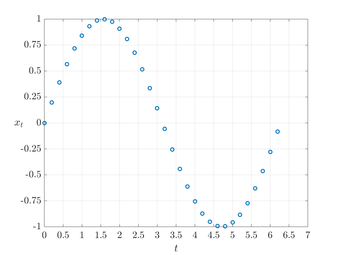

From snapshots of Figure 8, the KMD enables us to generate amplitude samples of size 6,284 () as Figure 10. We regard as the limiting distribution in Figure 11 by cubic spline interpolation. With the assumption of differentiability of with respect to , by taking partial derivatives, we approximate the governing probability as Figure 12.


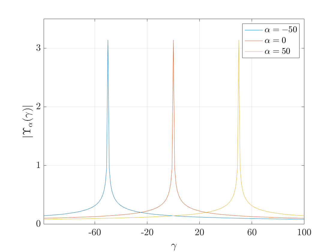
According to (25), every connection function of
is a translation of . Figure 13 shows three kinds of absolute values of . By (26), the learning rate of frequency with the sample regenerated is as follows,
Interpretation of estimations. Let be a dictionary of . Red dots of Figures 14 denote the active neurons for , , , and , respectively,
Active neurons have specific patterns formed by bundles of neighboring neurons. In pictures of Figure 14 we draw neighborhood groups of red areas of rectangles with rounded corners only on positive index set because of symmetry. As increases to , the adjacent groups of active neurons are distributed between frequencies and in of Figure 14. On the other hand, If is far from , the number of groups decreases, whereas the ball size increases. Moreover, if , then there is no such groups between and in of Figure 14.
In addition, we examine topological statistics on for , , , , and . In the union of -balls of each active path, the number of balls, mean, and variance of indexes are compared in Figures 15, 16, and 17, respectively.
Finally, from the network probability,
| (47) |
i.e., the likelihood has the maximum at the node and antinode. Hence, a random variable of amplitude for a standing wave has the maximum likelihood at peaks. With all , (47) and are identical. We can calculate likelihoods if the dictionary is main focus of interest.
Moment learning.
We derive the network probability for as a moment learning and analyze estimations of the network through the topological interpretation. Suppose that there are samples of drawn from (46) with time step for in Figure 18. By (36), the empirical distribution function is shown in Figure 19.
Using the KMD with , we gain 6,284 samples (Figure 20) with which we draw the limiting distribution and governing probability in Figures 21 and 22, respectively. Here, is calculated by partial derivatives of a finite-difference method at centers of equally spaced bins.
The sample has a uniform time step . By (28) the learning rate for moment is given by
According to topological statistics of Figures 15 17, mean- and variation-distributions have unstable behaviors on small balls when . Note that is the magnitude of an antinode. A loss of stem in figures is caused by absence of -ball in , and so, there does not exist any topological statistic at the position.
On the other hand, the induced is almost cylindrical and every partial derivative of vanishes at the origin. More precisely, is an approximation of singular measure which is supported in the unit circle and
Thus, does not belong to on . For this reason, the energy function cannot be expanded as a power series near the origin.
To avoid a dead end, we adopt an auxiliary function as a pullback limit of . Since could be regarded as the limit of suitable analytic functions, take an approximation of , for example,
| (48) |
where is chosen such that (see Figure 23). (In fact, the bowl-shaped functions such as have a similar distribution of neurons to Figures 24 27.)
Table I presents some examples of likelihoods of and with zero velocity. All express that has the maximum likelihood when .


More precisely,
and thus, we conclude that the likelihood of has the maximum when . In general, for , we obtain which have the maximum likelihood of . Therefore, is most likely in the network (refer to Figures 22 and 23). In fact, the relation between and is equal to for , e.g., when .


Interpretation of estimations. Let be a dictionary of indexes such that . The partial derivatives of at yield non-trivial neurons. For estimation and interpretation, we consider signals of , , , and , where double signs are in same order.
In Figures 24 and 27, we draw neurons and active paths induced from , in which red dots denote active paths for signals. For simplicity, we adopt -norm to generate the topology, with which we examine topological statistics on . For each , on the collection of all -balls, the number of balls, mean, and variance of indexes are compared in Figures 28, 29, and 30, respectively.
Note that all active paths do not contain any -ball for . In Figures 29 and 30, each position has values of two components. The right and left sides toward the distance increasing are the quantities from and , respectively.
There are plenty of mathematical research results for classification ([3, 7, 9, 12]). Those could be useful tools for interpreting unsupervised estimates.
Remark 9.1.
Without reproducing process of data, we could approximate the neurons of a probabilistic neural network. Indeed, the drawn sample would give the similar distribution of neurons to the probabilistic neural network. In many cases we do not need thousands or more of data to calculate neurons. However, the accuracy of the derived governing probability may be poor and the learning rate is low, because the accuracy depends on the sample size and quality.


10 Conclusion and Further study
The probabilistic neural network as an unsupervised learning model provides globally unique learning model as an optimal solution for observed samples in probability. The networks are essentially data driven models that do not depend on the back-propagation because our proposed networks are not trained through iterative computation. Hereby, these network models would be applied in a direction where quality is more important than amount of data in industry, e.g., such as financial service and bioengineering industries. These networks provide the learning rates which depend on the drawn samples, and thus, a probabilistic neural network maximizes the utilization of data. The application of probabilistic neural network technologies, especially for medical image classification, disease prediction, and object recognition, could provide accurate and reliable results.
To appreciate the estimation of artificial intelligence we may need certain physical interpretations and analysis of active neurons. For example, a suitable topology on the collection of all active paths or a dictionary containing a meaningful concept, e.g., the standard hearing range 20 to for humans, the -brainwave range 8 to , the first-order moments for (conditional) expectations, etc.
References
- [1] H. Arbabi and I. Mezić. Ergodic theory, dynamic mode decomposition, and computation of spectral properties of the Koopman operator. SIAM J. Appl. Dyn. Syst. 16(4), 2096–2126, 2017.
- [2] Y. Bengio, A. Courville, and P. Vincent. Representation learning: A review and new perspectives. IEEE Trans.Pattern Anal. Machine Intelli. (35), pp. 1798–1828, 2013.
- [3] C. M. Bishop. Pattern recognition and machine learning. Springer, 2006.
- [4] G. Cybenko. Approximation by superpositions of a sigmoidal function. Mathematics of Control, Signals and Systems 2, pp. 303–314, 1989
- [5] S. Furaoa and O. Hasegawa. An incremental network for on-line unsupervised classification and topology learning. Neural Networks 19, 90–106, 2006.
- [6] R. Geirhos, D. H. J. Janssen, H. H. Schütt, J. Rauber, M. Bethge, F. A. Wichmann. Comparing deep neural networks against humans: object recognition when the signal gets weaker. ArXiv abs/1706.06969, 2017
- [7] I. Goodfellow, Y. Bengio and A. Courville. Deep learning. MIT Press, 2016.
- [8] L. Grafakos. Classical and modern Fourier Analysis Prentice Hall, 2003.
- [9] S. Haykin. Neural networks and learning machines. Pearson, 2016.
- [10] K. Hornik. Approximation capabilities of multilayer feedforward networks. Neural Networks 4(2), pp. 251–257, 1991.
- [11] M. Korda and I. Mezić. On convergence of extended dynamic mode decomposition to the Koopman operator. Jour. Nonlinear Science 28, pp. 687–710, 2018.
- [12] K. P. Murphy. Machine learning: A probabilistic perspective (Adaptive Computation and Machine Learning series). The MIT Press, 2012.
- [13] C. W. Rowley, I. Mezić, S. Bagheri, P. Schlatter, and D. S. Henningson. Spectral analysis of nonlinear flows. Jour. Fluid Mech. 641, pp. 115–127, 2009.
- [14] P. Schmid. Dynamic mode decomposition of numerical and experimental data. Jour. Fluid Mech. 656, pp. 5–28, 2010.
- [15] P. Schmid and J. Sesterhenn. Dynamic mode decomposition of numerical and experimental data. American Physical Society, 61st Annual Meeting of the APS Division of Fluid Dynamics, November 23–25, 2008, abstract id. MR.007.
- [16] G. R. Shorack and J. A. Wellner. Empirical processes with applications to statistics. John Wiley & Sons, Inc., 1986.
- [17] E. M. Stein. Harmonic Analysis: Real-variable methods, orthogonality, and oscillatory Integrals, Princeton University Press, 1993.
- [18] J. H. Tu, C. W. Rowley, D. M. Luchtenburg, S. L. Brunton, and J. N. Kutz. On dynamic mode decomposition: Theory and applications. Jour. Comp. Dynamics 1(2), pp. 391–421, 2014.
- [19] D. Watson. The rhetoric and reality of anthropomorphism in artificial intelligence. Minds and Machines 29, pp. 417–440, 2019.
![[Uncaptioned image]](2004.10745v1/MATLAB/ksrim.png) |
Kyung Soo Rim received the B. S. degree from Korea University (KU), Korea in 1990, the MS and Ph. D. degree in harmonic analysis of mathematics from Korea Advanced Institute of Science and Technology (KAIST), Korea in 1992 and 1996, respectively. He is a full professor in the department of mathematics at Sogang University in Seoul, Korea and served as the Dean of Academic and Admissions Affairs from 2015-18. His recent research interests focus on the probabilistic machine intelligence related to the Koopman operator of dynamical systems including the continuity of convolution and compositions between function spaces. |
![[Uncaptioned image]](2004.10745v1/MATLAB/ujchoi.png) |
U Jin Choi received the B. S. degree from Seoul National University (SNU), Korea in 1974 and Ph. D. degree from Carnegie Mellon University in 1987, U. S. A., both in mathematics. He is currently emeritus professor at Korea Advanced Institute of Science and Technology (KAIST) and a member of Research Advisory Committee at National Institute of Mathematical Sciences (NIMS), Korea and served as a full professor in the department of mathematical sciences at KAIST until 2011. His current research interests are statistics, dynamical systems theory, and machine intelligence in viewpoint of mathematics including stochastic calculus. |