Sato-Tate Distributions of and
Abstract.
We determine the Sato-Tate groups and prove the generalized Sato-Tate conjecture for the Jacobians of curves of the form and where is an odd prime. Our results rely on the fact the Jacobians of these curves are nondegenerate, a fact that we prove in the paper. Furthermore, we compute moment statistics associated to the Sato-Tate groups. These moment statistics can be used to verify the equidistribution statement of the generalized Sato-Tate conjecture by comparing them to moment statistics obtained for the traces in the normalized -polynomials of the curves.
Key words and phrases:
Sato-Tate groups, Sato-Tate distributions, Hyperelliptic curves2010 Mathematics Subject Classification
11M50, 11G10, 11G20, 14G101. Introduction
The original Sato-Tate conjecture is a statistical conjecture regarding the distribution of the normalized traces of Frobenius on an elliptic curve without complex multiplication (CM), and the conjecture was recently generalized to higher genus curves by Serre [31]. Recent results on this topic of determining Sato-Tate distributions in genus 2 and 3 curves have been achieved in [3, 12, 13, 14, 15, 16, 23, 26]. In 2016, Fité-González-Lario [11] obtained Sato-Tate equidistribution results for a family of curves of arbitrarily high genus. The main purposes of this paper are to compute the Sato-Tate groups and to prove the generalized Sato-Tate conjecture for the following two families of hyperelliptic curves of arbitrarily high genus
where is an odd prime. The generalized Sato-Tate conjecture is known for CM abelian varieties due to the work of Johansson in [22]; in our proof for we follow Serre’s strategy from [30]. We provide numerical evidence to support our results by computing moment statistics associated to the curves.
We start by recalling the original Sato-Tate conjecture for elliptic curves. Let be a number field, be an elliptic curve without complex multiplication, and be a finite prime of such that has good reduction at . By a theorem of Hasse, the number of points of is , where denotes the residue field of and is an integer (called the trace of Frobenius at ) satisfying . The Sato-Tate conjecture predicts that, as varies through the primes of good reduction for , the normalized Frobenius traces are equidistributed in the interval with respect to the image of the Haar measure on the special unitary group . This conjecture has been proven for non-CM elliptic curves defined over totally real fields (see [6, 7, 17, 36]). The distributions of the normalized Frobenius traces are also known for CM elliptic curves over all fields: they are distributed with respect to the image under the trace map of the Haar measure on either the unitary group or the normalizer of in , depending on whether or not the field of definition contains the field of complex multiplication (see, for example, [1] or [5]).
The generalized Sato-Tate conjecture for an abelian variety predicts the existence of a compact Lie group that determines the limiting distribution of normalized local Euler factors. We now state the conjecture more precisely for abelian varieties that are the Jacobians of curves defined over , following the exposition of [11].
Let be a smooth, projective, genus curve defined over and let be the minimal extension over which all endomorphisms of are defined. The Sato-Tate group of the Jacobian of , , is a compact Lie group satisfying the following property. For each prime at which has good reduction, there exists a conjugacy class of whose characteristic polynomial equals the normalized -polynomial
| (1) |
Let be a number field and let be the set of conjugacy classes of . Let be an ordering by norm of the set of primes of good reduction for over and define a map that sends to in . We can now state the generalized Sato-Tate conjecture.
Conjecture 1.1.
(Generalized Sato-Tate Conjecture) The sequence is equidistributed on with respect to the image on of the Haar measure of
Our goals in this paper are to determine the Sato-Tate groups of the Jacobians of the curves and (see Theorem 4.2 and Theorem 4.4) and to prove the equidistribution predicted by the generalized Sato-Tate conjecture for these two families of curves (see Theorem 5.5 and Theorem 5.6).
Theorem 1.2.
Let be an odd prime. The generalized Sato-Tate conjecture holds for the Jacobians of the curves and .
The Sato-Tate conjecture was proven for CM abelian varieties in [22], and the Jacobians of both curves in Theorem 1.2 are CM abelian varieties. However, to provide an explicit description of the limiting distribution of the normalized -polynomial, we need the explicit embedding of the Sato-Tate group of the Jacobian of the curve inside , where is the genus of the curve. Our approach is similar to that of, for example, [11] and [26].
This paper is organized as follows. In Section 2, we establish the nondegeneracy of the Jacobians of and . In Section 3, we prove that the twisted Lefschetz group of the Jacobian, defined by Banaszak and Kedlaya in [5], is equal to the algebraic Sato-Tate group; this essentially follows from the work of [4] since the Jacobians of our curves are nondegenerate. The equality of the twisted Lefschetz group and the algebraic Sato-Tate group allows one to interpret the Sato-Tate group as a maximal compact subgroup of the group of -points of the base change of the algebraic Sato-Tate group to .
In Section 4, we apply the work of Section 3 to determine the Sato-Tate groups of the Jacobians of the curves and . We first determine the identity components of the Sato-Tate groups (see Proposition 4.1 and Proposition 4.3). Note that these propositions confirm Conjectures 6.8 and 6.9 of [9]. The computation of the twisted Lefschetz groups then gives the generators of the component groups (see Theorems 4.2 and 4.4). We give explicit examples of some of these generators in Table 3 in Appendix A.
In Section 5, we establish Conjecture 1.1 for and . For the curve , we prove the generalized Sato-Tate conjecture by following Serre’s strategy in [30], i.e. showing that a certain -function attached to the irreducible nontrivial representations of the Sato-Tate group of the Jacobian of the curve does not vanish. We then use a theorem of Hecke that the -function attached to a nontrivial unitarized Hecke character does not vanish for Re This proof technique requires a cyclic Galois group , where is the minimal extension over which all endomorphisms of the Jacobian are defined. The Galois group associated to the curve is not cyclic, so we use the work of [22] to prove the generalized Sato-Tate conjecture in this case.
In Section 6, we compute moment statistics associated to the Sato-Tate groups of the Jacobians of and . These moment statistics can be used to verify the equidistribution statement of the generalized Sato-Tate conjecture by comparing them to moment statistics obtained for the traces in the normalized -polynomial in Equation (1). Note that the numerical moment statistics are an approximation since one can only ever compute them up to some prime. It is of interest to those dealing with equidistribution statements to compare how close these two computations are. We compare the moments in Table 2 in Section 6.
Notation and conventions
We begin by fixing notation used in later sections. Let be a smooth projective curve defined over . We write for the ring of endomorphisms defined over the field of the Jacobian of . Let denote the minimal extension over which all the endomorphisms of the abelian variety are defined, i.e. the minimal extension for which ; the field is called the endomorphism field of .
We denote the Sato-Tate group of the Jacobian of by with identity component denoted and component group . The curve is denoted by , and when we specialize to or to we assume throughout the paper that is an odd prime. We will write for a primitive root of unity. For any rational number whose denominator is coprime to an integer , denotes the unique representative of modulo between 0 and .
Define the two matrices
The symplectic form considered throughout the paper is given by Lastly, for any positive integer , we define the following subgroups of the unitary symplectic group .
and
Acknowledgements
This material is based upon work supported by the National Security Agency under Grant No. H98230-19-1-0119, The Lyda Hill Foundation, The McGovern Foundation, and Microsoft Research, while the authors were in residence at the Mathematical Sciences Research Institute in Berkeley, California, during the summer of 2019. The first named author was supported by NSF grant DMS-2002085 and an AMS-Simons Travel Award. The second author also received support for this project provided by a PSC-CUNY Award, jointly funded by The Professional Staff Congress and The City University of New York.
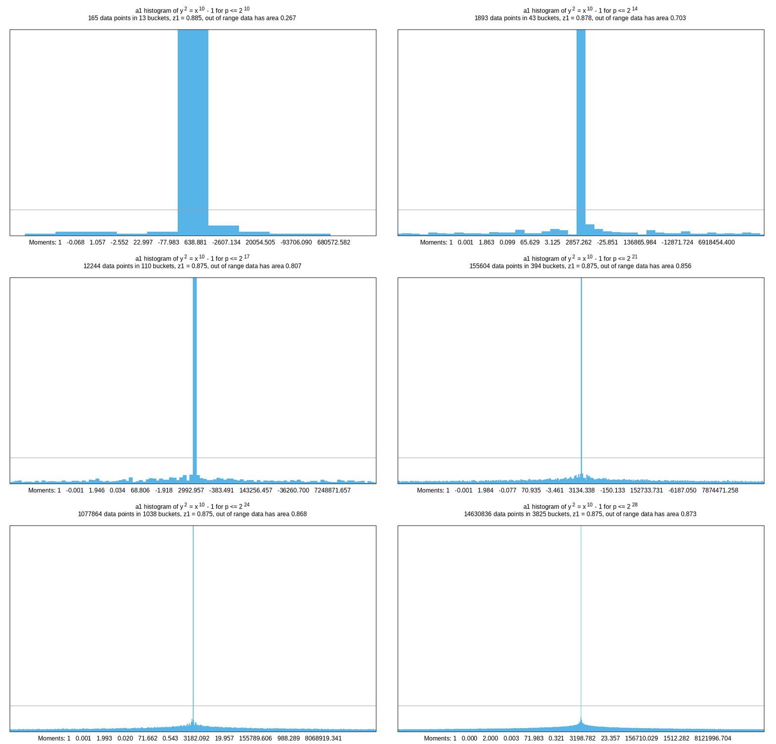
We would like to thank Francesc Fité for enlightening discussions while working on this project and Drew Sutherland for creating the histogram in Figure 1 for us (see also [34]). We also thank Christelle Vincent, Holley Friedlander, and Fatma Cicek for their help with the Sage code to compute the matrices and the characteristic polynomials during Sage Days 103. Lastly, we thank the reviewer for their thorough and helpful comments.
2. Nondegenerate Abelian Varieties
Our main results hold for curves whose Jacobians are nondegenerate. In this section we define the term nondegenerate and give some known results that will be relevant to our later work.
Let be a nonsingular projective variety over . We denote (as in [33]) the (complexified) Hodge ring of by
where is the -span of Hodge cycles of codimension on . Furthermore, we define the ring
where is the -span of classes of intersection of divisors. This is the subring of generated by the divisor classes, i.e. generated by . In general, it is known that we have containment [33].
Definition 2.1.
[2] An abelian variety is said to be nondegenerate if . If , then is said to be degenerate.
Definition 2.2.
Hazama proves in Theorem 1.2 of [20] that is stably nondegenerate if and only if the dimension of its Hodge group is maximal. Note that in [11], the authors use the word nondegenerate to describe abelian varieties with this property.
Nondegeneracy is related to the CM-type of an abelian variety. Let be a dimension abelian variety. Suppose that there is a number field with and an injective ring homomorphism . The map induces a representation of on the space of holomorphic 1-forms on and we say that is of CM-type (see, for example, [32, 24, 2, 28]). When is an absolutely simple abelian variety with complex multiplication, stable nondegeneracy is equivalent to the CM-type being nondegenerate, i.e. the CM-type has maximal rank (see, for example, [24, 2]).
Let be the subspace of generated by the classes of algebraic cycles on of codimension . Then
and the Hodge Conjecture for asserts that for all [2, 33]. It is clear from Definition 2.1 that if is nondegenerate then the Hodge Conjecture holds. However, there are many cases where the Hodge Conjecture holds for degenerate abelian varieties. For example, Shioda verified the Hodge Conjecture for for all , though , , and are degenerate (see [33, Section 6]).
The following results are crucial to our work with the curves and .
Proposition 2.3.
[33, Corollary 5.3] If is a prime number, then the Hodge ring is generated by . The same result holds for arbitrary powers of .
By definition, this tells us that is stably nondegenerate. The nondegenerate CM-type for the curve is , where each is defined by (see, for example, [32, Section 15.4]). The CM-type for the curve is primitive (see, for example, [24] for a definition) which implies that is absolutely irreducible.
Proposition 2.4.
[9, Lemma 4.1] Let be an even integer, and , where . Then we have the following isogeny over
where .
Combining these two results yields the following.
Corollary 2.5.
For any prime , and are nondegenerate.
Proof.
3. The Algebraic Sato-Tate Group
We start by defining notation as in [11] and [35, Section 3]. For more detailed background information, see [35, Section 3.2].
Let be an abelian variety of dimension defined over the number field . Let be a prime and we define the Tate module to be a free -module of rank , and the rational Tate module to be a -vector space of dimension The Galois action on the Tate module is given by an -adic representation
Let denote the image of this map, and let be the Zariski closure of in . We then define .
Definition 3.1.
The Sato-Tate group of , denoted by , is a maximal compact Lie subgroup of contained in
The algebraic Sato-Tate Conjecture for predicts the existence of an algebraic Sato-Tate group of such that
for every prime (see, for example, [12, Conjecture 2.13] and [5, Conjecture 2.1]).
For each , define the set
where is viewed as an endomorphism of
Definition 3.2.
[5] The twisted Lefschetz group is defined to be
When is the identity automorphism, forms a group, called the Lefschetz group, which we denote simply by .
Proposition 3.3.
Let be an odd prime and be the curve . Then the algebraic Sato-Tate Conjecture holds for with .
Proof.
This follows from [5, Theorem 6.6] since is a nondegenerate CM abelian variety. Still, we include a proof that is similar to the proof of [11, Lemma 3.5] for the sake of completion. By [12, Theorem 2.16(a)], we need to verify two criteria: the Hodge group equals the Lefschetz group , and that the Mumford-Tate Conjecture holds for . The Mumford-Tate Conjecture is known to be true for CM abelian varieties (see, for example, [11, 28, 39]), so we only need to verify the first of the criteria.
By Deligne [8, I, Proposition 6.2] and [5, Definition 4.4], we have
| (2) |
for every prime . We will show that to obtain the desired result. Note that it is sufficient to show this for any prime .
Since is prime, is simple (see, for example, [32, Section 15.4]). Furthermore, Proposition 2.3 tells us that has nondegenerate CM-type. We apply the results of Section 2 of [4] to get, for every prime of good reduction for which splits completely in ,
| (3) |
where is the genus of .
We now compute the Lefschetz group . In order for a matrix to commute with any matrix , it must be diagonal. Hence,
which yields the desired result. ∎
Corollary 3.4.
If is an odd prime then the algebraic Sato-Tate Conjecture holds for with .
Proof.
Note that we cannot apply Theorem A of [4] to determine since is not simple. We will determine the identity component of the Sato-Tate group of using another method in Section 4.2.
Corollary 3.5.
The group of components of and are isomorphic to . Also, the group of components of and are isomorphic to .
Remark.
It is known that when the algebraic Sato-Tate conjecture holds, we may interpret the Sato-Tate group as a maximal compact subgroup of (see, for example, [12, Section 2.2]).
4. Sato-Tate Groups
In this section we compute the Sato-Tate groups of the Jacobians of the curves and . For both families of curves, we obtain the component group of the Sato-Tate group by computing the twisted Lefschetz groups (recall the results of Proposition 3.3 and Corollary 3.4).
4.1. The Sato-Tate Group of
We first determine the identity component of the Sato-Tate group.
Proposition 4.1.
If is an odd prime then
where is the genus of .
Proof.
Remark.
The main result of the following theorem is determining the component group of the Sato-Tate group of . Explicit examples of the generator of the component group are given in Table 3 in Appendix A.
Theorem 4.2.
Let and let be a generator of the cyclic group . Up to conjugation in ,
where is a matrix whose block entries are given by
| (4) |
Furthermore, there is an isomorphism
Proof.
We compute the twisted Lefschetz group of . Applying Proposition 3.3 then yields the desired result.
We can identify the group with via the isomorphism that maps to the Galois element ,where .
A basis for the space of regular -forms of a genus hyperelliptic curve is given by (see, for example, [37, Section 3]). We consider the automorphism defined by , and compute the pullbacks of the differentials to be
We now write the endomorphism in terms of a symplectic basis of (with respect to the matrix ) and get the diagonal matrix where each is a block matrix defined by
Let be a generator for the cyclic Galois group . Since the action of the Galois element is given by , we have
Hence, letting , we can write
where
Note that . This characterization allows to express each in the form or , for some .
We will now verify that , where is as defined in Equation (4). Note that there is only one nonzero block entry in each row and each column in the block matrix . Furthermore, one easily checks that the entries of the inverse of are given by
Some basic linear algebra shows that the only nonzero blocks in the product will be the diagonal entries. We will now determine what those diagonal entries will be. Suppose that the only nonzero block in column of is in row . Based on the definitions of and , this nonzero entry will yield the following product in the th diagonal entry of
Hence, , which confirms that is an element of the twisted Lefschetz group.
We now show that , but for any proper divisor of , which will prove that
Since generates the Galois group , we have and, for ,
and nor otherwise. Hence, the action of on the block matrix satisfies
for some not equal to .
We have seen that , and so conjugating by permutes (and sometimes conjugates) the diagonal block entries of . Since is again a diagonal block matrix, conjugating this by will again just permute (and sometimes conjugate) the diagonal block entries. Hence, is a diagonal block matrix for any . In fact, we can write .
Thus, has a nonzero, off-diagonal block entry if and only if there is some for which or with . This is possible if and only if or .
If , then for all . Hence, all of the diagonal block entries of must be or since . Thus, . However, , so , which is an element of . Thus,
∎
4.2. The Sato-Tate Group of
We use the results of Section 2 and Proposition 4.1 to determine the identity component of the Sato-Tate group of .
Proposition 4.3.
If is an odd prime and , then
where is the genus of .
Proof.
The main result of the following theorem is determining the component group of the Sato-Tate group of . This is an interesting addition to the literature as the Sato-Tate groups of these curves do not have cyclic component groups.
Theorem 4.4.
Let be an odd prime, , , and be a generator of the cyclic group . Up to conjugation in , the Sato-Tate group of is
where the block entries of are given by
for , and Furthermore, there is an isomorphism
Proof.
The reduced automorphism group of is isomorphic to the dihedral group (see, for example, [27]). We consider the following generators of the automorphism group of . Let
where is a primitive root of unity. Thus, , where .
We compute pullbacks of the differentials , where , in order to determine the generators of the endomorphism ring . As in the proof of Theorem 4.2, the pullback leads to the endomorphism . Computing the pullback on the differential yields
Thus, the endomorphism is the antidiagonal matrix , where
We choose two elements that generate the Galois group and satisfy
where is a generator of .
Let and be defined as in the statement of the theorem. One can verify that
using a similar strategy to the one used in the proof Theorem 4.2, so we omit the proof here. In this case, the matrix contains both and as entries so that it conjugates properly.
Lastly, one can show as in the proof of Theorem 4.2 that the component group of is .
∎
Corollary 4.5.
Up to conjugation in , the Sato-Tate group of over is
Proof.
This follows from the fact that the minimal extension over which all the endomorphisms of are defined is . ∎
5. Equidistribution Results
In this section we prove Theorem 1.2, which states that the generalized Sato-Tate conjecture holds for the Jacobians of and . We first specify to the curve . We begin by discussing the -functions associated to the curve and then state the generalized Sato-Tate conjecture. We then prove the generalized Sato-Tate conjecture following the strategy of Serre [30]. Finally, we prove the generalized Sato-Tate conjecture for the Jacobian of using a result of [22].
5.1. Hecke Characters and -Functions
We follow the exposition in [11, Section 2.2], specifying to the curve . For a more thorough review of Hecke characters, we refer the reader to [25] and [38]. Let be a prime ideal to in and let be an element in the ring of integers of . Then there is precisely one root of unity satisfying the condition
We extend this to all of by setting whenever , and, thus, is a multiplicative character of order on .
We now define the Jacobi sums that appear in the -functions of our curves. For all , and for any ideal in not dividing , we define
(see [25, Section 1.4]) and can be viewed as a function on in terms of the characters on (see [38]). For each we extend the definition of to all ideals prime to in by multiplicativity.
Lemma 5.1.
Let be of the form for then
5.2. Generalized Sato-Tate Conjecture
We specify the generalized Sato-Tate conjecture to the Jacobian of the curve . Before we state the conjecture, we need to set up some notation.
Let be a subextension of . Denote the set of conjugacy classes of by . Let be an infinite subset of primes of a number field, and be an ordering by norm of . Define a map by sending to . For any representation of , write
We specify a theorem of Serre to the curve (see also [11, Theorem 3.12]).
Theorem 5.2.
[30, page I-23] Suppose that for every irreducible nontrivial representation of the Euler product converges for Re and extends to a holomorphic and nonvanishing function for Re. Then the sequence is equidistributed over with respect to the projection on of the Haar measure of .
For a prime of , let be the conjugacy class of using the isomorphism . Specifically, set
where each . The set is a complete set of representatives of , and is a prime of lying over .
Now specify to be the set of primes of good reduction for and let be an ordering by norm of . We can now state the generalized Sato-Tate conjecture for (see, for example, [30, page I-23]).
Conjecture 5.3 (Generalized Sato-Tate).
The sequence is equidistributed on with respect to the image on of the Haar measure of
The following theorem specifies this conjecture to .
Theorem 5.4.
The generalized Sato-Tate conjecture holds for over .
Proof.
See [10, Theorem 3.6]. ∎
To prove Conjecture 5.3 for over , we will prove the convergence condition of Theorem 5.2. We first describe the irreducible representations of as in [29]. Let so that . We associate to any tuple the irreducible representation defined by
where
Let be the subgroup such that
| (5) |
for every . Let Then we can extend to via the map
By work of Serre [29], every irreducible representation of is of the form , where is a character of viewed as a character of using composition with the projection .
Theorem 5.5.
The generalized Sato-Tate conjecture holds for over .
Proof.
Let be the cardinality of . We first consider the case where is the trivial character. The theory of -functions gives
Note that the second equality holds by Equation (5). By [10, Section 3.5], we then have up to a finite number of Euler factors, where is a Grössencharacter and is holomorphic and nonvanishing on Re.
We now consider the case where is non-trivial. Since is cyclic there exists a character of such that restricted to equals Thus,
Furthermore, being cyclic also gives us that
Hence, we again have that up to a finite number of Euler factors, where is a Grössencharacter and is holomorphic and nonvanishing on Re. ∎
Remark.
The result also follows from [22, Prop. 16].
Theorem 5.6.
Let be any subextension of . Then the generalized Sato-Tate conjecture holds for over .
6. Moment Statistics
In this Section we compute moment statistics associated to the Sato-Tate groups. These moment statistics can be used to verify the equidistribution statement of the generalized Sato-Tate conjecture by comparing them to moment statistics obtained for the traces in the normalized -polynomial in Equation (1).
6.1. Preliminaries
The following background information has been adapted from [26, Section 4] and [35, Section 4]. We start by recalling some basic properties of moment statistics. We define the th moment (centered at 0) of a probability density function to be the expected value of the th power of the values, i.e. .
Recall that for independent variables and we have and (see, for example, [26]). Thus, we have the following
| (6) |
| (7) |
and
| (8) |
Furthermore, for any constant , we have .
We will now work to define the Haar measure on the groups that we obtain for the identity component . From Propositions 4.1 and 4.3 we see that the possible groups are
For each of these groups, we are interested in the pushforward of the Haar measure onto the set of conjugacy classes conj() or conj().
We start with the unitary group and consider the trace map on defined by , where . This trace map takes values in . From here we see that and
gives a uniform measure of on (see [35, Section 2]). We can deduce the following pushforward measures
Note that though the measure is expressed the same as the measure , we will get a different distribution since in the former case each eigenangle occurs with multiplicity 2 (see, for example, [35, Section 4.3]).
We can now define the moment sequence , where is a positive measure on some interval . The moment is, by definition, the expected value of with respect to , where is the function . It is therefore given by
For we have , where if is odd. Hence,
From here, we can compute , and take binomial convolutions to obtain
We can combine these strategies with Equations (6), (7), and (8) to compute moments for and .
For each , denote by the projection of the Haar measure onto the interval We can compute by averaging over the components of the Sato-Tate group. For example, in the case where the curve has CM by , we will denote the restriction of to the component by and
6.2. Characteristic Polynomials
In this subsection, we give results for the characteristic polynomials in each component of the Sato-Tate groups of and .
6.2.1. Characteristic Polynomials for
We start with a random matrix in the identity component . We will denote the characteristic polynomial of by . Since , we only compute for .
Example 6.1.
We compute the characteristic polynomials of the curve . This yields and
We have two general results for the characteristic polynomials associated to the Sato-Tate group of , which we combine into the following proposition.
Proposition 6.2.
Let be the genus curve , where is prime. Then
Proof.
The first equality is a consequence of Proposition 4.1 which tells us that .
For a justification of the second equality, we recall from our work in the proof of Theorem 4.2. There we proved that is a diagonal block matrix with on its diagonal entries. Multiplying by yields a diagonal block matrix, whose diagonal blocks are of the form
depending on whether we multiplied by or . In either case, the factor of the characteristic polynomial associated to this block is of the form
Thus, since there are diagonal blocks, the characteristic polynomial is
∎
6.2.2. Characteristic Polynomials for
We again start with a random matrix in the identity component of the Sato-Tate group. Recall that the Sato-Tate group of has two generators for the component group: and . We will denote the characteristic polynomial of by . Since , we only compute for and .
Example 6.3.
We compute the characteristic polynomials of the curve . This yields and
We have two general results for the characteristic polynomials associated to the Sato-Tate group of , which we combine into the following proposition.
Proposition 6.4.
Let be the genus curve , where is prime. Then
Proof.
We also have the following conjecture.
Conjecture 6.5.
Let be the genus curve , where is prime. Then for any relatively prime to and or 1.
6.3. General Results for the Moments
Based on the results of Section 6.2.1, we have the following general result for the moment statistics associated to the Sato-Tate group of .
Proposition 6.6.
For the curve we have
Proof.
Recall from Proposition 6.2 that Expanding this yields
Thus, when is even and it equals 0 when is odd. It is then clear that in this case is when is even and 0 when is odd ∎
We also have the following conjecture for characteristic polynomials and moments.
Conjecture 6.7.
Let be the genus curve , where is prime. Then for any relatively prime to and .
6.4. Explicit Examples of Moment Statistics
We first determine moment statistics for the genus 5 curve . Using characteristic polynomials that were computed for each component in Example 6.1 and the properties in Equations (6), (7), and (8), we can compute the th moments for each , . These moments, given in Table 1, are easily computed using Sage [21]. See Table 2 in Section 6.5 for a comparison of to the numerical moments of the normalized -polynomial of the curve.
Using the same strategy as above, we determine that the -moment statistics for the Sato-Tate group of are
In Figure 1 we give a histogram of -values of , as well as moment statistics (up to the 10th moment). Observe that the numerical moments , which are computed using primes up to , are quite close to what we obtained for . See [34] for an animated histogram of the -distribution. The algorithm used to make the histogram is described in [18] and [19].

See Table 2 in Section 6.5 for moment statistics for other curves.
6.5. Tables of - and -Moment Statistics
We first consider curves of the form . Note that for all . One can easily determine from Proposition 6.2 that the coefficient of in is , where . Hence,
| (9) |
Similarly, for curves of the form ,
| (10) |
whenever and otherwise.
We used Sage [21] to evaluate Equations (9) and (10), and then average over the components, to get the -moments shown in Table 2. Note that for all odd , so we omit those values from the table. For comparison, we computed the numerical -moments for primes up to .
| 10 | 2 | 72 | 3200 | 156800 | |
|---|---|---|---|---|---|
| 11 | 1 | 27 | 1090 | 55195 | |
| 13 | 1 | 33 | 1660 | 106785 | |
| 14 | 2 | 120 | 9920 | 954240 | |
| 17 | 1 | 45 | 3160 | 290605 | |
| 19 | 1 | 51 | 4090 | 432915 | |
| 22 | 2 | 216 | 34880 | 7064960 | |
Appendix A Examples of the Matrix
In Table 3 we give examples of the matrix from Theorems 4.2 and 4.4. These were computed in Sage [21] using Sage’s chosen generators for and .
| 10 | 13 | ||
|---|---|---|---|
| 11 | 14 |
References
- [1] P. B. Allen, F. Calegari, A. Caraiani, T. Gee, D. Helm, B. V. L. Hung, J. Newton, P. Scholze, R. Taylor, and J. A. Thorne. Potential automorphy over cm fields, 2018.
- [2] N. Aoki. Hodge cycles on CM abelian varieties of Fermat type. Comment. Math. Univ. St. Paul., 51(1):99–130, 2002.
- [3] S. Arora, V. Cantoral-Farfán, A. Landesman, D. Lombardo, and J. S. Morrow. The twisting Sato-Tate group of the curve . Math. Z., 290(3-4):991–1022, 2018.
- [4] G. Banaszak, W. Gajda, and P. Krasoń. On Galois representations for abelian varieties with complex and real multiplications. J. Number Theory, 100(1):117–132, 2003.
- [5] G. Banaszak and K. S. Kedlaya. An algebraic Sato-Tate group and Sato-Tate conjecture. Indiana Univ. Math. J., 64(1):245–274, 2015.
- [6] T. Barnet-Lamb, D. Geraghty, M. Harris, and R. Taylor. A family of Calabi-Yau varieties and potential automorphy II. Publ. Res. Inst. Math. Sci., 47(1):29–98, 2011.
- [7] L. Clozel, M. Harris, and R. Taylor. Automorphy for some -adic lifts of automorphic mod Galois representations. Publ. Math. Inst. Hautes Études Sci., (108):1–181, 2008. With Appendix A, summarizing unpublished work of Russ Mann, and Appendix B by Marie-France Vignéras.
- [8] P. Deligne, J. S. Milne, A. Ogus, and K.-y. Shih. Hodge cycles, motives, and Shimura varieties, volume 900 of Lecture Notes in Mathematics. Springer-Verlag, Berlin-New York, 1982.
- [9] M. Emory, H. Goodson, and A. Peyrot. Towards the Sato-Tate groups of trinomial hyperelliptic curves. Int. J. Number Theory, 17(10):2175–2206, 2021.
- [10] F. Fité. Equidistribution, -functions, and Sato-Tate groups. In Trends in number theory, volume 649 of Contemp. Math., pages 63–88. Amer. Math. Soc., Providence, RI, 2015.
- [11] F. Fité, J. González, and J.-C. Lario. Frobenius distribution for quotients of Fermat curves of prime exponent. Canad. J. Math., 68(2):361–394, 2016.
- [12] F. Fité, K. S. Kedlaya, V. Rotger, and A. V. Sutherland. Sato-Tate distributions and Galois endomorphism modules in genus 2. Compos. Math., 148(5):1390–1442, 2012.
- [13] F. Fité, K. S. Kedlaya, and A. V. Sutherland. Sato-Tate groups of abelian threefolds: a preview of the classification. ArXiv e-prints, page arXiv:1911.02071, Nov. 2019.
- [14] F. Fité, E. Lorenzo García, and A. V. Sutherland. Sato-Tate distributions of twists of the Fermat and the Klein quartics. Res. Math. Sci., 5(4):Paper No. 41, 40, 2018.
- [15] F. Fité and A. V. Sutherland. Sato-Tate distributions of twists of and . Algebra Number Theory, 8(3):543–585, 2014.
- [16] F. Fité and A. V. Sutherland. Sato-Tate groups of and . In Frobenius distributions: Lang-Trotter and Sato-Tate conjectures, volume 663 of Contemp. Math., pages 103–126. Amer. Math. Soc., Providence, RI, 2016.
- [17] M. Harris, N. Shepherd-Barron, and R. Taylor. A family of Calabi-Yau varieties and potential automorphy. Ann. of Math. (2), 171(2):779–813, 2010.
- [18] D. Harvey and A. V. Sutherland. Computing Hasse-Witt matrices of hyperelliptic curves in average polynomial time. LMS J. Comput. Math., 17(suppl. A):257–273, 2014.
- [19] D. Harvey and A. V. Sutherland. Computing Hasse-Witt matrices of hyperelliptic curves in average polynomial time, II. In Frobenius distributions: Lang-Trotter and Sato-Tate conjectures, volume 663 of Contemp. Math., pages 127–147. Amer. Math. Soc., Providence, RI, 2016.
- [20] F. Hazama. Algebraic cycles on nonsimple abelian varieties. Duke Math. J., 58(1):31–37, 1989.
- [21] S. Inc. CoCalc Collaborative Computation Online, 2020. https://cocalc.com/.
- [22] C. Johansson. On the Sato-Tate conjecture for non-generic abelian surfaces. Trans. Amer. Math. Soc., 369(9):6303–6325, 2017. With an appendix by Francesc Fité.
- [23] K. S. Kedlaya and A. V. Sutherland. Hyperelliptic curves, -polynomials, and random matrices. In Arithmetic, geometry, cryptography and coding theory, volume 487 of Contemp. Math., pages 119–162. Amer. Math. Soc., Providence, RI, 2009.
- [24] T. Kubota. On the field extension by complex multiplication. Trans. Amer. Math. Soc., 118:113–122, 1965.
- [25] S. Lang. Cyclotomic fields I and II, volume 121 of Graduate Texts in Mathematics. Springer-Verlag, New York, second edition, 1990. With an appendix by Karl Rubin.
- [26] J.-C. Lario and A. Somoza. The Sato-Tate conjecture for a Picard curve with complex multiplication (with an appendix by Francesc Fité). In Number theory related to modular curves—Momose memorial volume, volume 701 of Contemp. Math., pages 151–165. Amer. Math. Soc., Providence, RI, 2018.
- [27] N. Müller and R. Pink. Hyperelliptic Curves with Many Automorphisms. arXiv e-prints, page arXiv:1711.06599, Nov 2017.
- [28] H. Pohlmann. Algebraic cycles on abelian varieties of complex multiplication type. Ann. of Math. (2), 88:161–180, 1968.
- [29] J.-P. Serre. Linear representations of finite groups. Springer-Verlag, New York-Heidelberg, 1977. Translated from the second French edition by Leonard L. Scott, Graduate Texts in Mathematics, Vol. 42.
- [30] J.-P. Serre. Abelian -adic representations and elliptic curves, volume 7 of Research Notes in Mathematics. A K Peters, Ltd., Wellesley, MA, 1998. With the collaboration of Willem Kuyk and John Labute, Revised reprint of the 1968 original.
- [31] J.-P. Serre. Lectures on , volume 11 of Chapman & Hall/CRC Research Notes in Mathematics. CRC Press, Boca Raton, FL, 2012.
- [32] G. Shimura and Y. Taniyama. Complex multiplication of abelian varieties and its applications to number theory, volume 6 of Publications of the Mathematical Society of Japan. The Mathematical Society of Japan, Tokyo, 1961.
- [33] T. Shioda. Algebraic cycles on abelian varieties of Fermat type. Math. Ann., 258(1):65–80, 1981/82.
- [34] A. V. Sutherland. Sato-tate distribution of . http://math.mit.edu/~drew/x10m1_a1f.gif, 2019. Accessed: 2019-09-10.
- [35] A. V. Sutherland. Sato-Tate distributions. In Analytic methods in arithmetic geometry, volume 740 of Contemp. Math., pages 197–248. Amer. Math. Soc., Providence, RI, 2019.
- [36] R. Taylor. Automorphy for some -adic lifts of automorphic mod Galois representations. II. Publ. Math. Inst. Hautes Études Sci., (108):183–239, 2008.
- [37] P. van Wamelen. Equations for the Jacobian of a hyperelliptic curve. Trans. Amer. Math. Soc., 350(8):3083–3106, 1998.
- [38] A. Weil. Jacobi sums as “Grössencharaktere”. Trans. Amer. Math. Soc., 73:487–495, 1952.
- [39] C.-F. Yu. A note on the Mumford-Tate conjecture for CM abelian varieties. Taiwanese J. Math., 19(4):1073–1084, 2015.