跳到论文正文
W Papers独立论文阅读器 arXiv:2004.10580 论文正文 计算阅读时间 · 0%
引用这篇论文根据当前论文元数据生成,正式投稿前建议核对。


License: arXiv.org perpetual non-exclusive license
arXiv:2004.10580v2 [math.PR] 31 May 2020

Analysis of multiscale methods for stochastic dynamical systems driven by α\alpha-stable processes Journal: Multiscale Modeling and Simulation

Yanjie Zhang a,, Xiao Wangb,∗, Zibo Wangc and Jinqiao Duand
a School of Mathematics
South China University of Technology, Guangzhou 510641, China
b School of Mathematics and Statistics,
Henan University, Kaifeng 475001, China
c Center for Mathematical Sciences
Huazhong University of Science and Technology, Wuhan 430074, China
d Department of Applied Mathematics,
Illinois Institute of Technology, Chicago, IL 60616, USA
Note: zhangyj18@scut.edu.cn Note: corresponding author: xwang@vip.henu.edu.cn Note:  zibowang@hust.edu.cn Note: duan@iit.edu
Abstract

In this paper, we first analyze the strong and weak convergence of projective integration methods for multiscale stochastic dynamical systems driven by α\alpha-stable processes, which are used to estimate the effect that the fast components have on slow ones. Then we obtain the ppth moment error bounds between the solution of slow component produced by projective integration method and the solution of effective system with p∈(1,α)p\in\left(1,\alpha\right). Finally, we corroborate our analytical results through a specific numerical example.

Keywords: 
α\alpha-stable process, averaging principle, projective integration, error analysis.

1 Introduction

The multiscale models arise widely in various fields [1, 2, 3, 4]. For example, the production of mRNA and proteins occur in a bursty, unpredictable, and intermittent manner, which create variation or noise in individual cells or cell-to-cell interactions. Since the mRNA synthesis process is faster than the protein dynamics, this leads to a multiscale system. Finding a coarse-grained model that can effectively describe the dynamics of the multiscale model has always been a very active research field. Khasminskii et al.[5] developed a stochastic averaging principle driven by Wiener noise that enables one to average out the fast-varying variables. The main idea is as follows: under appropriate conditions, with the slow-varying component fixed, if the fast-varying component has a stationary distribution, it can be shown that the process represented by the slow-changing component converges weakly to a limit averaging system. Motivated by the previous works, averaging principle for various stochastic dynamical systems or stochastic partial differential equations driven by Wiener noise have also drawn much attention, see, e.g., [6, 7, 8, 9, 10, 11]. Some authors also studied the averaging principle of two-scale dynamical systems driven by non-Gaussian noises with finite second moments [12, 13, 14]. This excludes the α\alpha-stable noise, since its second moment is divergent [15].

Recently, multiscale dynamical systems driven by α\alpha-stable processes have drawn much attention. Bao et al. [16] studied the averaging principle for stochastic partial differential equation with two-time-scale Markov switching. They showed that under suitable conditions, a limit process that was a solution of either an SPDE or an SPDE with switching was obtained. In [17] and [18], they studied data assimilation and parameter estimation and showed that the averaged, low dimensional filter approximated the original filter, by examining the corresponding Zakai equations. Sun et al. [19, 20] studied the averaging principle for stochastic real Ginzburg-Landau equation and stochastic differential equation. They used the classical Khasminskii approach to show the convergence between the slow component and averaged equation. Moreover, they also studied the strong and weak convergence rates for slow-fast stochastic differential equations and proved that the strong and weak convergent order are 1−1/α1-1/\alpha and 11 respectively.

However, it is often impractical to obtain the reduce equations in closed form, since the invariant measure is often unknown. Standard computational schemes may fails due to the separation between the O⁡(ε)O(\varepsilon) time scale and the O⁡(1)O(1). This inspires us to develop a new algorithms to estimate the effect that the fast components have on slow ones. Several related techniques have been proposed for multiscale stochastic dynamics driven by Wiener noises or non-Gaussian noises with finite second moments. The heterogeneous multi-scale method (HMM) is a general methodology for efficient numerical computation of problems with multiple scales and/or multi-levels of physics. For example, E. Vanden-Eijnden [21] used the HMM to compute the evolution of the slow variables without having to derive explicitly the effective equations beforehand. W. E et al. [22] analyzed a class of numerical schemes for the multiscale dynamical systems driven by Wiener noises. A similar idea, also called “projective integration ” method (PIM) was proposed in [23]. D. Givon et al. used this method to analyze multiscale stochastic dynamics driven by noises with finite second moments and obtained explicit bounds for the discrepancy between the results of the PIM and the slow components of the original system, which excludes the very important α\alpha-stable noise. A natural and important question is the following: for the multiscale dynamical systems driven by α\alpha-stable noises, how to estimate the effect that the fast components have on the slow ones as the invariant measure is unknown from the perspective of computation ?

The main technique used in this present manuscript is the framework of “projective integration” method, which consist of a hybridization between a standard solver for the slow components, and short runs for the fast dynamics. The main difficulty is how to deal with the nonlinear term and α\alpha-stable process.

This paper is organized as follows. In Section 2, we recall the basic concepts about symmetric α\alpha-stable process and ergodic theory. In Section 3, we formulate the problem and give the strong convergence analysis of the projective integration method. In Section 4, we give the weak convergence analysis of the projective integration method. In section 5, we corroborate our analytical results through a specific numerical example. Some discussions are contained in Section 6.

To end this section, we introduction some notations, CC with or without subscripts will denote a positive constant, whose value may change from one place to another. We will use ⟨⋅,⋅⟩\langle\cdot,\cdot\rangle to denote the scalar product in ℝn\mathbb{R}^{n} and ||⋅||||\cdot|| to denote the norm. ℬb​(ℝd)\mathcal{B}_{b}(\mathbb{R}^{d}) denotes the space of all Borel measurable functions. For any k∈ℕ+k\in\mathbb{N}_{+} and δ∈(0,1)\delta\in(0,1), we define

Ck(ℝn):={u:ℝn→ℝ: u and all its partial derivative up to order k are continuous},\displaystyle C^{k}(\mathbb{R}^{n}):=\left\{u:\mathbb{R}^{n}\rightarrow\mathbb{R}:\text{ u and all its partial derivative up to order k are continuous}\right\},
Cbk​(ℝn):={u∈Ck​(ℝn): for 1≤i≤k, the i order partial derivative are bounded },\displaystyle C^{k}_{b}(\mathbb{R}^{n}):=\left\{u\in C^{k}(\mathbb{R}^{n}):\text{ for $1\leq i\leq k$, the $i$ order partial derivative are bounded }\right\},
Cbk+δ​(ℝn):={u∈Cbk​(ℝn): all the k-th order partial derivative of u are δ- Hölder continuous}.\displaystyle C^{k+\delta}_{b}(\mathbb{R}^{n}):=\left\{u\in C^{k}_{b}(\mathbb{R}^{n}):\text{ all the $k$-th order partial derivative of u are $\delta$- H\"{o}lder continuous}\right\}.

For k1,k2∈ℕ+k_{1},k_{2}\in\mathbb{N_{+}}, 0≤δ1,δ2<10\leq\delta_{1},\delta_{2}<1 and a real-valued function on ℝn×ℝm\mathbb{R}^{n}\times\mathbb{R}^{m}, the notation Cbk1+δ1,k2+δ2C^{k_{1}+\delta_{1},k_{2}+\delta_{2}}_{b} denotes (i) for all β\beta and γ\gamma satisfying 0≤|β|≤k10\leq|\beta|\leq k_{1}, 0≤|γ|≤k20\leq|\gamma|\leq k_{2} and |β|+|γ|≥1|\beta|+|\gamma|\geq 1, the partial derivative ∂xβ∂yγu\partial^{\beta}_{x}\partial^{\gamma}_{y}u is bounded continuous; (ii) ∂xβ∂yγu\partial^{\beta}_{x}\partial^{\gamma}_{y}u is δ1\delta_{1}-Hölder continuous with respect to xx with index δ1\delta_{1} uniformly in yy and δ2\delta_{2}-Hölder continuous with respect to yy with index δ2\delta_{2} uniformly in xx.

2 Preliminaries

In this section, we recall some basic definitions for Lévy motions.

2.1 Symmetric α\alpha -stable process

A Lévy process LtL_{t} taking values in ℝn\mathbb{R}^{n} is characterized by a drift vector b∈ℝnb\in{\mathbb{R}^{n}}, an n×nn\times n non-negative-definite, symmetric covariance matrix QQ and a Borel measure ν\nu defined on ℝn\{0}{\mathbb{R}^{n}}\backslash\{0\}. We call (b,Q,ν)(b,Q,\nu) the generating triplet of the Lévy motions LtL_{t}. Moreover, we have the Lévy-Itô decomposition for LtL_{t} as follows

Lt=b​t+BQ​(t)+∫‖y‖<1y​N~​(t,𝑑y)+∫‖y‖≥1y​N​(t,𝑑y),{L_{t}}=bt+B_{Q}(t)+\int_{||y||<1}y\widetilde{N}(t,dy)+\int_{||y||\geq 1}yN(t,dy), (2.1)

where N⁡(d​t,d​y)N(dt,dy) is the Poisson random measure, N~​(d​t,d​y)=N⁡(d​t,d​y)−ν⁡(d​x)​d​t\widetilde{N}(dt,dy)=N(dt,dy)-\nu(dx)dt is the compensated Poisson random measure, ν⁡(A)=𝔼​N​(1,A)\nu(A)=\mathbb{E}N(1,A) is the jump measure, and BQ​(t)B_{Q}(t) is an independent standard nn-dimensional Brownian motion. The characteristic function of LtL_{t} is given by

𝔼⁡[exp⁡(i⁡⟨u,Lt⟩)]=exp⁡(t​ρ​(u)),u∈ℝn,\mathbb{E}[\exp({\rm i}\langle u,L_{t}\rangle)]=\exp(t\rho(u)),~~~u\in{\mathbb{R}^{n}}, (2.2)

where the function ρ:ℝn→ℂ\rho:{\mathbb{R}^{n}}\rightarrow\mathbb{C} is the characteristic exponent

ρ(u)=i⟨u,b⟩−12⟨u,Qu⟩+∫ℝn\{0}(ei​⟨u,z⟩−1−i⟨u,z⟩I{||z||<1})ν(dz).\rho(u)={\rm i}\langle u,b\rangle-\frac{1}{2}\langle u,Qu\rangle+\int_{{\mathbb{R}^{n}}\backslash\{0\}}{(e^{{\rm i}\langle u,z\rangle}-1-{\rm i}\langle u,z\rangle{I_{\{||z||\textless 1\}}})\nu(dz)}. (2.3)

The Borel measure ν\nu is called the jump measure.

The following definition about rotationally symmetric α\alpha-stable process comes from [24, Definition 7.23].

Definition 1.

For α∈(0,2)\alpha\in(0,2), an nn-dimensional symmetric α\alpha-stable process LtαL^{\alpha}_{t} is a Lévy process with characteristic exponent ρ\rho

ρ⁡(u)=−|u|α,f​o​r​u∈ℝn\rho(u)=-|u|^{\alpha},~for~u\in{\mathbb{R}^{n}} (2.4)

For a nn-dimensional symmetric α\alpha-stable Lévy process, the diffusion matrix Q=0Q=0, the drift vector b=0b=0, and the Lévy measure ν\nu is given by

ν⁡(d​u)=c⁡(n,α)|u|n+α​d​u,\nu(du)=\frac{c(n,\alpha)}{{|u|}^{n+\alpha}}du, (2.5)

where c⁡(n,α):=α​Γ​(n+α2)21−α​πn2​Γ​(1−α2)c(n,\alpha):=\frac{\alpha\Gamma(\frac{n+\alpha}{2})}{2^{1-\alpha}\pi^{\frac{n}{2}}\Gamma(1-\frac{\alpha}{2})}.

Let (Pt)t≥0(P_{t})_{t\geq 0} be a semigroup of bounded linear operators on Banach space ℬb​(ℝd)\mathcal{B}_{b}(\mathbb{R}^{d}). Let μ\mu be a probability measure on Borel space (ℝd,ℬ⁡(ℝd))(\mathbb{R}^{d},\mathcal{B}(\mathbb{R}^{d})). We use the following standard notation:

⟨μ,φ⟩=∫ℝdφ⁡(x)​μ​(𝑑x).\langle\mu,\varphi\rangle=\int_{\mathbb{R}^{d}}\varphi(x)\mu(dx). (2.6)

μ\mu is said to be an invariant probability measure of PtP_{t} if

⟨μ,Pt​φ⟩=⟨μ,φ⟩,∀t>0,∀φ∈ℬb​(ℝd).\langle\mu,P_{t}\varphi\rangle=\langle\mu,\varphi\rangle,\forall t>0,~~\forall\varphi\in\mathcal{B}_{b}(\mathbb{R}^{d}). (2.7)

One says that PtP_{t} is ergodic if PtP_{t} admits a unique invariant probability measure μ\mu, which amounts to say that

limt→∞1t​∫0tPs​f​(x)​𝑑s=⟨μ,f⟩,f∈𝔹b​(ℝd).\lim_{t\rightarrow\infty}\frac{1}{t}\int^{t}_{0}P_{s}f(x)ds=\langle\mu,f\rangle,~~f\in\mathbb{B}_{b}(\mathbb{R}^{d}). (2.8)

The following definition gives the more precise classification about the ergodic [25, Definition 2.7 ].

Definition 2.

Let 𝕍:ℝd→[1,∞)\mathbb{V}:\mathbb{R}^{d}\rightarrow[1,\infty) be a measurable function and μ\mu an invariant probability measure of PtP_{t}. We say PtP_{t} to be 𝕍\mathbb{V}-uniformly exponential ergodic if there exist c0,γ>0c_{0},\gamma>0 such that

sup‖φ‖𝕍≤1|Pt​φ​(x)−⟨μ,φ⟩|≤c0​𝕍​(x)​e−γ​t,\sup_{||\varphi||_{\mathbb{V}}\leq 1}|P_{t}\varphi(x)-\langle\mu,\varphi\rangle|\leq c_{0}\mathbb{V}(x)e^{-\gamma t}, (2.9)

where ‖φ‖𝕍=supx∈ℝd|φ⁡(x)|<+∞||\varphi||_{\mathbb{V}}=\sup_{x\in\mathbb{R}^{d}}|\varphi(x)|<+\infty. If 𝕍≡1\mathbb{V}\equiv 1, then PtP_{t} is said to be uniformly exponential ergodic, which is equivalent to

‖Pt​(x,⋅)−μ‖V​a​r≤c0​e−γ​t,∀x∈ℝd.||P_{t}(x,\cdot)-\mu||_{Var}\leq c_{0}e^{-\gamma t},\forall x\in\mathbb{R}^{d}. (2.10)

where Pt​(x,⋅)P_{t}(x,\cdot) is the kernel of bounded linear operator PtP_{t}.

3 Strong convergence analysis of the projective integration method

3.1 Stochastic averaging principle

Consider the following singularly perturbed systems of stochastic differential equations of the form

{d​Xtε=f1(Xεt,Yεt)dt+σ1dL1t,Xε0=x0∈ℝn,d​Ytε=1εf2(Xεt,Yεt)dt+σ2ε1αdL2t,Yε0=y0∈ℝm,\left\{\begin{aligned} dX^{\varepsilon}_{t}&=f_{1}(X^{\varepsilon}_{t},Y^{\varepsilon}_{t})dt+\sigma_{1}dL^{1}_{t},~~X^{\varepsilon}_{0}=x_{0}\in\mathbb{R}^{n},\\ dY^{\varepsilon}_{t}&=\frac{1}{\varepsilon}f_{2}(X^{\varepsilon}_{t},Y^{\varepsilon}_{t})dt+\frac{\sigma_{2}}{\varepsilon^{\frac{1}{\alpha}}}dL^{2}_{t},~~Y^{\varepsilon}_{0}=y_{0}\in\mathbb{R}^{m},\end{aligned}\right. (3.1)

where Lt1,Lt2L^{1}_{t},L^{2}_{t} are independent nn and mm dimensional symmetric α\alpha-stable processes with triplets (0,0,ν)(0,0,\nu). The function f1:ℝn×ℝm→ℝnf_{1}:\mathbb{R}^{n}\times\mathbb{R}^{m}\rightarrow\mathbb{R}^{n} and f2:ℝn×ℝm→ℝmf_{2}:\mathbb{R}^{n}\times\mathbb{R}^{m}\rightarrow\mathbb{R}^{m} are Borel functions. The positive constants σ1\sigma_{1} and σ2\sigma_{2} represent the noises intensities. The parameter ε\varepsilon describes the ratio of the time scale between the slow component and fast component.

We make the following assumptions for the slow-fast stochastic dynamical system (6.1).

Hypothesis H.1 The functions f1∈Cb1+γ,2+δf_{1}\in C^{1+\gamma,2+\delta}_{b} and f2∈Cb1+γ,2+γf_{2}\in C^{1+\gamma,2+\gamma}_{b} with some γ∈(α−1,1)\gamma\in(\alpha-1,1) and δ∈(0,1)\delta\in(0,1).

Hypothesis H.2 The function f2f_{2} satisfies

supx∈ℝn|f2​(x,0)|<∞.\sup_{x\in\mathbb{R}^{n}}|f_{2}(x,0)|<\infty. (3.2)

Hypothesis H.3 There exists a positive constants β\beta such that for any x∈ℝn,y1,y2∈ℝmx\in\mathbb{R}^{n},y_{1},y_{2}\in\mathbb{R}^{m},

⟨f2​(x,y1)−f2​(x,y2),y1−y2⟩≤−β​|y1−y2|2,\left\langle f_{2}(x,y_{1})-f_{2}(x,y_{2}),y_{1}-y_{2}\right\rangle\leq-\beta|y_{1}-y_{2}|^{2}, (3.3)
Remark 1.

Note that with the help of Hypothesis 𝐇​.1\bf{H.1}, there exist positive constants LL and KK such that

|f1​(x1,y1)−f1​(x2,y2)|\displaystyle|f_{1}(x_{1},y_{1})-f_{1}(x_{2},y_{2})| ≤L⁡(|x1−x2|+|y1−y2|),\displaystyle\leq L\left(|x_{1}-x_{2}|+|y_{1}-y_{2}|\right), (3.4)
|f2​(x1,y1)−f2​(x2,y2)|\displaystyle|f_{2}(x_{1},y_{1})-f_{2}(x_{2},y_{2})| ≤L⁡(|x1−x2|+|y1−y2|),\displaystyle\leq L\left(|x_{1}-x_{2}|+|y_{1}-y_{2}|\right),

and

|fi​(x,y)|≤K⁡(1+|x|+|y|),|f_{i}(x,y)|\leq K(1+|x|+|y|),

for all xi,x∈ℝn,yi,y∈ℝm,i=1,2.x_{i},x\in\mathbb{R}^{n},~y_{i},y\in\mathbb{R}^{m},\;i=1,2.

Remark 2.

Under Hypothesis 𝐇​.3\bf{H.3}, the fast component YtεY^{\varepsilon}_{t} ensures the existence of an invariant measure μx​(d​y)\mu_{x}(dy).

The following result concerning the strong convergence for system (6.2) was proved in [20, Theorem 2.1].

Lemma 1 (Strong convergenc).

Under Hypotheses 𝐇​.1\bf{H.1}-𝐇​.3\bf{H.3}, for any initial value (x,y)∈ℝn×ℝm(x,y)\in\mathbb{R}^{n}\times\mathbb{R}^{m}, t∈[0,T]t\in[0,T] and p∈(1,α)p\in(1,\alpha), we have

𝔼⁡(supt∈[0,T]|Xtε−X¯t|p)≤C​εp⁡(1−1/α),\mathbb{E}\left(\sup_{t\in[0,T]}|X^{\varepsilon}_{t}-\bar{X}_{t}|^{p}\right)\leq C\varepsilon^{p(1-1/\alpha)}, (3.5)

where the effective equation is of the form

d​X¯t=f¯1​(Xt)​d​t+σ1​d​Ltαd\bar{X}_{t}=\bar{f}_{1}(X_{t})dt+\sigma_{1}dL^{\alpha}_{t} (3.6)

with

f¯1=∫ℝmf1​(x,y)​μx​(𝑑y).\bar{f}_{1}=\int_{\mathbb{R}^{m}}f_{1}(x,y)\mu_{x}(dy). (3.7)

However, it is often impractical to obtain the reduce equations in closed form, since the invariant measure is often unknown. Standard computational schemes may fails due to the separation between the O⁡(ε)O(\varepsilon) time scale and the O⁡(1)O(1). This inspires us to develop a new algorithms to estimate the effect that the fast components have on slow ones.

3.2 Numerical method

For n=1,2,⋯,⌊T/△⌋n=1,2,\cdots,\lfloor T/\triangle\rfloor, we assume that the slow component of (6.1) has the numerical solution XnX_{n}. The projective integration method consists of a macro-solver: an Euler-Maruyama time-stepper,

Xn+1=Xn+A⁡(Xn)​△​t+σ1​△​Lnα,X_{n+1}=X_{n}+A(X_{n})\triangle t+\sigma_{1}\triangle L^{\alpha}_{n}, (3.8)

where

△​Lnα=Ltn+1α−Ltnα.\triangle L^{\alpha}_{n}=L^{\alpha}_{t_{n+1}}-L^{\alpha}_{t_{n}}. (3.9)

Given the coarse variable at the nn-th time step XnX_{n}, we assume that Ymn,m=0,1,⋯,MY^{n}_{m},~m=0,1,\cdots,M is the discrete variables associated with the fast dymanics at the nn-th coarse step, which are numerically generated by the Euler-Maruyama scheme with the time step δ​t\delta t (0<δ​t≪10<\delta t\ll 1), i.e.,

Ym+1n=Ymn+1ε​f2​(Xn,Ymn)​δ​t+σ2ε1α​△​Lmα,Y0n=y0,Y^{n}_{m+1}=Y^{n}_{m}+\frac{1}{\varepsilon}f_{2}(X_{n},Y^{n}_{m}){\delta t}+\frac{\sigma_{2}}{\varepsilon^{\frac{1}{\alpha}}}\triangle L^{\alpha}_{m},~~Y^{n}_{0}=y_{0}, (3.10)

where

△​Lmα=Ltm+1α−Ltmα,\triangle L^{\alpha}_{m}=L^{\alpha}_{t_{m+1}}-L^{\alpha}_{t_{m}}, (3.11)
Remark 3.

The function A⁡(Xn)A(X_{n}) is the approximation of f¯1​(Xn)\bar{f}_{1}(X_{n}). We refer to (3.8) as the macro-solver. The sequence YmnY^{n}_{m} is called the micro-solver. Equations (3.8) and (3.10) define the projective integration method.

Let △​t\triangle t be a fixed time step, and X¯n\bar{X}_{n} be the numerical approximation to the coarse variable X¯\bar{X}, at time tn=n​△​tt_{n}=n\triangle t. Inspired by the effective equation (3.6), X¯n\bar{X}_{n} is evolved in time by an Euler-Maruyama step,

X¯n+1=X¯n+f¯1​(X¯n)​△​t+σ1​△​Lnα,\bar{X}_{n+1}=\bar{X}_{n}+\bar{f}_{1}(\bar{X}_{n})\triangle t+\sigma_{1}\triangle L^{\alpha}_{n}, (3.12)

where △​Lnα\triangle L^{\alpha}_{n} is α\alpha-stable displacements over a time interval △​t\triangle t.

Indeed, for every c>0c>0, Lc​tαL^{\alpha}_{ct} and c1α​Ltαc^{\frac{1}{\alpha}}L^{\alpha}_{t} have the same distribution, then we easily gain the following lemma.

Lemma 2 (Scaling transform).

Let YtεY^{\varepsilon}_{t} be the solution of the equation

d​Ytε=1ε​f2​(x,Ytε)​d​t+σ2ε1α​d​Ltα,dY^{\varepsilon}_{t}=\frac{1}{\varepsilon}f_{2}(x,Y^{\varepsilon}_{t})dt+\frac{\sigma_{2}}{\varepsilon^{\frac{1}{\alpha}}}dL^{\alpha}_{t}, (3.13)

then Yt=Yε​tε{Y_{t}}=Y^{\varepsilon}_{\varepsilon t} is a solution of the stochastic differential equation

d​Yt=f2​(x,Yt)​d​t+σ2​d​L^tα,d{Y_{t}}=f_{2}(x,{Y_{t}})dt+\sigma_{2}d\widehat{L}^{\alpha}_{t}, (3.14)

where L^tα=1ε1α​Lε​tα\widehat{L}^{\alpha}_{t}=\frac{1}{\varepsilon^{\frac{1}{\alpha}}}L^{\alpha}_{\varepsilon t}.

By Lemma 2, we know that the micro-solver (3.10) is a particular realization that uses an Euler-Maruyama time-stepper as well, i.e.,

Ym+1n=Ymn+f2​(Xn,Ymn)​δ​t+σ2​△​L^mα,n.{Y}^{n}_{m+1}={Y}^{n}_{m}+f_{2}(X_{n},{Y}^{n}_{m})\delta t+\sigma_{2}\triangle{\widehat{L}}^{\alpha,n}_{m}. (3.15)

Thus A⁡(Xn)A(X_{n}) can be estimated by an empirical averaging

A⁡(Xn)=1M​∑m=1Mf1​(Xn,Ymn).A(X_{n})=\frac{1}{M}\sum_{m=1}^{M}f_{1}(X_{n},Y^{n}_{m}). (3.16)

In the following, we will give a discrete version of Gronwall inequality.

Let unu_{n} and ωn\omega_{n} be nonnegative sequences, and cc a nonnegative constant. If

un≤∑l=0n−1ωl​ul+c,u_{n}\leq\sum_{l=0}^{n-1}\omega_{l}u_{l}+c, (3.17)

then we have

un≤c​e∑l=0n−1ωl.u_{n}\leq ce^{\sum_{l=0}^{n-1}\omega_{l}}. (3.18)

Before proceeding the strong convergence of projective integration method for slow-fast stochastic dynamical systems under α\alpha-stable noises, we need to provide some estimates for the processes YmnY^{n}_{m} and XnX_{n}.

Lemma 3 (Estimate for microsolver).

For small enough δ​t\delta t and 1<p<α1<p<\alpha, we have

sup0≤n≤⌊T△​t⌋0≤m≤M𝔼​|Ymn|p≤C​(δ​t)pα,Y0n=Ymn−1.\sup_{\mbox{\tiny$\begin{array}[]{c}0\leq n\leq\lfloor\frac{T}{\triangle t}\rfloor\\ 0\leq m\leq M\\ \end{array}$}}\mathbb{E}|Y^{n}_{m}|^{p}\leq C\left(\delta t\right)^{\frac{p}{\alpha}},~~Y^{n}_{0}=Y^{n-1}_{m}. (3.19)
Proof.

By (3.15), Hypothesis 𝐇​.1\bf{H.1} and Hypothesis 𝐇​.2\bf{H.2}, we have

𝔼​|Ym+1n|p\displaystyle\mathbb{E}\left|Y^{n}_{m+1}\right|^{p} ≤Cp​𝔼​|Ymn|p+Cp​𝔼​|f2​(Xn,Ymn)​δ​t|p+Cp​σ2p​𝔼​|△​L^mα,n|p\displaystyle\leq C_{p}\mathbb{E}\left|Y^{n}_{m}\right|^{p}+C_{p}\mathbb{E}\left|f_{2}(X_{n},Y^{n}_{m})\delta t\right|^{p}+C_{p}\sigma_{2}^{p}\mathbb{E}|\triangle\widehat{L}^{\alpha,n}_{m}|^{p} (3.20)
=Cp​𝔼​|Ymn|p+Cp​𝔼​|f2​(Xn,Ymn)​δ​t|p+Cp,σ2​𝔼​|L^δ​tα,n|p\displaystyle=C_{p}\mathbb{E}\left|Y^{n}_{m}\right|^{p}+C_{p}\mathbb{E}\left|f_{2}(X_{n},Y^{n}_{m})\delta t\right|^{p}+C_{p,\sigma_{2}}\mathbb{E}|\widehat{L}^{\alpha,n}_{\delta t}|^{p}
≤Cp​𝔼​|Ymn|p+Cp,L​𝔼​|Ymn|p​(δ​t)p+Cp,L​𝔼​|f2​(Xn,0)|p​(δ​t)p+Cp,σ2​𝔼​|L^δ​tα,n|p\displaystyle\leq C_{p}\mathbb{E}\left|Y^{n}_{m}\right|^{p}+C_{p,L}\mathbb{E}\left|Y^{n}_{m}\right|^{p}(\delta t)^{p}+C_{p,L}\mathbb{E}|f_{2}(X_{n},0)|^{p}(\delta t)^{p}+C_{p,\sigma_{2}}\mathbb{E}|\widehat{L}^{\alpha,n}_{\delta t}|^{p}
≤Cp,L​(1+(δ​t)p)​𝔼​|Ymn|p+Cp,L​(δ​t)p+Cp,σ2​(δ​t)pα.\displaystyle\leq C_{p,L}\left(1+(\delta t)^{p}\right)\mathbb{E}\left|Y^{n}_{m}\right|^{p}+C_{p,L}(\delta t)^{p}+C_{p,\sigma_{2}}\left({\delta t}\right)^{\frac{p}{\alpha}}.

By the discrete Gronwall inequality, we have

𝔼​|Ymn|p≤C​(δ​t)pα.\mathbb{E}\left|Y^{n}_{m}\right|^{p}\leq C\left(\delta t\right)^{\frac{p}{\alpha}}. (3.21)

∎

Lemma 4 (Estimate for macrosolver).

For the small enough Δ​t<1\Delta t<1 and 1<p<α1<p<\alpha, we have

sup0≤n≤⌊T/Δ​t⌋𝔼​|Xn|p≤C​|Δ​t|pα.\sup_{0\leq n\leq\lfloor T/\Delta t\rfloor}\mathbb{E}|X_{n}|^{p}\leq C|\Delta t|^{\frac{p}{\alpha}}. (3.22)
Proof.

By (3.8), Hypothesis H.1, Lemma 3 and δ​t≪Δ​t\delta t\ll\Delta t, we have

𝔼​|Xn+1|p\displaystyle\mathbb{E}|X_{n+1}|^{p} ≤Cp​𝔼​|Xn|p+Cp​𝔼​|A⁡(Xn)|p​|Δ​t|p+Cp,σ1​|Δ​t|pα\displaystyle\leq C_{p}\mathbb{E}|X_{n}|^{p}+C_{p}\mathbb{E}|A(X_{n})|^{p}|\Delta t|^{p}+C_{p,\sigma_{1}}|\Delta t|^{\frac{p}{\alpha}} (3.23)
≤Cp​𝔼​|Xn|p+Cp,M​(Δ​t)p​∑m=1M𝔼​|f1​(Xn,Ymn)|p+Cp,σ1​|Δ​t|pα\displaystyle\leq C_{p}\mathbb{E}|X_{n}|^{p}+C_{p,M}(\Delta t)^{p}\sum_{m=1}^{M}\mathbb{E}|f_{1}(X_{n},Y^{n}_{m})|^{p}+C_{p,\sigma_{1}}|\Delta t|^{\frac{p}{\alpha}}
≤Cp​𝔼​|Xn|p+Cp,M​(Δ​t)p​∑m=1M𝔼​|f1​(Xn,Ymn)−f1​(0,Ymn)|p\displaystyle\leq C_{p}\mathbb{E}|X_{n}|^{p}+C_{p,M}(\Delta t)^{p}\sum_{m=1}^{M}\mathbb{E}|f_{1}(X_{n},Y^{n}_{m})-f_{1}(0,Y^{n}_{m})|^{p}
+Cp,M(Δt)p∑m=1M𝔼|f1(0,Ynm)|p+Cp,σ1|Δt|pα\displaystyle+C_{p,M}(\Delta t)^{p}\sum_{m=1}^{M}\mathbb{E}|f_{1}(0,Y^{n}_{m})|^{p}+C_{p,\sigma_{1}}|\Delta t|^{\frac{p}{\alpha}}
≤Cp​𝔼​|Xn|p+Cp,M​𝔼​|Xn|p​(Δ​t)p+Cp,M,K​(Δ​t)p​(1+𝔼​|Ymn|p)+Cp,σ1​|Δ​t|pα\displaystyle\leq C_{p}\mathbb{E}|X_{n}|^{p}+C_{p,M}\mathbb{E}|X_{n}|^{p}(\Delta t)^{p}+C_{p,M,K}(\Delta t)^{p}\left(1+\mathbb{E}|Y^{n}_{m}|^{p}\right)+C_{p,\sigma_{1}}|\Delta t|^{\frac{p}{\alpha}}
≤Cp​𝔼​|Xn|p+Cp,M​𝔼​|Xn|p​(Δ​t)p+Cp,M,K​(Δ​t)p​(1+C​(δ​t)pα)+Cp,σ1​|Δ​t|pα\displaystyle\leq C_{p}\mathbb{E}|X_{n}|^{p}+C_{p,M}\mathbb{E}|X_{n}|^{p}(\Delta t)^{p}+C_{p,M,K}(\Delta t)^{p}\left(1+C\left(\delta t\right)^{\frac{p}{\alpha}}\right)+C_{p,\sigma_{1}}|\Delta t|^{\frac{p}{\alpha}}
≤Cp,M​(1+(Δ​t)p)​𝔼​|Xn|p+Cp,σ1,M,K​|Δ​t|pα\displaystyle\leq C_{p,M}\left(1+(\Delta t)^{p}\right)\mathbb{E}|X_{n}|^{p}+C_{p,\sigma_{1},M,K}|\Delta t|^{\frac{p}{\alpha}}
≤Cp,M​𝔼​|Xn|p+Cp,σ1,M,K​|Δ​t|pα\displaystyle\leq C_{p,M}\mathbb{E}|X_{n}|^{p}+C_{p,\sigma_{1},M,K}|\Delta t|^{\frac{p}{\alpha}}

By the discrete Gronwall inequality, we have

sup0≤n≤⌊T/Δ​t⌋𝔼​|Xn|p≤C​|Δ​t|pα.\sup_{0\leq n\leq\lfloor T/\Delta t\rfloor}\mathbb{E}|X_{n}|^{p}\leq C|\Delta t|^{\frac{p}{\alpha}}. (3.24)

∎

Lemma 5 (Estimate for the successive iterations of the microsolver).

For the small enough δ​t\delta t and 1<p<α1<p<\alpha, the deviation between two successive iterations of the microsolver satisfies

sup0≤n≤⌊T△​t⌋0≤m≤M𝔼​|Ym+1n−Ymn|p≤C​(δ​t)pα.\sup_{\mbox{\tiny$\begin{array}[]{c}0\leq n\leq\lfloor\frac{T}{\triangle t}\rfloor\\ 0\leq m\leq M\\ \end{array}$}}\mathbb{E}|Y^{n}_{m+1}-Y^{n}_{m}|^{p}\leq C(\delta t)^{\frac{p}{\alpha}}. (3.25)
Proof.

By Lemma 3, Lemma 4 and Hypothesis 𝐇​.1\bf{H.1}, we have

𝔼​|Ym+1n−Ymn|p\displaystyle\mathbb{E}|Y^{n}_{m+1}-Y^{n}_{m}|^{p} ≤Cp​𝔼​|f2​(Xn,Ymn)|p​(δ​t)p+Cp​σ2p​𝔼​|Lδ​tα,n|p\displaystyle\leq C_{p}\mathbb{E}\left|f_{2}(X_{n},Y^{n}_{m})\right|^{p}(\delta t)^{p}+C_{p}\sigma_{2}^{p}\mathbb{E}|L^{\alpha,n}_{\delta t}|^{p} (3.26)
≤Cp,K​(1+𝔼​|Xn|p+𝔼​|Ymn|p)​(δ​t)p+Cp,σ2​(δ​t)p/α\displaystyle\leq C_{p,K}\left(1+\mathbb{E}|X_{n}|^{p}+\mathbb{E}|Y^{n}_{m}|^{p}\right)(\delta t)^{p}+C_{p,\sigma_{2}}(\delta t)^{p/\alpha}
≤C​(δ​t)pα.\displaystyle\leq C\left(\delta t\right)^{\frac{p}{\alpha}}.

Therefore we have

sup0≤n≤⌊T△​t⌋0≤m≤M𝔼​|Ym+1n−Ymn|p≤C​(δ​t)pα.\sup_{\mbox{\tiny$\begin{array}[]{c}0\leq n\leq\lfloor\frac{T}{\triangle t}\rfloor\\ 0\leq m\leq M\\ \end{array}$}}\mathbb{E}|Y^{n}_{m+1}-Y^{n}_{m}|^{p}\leq C(\delta t)^{\frac{p}{\alpha}}. (3.27)

∎

Define the following auxiliary process ztkz^{k}_{t}, which satisfies the following stochastic differential equation,

d​ztn=f2​(Xn,ztn)​d​t+σ2​d​L^tα,n,z0n=y0,dz^{n}_{t}=f_{2}(X_{n},z^{n}_{t})dt+\sigma_{2}d{\widehat{L}}^{\alpha,n}_{t},~~z^{n}_{0}=y_{0}, (3.28)

where L^tα,n{\widehat{L}}^{\alpha,n}_{t} is in independent of Ltα{L}^{\alpha}_{t}.

Lemma 6 (Estimate for the auxiliary process).

Under Hypotheses 𝐇​.1\bf{H.1}-𝐇​.3\bf{H.3}, the process ztnz^{n}_{t} satisfies

sup0≤t≤T𝔼​|ztn|p≤C⁡(1+|y0|p).\sup_{0\leq t\leq T}\mathbb{E}|z^{n}_{t}|^{p}\leq C\left(1+|y_{0}|^{p}\right). (3.29)
Proof.

By (3.28) and Hypotheses 𝐇​.1\bf{H.1}, we have

|ztn|≤|y0|+L​∫0t|zsn|​𝑑s+∫0t|f2​(Xn,0)|​𝑑s+σ2​|L^tα,n|.|z^{n}_{t}|\leq|y_{0}|+L\int^{t}_{0}|z^{n}_{s}|ds+\int^{t}_{0}|f_{2}(X_{n},0)|ds+\sigma_{2}\left|\widehat{L}^{\alpha,n}_{t}\right|. (3.30)

This implies that

𝔼​|ztn|p\displaystyle\mathbb{E}|z^{n}_{t}|^{p} ≤Cp​|y0|p+Cp,L,T​∫0t𝔼​|zsn|p​𝑑s+Cp,T​𝔼​|f2​(Xn,0)|p+Cp,σ2​tpα\displaystyle\leq C_{p}|y_{0}|^{p}+C_{p,L,T}\int^{t}_{0}\mathbb{E}|z^{n}_{s}|^{p}ds+C_{p,T}\mathbb{E}|f_{2}(X_{n},0)|^{p}+C_{p,\sigma_{2}}t^{\frac{p}{\alpha}} (3.31)
≤Cp​|y0|p+Cp,L,T​∫0t𝔼​|zsn|p​𝑑s+Cp,T​𝔼​|f2​(Xn,0)|p+Cp,σ2,T\displaystyle\leq C_{p}|y_{0}|^{p}+C_{p,L,T}\int^{t}_{0}\mathbb{E}|z^{n}_{s}|^{p}ds+C_{p,T}\mathbb{E}|f_{2}(X_{n},0)|^{p}+C_{p,\sigma_{2},T}

By Gronwall inequality, we have

sup0≤t≤T𝔼​|ztn|p≤C⁡(1+|y0|p).\sup_{0\leq t\leq T}\mathbb{E}|z^{n}_{t}|^{p}\leq C\left(1+|y_{0}|^{p}\right). (3.32)

∎

The following results illustrate that the dynamic (3.28) is exponential ergodicity with invariant measure μXn\mu^{X_{n}}, which comes from [20, Proposition 3.5]

Lemma 7 (Exponential ergodicity property).

Under Hypotheses 𝐇​.1\bf{H.1}-𝐇​.3\bf{H.3}, there exists a positive constant CC such that for each fixed XnX_{n} and F∈Cb1​(ℝn)F\in C^{1}_{b}(\mathbb{R}^{n}), we have

|𝔼⁡[F⁡(ztn)]−∫ℝnF⁡(y)​μXn​(dy)|≤C⁡(1+|y0|)​e−β​t.\displaystyle\left|\mathbb{E}\left[F(z^{n}_{t})\right]-\int_{\mathbb{R}^{n}}F(y)\mu^{X_{n}}(dy)\right|\leq C\left(1+|y_{0}|\right)e^{-\beta t}. (3.33)

The next lemma establishes the mixing properties of the auxiliary process ztnz^{n}_{t}.

Lemma 8 (Mixing property).

Under Hypotheses 𝐇​.1\bf{H.1}-𝐇​.3\bf{H.3}, for the small enough δ​t\delta t and 1<p<α1<p<\alpha, we have

(𝔼​|1M​∑m=1Mf1​(Xn,zmn)−f¯1​(Xn)|p)1p≤2​ln⁡(M​δ​t)+βM​β​δ​t+1M.\left(\mathbb{E}\left|\frac{1}{M}\sum_{m=1}^{M}f_{1}(X_{n},z^{n}_{m})-\bar{f}_{1}(X_{n})\right|^{p}\right)^{\frac{1}{p}}\leq 2\sqrt{\frac{\ln(M\delta t)+\beta}{M\beta\delta t}}+\sqrt{\frac{1}{M}}. (3.34)
Proof.

By the property of expectation, we have

(𝔼​|1M​∑m=1Mf1​(Xn,zmn)−f¯1​(Xn)|p)1p\displaystyle\left(\mathbb{E}\left|\frac{1}{M}\sum_{m=1}^{M}f_{1}(X_{n},z^{n}_{m})-\bar{f}_{1}(X_{n})\right|^{p}\right)^{\frac{1}{p}} (3.35)
≤(𝔼​|1M​∑m=1Mf1​(Xn,zmn)−f¯1​(Xn)|2)12\displaystyle\leq\left(\mathbb{E}\left|\frac{1}{M}\sum_{m=1}^{M}f_{1}(X_{n},z^{n}_{m})-\bar{f}_{1}(X_{n})\right|^{2}\right)^{\frac{1}{2}}
≤1M​(∑m=1M∑l=1M{𝔼⁡[f1​(Xn,zmn)−f¯1​(Xn)]⋅[f1​(Xn,zln)−f¯1​(Xn)]})12\displaystyle\leq\frac{1}{M}\left(\sum_{m=1}^{M}\sum_{l=1}^{M}\left\{\mathbb{E}\left[f_{1}(X_{n},z^{n}_{m})-\bar{f}_{1}(X_{n})\right]\cdot\left[f_{1}(X_{n},z^{n}_{l})-\bar{f}_{1}(X_{n})\right]\right\}\right)^{\frac{1}{2}}
≤2M​(∑m=1M∑l=m+1M{𝔼⁡[f1​(Xn,zmn)−f¯1​(Xn)]⋅[f1​(Xn,zln)−f¯1​(Xn)]})12\displaystyle\leq\frac{\sqrt{2}}{M}\left(\sum_{m=1}^{M}\sum_{l=m+1}^{M}\left\{\mathbb{E}\left[f_{1}(X_{n},z^{n}_{m})-\bar{f}_{1}(X_{n})\right]\cdot\left[f_{1}(X_{n},z^{n}_{l})-\bar{f}_{1}(X_{n})\right]\right\}\right)^{\frac{1}{2}}
+1M​(∑m=1M{𝔼⁡[f1​(Xn,zmn)−f¯1​(Xn)]⋅[f1​(Xn,zmn)−f¯1​(Xn)]})12\displaystyle+\frac{1}{M}\left(\sum_{m=1}^{M}\left\{\mathbb{E}\left[f_{1}(X_{n},z^{n}_{m})-\bar{f}_{1}(X_{n})\right]\cdot\left[f_{1}(X_{n},z^{n}_{m})-\bar{f}_{1}(X_{n})\right]\right\}\right)^{\frac{1}{2}}
:=2M​J1+1M​J2.\displaystyle:=\frac{\sqrt{2}}{M}\sqrt{J_{1}}+\frac{1}{M}\sqrt{J_{2}}.

For J1J_{1}, by the Markov property and Hypotheses 𝐇​.2\bf{H.2}, we have

∑m=1M∑l=m+1M{𝔼⁡[f1​(Xn,zmn)−f¯1​(Xn)]⋅[f1​(Xn,zln)−f¯1​(Xn)]}\displaystyle\sum_{m=1}^{M}\sum_{l=m+1}^{M}\{\mathbb{E}\left[f_{1}(X_{n},z^{n}_{m})-\bar{f}_{1}(X_{n})\right]\cdot\left[f_{1}(X_{n},z^{n}_{l})-\bar{f}_{1}(X_{n})\right]\} (3.36)
≤∑m=1M∑l=m+1M𝔼⁡{[f1​(Xn,zmn)−f¯1​(Xn)]⋅𝔼zmn​[f1​(Xn,zl−mn)−f¯1​(Xn)]}\displaystyle\leq\sum_{m=1}^{M}\sum_{l=m+1}^{M}\mathbb{E}\{\left[f_{1}(X_{n},z^{n}_{m})-\bar{f}_{1}(X_{n})\right]\cdot\mathbb{E}_{z^{n}_{m}}\left[f_{1}(X_{n},z^{n}_{l-m})-\bar{f}_{1}(X_{n})\right]\}
≤∑m=1M∑l=m+1m+Ne−β⁡(l−m)​δ​t+∑m=1M∑l=m+N+1Me−β⁡(l−m)​δ​t\displaystyle\leq\sum_{m=1}^{M}\sum_{l=m+1}^{m+N}e^{-\beta(l-m)\delta t}+\sum_{m=1}^{M}\sum_{l=m+N+1}^{M}e^{-\beta(l-m)\delta t}
≤M​N+M2​e−β​N​δ​t.\displaystyle\leq MN+M^{2}e^{-\beta N\delta t}.

Set N=ln⁡(M​δ​t)β​δ​tN=\frac{\ln(M\delta t)}{\beta\delta t}, then we have

∑m=1M∑l=m+1M{𝔼⁡[f1​(Xn,zmn)−f¯1​(Xn)]⋅[f1​(Xn,zln)−f¯1​(Xn)]}≤M​l​n​(M​δ​t)β​δ​t+Mδ​t.\sum_{m=1}^{M}\sum_{l=m+1}^{M}\left\{\mathbb{E}\left[f_{1}(X_{n},z^{n}_{m})-\bar{f}_{1}(X_{n})\right]\cdot\left[f_{1}(X_{n},z^{n}_{l})-\bar{f}_{1}(X_{n})\right]\right\}\leq\frac{Mln(M\delta t)}{\beta\delta t}+\frac{M}{\delta t}. (3.37)

Similarly, for J2J_{2}, we have

J2≤∑m=1Me−β​m​δ​t≤M.J_{2}\leq\sum_{m=1}^{M}e^{-\beta m\delta t}\leq M. (3.38)

Combined with (3.37) and (3.38), we have

(𝔼​|1M​∑m=1Mf1​(Xn,zmn)−f¯1​(Xn)|p)1p≤2​ln⁡(M​δ​t)+βM​β​δ​t+1M\left(\mathbb{E}\left|\frac{1}{M}\sum_{m=1}^{M}f_{1}(X_{n},z^{n}_{m})-\bar{f}_{1}(X_{n})\right|^{p}\right)^{\frac{1}{p}}\leq 2\sqrt{\frac{\ln(M\delta t)+\beta}{M\beta\delta t}}+\sqrt{\frac{1}{M}} (3.39)

∎

Next we will establish the deviation between (3.28) and its numerical approximation (3.15).

Lemma 9 (Deviation between the microsolver and auxiliary process).

Let ztnz^{n}_{t} be the family of process defined by (3.28). For small enough δ​t\delta t and 1<p<α1<p<\alpha, we have

max0≤n≤⌊T△​t⌋⁡𝔼​|Ymn−zmn|p≤C​(δ​t)pα\max_{0\leq n\leq\lfloor\frac{T}{\triangle t}\rfloor}\mathbb{E}|Y^{n}_{m}-z^{n}_{m}|^{p}\leq C(\delta t)^{\frac{p}{\alpha}} (3.40)
Proof.

Set

Ytn=Y0n+∫0tf2​(Xn,Y⌊s/δ​t⌋​δ​tn)​𝑑s+σ2​L^tα,n.Y^{n}_{t}=Y^{n}_{0}+\int^{t}_{0}f_{2}(X_{n},Y^{n}_{\lfloor s/\delta t\rfloor\delta t})ds+\sigma_{2}{\widehat{L}}^{\alpha,n}_{t}. (3.41)

Then YtnY^{n}_{t} is the Euler-Maruyama approximation of YmnY^{n}_{m}.

Define vt=Ytn−ztnv_{t}=Y^{n}_{t}-z^{n}_{t}, then we have

𝔼​|vt|p\displaystyle\mathbb{E}|v_{t}|^{p} ≤∫0t𝔼​|f2​(Xn,Y⌊s/δ​t⌋​δ​tn)−f2​(Xn,zsn)|p​𝑑s\displaystyle\leq\int^{t}_{0}\mathbb{E}\left|f_{2}(X_{n},Y^{n}_{\lfloor s/\delta t\rfloor\delta t})-f_{2}(X_{n},z^{n}_{s})\right|^{p}ds (3.42)
≤Cp,T​∫0t𝔼​|f2​(Xn,Y⌊s/δ​t⌋​δ​tn)−f2​(Xn,Ysn)|p​𝑑s+Cp​∫0t𝔼​|f2​(Xn,Ysn)−f2​(Xn,zsn)|p​𝑑s\displaystyle\leq C_{p,T}\int^{t}_{0}\mathbb{E}\left|f_{2}(X_{n},Y^{n}_{\lfloor s/\delta t\rfloor\delta t})-f_{2}(X_{n},Y^{n}_{s})\right|^{p}ds+C_{p}\int^{t}_{0}\mathbb{E}\left|f_{2}(X_{n},Y^{n}_{s})-f_{2}(X_{n},z^{n}_{s})\right|^{p}ds
≤Cp,L,T​∫0t𝔼​|Y⌊s/δ​t⌋​δ​tn−Ysn|p​ds+Cp,L​∫0t𝔼​|vs|p​ds.\displaystyle\leq C_{p,L,T}\int^{t}_{0}\mathbb{E}\left|Y^{n}_{\lfloor s/\delta t\rfloor\delta t}-Y^{n}_{s}\right|^{p}ds+C_{p,L}\int^{t}_{0}\mathbb{E}|v_{s}|^{p}ds.

By Gronwall’s inequality, we have

𝔼​|vt|p≤Cp,L,T​∫0t𝔼​|Y⌊s/δ​t⌋​δ​tn−Ysn|p​𝑑s.\mathbb{E}|v_{t}|^{p}\leq C_{p,L,T}\int^{t}_{0}\mathbb{E}\left|Y^{n}_{\lfloor s/\delta t\rfloor\delta t}-Y^{n}_{s}\right|^{p}ds. (3.43)

Using Lemma 3 and Lemma 4, we have

𝔼​|Ytn−Y⌊t/δ​t⌋​δ​tn|p\displaystyle\mathbb{E}\left|Y^{n}_{t}-Y^{n}_{\lfloor t/\delta t\rfloor\delta t}\right|^{p} ≤Cp,T​∫⌊t/δ​t⌋​δ​tt𝔼​|f2​(Xn,Y⌊s/δ​t⌋​δ​tn)|p​𝑑s+Cp,σ2​𝔼​|Lt−⌊t/δ​t⌋​δ​tα,n|p\displaystyle\leq C_{p,T}\int^{t}_{\lfloor t/\delta t\rfloor\delta t}\mathbb{E}\left|f_{2}\left(X_{n},Y^{n}_{\lfloor s/\delta t\rfloor\delta t}\right)\right|^{p}ds+C_{p,\sigma_{2}}\mathbb{E}\left|L^{\alpha,n}_{t-\lfloor t/\delta t\rfloor\delta t}\right|^{p} (3.44)
≤Cp,T​∫⌊t/δ​t⌋​δ​tt𝔼​|f2​(Xn,Y⌊s/δ​t⌋​δ​tn)|p​𝑑s+Cp,σ2​|δ​t|pα\displaystyle\leq C_{p,T}\int^{t}_{\lfloor t/\delta t\rfloor\delta t}\mathbb{E}\left|f_{2}\left(X_{n},Y^{n}_{\lfloor s/\delta t\rfloor\delta t}\right)\right|^{p}ds+C_{p,\sigma_{2}}|\delta t|^{\frac{p}{\alpha}}
≤Cp,T​∫⌊t/δ​t⌋​δ​tt(1+𝔼​|Xn|p+𝔼​|Y⌊s/δ​t⌋​δ​tn|p)​𝑑s+Cp,σ2​|δ​t|pα\displaystyle\leq C_{p,T}\int^{t}_{\lfloor t/\delta t\rfloor\delta t}\left(1+\mathbb{E}|X_{n}|^{p}+\mathbb{E}|Y^{n}_{\lfloor s/\delta t\rfloor\delta t}|^{p}\right)ds+C_{p,\sigma_{2}}|\delta t|^{\frac{p}{\alpha}}
≤C⁡(1+(δ​t)pα+(Δ​t)pα1)​δ​t+Cp,σ2​|δ​t|pα\displaystyle\leq C\left(1+(\delta t)^{\frac{p}{\alpha}}+(\Delta t)^{\frac{p}{\alpha_{1}}}\right)\delta t+C_{p,\sigma_{2}}|\delta t|^{\frac{p}{\alpha}}
≤C​(δ​t)pα.\displaystyle\leq C(\delta t)^{\frac{p}{\alpha}}.

Take (3.44) into (3.43), we have

max0≤n≤⌊T△​t⌋⁡𝔼​|Ymn−zmn|p≤C​(δ​t)pα.\max_{0\leq n\leq\lfloor\frac{T}{\triangle t}\rfloor}\mathbb{E}|Y^{n}_{m}-z^{n}_{m}|^{p}\leq C(\delta t)^{\frac{p}{\alpha}}. (3.45)

∎

In the following, we will give the approximation estimate between A⁡(Xn)A(X_{n}) and f¯1​(Xn)\bar{f}_{1}(X_{n}).

Lemma 10 (Approximation estimate for the drift coefficient).

Under Hypotheses 𝐇​.1\bf{H.1}-𝐇​.3\bf{H.3}, for any 0≤n≤⌊T/△​t⌋0\leq n\leq\lfloor T/\triangle t\rfloor and 1<p<α1<p<\alpha, we have

𝔼​|A⁡(Xn)−f¯1​(Xn)|p≤C⁡((δ​t)pα+(ln⁡(M​δ​t)+βM​β​δ​t)p2+(1M)p2).\mathbb{E}\left|A(X_{n})-\bar{f}_{1}(X_{n})\right|^{p}\leq C\left((\delta t)^{\frac{p}{\alpha}}+\left(\frac{\ln(M\delta t)+\beta}{M\beta\delta t}\right)^{\frac{p}{2}}+\left(\frac{1}{M}\right)^{\frac{p}{2}}\right). (3.46)
Proof.

By definition of A⁡(Xn)A(X_{n}), Lemma 8 and Lemma 9, we have

𝔼​|A⁡(Xn)−f¯1​(Xn)|p\displaystyle\mathbb{E}\left|A(X_{n})-\bar{f}_{1}(X_{n})\right|^{p} (3.47)
≤Cp​𝔼​|1M​∑m=1Mf1​(Xn,Ymn)−1M​∑m=1Mf1​(Xn,zmn)|p+Cp​𝔼​|1M​∑m=1Mf1​(Xn,zmn)−f¯1​(Xn)|p\displaystyle\leq C_{p}\mathbb{E}\left|\frac{1}{M}\sum_{m=1}^{M}f_{1}(X_{n},Y^{n}_{m})-\frac{1}{M}\sum_{m=1}^{M}{f}_{1}(X_{n},z^{n}_{m})\right|^{p}+C_{p}\mathbb{E}\left|\frac{1}{M}\sum_{m=1}^{M}{f}_{1}(X_{n},z^{n}_{m})-\bar{f}_{1}(X_{n})\right|^{p}
≤Cp,L​maxm≤M​𝔼​|Ymn−zmn|p+Cp​(2​ln⁡(M​δ​t)+βM​β​δ​t+1M)p\displaystyle\leq C_{p,L}\max_{m\leq M}\mathbb{E}\left|Y^{n}_{m}-z^{n}_{m}\right|^{p}+C_{p}\left(2\sqrt{\frac{\ln(M\delta t)+\beta}{M\beta\delta t}}+\sqrt{\frac{1}{M}}\right)^{p}
≤C​(δ​t)pα+Cp​(2​ln⁡(M​δ​t)M​β​δ​t+1M​δ​t+1M)p\displaystyle\leq C(\delta t)^{\frac{p}{\alpha}}+C_{p}\left(2\sqrt{\frac{\ln(M\delta t)}{M\beta\delta t}+\frac{1}{M\delta t}}+\sqrt{\frac{1}{M}}\right)^{p}
≤C​(δ​t)pα+C​(ln⁡(M​δ​t)+βM​β​δ​t)p2+C​(1M)p2\displaystyle\leq C(\delta t)^{\frac{p}{\alpha}}+C\left(\frac{\ln(M\delta t)+\beta}{M\beta\delta t}\right)^{\frac{p}{2}}+C\left(\frac{1}{M}\right)^{\frac{p}{2}}
≤C⁡((δ​t)pα+(ln⁡(M​δ​t)+βM​β​δ​t)p2+(1M)p2).\displaystyle\leq C\left((\delta t)^{\frac{p}{\alpha}}+\left(\frac{\ln(M\delta t)+\beta}{M\beta\delta t}\right)^{\frac{p}{2}}+\left(\frac{1}{M}\right)^{\frac{p}{2}}\right).

∎

The following lemma shows the function f¯1\bar{f}_{1} has Lipschitz property.

Lemma 11 (Lipschitz property).

Under Hypotheses 𝐇​.1\bf{H.1}-𝐇​.3\bf{H.3}, the functions f¯1\bar{f}_{1} satisfies Lipschitz condition.

Proof.

For any t>0t>0, x1,x2∈ℝnx_{1},x_{2}\in\mathbb{R}^{n}, by Hypotheses 𝐇​.1\bf{H.1} and Lemma 7, we have

|f¯1​(x1)−f¯1​(x2)|\displaystyle\left|\bar{f}_{1}(x_{1})-\bar{f}_{1}(x_{2})\right| ≤|f¯1​(x1)−𝔼​f1​(x1,zs,x1n)|+|𝔼​f1​(x2,zs,x2n)−f¯1​(x2)|\displaystyle\leq\left|\bar{f}_{1}(x_{1})-\mathbb{E}f_{1}(x_{1},z^{n}_{s,x_{1}})\right|+\left|\mathbb{E}f_{1}(x_{2},z^{n}_{s,x_{2}})-\bar{f}_{1}(x_{2})\right| (3.48)
+|𝔼​f1​(x1,zs,x1n)−f1​(x2,zs,x2n)|\displaystyle+\left|\mathbb{E}f_{1}(x_{1},z^{n}_{s,x_{1}})-f_{1}(x_{2},z^{n}_{s,x_{2}})\right|
≤C​e−β​t+C⁡(|x1−x2|+𝔼​|zs,x1n−zs,x2n|)\displaystyle\leq Ce^{-\beta t}+C\left(|x_{1}-x_{2}|+\mathbb{E}|z^{n}_{s,x_{1}}-z^{n}_{s,x_{2}}|\right)
≤C​e−β​t+C​|x1−x2|.\displaystyle\leq Ce^{-\beta t}+C|x_{1}-x_{2}|.

Letting t→∞t\rightarrow\infty, then we know the function f¯1\bar{f}_{1} has the Lipschitz property. ∎

Next we will give the rate of strong convergence for the multiscale method.

Theorem 1.

Under Hypotheses 𝐇​.1\bf{H.1}-𝐇​.3\bf{H.3}, for any 0≤n≤⌊T/△​t⌋0\leq n\leq\lfloor T/\triangle t\rfloor and 1<p<α1<p<\alpha, we have

sup0≤n≤⌊T/△​t⌋𝔼​|Xn−X¯n|p≤C⁡((δ​t)pα+(ln⁡(M​δ​t)+βM​β​δ​t)p2+(1M)p2),\sup_{0\leq n\leq\lfloor T/\triangle t\rfloor}\mathbb{E}\left|X_{n}-\bar{X}_{n}\right|^{p}\leq C\left(\left(\delta t\right)^{\frac{p}{\alpha}}+\left(\frac{\ln(M\delta t)+\beta}{M\beta\delta t}\right)^{\frac{p}{2}}+\left(\frac{1}{M}\right)^{\frac{p}{2}}\right), (3.49)

where δ​t\delta t is the step size of the microsolver, and M=△​t/δ​tM=\triangle t/{\delta t}.

Proof.

Set En=𝔼​|Xn−X¯n|pE_{n}=\mathbb{E}|X_{n}-\bar{X}_{n}|^{p}, by Lemma 10 and Lemma 11, we have

En\displaystyle E_{n} =𝔼​|∑i=0n−1[A⁡(Xi)−f¯1​(X¯i)]​△​t|p\displaystyle=\mathbb{E}\left|\sum_{i=0}^{n-1}\left[A(X_{i})-\bar{f}_{1}(\bar{X}_{i})\right]\triangle t\right|^{p} (3.50)
≤Cp​𝔼​|∑i=0n−1[A⁡(Xi)−f¯1​(Xi)]​△​t|p+Cp​𝔼​|∑i=0n−1[f¯1​(Xi)−f¯1​(X¯i)]​△​t|p\displaystyle\leq C_{p}\mathbb{E}\left|\sum_{i=0}^{n-1}\left[A(X_{i})-\bar{f}_{1}({X}_{i})\right]\triangle t\right|^{p}+C_{p}\mathbb{E}\left|\sum_{i=0}^{n-1}\left[\bar{f}_{1}(X_{i})-\bar{f}_{1}(\bar{X}_{i})\right]\triangle t\right|^{p}
≤Cp,T​maxi<n​𝔼​|A⁡(Xi)−f¯1​(Xi)|p+Cp,L~​∑i=0n−1Ei​(△​t)p\displaystyle\leq C_{p,T}\max_{i<n}\mathbb{E}\left|A(X_{i})-\bar{f}_{1}({X}_{i})\right|^{p}+C_{p,\widetilde{L}}\sum_{i=0}^{n-1}E_{i}\left(\triangle t\right)^{p}
≤C​(δ​t)pα+C​(ln⁡(M​δ​t)+βM​β​δ​t)p2+C​(1M)p2+Cp,L~​∑i=0n−1Ei​(△​t).\displaystyle\leq C(\delta t)^{\frac{p}{\alpha}}+C\left(\frac{\ln(M\delta t)+\beta}{M\beta\delta t}\right)^{\frac{p}{2}}+C\left(\frac{1}{M}\right)^{\frac{p}{2}}+C_{p,\widetilde{L}}\sum_{i=0}^{n-1}E_{i}\left(\triangle t\right).

By a discrete version of Gronwall inequality, we have

En≤C⁡((δ​t)pα+(ln⁡(M​δ​t)+βM​β​δ​t)p2+(1M)p2).E_{n}\leq C\left((\delta t)^{\frac{p}{\alpha}}+\left(\frac{\ln(M\delta t)+\beta}{M\beta\delta t}\right)^{\frac{p}{2}}+\left(\frac{1}{M}\right)^{\frac{p}{2}}\right). (3.51)

Therefore we have

sup0≤n≤⌊T/△​t⌋𝔼​|Xn−X¯n|p≤C⁡((δ​t)pα+(ln⁡(M​δ​t)+βM​β​δ​t)p2+(1M)p2).\sup_{0\leq n\leq\lfloor T/\triangle t\rfloor}\mathbb{E}\left|X_{n}-\bar{X}_{n}\right|^{p}\leq C\left(\left(\delta t\right)^{\frac{p}{\alpha}}+\left(\frac{\ln(M\delta t)+\beta}{M\beta\delta t}\right)^{\frac{p}{2}}+\left(\frac{1}{M}\right)^{\frac{p}{2}}\right). (3.52)

∎

4 Weak convergence analysis of the projective integration method

In this section, we will give the weak convergence analysis of the projective integration method, and the ppth moment error bounds between the results of the projective integration method and the slow components of the original system with p∈(1,α)p\in\left(1,\alpha\right).

The following rate of weak convergence for the two-time scale stochastic dynamical systems driven by α\alpha-stable processes was proved in [20, Theorem 2.3].

Lemma 12 (Weak convergence).

Suppose that the assumptions in Lemma 1 holds. Further assume that f1,f2∈Cb2+γ,2+γf_{1},f_{2}\in C^{2+\gamma,2+\gamma}_{b} with γ∈(α−1,1)\gamma\in\left(\alpha-1,1\right). Then for any ϕ∈Cb2+γ​(ℝm)\phi\in C^{2+\gamma}_{b}(\mathbb{R}^{m}) and initial value (x,y)∈ℝn×ℝm(x,y)\in\mathbb{R}^{n}\times\mathbb{R}^{m}, we have

supt∈[0,T]|𝔼​ϕ​(Xtε)−𝔼​ϕ​(X¯t)|≤C​ε.\sup_{t\in[0,T]}\left|\mathbb{E}\phi(X^{\varepsilon}_{t})-\mathbb{E}\phi(\bar{X}_{t})\right|\leq C\varepsilon. (4.1)

where CC is a positive constant depending on TT, ‖ϕ‖Cb2+γ||\phi||_{C^{2+\gamma}_{b}}, |x||x| and |y||y|, and X¯t\bar{X}_{t} is the solution of the averaged equation (3.6).

Next we will give the rate of weak convergence for the PIM.

Theorem 2 (Weak convergence for the PIM ).

Let XnX_{n} be the Euler approximation for XtX_{t} and X¯n\bar{X}_{n} be the Euler approximation for X¯t\bar{X}_{t}, then for any ϕ∈Cb2+γ​(ℝm)\phi\in C^{2+\gamma}_{b}(\mathbb{R}^{m}), we have

sup0≤n≤⌊T/△​t⌋|𝔼​ϕ​(Xn)−𝔼​ϕ​(X¯n)|≤C​((δ​t)pα+(ln⁡(M​δ​t)+βM​β​δ​t)p2+(1M)p2)1p​△​t.\sup_{0\leq n\leq\lfloor T/\triangle t\rfloor}\left|\mathbb{E}\phi(X_{n})-\mathbb{E}\phi(\bar{X}_{n})\right|\leq C\left((\delta t)^{\frac{p}{\alpha}}+\left(\frac{\ln(M\delta t)+\beta}{M\beta\delta t}\right)^{\frac{p}{2}}+\left(\frac{1}{M}\right)^{\frac{p}{2}}\right)^{\frac{1}{p}}\triangle t. (4.2)
Proof.

For any n≤⌊T/△​t⌋n\leq\lfloor T/\triangle t\rfloor, we construct the following auxiliary function u⁡(k,x0)u(k,x_{0}), i.e.,

u⁡(k,x0)={ϕ⁡(x0),k=n,𝔼⁡[u⁡(k+1,x0+f¯1​(x0)​Δ​t+σ1​Δ​L⋅α)],k<n,u(k,x_{0})=\begin{cases}&\phi(x_{0}),~~k=n,\\ &\mathbb{E}\left[u(k+1,x_{0}+\bar{f}_{1}(x_{0})\Delta t+\sigma_{1}\Delta L^{\alpha}_{\cdot})\right],~~k<n,\end{cases} (4.3)

then we have

u⁡(0,x0)=𝔼​ϕ​(X¯n).u(0,x_{0})=\mathbb{E}\phi(\bar{X}_{n}). (4.4)

By the smoothness of ϕ\phi, it is easy to show that supk,x|∂u⁡(k,x)∂x|\sup_{k,x}\left|\frac{\partial u(k,x)}{\partial x}\right| is uniformly bounded. Therefore we have

|𝔼​ϕ​(Xn)−𝔼​ϕ​(X¯n)|\displaystyle\left|\mathbb{E}\phi(X_{n})-\mathbb{E}\phi(\bar{X}_{n})\right| (4.5)
=|𝔼​u​(n,Xn)−u⁡(0,x0)|\displaystyle=\left|\mathbb{E}u(n,X_{n})-u(0,x_{0})\right|
=|𝔼⁡(∑l=0n−1u⁡(l+1,Xl+1)−u⁡(l,Xl))|\displaystyle=\left|\mathbb{E}\left(\sum_{l=0}^{n-1}u(l+1,X_{l+1})-u(l,X_{l})\right)\right|
=|∑l=0n−1𝔼⁡(u⁡(l+1,Xl+1)−u⁡(l+1,Xl)−(u⁡(l+1,X¯l+1l,Xl)−u⁡(l+1,Xl)))|\displaystyle=\left|\sum_{l=0}^{n-1}\mathbb{E}\left(u(l+1,X_{l+1})-u(l+1,X_{l})-\left(u\left(l+1,\bar{X}^{l,X_{l}}_{l+1}\right)-u\left(l+1,X_{l}\right)\right)\right)\right|
≤∑l=0n−1𝔼⁡{sup|∂u∂x|​|(Xl+1−Xl−(X¯l+1l,Xl−Xl))|}\displaystyle\leq\sum_{l=0}^{n-1}\mathbb{E}\left\{\sup\left|\frac{\partial u}{\partial x}\right|\left|\left(X_{l+1}-X_{l}-\left(\bar{X}^{l,X_{l}}_{l+1}-X_{l}\right)\right)\right|\right\}
≤C​∑l=0n−1△​t​𝔼​|A⁡(Xl)−f¯1​(Xl)|.\displaystyle\leq C\sum_{l=0}^{n-1}\triangle t\mathbb{E}|A(X_{l})-\bar{f}_{1}(X_{l})|.

By Lemma 10, we have

sup0≤n≤⌊T/△​t⌋|𝔼​ϕ​(Xn)−𝔼​ϕ​(X¯n)|≤C​((δ​t)pα+(ln⁡(M​δ​t)+βM​β​δ​t)p2+(1M)p2)1p​△​t.\sup_{0\leq n\leq\lfloor T/\triangle t\rfloor}|\mathbb{E}\phi(X_{n})-\mathbb{E}\phi(\bar{X}_{n})|\leq C\left((\delta t)^{\frac{p}{\alpha}}+\left(\frac{\ln(M\delta t)+\beta}{M\beta\delta t}\right)^{\frac{p}{2}}+\left(\frac{1}{M}\right)^{\frac{p}{2}}\right)^{\frac{1}{p}}\triangle t. (4.6)

∎

5 Numerical Example

Example 1.

Consider the following slow-fast stochastic dynamical systems

{d​Xtε=−Xtε​d​t+sin⁡(Xtε)​e−(Ytε)2​d​t+d​Ltα,d​Ytε=−Ytεε​d​t+1ε1α​d​Ltα.\left\{\begin{array}[]{rl}dX^{\varepsilon}_{t}&=-X^{\varepsilon}_{t}dt+\sin(X^{\varepsilon}_{t})e^{-\left(Y^{\varepsilon}_{t}\right)^{2}}dt+dL_{t}^{{\alpha}},\\ dY^{\varepsilon}_{t}&=-\frac{Y^{\varepsilon}_{t}}{\varepsilon}dt+\frac{1}{\varepsilon^{\frac{1}{\alpha}}}dL_{t}^{{\alpha}}.\end{array}\right. (5.1)

where f1​(x,y)=−x+sin⁡x​e−y2f_{1}(x,y)=-x+\sin xe^{-y^{2}}, f2​(x,y)=−yf_{2}(x,y)=-y and σ1=σ2=1\sigma_{1}=\sigma_{2}=1. It is easy to justify that f1,f2f_{1},f_{2} satisfy Hypotheses 𝐇​.1\bf{H.1}-𝐇​.3\bf{H.3}. Using a result in [26], we find the invariant measure μ⁡(d​x)=ρ⁡(x)​d​x\mu(dx)=\rho(x)dx with density

ρ⁡(x)=12​π​∫ℝei​x​ξ​e−1α​|ξ|α​𝑑ξ.\rho(x)=\frac{1}{{2\pi}}\int_{\mathbb{R}}e^{ix\xi}e^{-\frac{1}{\alpha}|\xi|^{\alpha}}d\xi. (5.2)

Then the effective equation for XtεX^{\varepsilon}_{t} is

d​X¯​(t)=−X¯​(t)​d​t+a¯​sin⁡(X¯​(t))​d​t+d​Ltα,d\bar{X}(t)=-\bar{X}(t)dt+\bar{a}\sin(\bar{X}(t))dt+dL_{t}^{{\alpha}}, (5.3)

where

a¯=α1α2​2​∫ℝe−14​ξ2−1α​|ξ|α​𝑑ξ.\bar{a}=\frac{\alpha^{\frac{1}{\alpha}}}{2\sqrt{2}}\int_{\mathbb{R}}e^{-\frac{1}{4}\xi^{2}-\frac{1}{\alpha}|\xi|^{\alpha}}d\xi.\\

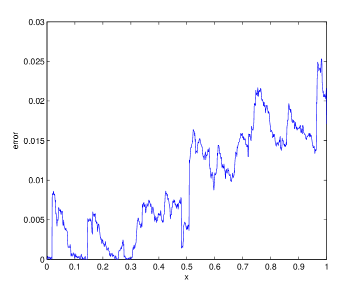
The numerical study is performed for the above model. In Fig. 1, we take x0=10,y0=10x_{0}=10,y_{0}=10, α=1.5\alpha=1.5, M=100,N=1000M=100,N=1000 with different ε\varepsilon, The macro and micro time steps are Δ​t=0.001\Delta t=0.001, δ​t=Δ​t/M\delta t=\Delta t/M, respectively. The results, presented in Fig. 1, indicate that the solution of slow component produced by the PIM approximates the solution of effective equation. It is worth emphasizing that even if the invariant measures cannot be obtained explicitly, we can still detect slow variables by PIM method. In Fig. 2, we compute the LpL^{p} error between XnX_{n} and X¯n\bar{X}_{n} with p=1.2p=1.2 for different ε\varepsilon, where LpL^{p} error =∑k=1l|Xnk−X¯nk|p/l=\sum_{k=1}^{l}|X_{n}^{k}-\bar{X}_{n}^{k}|^{p}/l. As seen in Fig. 2 , the LpL^{p} error is larger as the ε\varepsilon becomes larger.

Refer to caption
(a) ε=0.1\varepsilon=0.1
Refer to caption
(b) ε=0.01\varepsilon=0.01
Figure 1: Compare the effective dynamics with the stochastic projective integration schemes.
Refer to caption
(a) ε=0.1\varepsilon=0.1
Refer to caption
(b) ε=0.01\varepsilon=0.01
Figure 2: The LpL^{p} error between XnX_{n} and X¯n\bar{X}_{n} for ε=0.1\varepsilon=0.1.
Table 1: the error EpE_{p} for different ll.
   l       1       2       3       4       5   
   p=1.4       0.3324       0.1711       0.0759       0.0444       0.0270   
Refer to caption
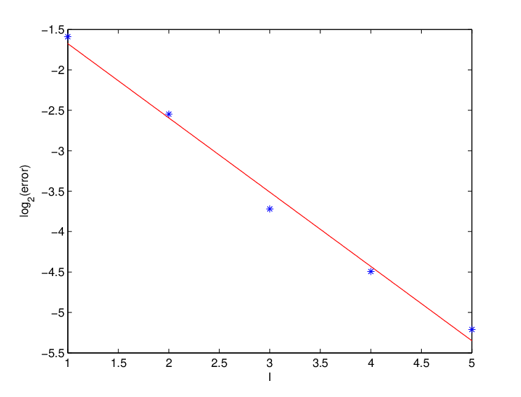
Figure 3: The logarithm error log2⁡(Ep)\log_{2}(E_{p}) with p=1.4p=1.4, ε=0.1\varepsilon=0.1 . The solid line is a line with s​l​o​p​e=0.92slope=0.92.

Suppose that T=1T=1 is fixed, we want to bound the error by 𝕆⁡(2−l)\mathbb{O}(2^{-l}) for l=1,2,…l=1,2,..., then the optimal choice is to take δ​t=𝒪⁡(2−lp​α2)\delta t=\mathcal{O}(2^{-\frac{l}{p}\alpha_{2}}) and M=𝒪⁡(2(2+α2)​lp)M=\mathcal{O}(2^{(2+\alpha_{2})\frac{l}{p}}) by simple analysis. Here we compute the following error estimate averaged with the K=1000K=1000 sample paths of the macro dynamics

Ep=1K​∑k=1K(∑n≤TΔΔT​|Xnk−X¯nk|p).E_{p}=\frac{1}{K}\sum_{k=1}^{K}\left(\sum_{n\leq\frac{T}{\Delta}}\frac{\Delta}{T}|X_{n}^{k}-\bar{X}_{n}^{k}|^{p}\right).

The errors EpE_{p} for different ll are listed in Table 1, and the logarithm errors log2⁡(Ep)\log_{2}(E_{p}) are also shown in Fig. 3. We observe that the errors are agree with our theoretical result 𝕆⁡(2−l)\mathbb{O}(2^{-l}) .

6 Discussion

In this paper, we studied the strong and weak convergences of projective integration methods for the multiscale stochastic dynamical systems driven by α\alpha-stable processes, which were used to estimate the effect that the fast components have on slow ones. Moreover, we obtained the ppth moment error bounds between the solution of slow component produced by the PIM and the solution of effective dynamical system with p∈(1,α)p\in\left(1,\alpha\right). Our scheme provided a new numerical method to obtain the slow component even if the invariant measure was unknown.

By reexamining the argument of the above results, the parameter value α\alpha of noise terms in slow component and fast component can be different, for example

{d​Xtε=f1(Xεt,Yεt)dt+σ1dLα1t,Xε0=x0∈ℝn,d​Ytε=1εf2(Xεt,Yεt)dt+σ2ε1αdLα2t,Yε0=y0∈ℝm,\left\{\begin{aligned} dX^{\varepsilon}_{t}&=f_{1}(X^{\varepsilon}_{t},Y^{\varepsilon}_{t})dt+\sigma_{1}dL^{\alpha_{1}}_{t},~~X^{\varepsilon}_{0}=x_{0}\in\mathbb{R}^{n},\\ dY^{\varepsilon}_{t}&=\frac{1}{\varepsilon}f_{2}(X^{\varepsilon}_{t},Y^{\varepsilon}_{t})dt+\frac{\sigma_{2}}{\varepsilon^{\frac{1}{\alpha}}}dL^{\alpha_{2}}_{t},~~Y^{\varepsilon}_{0}=y_{0}\in\mathbb{R}^{m},\end{aligned}\right. (6.1)

where Ltα1,Ltα2L^{\alpha_{1}}_{t},L^{\alpha_{2}}_{t} are independent nn and mm dimensional symmetric α\alpha-stable processes with triplets (0,0,ν1)(0,0,\nu_{1}) and (0,0,ν2)(0,0,\nu_{2}), respectively.

There are some limitations for this paper. The condition p∈(1,α)p\in(1,\alpha) plays an important role in deriving the effective dynamical system. Therefore, for the technical reason, it seems hard to show Lemma 1 and Lemma 12 with p∈(0,1)p\in(0,1). For such a case, it is necessary to find some new approaches to study. It is an open problem for the convergence in probability of averaging principle for the systems (6.2).

As an extension of the model, we also will study equations like (6.2) on the diffusive time scale, i.e.,

{d​Xtε=f1(Xεt,Yεt)dt++σ1dLtα1,Xε0=x0∈ℝn,d​Ytε=1ε2f2(Xεt,Yεt)dt+σ2ε2αdLα2t,Yε0=y0∈ℝm,\left\{\begin{aligned} dX^{\varepsilon}_{t}&=f_{1}(X^{\varepsilon}_{t},Y^{\varepsilon}_{t})dt++\sigma_{1}dL_{t}^{{\alpha}_{1}},~~X^{\varepsilon}_{0}=x_{0}\in\mathbb{R}^{n},\\ dY^{\varepsilon}_{t}&=\frac{1}{\varepsilon^{2}}f_{2}(X^{\varepsilon}_{t},Y^{\varepsilon}_{t})dt+\frac{\sigma_{2}}{\varepsilon^{\frac{2}{\alpha}}}dL^{\alpha_{2}}_{t},~~Y^{\varepsilon}_{0}=y_{0}\in\mathbb{R}^{m},\end{aligned}\right. (6.2)

Some new theoretical and numerical results will be reported in the forthcoming manuscript.

Acknowledgements. The research of Y. Zhang was supported by the NSFC grant 11901202. The research of X. Wang was supported by the NSFC grant 11901159. The research of J. Duan was supported by the NSF-DMS no. 1620449 and NSFC grant. 11531006 and 11771449.

Reference

References

  • [1] R. Bertram and J. E. Rubin, Multi-timescale systems and fast-slow analysis, Math. Biosci., 287(2017), pp. 105-121.
  • [2] E. A. Mastny, E. L. Haseltine and J. B. Rawlings, Two classes of quasi-steady-state model reductions for stochastic kinetics, J. Chem. Phys., 127(2007), pp. 094106.
  • [3] P. Ditlevsen, Observation of α\alpha-stable noise induced millennial climate changes from an ice record, Geophys. Res. Lett., 26(1999), pp. 1441-1444.
  • [4] E. Harvey, V. Kirk, M. Wechselberger and J. Sneyd, Multiple time scales, mixed mode oscillations and canards in models of intracellular calcium dynamics, J. Nonlinear Sci. 21(2011), pp. 639-683.
  • [5] R.Z. Khasminskii, On an averging principle for Itô stochastic differential equations, Kibernetica, 4(1968), pp. 260¨C279.
  • [6] Y. Kifer, Diffusion approximation for slow motion in fully coupled averaging, Proba. Theor. Relat. Fields, 129(2004), pp. 157¨C181.
  • [7] S. Cerrai, Averaging principle for systems of reaction-diffusion equations with polynomial nonlinearities perturbed by multiplicative noise, SIAM J. Math. Anal., 43(2011), pp. 2482-2518.
  • [8] S. Cerrai, M. Freidlin, Averaging principle for stochastic reaction-diffusion equations, Probab. Theory Related Fields, 144(2009), pp. 137-177.
  • [9] H. Fu, L. Wan, J. Liu, X. Liu, Weak order in averaging principle for stochastic wave equation with a fast oscillation, Stochastic Process. Appl., 128(2018), pp. 2557-2580.
  • [10] W. Wang and A.J. Roberts, Average and deviation for slow-fast stochastic partial differential equations, J. Differential Equations, 253(2012, pp. 1265-1286.
  • [11] G. A. Pavliotis and A. M. Stuart, Multiscale methods: averaging and homogenization, Springer, New York, 2008.
  • [12] D. Liu, Strong convergence rate of principle of averaging for jump-diffusion processes, Front. Math. China, 7(2012), pp. 305-320.
  • [13] J. Xu, Y. Miao and J. Liu, Strong averaging principle for two-time-scale non-autonomous stochastic FitzHugh-Nagumo system with jumps, J. Math. Phys., 57(2016), pp. 092704.
  • [14] D. Givon, Strong convergence rate for two-time-scale jump-diffusion stochastic differential systems, Multiscale Model. Simul., 6(2007), pp. 577-594.
  • [15] D. Applebaum, Lévy Processes and Stochastic Calculus, Cambridge University Press, 2009.
  • [16] J. Bao, G. Yin and C. Yuan, Two-time-scale stochastic partial differential equations driven by α\alpha-stable noises: Averaging principles, Bernoulli, 23(2018), pp. 645-669.
  • [17] Y. Zhang, Z. Cheng, X. Zhang, X. Chen, J. Duan and X. Li, Data assimilation and parameter estimation for a multiscale stochastic system with ¦Á-stable Lévy noise, J. Stat. Mech. Theory Exp., (11)2017, pp. 113401.
  • [18] Y. Zhang, J. Duan and X. Li, Effective filtering analysis for non-Gaussian dynamic systems, Appl. Math. Opt., 2019, https://doi.org/10.1007/s00245-018-9552-3.
  • [19] X. Sun and J. Zhai, Averaging principle for stochastic real Ginzburg-Landau equation driven by α\alpha-stable process, Commun. Pure Appl. Anal., 19(2020), pp. 1291-1319.
  • [20] X. Sun, L. Xie and Y. Xie, Strong and weak convergence rates for slow-fast stochastic differential equations driven by α\alpha-stable process, https://arxiv.org/abs/2004.02595.
  • [21] E. Vanden-Eijnden, Numerical techniques for multi-scale dynamical systems with stochastic effects, Commun. math. sci., 1(2003), pp. 385-391.
  • [22] W. E and B. Engquist, Analysis of multiscale methods for stochastic differential equations, Commun. Pur. Appl. Math., 58(2005), pp. 1544-1585.
  • [23] D. Givon, I. G. Keverkidis and R. Kupferman, Strong convergence of projective integration schemes for singularly perturbed stochastic differential systems, Comm. Math. Sci., 4(2006): 707-729.
  • [24] J. Duan, An Introduction to Stochastic Dynamics, Cambridge University Press, UK, 2015.
  • [25] Long. X and X. Zhang, Ergodicity of stochastic differential equations with jumps and singular coefficients, Ann. Inst. H. Poincar¨¦ Probab. Statist., 56(2020), pp. 175-229.
  • [26] S. Albeverio, B. Rüdiger and J. Wu, Invariant measures and symmetry property of Lévy type operators, Potential Anal., 13(2000), pp. 147-168.