跳到论文正文
W Papers独立论文阅读器 arXiv:2004.10499 论文正文 计算阅读时间 · 0%
引用这篇论文根据当前论文元数据生成,正式投稿前建议核对。


License: arXiv.org perpetual non-exclusive license
arXiv:2004.10499v1 [cs.IT] 22 Apr 2020

Hardware and Interference Limited Cooperative CR-NOMA Networks under Imperfect SIC and CSI

Sultangali Arzykulov    Galymzhan Nauryzbayev    Affiliation: Abdulkadir Celik, and Ahmed M. Eltawil,
Abstract

The conflation of cognitive radio (CR) and non-orthogonal multiple access (NOMA) concepts is a promising approach to fulfill the massive connectivity goals of future networks given the spectrum scarcity. Accordingly, this letter investigates the outage performance of imperfect cooperative CR-NOMA networks under hardware impairments and interference. Our analysis is involved with the derivation of the end-to-end outage probability (OP) for secondary NOMA users by accounting for imperfect channel state information (CSI), as well as the residual interference caused by successive interference cancellation (SIC) errors and coexisting primary/secondary users. The numerical results validated by Monte Carlo simulations show that CR-NOMA network provides a superior outage performance over orthogonal multiple access. As imperfections become more significant, CR-NOMA is observed to deliver relatively poor outage performance.

Index Terms:
Cognitive radio, cooperative non-orthogonal multiple access, outage probability, hardware impairment.

I Introduction

The ambitious quality-of-service (QoS) demands of future wireless networks poses daunting challenges, especially under the ever-increasing number of devices connected to the Internet [1]. This consequently leads to two problems: spectrum scarcity and interference-limited networks. Spectrum scarcity has been mostly studied in the realm of cognitive radio (CR) networks where unlicensed/secondary users are permitted to operate on spectrum bands licensed to primary users in an opportunistic and non-intrusive manner [2]. Alternatively, non-orthogonal multiple access (NOMA) schemes have also recently received attention as a promising technique to mitigate the inability of orthogonal multiple access (OMA) schemes to support massive connectivity [3]. On the transmitter side, the NOMA scheme superposes messages of intended users with distinctive power allocation (PA) weights based on their channel quality. On the receiver side, the intended signal is extracted by decoding the transmitted broadcast message using successive interference cancellation (SIC).

Therefore, the conflation of CR and NOMA concepts (CR-NOMA) is regarded as a potential solution to the problems mentioned above. Existing literature on cooperative CR-NOMA networks mostly deals with simple scenarios under ideal cases without paying sufficient attention to practical limitations in terms of channel and hardware impairments [4, 5, 6, 7]. Accordingly, this letter investigates the outage performance of a generic and imperfect CR-NOMA, where non-ideality is modeled by accounting for hardware impairments (HIs), channel state information (CSI) imperfections, and residual interference due to the SIC error propagation. Ensuring that primary traffic is protected, our analysis also tackles the random interference caused by coexisting primary/secondary users. The numerical results validated by Monte Carlo simulations show that the CR-NOMA network provides a superior outage performance over orthogonal multiple access, which degrades with CSI and SIC imperfections.

II System Model
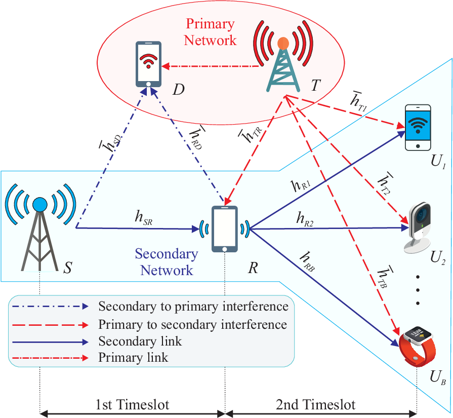
Refer to caption
Figure 1: The proposed underlay CR-NOMA network.

II-A Channel Model

We consider a downlink CR-NOMA network that consists of primary and secondary networks as illustrated in Fig. 1. The primary network comprises of primary transmitter (TT) and destination (DD) nodes. On the other hand, the secondary network consists of a source (SS), a relay (RR) that cooperates with SS in a half-duplex decode-and-forward (DF) mode, and BB secondary NOMA users. The cooperation occurs in two time slots; The broadcast signal transmitted by SS in the first time slot is re-transmitted to BB NOMA users in the second time slot. Channel gains among the nodes are modeled as h¯i∼𝒞​𝒩​(0,1),∀i∈{S​D,S​R,R​D,R​1,…,R​B,T​R,T​1,…,T​B}\bar{h}_{i}\sim\mathcal{CN}(0,1),\penalty\ \forall i\in\{SD,SR,RD,R1,\ldots,RB,TR,T1,\ldots,TB\}. Moreover, the distance between the corresponding nodes and the path-loss exponent are denoted by did_{i} and τ\tau, respectively. To capture CSI imperfections, we model channel coefficients using the minimum mean square error (MMSE) channel estimator as h¯i=hi+ei\bar{h}_{i}=h_{i}+e_{i}, where hi∼𝒞​𝒩​(0,σhi2)h_{i}\sim\mathcal{CN}(0,\sigma_{h_{i}}^{2}) and ei∼𝒞​𝒩​(0,ζi)e_{i}\sim\mathcal{CN}(0,\zeta_{i}) are the estimated channel coefficient and channel estimation error with variance σhi2\sigma_{h_{i}}^{2} and ζi\zeta_{i}, respectively. The error variance is modeled as ζi≜θ​ρ−κ\zeta_{i}\triangleq\theta\rho^{-\kappa} where ρ=Pσ2\rho=\frac{P}{\sigma^{2}} is the transmitted signal-to-noise ratio (SNR), and κ⩾0\kappa\geqslant 0, θ>0\theta>0 [8]. Indeed, this model describes various CSI acquisition scenarios: a) ζ\zeta is a function of ρ\rho for κ≠0\kappa\neq 0, and b) ζ\zeta is independent of ρ\rho for κ=0\kappa=0. Following from the underlay CR paradigm, it is also assumed that the transmit power of a secondary node j∈{R,S}j\in\{R,S\} is restricted as [9] Pj⩽min⁡(P¯j,IITC,j|h¯j​D|2)P_{j}\leqslant\min\left(\bar{P}_{j},\frac{I_{\text{ITC},j}}{|\bar{h}_{jD}|^{2}}\right), where P¯j\bar{P}_{j} stands for the maximum transmit power at node jj and IITC,jI_{\text{ITC},j} denotes the interference temperature constraint (ITC) at DD caused by node jj.

II-B Transmission Protocol

In the first time slot of the proposed CR-NOMA relaying model, SS broadcasts ∑b=1Bαb​xb\sum_{b=1}^{B}\sqrt{\alpha_{b}}x_{b} to RR, where αb\alpha_{b} is the PA factor11 1 Similar to [10], we allocate the power based on the QoS requirements imposed at secondary NOMA users. of UbU_{b} such that α1>…>αb>…>αB\alpha_{1}>\ldots>\alpha_{b}>\ldots>\alpha_{B} and ∑b=1Bαb=1\sum_{b=1}^{B}\alpha_{b}=1, and xbx_{b} is the message dedicated to UbU_{b} with 𝔼⁡(|xb|2)=1\mathbb{E}(|x_{b}|^{2})=1.

Considering CSI imperfections and aggregate distortion noise, the received signal at RR can be written as

yR=\displaystyle y_{R}= (hS​R+eS​R)​P~S​(∑b=1Bαb​xb+ηS​R)\displaystyle\left(h_{SR}+e_{SR}\right)\sqrt{\tilde{P}_{S}}\left(\sum_{b=1}^{B}\sqrt{\alpha_{b}}x_{b}+\eta_{SR}\right)
+h¯T​R​P~T​(xT+ηT)+nR,\displaystyle+\bar{h}_{TR}\sqrt{\tilde{P}_{T}}\left(x_{T}+\eta_{T}\right)+n_{R}, (1)

where P~i=Pidi​Rτ\tilde{P}_{i}=\frac{P_{i}}{d_{iR}^{\tau}}, i∈{S,T}i\in\{S,T\}; η(⋅)∼𝒞​𝒩​(0,ϕ(⋅)2)\eta_{(\cdot)}\sim\mathcal{CN}\left(0,\phi^{2}_{(\cdot)}\right) denotes the aggregate distortion noise from transceiver; ϕ(⋅)\phi_{(\cdot)} = ϕt2+ϕr2\sqrt{\phi^{2}_{t}+\phi^{2}_{r}} is the aggregate HI level from the transmitter and receiver [11]; n(⋅)∼𝒞​𝒩​(0,σ(⋅)2)n_{(\cdot)}\sim\mathcal{CN}(0,\sigma_{(\cdot)}^{2}) denotes the additive white Gaussian noise (AWGN) term at each receiver node; PTP_{T} and xTx_{T} stand for the transmit power at TT and the message dedicated to DD, respectively. Then, the instantaneous signal-to-interference-distortion-noise-ratio (SIDNR) to decode xjx_{j}, 1≤j≤b<B1\leq j\leq b<B, at RR can be expressed by

γR,j\displaystyle\gamma_{R,j} =αj​PS​|hS​R|2𝒜​PS​|hS​R|2+𝒞​PS+𝒟R​P~T​|h¯T​R|2+dS​Rτ​σR2,\displaystyle=\frac{\alpha_{j}P_{S}\left|h_{SR}\right|^{2}}{\mathcal{A}P_{S}\left|h_{SR}\right|^{2}+\mathcal{C}P_{S}+\mathcal{D}_{R}\tilde{P}_{T}\left|\bar{h}_{TR}\right|^{2}+d^{\tau}_{SR}\sigma^{2}_{R}}, (2)

where 𝒜=Ωj+Ω~j+ϕS​R2\mathcal{A}=\Omega_{j}+\tilde{\Omega}_{j}+\phi^{2}_{SR}; Ωj=∑n=j+1Bαn\Omega_{j}=\sum_{n=j+1}^{B}\alpha_{n}; Ω~j=∑n~=1j−1϶n~αn~\tilde{\Omega}_{j}=\sum_{\tilde{n}=1}^{j-1}\backepsilon_{\tilde{n}}\alpha_{\tilde{n}}, 0<϶n~<10<\backepsilon_{\tilde{n}}<1, where ϶n~=0\backepsilon_{\tilde{n}}=0 and ϶n~=1\backepsilon_{\tilde{n}}=1 indicate the perfection and absence of SIC, respectively; 𝒞=ζS​R+ζS​R​ϕS​R2\mathcal{C}=\zeta_{SR}+\zeta_{SR}\phi^{2}_{SR} and 𝒟R=dS​Rτ​dT​R−τ​(1+ϕT​R2)\mathcal{D}_{R}=d^{\tau}_{SR}d^{-\tau}_{TR}\left(1+\phi^{2}_{TR}\right). Furthermore, by assuming imperfect detection of xjx_{j}, RR decodes the message of user BB with the SIDNR of

γR,B\displaystyle\hskip-5.69046pt\gamma_{R,B} =αB​PS​|hS​R|2𝒜~​PS​|hS​R|2+𝒞​PS+𝒟R​P~T​|h¯T​R|2+dS​Rτ​σR2,\displaystyle=\frac{\alpha_{B}P_{S}\left|h_{SR}\right|^{2}}{\mathcal{\tilde{A}}P_{S}\left|h_{SR}\right|^{2}+\mathcal{C}P_{S}+\mathcal{D}_{R}\tilde{P}_{T}\left|\bar{h}_{TR}\right|^{2}+d^{\tau}_{SR}\sigma^{2}_{R}}, (3)

where 𝒜~=(Ω~B+ϕS​R2)\mathcal{\tilde{A}}=\left(\tilde{\Omega}_{B}+\phi^{2}_{SR}\right) and Ω~B=∑n~=1B−1϶n~αn~\tilde{\Omega}_{B}=\sum_{\tilde{n}=1}^{B-1}\backepsilon_{\tilde{n}}\alpha_{\tilde{n}}.

In the second time slot, RR relays the decoded signal ∑b=1Bβb​x~b\sum_{b=1}^{B}\sqrt{\beta_{b}}\tilde{x}_{b} to BB NOMA users, where βb\beta_{b}, with ∑b=1Bβb=1\sum_{b=1}^{B}\beta_{b}=1, is the PA factor of UbU_{b}. Hence, the received signal at UbU_{b} can be written as

yb\displaystyle y_{b} =(hR​b+eb)​P~R​(∑j=1Bβj​xj+ηb)\displaystyle=\left(h_{Rb}+e_{b}\right)\sqrt{\tilde{P}_{R}}\left(\sum_{j=1}^{B}\sqrt{\beta_{j}}x_{j}+\eta_{b}\right)
+h¯T​b​P~T​(xT+ηT)+nb,\displaystyle\penalty\ \penalty\ \penalty\ +\bar{h}_{Tb}\sqrt{\tilde{P}_{T}}\left(x_{T}+\eta_{T}\right)+n_{b}, (4)

where P~i=Pidi​bτ\tilde{P}_{i}=\frac{P_{i}}{d^{\tau}_{ib}}, i∈{R,T}i\in\{R,T\}. Then, we can write the SIDNR for UbU_{b} to detect the message of UjU_{j} as follows

γb,j\displaystyle\gamma_{b,j} =βj​PR​|hR​b|2𝒥b​PR​|hR​b|2+𝒢b​PR+𝒟b​P~T​|h¯T​b|2+dR​bτ​σb2,\displaystyle=\frac{\beta_{j}P_{R}\left|h_{Rb}\right|^{2}}{\mathcal{J}_{b}P_{R}\left|h_{Rb}\right|^{2}+\mathcal{G}_{b}P_{R}+\mathcal{D}_{b}\tilde{P}_{T}\left|\bar{h}_{Tb}\right|^{2}+d^{\tau}_{Rb}\sigma^{2}_{b}}, (5)

where β1>βj>βb>βB\beta_{1}>\beta_{j}>\beta_{b}>\beta_{B}; ∀b∈{1,…,B}\forall b\in\{1,\ldots,B\}; 𝒥b=(Ωj+Ω~j+ϕb2)\mathcal{J}_{b}=\left(\Omega_{j}+\tilde{\Omega}_{j}+\phi^{2}_{b}\right); Ωj=∑n=j+1bβn\Omega_{j}=\sum_{n=j+1}^{b}\beta_{n}; Ω~j=∑n~=1j−1϶n~βn~\tilde{\Omega}_{j}=\sum_{\tilde{n}=1}^{j-1}\backepsilon_{\tilde{n}}\beta_{\tilde{n}}; 𝒢b=(ζb+ζb​ϕb2)\mathcal{G}_{b}=\left(\zeta_{b}+\zeta_{b}\phi^{2}_{b}\right) and 𝒟b=dR​bτ​dT​b−τ​(1+ϕT​b2)\mathcal{D}_{b}=d^{\tau}_{Rb}d^{-\tau}_{Tb}\left(1+\phi^{2}_{Tb}\right). Finally, after decoding messages of B−1B-1 NOMA users, UBU_{B} detects its own message with

γB\displaystyle\hskip-5.69046pt\gamma_{B} =βB​PR​|hR​B|2𝒥B​PR​|hR​B|2+𝒢B​PR+𝒟B​P~T​|h¯T​B|2+dR​Bτ​σB2,\displaystyle=\frac{\beta_{B}P_{R}\left|h_{RB}\right|^{2}}{\mathcal{J}_{B}P_{R}\left|h_{RB}\right|^{2}+\mathcal{G}_{B}P_{R}+\mathcal{D}_{B}\tilde{P}_{T}\left|\bar{h}_{TB}\right|^{2}+d^{\tau}_{RB}\sigma^{2}_{B}}, (6)

where 𝒥B=Ω~B+ϕB2\mathcal{J}_{B}=\tilde{\Omega}_{B}+\phi^{2}_{B}; Ω~B=∑n~=1B−1϶n~βn~\tilde{\Omega}_{B}=\sum_{\tilde{n}=1}^{B-1}\backepsilon_{\tilde{n}}\beta_{\tilde{n}}. Considering the dual-hop communication, the achievable rate at UjU_{j} is calculated as

ℛj=12​log2​[1+min⁡(γR,j,γb,j)], 1≤j≤b≤B.\displaystyle\mathcal{R}_{j}=\frac{1}{2}\log_{2}\left[1+\min\left(\gamma_{R,j},\gamma_{b,j}\right)\right],\penalty\ 1\leq j\leq b\leq B. (7)

III Outage Analysis

The outage at UjU_{j} occurs when the achievable rate at UjU_{j} is below a predefined rate threshold ℛth,j\mathcal{R}_{{\text{th}},j}. Following from (7), the OP of UjU_{j} can be written as

Pout,j\displaystyle P_{{\text{out}},j} =Pr[12log2[1+min(γR,j,γb,j)]<ℛth,j]\displaystyle={\text{Pr}}\left[\frac{1}{2}\log_{2}\left[1+\min\left(\gamma_{R,j},\gamma_{b,j}\right)\right]<\mathcal{R}_{{\text{th}},j}\right]
=1−Pr[min(γR,j,γb,j)>ψj]\displaystyle=1-{\text{Pr}}\left[\min\left(\gamma_{R,j},\gamma_{b,j}\right)>\psi_{j}\right]
=FγR,j​(ψj)+Fγj​(ψj)−FγR,j​(ψj)​Fγj​(ψj),\displaystyle=F_{\gamma_{R,j}}(\psi_{j})+F_{\gamma_{j}}(\psi_{j})-F_{\gamma_{R,j}}(\psi_{j})F_{\gamma_{j}}(\psi_{j}), (8)

where ψj=22​ℛth,j−1\psi_{j}=2^{2\mathcal{R}_{{\text{th}},j}}-1 denotes the predefined SNR threshold at UjU_{j}. Now, considering the ITC imposed at DD, we can write the CDF of the RV γR,j\gamma_{R,j} as in (III), where X=|hS​R|2X=\left|h_{SR}\right|^{2}, Y=|h¯S​D|2Y=\left|\bar{h}_{SD}\right|^{2} and Z=|h¯P​R|2Z=\left|\bar{h}_{PR}\right|^{2} follow the exponential distribution with parameter λ\lambda; 𝒦c=𝒟R​P~T​ψjd⁡(αj−𝒜​ψj)\mathcal{K}_{c}=\frac{\mathcal{D}_{R}\tilde{P}_{T}\psi_{j}}{d\left(\alpha_{j}-\mathcal{A}\psi_{j}\right)}; ℳc=ψj​dS​Rτ​σj2d⁡(αj−𝒜​ψj)\mathcal{M}_{c}=\frac{\psi_{j}d^{\tau}_{SR}\sigma^{2}_{j}}{d\left(\alpha_{j}-\mathcal{A}\psi_{j}\right)}, with c=dc=d, c∈{Δ,Υ}c\in\{\Delta,\Upsilon\} and d∈{P¯S,IITC​dS​Dτ}d\in\{\bar{P}_{S},I_{\text{ITC}}d^{\tau}_{SD}\}; ℒ=𝒞​ψjαj−𝒜​ψj\mathcal{L}=\frac{\mathcal{C}\psi_{j}}{\alpha_{j}-\mathcal{A}\psi_{j}} and ΛS=IITC​dS​DτP¯S\Lambda_{S}=\frac{I_{\text{ITC}}d^{\tau}_{SD}}{\bar{P}_{S}}.

FγR,j​(ψj)\displaystyle F_{\gamma_{R,j}}(\psi_{j}) =Pr​[αj​P¯S​|hS​R|2𝒜​P¯S​|hS​R|2+𝒞​P¯S+𝒟R​P~T​|h¯T​R|2+dS​Rτ​σR2<ψj,P¯S<IITC​dS​Dτ|h¯S​D|2]\displaystyle={\text{Pr}}\left[\frac{\alpha_{j}\bar{P}_{S}\left|h_{SR}\right|^{2}}{\mathcal{A}\bar{P}_{S}\left|h_{SR}\right|^{2}+\mathcal{C}\bar{P}_{S}+\mathcal{D}_{R}\tilde{P}_{T}\left|\bar{h}_{TR}\right|^{2}+d^{\tau}_{SR}\sigma^{2}_{R}}<\psi_{j},\penalty\ \bar{P}_{S}<\frac{I_{\text{ITC}}d^{\tau}_{SD}}{|\bar{h}_{SD}|^{2}}\right]
+Pr​[αj​IITC​dS​Dτ​|hS​R|2|h¯​S​D|2𝒜​IITC​dS​Dτ​|hS​R|2|h¯​S​D|2+𝒞​IITC​dS​Dτ|h¯​S​D|2+𝒟R​P~T​|h¯T​R|2+dS​Rτ​σR2​<ψj,P¯S>​IITC​dS​Dτ|h¯S​D|2]\displaystyle\penalty\ \penalty\ \penalty\ +{\text{Pr}}\left[\frac{\frac{\alpha_{j}I_{\text{ITC}}d^{\tau}_{SD}\left|h_{SR}\right|^{2}}{|\bar{h}{SD}|^{2}}}{\frac{\mathcal{A}I_{\text{ITC}}d^{\tau}_{SD}\left|h_{SR}\right|^{2}}{|\bar{h}{SD}|^{2}}+\frac{\mathcal{C}I_{\text{ITC}}d^{\tau}_{SD}}{|\bar{h}{SD}|^{2}}+\mathcal{D}_{R}\tilde{P}_{T}\left|\bar{h}_{TR}\right|^{2}+d^{\tau}_{SR}\sigma^{2}_{R}}<\psi_{j},\penalty\ \bar{P}_{S}>\frac{I_{\text{ITC}}d^{\tau}_{SD}}{|\bar{h}_{SD}|^{2}}\right]
=Pr​[X<Z​𝒦Δ+ℳΔ+ℒ,Y<ΛS]⏟Δ+Pr​[X<Z​Y​𝒦Υ+Y​ℳΥ+ℒ,Y>ΛS]⏟Υ,\displaystyle=\underbrace{{\text{Pr}}\left[X<Z\mathcal{K}_{\Delta}+\mathcal{M}_{\Delta}+\mathcal{L},Y<\Lambda_{S}\right]}_{\text{$\Delta$}}+\underbrace{{\text{Pr}}\left[X<ZY\mathcal{K}_{\Upsilon}+Y\mathcal{M}_{\Upsilon}+\mathcal{L},Y>\Lambda_{S}\right]}_{\text{$\Upsilon$}}, (9)


Proposition 1

The CDF of γR,j\gamma_{R,j} can be derived in its closed-form as

FγR,j\displaystyle F_{\gamma_{R,j}} (ψj)=1−λz​e−λx​(ℳΔ+ℒ)λz+λx​𝒦Δ​(1−e−λy​ΛS)\displaystyle(\psi_{j})=1-\frac{\lambda_{z}e^{-\lambda_{x}\left(\mathcal{M}_{\Delta}+\mathcal{L}\right)}}{\lambda_{z}+\lambda_{x}\mathcal{K}_{\Delta}}\left(1-e^{-\lambda_{y}\Lambda_{S}}\right)
+λy​λz​Ei​[−μS​ξS]λx​𝒦Υ​e−ΛS​(λy+λx​ℳΥ)−λx​ℒ+μS​ξS.\displaystyle+\frac{\lambda_{y}\lambda_{z}\text{Ei}\left[-\mu_{S}\xi_{S}\right]}{\lambda_{x}\mathcal{K}_{\Upsilon}}e^{-\Lambda_{S}\left(\lambda_{y}+\lambda_{x}\mathcal{M}_{\Upsilon}\right)-\lambda_{x}\mathcal{L}+\mu_{S}\xi_{S}}. (10)

Proof:

See Appendix A. ∎

Following from (5), the CDF of γb,j\gamma_{b,j} can be described as

Fγb,j​(ψj)\displaystyle F_{\gamma_{b,j}}(\psi_{j}) =Pr​[Q<W​𝒮Θ+𝒪Θ+𝒯,V<ΛR]⏟Θ\displaystyle=\underbrace{{\text{Pr}}\left[Q<W\mathcal{S}_{\Theta}+\mathcal{O}_{\Theta}+\mathcal{T},V<\Lambda_{R}\right]}_{\text{$\Theta$}}
+Pr​[Q<W​V​𝒮Φ+V​𝒪Φ+𝒯,V>ΛR]⏟Φ,\displaystyle+\underbrace{{\text{Pr}}\left[Q<WV\mathcal{S}_{\Phi}+V\mathcal{O}_{\Phi}+\mathcal{T},V>\Lambda_{R}\right]}_{\text{$\Phi$}}, (11)

where Q=|hR​b|2Q=|h_{Rb}|^{2}; V=|h¯R​D|2V=|\bar{h}_{RD}|^{2}; W=|h¯T​b|2W=|\bar{h}_{Tb}|^{2}; 𝒮k=𝒟b​P~T​ψjl⁡(βb−𝒥b​ψj)\mathcal{S}_{k}=\frac{\mathcal{D}_{b}\tilde{P}_{T}\psi_{j}}{l\left(\beta_{b}-\mathcal{J}_{b}\psi_{j}\right)}; 𝒪k=dR​bτ​σb2​ψjl⁡(βb−𝒥b​ψj)\mathcal{O}_{k}=\frac{d^{\tau}_{Rb}\sigma^{2}_{b}\psi_{j}}{l\left(\beta_{b}-\mathcal{J}_{b}\psi_{j}\right)}, with k=lk=l, k∈{Θ,Φ}k\in\{\Theta,\Phi\} and l∈{P¯R,IITC​dR​Dτ}l\in\{\bar{P}_{R},I_{\text{ITC}}d^{\tau}_{RD}\}; 𝒯=𝒢b​ψjβb−𝒥b​ψj\mathcal{T}=\frac{\mathcal{G}_{b}\psi_{j}}{\beta_{b}-\mathcal{J}_{b}\psi_{j}} and ΛR=IITC​dR​DτP¯R\Lambda_{R}=\frac{I_{\text{ITC}}d^{\tau}_{RD}}{\bar{P}_{R}}.

Proposition 2

The closed-from expression for the CDF of γb,j\gamma_{b,j} can be written as

Fγb,j\displaystyle F_{\gamma_{b,j}} (ψj)=1−λw​e−λq​(𝒪Θ+𝒯)λw+λq​𝒮Θ​(1−e−λv​ΛR)\displaystyle(\psi_{j})=1-\frac{\lambda_{w}e^{-\lambda_{q}\left(\mathcal{O}_{\Theta}+\mathcal{T}\right)}}{\lambda_{w}+\lambda_{q}\mathcal{S}_{\Theta}}\left(1-e^{-\lambda_{v}\Lambda_{R}}\right)
+λv​λw​Ei​[−μR​ξR]λq​𝒮Φ​e−ΛR​(λv+λq​𝒪Φ)−λq​𝒯+μR​ξR.\displaystyle+\frac{\lambda_{v}\lambda_{w}\text{Ei}\left[-\mu_{R}\xi_{R}\right]}{\lambda_{q}\mathcal{S}_{\Phi}}e^{-\Lambda_{R}\left(\lambda_{v}+\lambda_{q}\mathcal{O}_{\Phi}\right)-\lambda_{q}\mathcal{T}+\mu_{R}\xi_{R}}. (12)
Proof:

See Appendix B. ∎

Lastly, the exact OP of UjU_{j} can be derived after substituting (1) and (2) into (III). Similarly, the OP of the UMU_{M} can be derived by using (2) and (6) and following the same procedure in obtaining the OP of UjU_{j}. Then, following the similar approach as in Appendix A, the CDFs of the RV γR,B\gamma_{R,B} can be derived in closed-form as

FγR,B\displaystyle F_{\gamma_{R,B}} (ψB)=1−λz​e−λx​(ℋΨ+ℐ)λz+λx​ℰΨ​(1−e−λy​ΛS)\displaystyle(\psi_{B})=1-\frac{\lambda_{z}e^{-\lambda_{x}\left(\mathcal{H}_{\Psi}+\mathcal{I}\right)}}{\lambda_{z}+\lambda_{x}\mathcal{E}_{\Psi}}\left(1-e^{-\lambda_{y}\Lambda_{S}}\right)
+λy​λz​Ei​[−μ¯S​ξ¯S]λx​ℰΠ​e−ΛS​(λy+λx​ℋΠ)−λx​ℐ+μ¯S​ξ¯S,\displaystyle+\frac{\lambda_{y}\lambda_{z}\text{Ei}\left[-\bar{\mu}_{S}\bar{\xi}_{S}\right]}{\lambda_{x}\mathcal{E}_{\Pi}}e^{-\Lambda_{S}\left(\lambda_{y}+\lambda_{x}\mathcal{H}_{\Pi}\right)-\lambda_{x}\mathcal{I}+\bar{\mu}_{S}\bar{\xi}_{S}}, (13)

where ℰm=𝒟R​P~T​ψBd⁡(αB−𝒜~​ψB)\mathcal{E}_{m}=\frac{\mathcal{D}_{R}\tilde{P}_{T}\psi_{B}}{d\left(\alpha_{B}-\mathcal{\tilde{A}}\psi_{B}\right)}; ℋm=dS​Rτ​σB2​ψBd⁡(αB−𝒜~​ψB)\mathcal{H}_{m}=\frac{d^{\tau}_{SR}\sigma^{2}_{B}\psi_{B}}{d\left(\alpha_{B}-\mathcal{\tilde{A}}\psi_{B}\right)}, with m=dm=d, m∈{Ψ,Π}m\in\{\Psi,\Pi\} and d∈{P¯S,IITC​dS​Dτ}d\in\{\bar{P}_{S},I_{\text{ITC}}d^{\tau}_{SD}\}; ℐ=𝒞​ψℬαB−𝒜~​ψj\mathcal{I}=\frac{\mathcal{C\psi_{B}}}{\alpha_{B}-\mathcal{\tilde{A}}\psi_{j}}; μ¯S=λz+λx​ΛS​ℰΠ\bar{\mu}_{S}=\lambda_{z}+\lambda_{x}\Lambda_{S}\mathcal{E}_{\Pi}; ξ¯S=ℋΠℰΠ+λyλx​ℰΠ\bar{\xi}_{S}=\frac{\mathcal{H}_{\Pi}}{\mathcal{E}_{\Pi}}+\frac{\lambda_{y}}{\lambda_{x}\mathcal{E}_{\Pi}}. Moreover, ψB<αB𝒜~\psi_{B}<\frac{\alpha_{B}}{\mathcal{\tilde{A}}}, otherwise, FγR,B​(ψB)∼1F_{\gamma_{R,B}}(\psi_{B})\sim 1. Similarly, the CDF of γB\gamma_{B} is derived as

FγB\displaystyle F_{\gamma_{B}} (ψB)=1−λw¯​e−λq​(𝒪¯Ξ+𝒯¯)λw¯+λq¯​𝒮¯Ξ​(1−e−λv¯​ΛR)\displaystyle(\psi_{B})=1-\frac{\lambda_{\bar{w}}e^{-\lambda_{q}\left(\mathcal{\bar{O}}_{\Xi}+\mathcal{\bar{T}}\right)}}{\lambda_{\bar{w}}+\lambda_{\bar{q}}\mathcal{\bar{S}}_{\Xi}}\left(1-e^{-\lambda_{\bar{v}}\Lambda_{R}}\right)
+λv¯​λw¯​Ei​[−μR​ξR]λq¯​𝒮¯ℵ​e−ΛR​(λv¯+λq¯​𝒪¯ℵ)−λq¯​𝒯¯+μ¯R​ξ¯R,\displaystyle+\frac{\lambda_{\bar{v}}\lambda_{\bar{w}}\text{Ei}\left[-\mu_{R}\xi_{R}\right]}{\lambda_{\bar{q}}\mathcal{\bar{S}}_{\aleph}}e^{-\Lambda_{R}\left(\lambda_{\bar{v}}+\lambda_{\bar{q}}\mathcal{\bar{O}}_{\aleph}\right)-\lambda_{\bar{q}}\mathcal{\bar{T}}+\bar{\mu}_{R}\bar{\xi}_{R}}, (14)

where Q¯=|hR​B|2\bar{Q}=|h_{RB}|^{2}; W¯=|h¯T​B|2\bar{W}=|\bar{h}_{TB}|^{2}; 𝒮¯r=𝒟¯B​P~T​ψBn⁡(βB−𝒥¯B​ψB)\bar{\mathcal{S}}_{r}=\frac{\mathcal{\bar{D}}_{B}\tilde{P}_{T}\psi_{B}}{n\left(\beta_{B}-\mathcal{\bar{J}}_{B}\psi_{B}\right)}; 𝒪¯r=dR​Bτ​σB2​ψBn⁡(βB−𝒥¯B​ψB)\mathcal{\bar{O}}_{r}=\frac{d^{\tau}_{RB}\sigma^{2}_{B}\psi_{B}}{n\left(\beta_{B}-\mathcal{\bar{J}}_{B}\psi_{B}\right)}, with r=nr=n, r∈{Ξ,ℵ}r\in\{\Xi,\aleph\} and n∈{P¯R,IITC​dR​Dτ}n\in\{\bar{P}_{R},I_{\text{ITC}}d^{\tau}_{RD}\}; 𝒯¯=𝒢¯B​ψBβB−𝒥¯B​ψB\mathcal{\bar{T}}=\frac{\mathcal{\bar{G}}_{B}\psi_{B}}{\beta_{B}-\mathcal{\bar{J}}_{B}\psi_{B}}; μ¯R=λw¯+λq¯​ΛR​𝒮¯ℵ\bar{\mu}_{R}=\lambda_{\bar{w}}+\lambda_{\bar{q}}\Lambda_{R}\mathcal{\bar{S}}_{\aleph} and ξ¯R=𝒪¯ℵ𝒮¯ℵ+λv¯λq¯​𝒮¯ℵ\bar{\xi}_{R}=\frac{\mathcal{\bar{O}}_{\aleph}}{\mathcal{\bar{S}}_{\aleph}}+\frac{\lambda_{\bar{v}}}{\lambda_{\bar{q}}\mathcal{\bar{S}}_{\aleph}}. Notice that ψB<βB𝒥¯B\psi_{B}<\frac{\beta_{B}}{\mathcal{\bar{J}}_{B}}, otherwise, FγB​(ψB)∼1F_{\gamma_{B}}(\psi_{B})\sim 1. Finally, the exact OP of UBU_{B} can be derived by using (III) and (III).

Refer to caption
Figure 2: The OP versus the transmit SNR for NOMA and OMA users with IITC=20I_{\text{ITC}}=20 dB, ϕ=0\phi=0, ϶=0\backepsilon=0 and ζ=0\zeta=0.

IV Numerical Results

This section discusses the numerical results and validates that all theoretical analyses precisely match with Monte-Carlo simulations. We assume two secondary NOMA users22 2 In practice, it may not be feasible to consider many NOMA users due to the complexity and latency of SIC receivers, which increases non-linearly with the increase in the number of users [3]. In this work, SIC complexity especially becomes more significant because of the SIC error propagation., i.e., U1U_{1} and U2U_{2} with the following system settings; the same transmit power levels at SS and RR, i.e., P=PS=PRP=P_{S}=P_{R}; α1=β1=0.8\alpha_{1}=\beta_{1}=0.8; α2=β2=0.2\alpha_{2}=\beta_{2}=0.2; ℛ1=1\mathcal{R}_{1}=1 bps; ℛ2=1.5\mathcal{R}_{2}=1.5 bps; dS​R=dR​1=dR​2=dd_{SR}=d_{R1}=d_{R2}=d; dS​D=dR​D=dT​R=dT​1=dT​2=3​dd_{SD}=d_{RD}=d_{TR}=d_{T1}=d_{T2}=3d, where dd is assumed to be unity; τ=3\tau=3.

Fig. 2 compares the OP of users operating on OMA and NOMA. For the sake of a fair comparison, the QoS demands of cooperative OMA is set as two-fold of that used for cooperative NOMA. To demonstrate the ITC impacts on the OP of SUs, we consider the asymptotic case, where DD does not impose ITC, i.e., IITC=∞I_{\text{ITC}}=\infty. Fig. 2 shows that U1U_{1} achieves a lower OP than U2U_{2} since U1U_{1} is assigned with a lower rate and a higher PA factor. Also, notice that both NOMA users achieve a significantly lower OP than corresponding OMA modes. Additionally, we can observe that the ITC imposed at DD, i.e., IITCI_{\text{ITC}}, results in the saturation of OP curves. This implies that secondary transmitters cannot increase their transmission power above the ITC level in order not to cause harmful interference to DD. A noteworthy observation is that an increase in primary interference level results in the outage performance deterioration of SUs. For example, at transmit SNR of 2020 dB, U1U_{1} obtains the OP of 0.090.09, 0.120.12 and 0.620.62 without primary interference, PT=10P_{T}=10 dB and PT=25P_{T}=25 dB, respectively.

Refer to caption
Figure 3: The OP versus the transmit SNR for NOMA users with PT=10P_{T}=10 dB, IITC=∞I_{\text{ITC}}=\infty and ζ=0\zeta=0.

Fig. 3 presents the impact of hardware and SIC imperfections on the OP of NOMA users considering perfect CSI (ζ=0\zeta=0). Here, we consider two imperfect SIC scenarios with ϶=0.005\backepsilon\penalty\ =0.005 and ϶=0.03\backepsilon\penalty\ =0.03. It is important to note that the higher level of SIC imperfection degrades the OP of NOMA users by causing full outage at intolerable imperfect SIC levels. For example, for the proposed system model with ϕ=0\phi=0, the tolerable imperfect SIC level can be calculated from ϶<α2−ϕ2α1​ψ2\backepsilon\penalty\ <\frac{\alpha_{2}-\phi^{2}}{\alpha_{1}\psi_{2}} as ϶<0.035\backepsilon\penalty\ <0.035. Therefore, the plot shows that the imperfect SIC degrades the outage performance of U2U_{2}. For instance, at 3030 dB transmit SNR, U2U_{2} obtains the OP of 0.1050.105 and 0.450.45 when ϶=0.005\backepsilon\penalty\ =0.005 and ϶=0.03\backepsilon\penalty\ =0.03, respectively, while the OP for perfect SIC is 0.090.09. Additionally, we set two different HI levels as ϕ=0.1\phi=0.1 and ϕ=0.15\phi=0.15 to show the effect of HIs on the system performance. It is obvious that both NOMA users demonstrate better performance for the lower level of HI, as expected. A specific observation is that U2U_{2} is more sensitive to the distortion noise than U1U_{1}. For example, at 3030 dB transmit SNR and ϕ=0.15\phi=0.15, the OP of U1U_{1} and U2U_{2} degrades for 0.0250.025 and 0.30.3, accordingly. Moreover, after comparing the outage performance of NOMA and OMA users, we note that, even in hardware limited scenario, the NOMA model still outperforms the OMA one. In addition, it is also noticed that the impact of HIs is more effective on the OMA user. For instance, when ϕ=0.15\phi=0.15, the OP of NOMA user 2 degrades for the value of about 0.30.3, while the OP of OMA user 2 declares a full outage at all SNRs levels.

Refer to caption
Figure 4: The OP versus the transmit SNR for NOMA users with PT=10P_{T}=10 dB, IITC=∞I_{\text{ITC}}=\infty and ϕ=϶=0\phi=\backepsilon\penalty\ =0.

In Fig. 4, for the sake of figures clarity, we show the impact of the channel error variance on the outage performance of only U1U_{1} considering NOMA and OMA models. We set the system parameters as IITC=∞I_{\text{ITC}}=\infty, PT=10P_{T}=10 dB, ϕ=0\phi=0 and ϶=0\backepsilon\penalty\ =0. It is observed from results that the NOMA user obtains better OP comparing with OMA one for all channel uncertainty scenarios. When κ=0\kappa=0, the channel error variance becomes SNR-independent and increasing transmit SNR provides no advantage. However, the outage performance degrades by increasing θ\theta. For instance, the OP of NOMA and OMA users saturate after 4040 dB and 3030 dB when θ=0.001\theta=0.001 and θ=0.01\theta=0.01, respectively. One observation is that, when θ\theta is small, it does not cause considerable impact on the OP at lower SNR values. This reason is, when θ\theta tends to zero, the channel estimation approaches to the perfect CSI. On the other hand, when θ=0.1\theta=0.1, both NOMA and OMA users declare an outage at all SNR values, which means that the considered channel uncertainty is intolerable for these users. When κ≠0\kappa\neq 0, OP saturation is not noticed as channel error model becomes SNR-dependent, and the increase of κ\kappa results in an improvement of the outage performance as the channel error is inversely proportional to the SNR. For example, when κ=1.5\kappa=1.5 and θ=10\theta=10, we can see that the impact of channel error decreases by increasing the SNR level and outage curves of both NOMA and OMA users approach the performance the perfect CSI at high SNRs.

V Conclusion

This letter analyzed the performance of the downlink underlay CR-NOMA DF-based relaying network considering hardware, CSI, and SIC imperfections. Closed-form analytical expressions for the end-to-end OP of NOMA SUs were derived considering primary and secondary interference. Moreover, the proposed NOMA system model obtained better OP results compared to the OMA one, which is considered as a benchmark model. Finally, the accurateness of the derived analytical expressions were verified by Monte Carlo simulations. In the future, the considered system model can be extended by considering the device-to-device mmWave communication.

Appendix A Proof of Proposition 1

The term Δ\Delta in (III) can be derived as

Δ=\displaystyle\Delta= ∫z=0∞fZ​(z)​∫x=0z​𝒦Δ+ℳΔ+ℒfX​(x)​d​x​d​z​∫y=0ΛSfY​(y)​d​y\displaystyle\int_{z=0}^{\infty}f_{Z}(z)\int_{x=0}^{z\mathcal{K}_{\Delta}+\mathcal{M}_{\Delta}+\mathcal{L}}f_{X}(x){\text{d}}x{\text{d}}z\int_{y=0}^{\Lambda_{S}}f_{Y}(y){\text{d}}y
=\displaystyle= (1−e−λy​ΛS)​∫z=0∞λz​e−λz​z​(1−e−λx​(z​𝒦Δ+ℳΔ+ℒ))​d​z\displaystyle\left(1-e^{-\lambda_{y}\Lambda_{S}}\right)\int_{z=0}^{\infty}\lambda_{z}e^{-\lambda_{z}z}\left(1-e^{-\lambda_{x}\left(z\mathcal{K}_{\Delta}+\mathcal{M}_{\Delta}+\mathcal{L}\right)}\right)\text{d}z
=\displaystyle= (1−e−λy​ΛS)​(1−λz​e−λx​(ℳΔ+ℒ)λz+λx​𝒦Δ).\displaystyle\left(1-e^{-\lambda_{y}\Lambda_{S}}\right)\left(1-\frac{\lambda_{z}e^{-\lambda_{x}\left(\mathcal{M}_{\Delta}+\mathcal{L}\right)}}{\lambda_{z}+\lambda_{x}\mathcal{K}_{\Delta}}\right). (A.1)

Then, the term Υ\Upsilon in (III) can be rewritten as follows

Υ\displaystyle\Upsilon =∫z=0∞fZ​(z)​∫y=ΛS∞∫x=0z​y​𝒦Υ+y​ℳΥ+ℒfY​(y)​fX​(x)​d​x​d​y⏟Υ1​d​z,\displaystyle=\int_{z=0}^{\infty}f_{Z}(z)\underbrace{\int_{y=\Lambda_{S}}^{\infty}\int_{x=0}^{zy\mathcal{K}_{\Upsilon}+y\mathcal{M}_{\Upsilon}+\mathcal{L}}\hskip-34.14322ptf_{Y}(y)f_{X}(x){\text{d}}x{\text{d}}y}_{\Upsilon_{1}}{\text{d}}z, (A.2)

while the term Υ1\Upsilon_{1} in (A.2) can be calculated by

Υ1\displaystyle\Upsilon_{1} =∫y=ΛS∞λy​e−λy​y​(1−e−λx​(z​y​𝒦Υ+y​ℳΥ+ℒ))​d​y\displaystyle=\int_{y=\Lambda_{S}}^{\infty}\lambda_{y}e^{-\lambda_{y}y}\left(1-e^{-\lambda_{x}\left(zy\mathcal{K}_{\Upsilon}+y\mathcal{M}_{\Upsilon}+\mathcal{L}\right)}\right)\text{d}y
=e−λy​ΛS−λy​e−λx​ℒ​e−ΛS​(z​λx​𝒦Υ+λx​ℳΔ+λy)z​λx​𝒦Υ+λx​ℳΔ+λy.\displaystyle=e^{-\lambda_{y}\Lambda_{S}}-\frac{\lambda_{y}e^{-\lambda_{x}\mathcal{L}}\penalty\ e^{-\Lambda_{S}\left(z\lambda_{x}\mathcal{K}_{\Upsilon}+\lambda_{x}\mathcal{M}_{\Delta}+\lambda_{y}\right)}}{z\lambda_{x}\mathcal{K}_{\Upsilon}+\lambda_{x}\mathcal{M}_{\Delta}+\lambda_{y}}. (A.3)

Then, by inserting (A) into (A.2), we can rewrite Υ\Upsilon by

Υ=\displaystyle\Upsilon= ∫y=0∞λz​e−λz​z​e−λy​ΛS​d​z−λy​λz​e−λx​ℒ−λx​ΛS​ℳΥ−λy​ΛSλx​𝒦Υ\displaystyle\int_{y=0}^{\infty}\lambda_{z}e^{-\lambda_{z}z}\penalty\ e^{-\lambda_{y}\Lambda_{S}}{\text{d}}z-\frac{\lambda_{y}\lambda_{z}e^{-\lambda_{x}\mathcal{L}-\lambda_{x}\Lambda_{S}\mathcal{M}_{\Upsilon}-\lambda_{y}\Lambda_{S}}}{\lambda_{x}\mathcal{K}_{\Upsilon}}
×∫y=0∞e−z⁡(λz+λx​ΛS​𝒦Υ)z+ℳΥ𝒦Υ+λyλx​𝒦Υ.\displaystyle\times\int_{y=0}^{\infty}\frac{e^{-z\left(\lambda_{z}+\lambda_{x}\Lambda_{S}\mathcal{K}_{\Upsilon}\right)}}{z+\frac{\mathcal{M}_{\Upsilon}}{\mathcal{K}_{\Upsilon}}+\frac{\lambda_{y}}{\lambda_{x}\mathcal{K}_{\Upsilon}}}. (A.4)

Now, by using [12, Eq. (3.352.4)], the term Υ\Upsilon can be derived in a closed-form as

Υ\displaystyle\Upsilon =e−λy​ΛS+λy​λz​e−λx​(ℒ+ΛS​ℳΥ)−λy​ΛSλx​𝒦Υ​eμS​ξS​Ei​[−μS​ξS],\displaystyle=e^{-\lambda_{y}\Lambda_{S}}+\frac{\lambda_{y}\lambda_{z}e^{-\lambda_{x}\left(\mathcal{L}+\Lambda_{S}\mathcal{M}_{\Upsilon}\right)-\lambda_{y}\Lambda_{S}}}{\lambda_{x}\mathcal{K}_{\Upsilon}}e^{\mu_{S}\xi_{S}}\text{Ei}\left[-\mu_{S}\xi_{S}\right], (A.5)

where μS=λz+λx​ΛS​𝒦Υ\mu_{S}=\lambda_{z}+\lambda_{x}\Lambda_{S}\mathcal{K}_{\Upsilon}; ξS=ℳΥ𝒦Υ+λyλx​𝒦Υ\xi_{S}=\frac{\mathcal{M}_{\Upsilon}}{\mathcal{K}_{\Upsilon}}+\frac{\lambda_{y}}{\lambda_{x}\mathcal{K}_{\Upsilon}} and Ei​[⋅]\text{Ei}[\cdot] is the exponential integral function.

Finally, by inserting (A) and (A.5) into (III), the closed-form expression for the CDF of γR,j\gamma_{R,j} can be written as in (1), where ψj<αj𝒜\psi_{j}<\frac{\alpha_{j}}{\mathcal{A}}, otherwise, FγR,j​(ψj)∼1F_{\gamma_{R,j}}(\psi_{j})\sim 1. ∎

Appendix B Proof of Proposition 2

The term Θ\Theta in (III) can be further extended as

Θ=∫w=0∞fW​(w)​∫q=0w​𝒮Θ+𝒪Θ+𝒯fQ​(q)​d​q​d​w​∫v=0ΛRfV​(v)​d​v⏟Θ1\displaystyle\Theta=\int_{w=0}^{\infty}f_{W}(w)\int_{q=0}^{w\mathcal{S}_{\Theta}+\mathcal{O}_{\Theta}+\mathcal{T}}\hskip-34.14322ptf_{Q}(q){\text{d}}q{\text{d}}w\underbrace{\int_{v=0}^{\Lambda_{R}}f_{V}(v){\text{d}}v}_{\text{$\Theta_{1}$}}
=λw​∫0∞e−λw​w​d​w−λw​e−λq​(𝒪Θ+𝒯)​∫0∞e−w⁡(λw+λq​𝒮Θ)​d​w\displaystyle=\lambda_{w}\int_{0}^{\infty}\hskip-4.26773pte^{-\lambda_{w}w}{\text{d}}w-\lambda_{w}e^{-\lambda_{q}\left(\mathcal{O}_{\Theta}+\mathcal{T}\right)}\int_{0}^{\infty}\hskip-4.26773pte^{-w\left(\lambda_{w}+\lambda_{q}\mathcal{S}_{\Theta}\right)}{\text{d}}w
=(1−e−λv​ΛR)​(1−λw​e−λq​(𝒪Θ+𝒯)λw+λq​𝒮Θ).\displaystyle=\left(1-e^{-\lambda_{v}\Lambda_{R}}\right)\left(1-\frac{\lambda_{w}e^{-\lambda_{q}\left(\mathcal{O}_{\Theta}+\mathcal{T}\right)}}{\lambda_{w}+\lambda_{q}\mathcal{S}_{\Theta}}\right). (B.1)

Further, we extend the term Φ\Phi in (III) as

Φ\displaystyle\Phi =∫w=0∞fW​(w)​∫v=ΛR∞∫q=0v​w​𝒮Φ+v​𝒪Υ+ℒfV​(v)​fQ​(q)​d​q​d​v⏟Φ1​d​w,\displaystyle=\int_{w=0}^{\infty}f_{W}(w)\underbrace{\int_{v=\Lambda_{R}}^{\infty}\int_{q=0}^{vw\mathcal{S}_{\Phi}+v\mathcal{O}_{\Upsilon}+\mathcal{L}}f_{V}(v)f_{Q}(q){\text{d}}q{\text{d}}v}_{\Phi_{1}}{\text{d}}w, (B.2)

where Φ1\Phi_{1} can be derived as

Φ1\displaystyle\Phi_{1} =λv​∫y=ΛR∞e−λv​v​(1−e−λq​(w​v​𝒮Φ+v​𝒪Φ+𝒯))​d​v\displaystyle=\lambda_{v}\int_{y=\Lambda_{R}}^{\infty}e^{-\lambda_{v}v}\left(1-e^{-\lambda_{q}\left(wv\mathcal{S}_{\Phi}+v\mathcal{O}_{\Phi}+\mathcal{T}\right)}\right)\text{d}v
=e−λv​ΛR−λv​e−λq​𝒯​e−ΛR​(w​λq​𝒮Φ+λq​𝒪Φ+λv)w​λq​𝒮Φ+λq​𝒪Φ+λv.\displaystyle=e^{-\lambda_{v}\Lambda_{R}}-\frac{\lambda_{v}e^{-\lambda_{q}\mathcal{T}}\penalty\ e^{-\Lambda_{R}\left(w\lambda_{q}\mathcal{S}_{\Phi}+\lambda_{q}\mathcal{O}_{\Phi}+\lambda_{v}\right)}}{w\lambda_{q}\mathcal{S}_{\Phi}+\lambda_{q}\mathcal{O}_{\Phi}+\lambda_{v}}. (B.3)

Then, by inserting (B) into (B.2), we can solve Φ\Phi as

Φ=e−λv​ΛR+e−ΛR​(λv+λq​𝒪Φ)−λq​𝒯(λv​λw)−1​λq​𝒮Φ​(eξR​μR)​Ei​[−μR​ξR],\displaystyle\Phi=e^{-\lambda_{v}\Lambda_{R}}+\frac{e^{-\Lambda_{R}\left(\lambda_{v}+\lambda_{q}\mathcal{O}_{\Phi}\right)-\lambda_{q}\mathcal{T}}}{\left(\lambda_{v}\lambda_{w}\right)^{-1}\lambda_{q}\mathcal{S}_{\Phi}}\left(e^{\xi_{R}\mu_{R}}\right)\text{Ei}\left[-\mu_{R}\xi_{R}\right], (B.4)

where μR=λw+λq​ΛR​𝒮Φ\mu_{R}=\lambda_{w}+\lambda_{q}\Lambda_{R}\mathcal{S}_{\Phi} and ξR=𝒪Φ𝒮Φ+λvλq​𝒮Φ\xi_{R}=\frac{\mathcal{O}_{\Phi}}{\mathcal{S}_{\Phi}}+\frac{\lambda_{v}}{\lambda_{q}\mathcal{S}_{\Phi}}. Finally, after inserting (B) and (B.4) into (III), the closed-form solution for the CDF of γb,j\gamma_{b,j} can be found as in (2), where ψj<βb𝒥b\psi_{j}<\frac{\beta_{b}}{\mathcal{J}_{b}}, otherwise, Fγb,j​(ψj)∼1F_{\gamma_{b,j}}(\psi_{j})\sim 1. ∎

References

  • [1] “A guide to the internet of things.” https://www.intel.com/content/www/us/en/internet-of-things/infographics/guide-to-iot.html. Intel Corp., Accessed: 2020-04-07.
  • [2] A. Celik and A. E. Kamal, “Green cooperative spectrum sensing and scheduling in heterogeneous cognitive radio networks,” IEEE Trans. Cognitive Commun. Netw., vol. 2, no. 3, pp. 238–248, 2016.
  • [3] Z. Ding, M. Peng, and H. V. Poor, “Cooperative non-orthogonal multiple access in 5G systems,” IEEE Communications Letters, vol. 19, pp. 1462–1465, Aug. 2015.
  • [4] Y. Yu, Z. Yang, Y. Wu, J. A. Hussein, W. Jia, and Z. Dong, “Outage performance of NOMA in cooperative cognitive radio networks with SWIPT,” IEEE Access, vol. 7, pp. 117308–117317, 2019.
  • [5] X. Wang, M. Jia, Q. Guo, I. W. Ho, and F. C. Lau, “Full-duplex relaying cognitive radio network with cooperative nonorthogonal multiple access,” IEEE Systems Journal, vol. 13, no. 4, pp. 3897–3908, 2019.
  • [6] M. Jia et al., “Performance analysis of cooperative non-orthogonal multiple access based on spectrum sensing,” IEEE Transactions on Vehicular Technology, vol. 68, no. 7, pp. 6855–6866, 2019.
  • [7] V. Kumar, B. Cardiff, and M. F. Flanagan, “Fundamental limits of spectrum sharing for NOMA-based cooperative relaying under a peak interference constraint,” IEEE Transactions on Communications, vol. 67, no. 12, pp. 8233–8246, 2019.
  • [8] P. Aquilina and T. Ratnarajah, “Performance analysis of IA techniques in the MIMO IBC with imperfect CSI,” IEEE Transactions on Communications, vol. 63, no. 4, pp. 1259–1270, 2015.
  • [9] S. Arzykulov, G. Nauryzbayev, T. A. Tsiftsis, B. Maham, and M. Abdallah, “On the outage of underlay CR-NOMA networks with detect-and-forward relaying,” IEEE Transactions on Cognitive Communications and Networking, vol. 5, pp. 795–804, Sep. 2019.
  • [10] Z. Ding et al., “Relay selection for cooperative NOMA,” IEEE Wireless Communications Letters, vol. 5, no. 4, pp. 416–419, 2016.
  • [11] S. Sesia, I. Toufik, and M. Baker, LTE - The UMTS Long Term Evolution: From Theory to Practice. Wiley Publishing, USA, 2nd ed., 2011.
  • [12] I. S. Gradshteyn and I. M. Ryzhik, Table of integrals, series, and products. Elsevier/Academic Press, Amsterdam, 7th ed., 2007.