Variation of the uncentered maximal characteristic Function

The uncentered Hardy-Littlewood maximal function of a non-negative locally integrable function $f$ is given by

where the supremum is taken over all open balls $B\subset\mathbb{R}^{d}$ that contain $x$. Various versions of this maximal operator have been investigated. There is the (centered) Hardy-Littlewood maximal operator, where the supremum is taken only over those balls that are centered in $x$, or the dyadic maximal operator which maximizes over dyadic cubes instead of balls. Those operators also have local versions, where for some open set $\Omega\subset\mathbb{R}^{d}$ the supremum is taken only over those balls or cubes that are contained in $\Omega$. For example the local dyadic maximal function with respect to $\Omega$ of $f\in L^{1}_{\mathrm{loc}}(\Omega)$ at $x\in\Omega$ is given by

where the supremum is taken over all half open dyadic cubes $Q\subset\mathbb{R}^{d}$ with $x\in Q\subset\Omega$.

It is well known that many maximal operators are bounded on $L^{p}(\mathbb{R}^{d})$ if and only if $p>1$. The regularity of the maximal operator was first studied in [17], where Kinnunen proved for the Hardy-Littlewood maximal operator that for $p>1$ and $f\in W^{1,p}(\mathbb{R}^{d})$ also the bound

holds, from which it follows that the Hardy-Littlewood maximal operator is bounded on $W^{1,p}(\mathbb{R}^{d})$. The proof combines the point-wise bound $|\nabla{\mathrm{M}}f|\leq{\mathrm{M}}|\nabla f|$ with the $L^{p}(\mathbb{R}^{d})$-bound of the maximal operator. Since the maximal operator is not bounded on $L^{1}(\mathbb{R}^{d})$, this approach fails for $p=1$. For $p>1$ the gradient $L^{p}(\mathbb{R}^{d})$-bound or some corresponding version is valid for most maximal operators. However so far no counterexamples have been found for $p=1$. So in 2004, Hajłasz and Onninen posed the following question in [15]: For the Hardy-Littlewood maximal operator ${\mathrm{M}}$, is $f\mapsto|\nabla{\mathrm{M}}f|$ a bounded mapping $W^{1,1}(\mathbb{R}^{d})\rightarrow L^{1}(\mathbb{R}^{d})$? This question for various maximal operators has since become a well known problem and has been the subject of lots of research. In one dimension for $L^{1}(\mathbb{R})$ the gradient bound has already been proven in [26] by Tanaka for the uncentered maximal function, and later in [21] by Kurka for the centered Hardy-Littlewood maximal function. The latter proof turned out to be much more complicated. In [22] Luiro has proven the gradient bound for radial functions in $L^{1}(\mathbb{R}^{d})$ for the uncentered maximal operator. More research on this question, and also more generally on the endpoint regularity of maximal operators can be found in [1, 2, 3, 7, 8, 9, 14, 24]. However, so far the question has been essentially unsolved in dimensions larger than one for any maximal operator.

In this paper we prove that for ${\mathrm{M}}$ being the dyadic or the uncentered Hardy Littlewood maximal operator and $E\subset\mathbb{R}^{d}$ being a set with finite perimeter, we have

This answers the question of Hajłasz and Onninen in a special case, and is the first truly higher dimensional result for $p=1$ to the best of our knowledge. We furthermore prove a localized version, as is stated in 1.2 and 1.3. The Hardy-Littlewood uncentered maximal function and the dyadic maximal function have in common that their levels sets $\{{\mathrm{M}}f>\lambda\}$ can be written as the union of all balls/dyadic cubes $X$ with $\int_{X}f>\lambda\mathcal{L}(X)$. Our proof relies on this. Since this is not true for the centered Hardy-Littlewood maximal function, a different approach has to be found for that maximal operator.

Also related topics for various exponents $1\leq p\leq\infty$ have been studied, such as the continuity of the maximal operator in Sobolev spaces [5] and bounds for the gradient of other maximal operators, such as fractional, convolution, discrete, local and bilinear maximal operators [6, 10, 11, 16, 19, 20, 23, 25].

I would like to thank my supervisor, Juha Kinnunen for all of his support, Panu Lahti for discussions on the theory of sets of finite perimeter, his suggested proof of 4.1, and repeated reading of and advice on the manuscript, and Carlos Mudarra for discussions on the proof of 2.3. I am indebted to the anonymous referees for their careful reading and the large amount of improvements they suggested both in style and in mathematical substance to the paper. The author has been supported by the Vilho, Yrjö and Kalle Väisälä Foundation of the Finnish Academy of Science and Letters.

We work in the setting of sets of finite perimeter, as in Evans-Gariepy [12], Section 5. For a measurable set $E\subset\mathbb{R}^{d}$ we denote by $\mathcal{L}(E)$ its Lebesgue measure and by $\mathcal{H}^{d-1}(E)$ its $d-1$-dimensional Hausdorff measure. For an open set $\Omega\subset\mathbb{R}^{d}$, a function $f\in L^{1}_{\mathrm{loc}}(\Omega)$ is said to have locally bounded variation if for each open and compactly supported $U\subset\Omega$ we have

Such a function comes with a measure $\mu$ and a function $\nu:\Omega\rightarrow\mathbb{R}^{d}$ that has $|\nu|=1$ $\mu$-a.e. such that for all $\varphi\in C^{1}_{\text{c}}(\Omega;\mathbb{R}^{d})$ we have

We define the variation of $f$ in $\Omega$ by

For a measurable set $E\subset\mathbb{R}^{d}$ we define the measure theoretic boundary by

The following coarea formula is our strategy to approach the variation of the maximal function.

We say that measurable set $E\subset\mathbb{R}^{d}$ has locally finite perimeter if its characteristic function $1_{E}$ has locally bounded variation. For $f=1_{E}$ we call $\var_{\Omega}1_{E}$ the perimeter of $E$ and $\nu$ from above the outer normal of $E$. 1.1 implies

Recall the definition of the set of dyadic cubes

The maximal function of a characteristic function can be written as

where $X$ ranges over balls for the uncentered maximal operator, and over dyadic cubes for the dyadic maximal operator. Now we are ready to state the main results of this paper.

We can for example take $\Omega=\mathbb{R}^{d}$. Denote $\{{\mathrm{M}}1_{E}>\lambda\}=\{x\in\Omega:{\mathrm{M}}1_{E}(x)>\lambda\}$. We reduce 1.2 and 1.3 to the following results.

By 2.4 we have $\overline{E}^{*}\cap\Omega\subset\overline{\{{\mathrm{M}}1_{E}>\lambda\}}^{*}$ so that we might intersect the right-hand side with $\overline{\{{\mathrm{M}}1_{E}>\lambda\}}^{*}$.

The constants $C_{d}$ that appear in 1.3 and 1.2 and 1.4 and 1.5 are not equal. Since the proofs of 1.2 and 1.3 are almost the same we do them simultaneously.

In Sections 2, 3 and 4 we prove 1.4 and 1.5. In Section 5 we prove 5.1 which is 1.5 without the factor $1-\log\lambda$. The rate $\lambda^{-\frac{d-1}{d}}$ is optimal.

We introduce some notation we will use throughout the paper. By $a\lesssim b$ we mean that there exists a constant $C_{d}$ that depends only on the dimension $d$ such that $a\leq C_{d}b$. For a set $\mathcal{B}$ of subsets of $\mathbb{R}^{d}$ we write

For a ball $B=B(x,r)\subset\mathbb{R}^{d}$ and $c>0$ we denote $cB=B(x,cr)$. If $\mathcal{B}$ is a set of balls we denote

For a set $E\subset\mathbb{R}^{d}$ and a point $x\in\mathbb{R}^{d}$ we denote

We also need more measure theoretic quantities. We define the measure theoretic interior by

and the measure theoretic boundary by

Let $E\subset\mathbb{R}^{d}$ be measurable and let $\mu$ be the measure from the definition of $\var 1_{E}$ and $\nu$ the outer normal. We define the reduced boundary $\partial^{*}{E}$ of $E\subset\mathbb{R}^{d}$ as the set of all points $x\in\mathbb{R}^{d}$ such that for all $r>0$ we have $\mu(B(x,r))>0$,

and $|\nu(x)|=1$. This is Definition 5.4 in [12]. By Lemma 5.5 in [12] we have $\partial^{*}{E}\subset\partial_{*}{E}$ and $\mathcal{H}^{d-1}(\partial_{*}{E}\setminus\partial^{*}{E})=0$. Thus it suffices to consider only the reduced boundary when estimating the perimeter of a set. But most of the time we will formulate the results for the measure theoretic boundary. The exception is 2.4, which we could only prove for the reduced boundary because there we make use of Theorem 5.13 in [12], which states the following.

A central tool used here is the relative isoperimetric inequality, see Theorem 5.11 in [12]. It states that for a ball $B$ and any measurable set $E\subset\mathbb{R}^{d}$ we have

However we need the relative isoperimetric inequality also for other sets than balls. An open bounded set $A$ is called a John domain if there is a constant $K$ and point $x\in A$ from which every other point $y\in A$ can be reached via a path $\gamma$ such that for all $t$ we have

This is called the cone condition, see Figure 1. Theorem 107 in the lecture notes [13] by Piotr Hajłasz states that all John domains admit a relative isoperimetric inequality.

For example a ball and an open cube are John domains.

Another basic tool is the Vitali covering lemma, see for example Theorem 1.24 in [12].

Instead of considering $\{{\mathrm{M}}1_{E}>\lambda\}$ we will only consider a finite union of balls/cubes. In order to pass from there to the whole set $\{{\mathrm{M}}1_{E}>\lambda\}$ we will use an approximation result. We say that a sequence $(A_{n})_{n}$ of sets in $\mathbb{R}^{d}$ converges to some set $A$ in $L^{1}_{\mathrm{loc}}(\mathbb{R}^{d})$ if $(1_{A_{n}})_{n}$ converges to $1_{A}$ in $L^{1}_{\mathrm{loc}}(\mathbb{R}^{d})$.

We will need some facts about convex sets.

We start with a couple of tools that are used for both maximal operators.

Note that $c$ is invariant under scaling of $X$.

We will prove a more specialized version of 2.2.

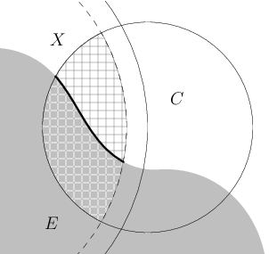
The constants in 2.3 are not important and one could also impose a stronger bound on the diameter of the balls $C\in\mathcal{C}$ for $\lambda$ near 1.

Note that the following 2.4 addresses the reduced boundary $\partial^{*}{E}$ and not the measure theoretic boundary $\partial_{*}{E}$.

This is a slightly more precise version of ${\mathrm{M}}f\geq f$ almost everywhere for characteristic functions.

References

- [1] J. M. Aldaz, L. Colzani, and J. Pérez Lázaro. Optimal bounds on the modulus of continuity of the uncentered Hardy-Littlewood maximal function. J. Geom. Anal., 22(1):132–167, 2012.
- [2] J. M. Aldaz and J. Pérez Lázaro. Functions of bounded variation, the derivative of the one dimensional maximal function, and applications to inequalities. Trans. Amer. Math. Soc., 359(5):2443–2461, 2007.
- [3] J. M. Aldaz and J. Pérez Lázaro. Boundedness and unboundedness results for some maximal operators on functions of bounded variation. J. Math. Anal. Appl., 337(1):130–143, 2008.
- [4] Anders Björn and Jana Björn. Nonlinear potential theory on metric spaces, volume 17 of EMS Tracts in Mathematics. European Mathematical Society (EMS), Zürich, 2011.
- [5] Stephen M. Buckley. Is the maximal function of a Lipschitz function continuous? Ann. Acad. Sci. Fenn. Math., 24(2):519–528, 1999.
- [6] Emanuel Carneiro, Renan Finder, and Mateus Sousa. On the variation of maximal operators of convolution type II. Rev. Mat. Iberoam., 34(2):739–766, 2018.
- [7] Emanuel Carneiro and Kevin Hughes. On the endpoint regularity of discrete maximal operators. Math. Res. Lett., 19(6):1245–1262, 2012.
- [8] Emanuel Carneiro and José Madrid. Derivative bounds for fractional maximal functions. Trans. Amer. Math. Soc., 369(6):4063–4092, 2017.
- [9] Emanuel Carneiro, José Madrid, and Lillian B. Pierce. Endpoint Sobolev and BV continuity for maximal operators. J. Funct. Anal., 273(10):3262–3294, 2017.
- [10] Emanuel Carneiro and Diego Moreira. On the regularity of maximal operators. Proc. Amer. Math. Soc., 136(12):4395–4404, 2008.
- [11] Emanuel Carneiro and Benar F. Svaiter. On the variation of maximal operators of convolution type. J. Funct. Anal., 265(5):837–865, 2013.
- [12] Lawrence C. Evans and Ronald F. Gariepy. Measure theory and fine properties of functions. Textbooks in Mathematics. CRC Press, Boca Raton, FL, revised edition, 2015.
- [13] Piotr Hajłasz. Jyväskylä lectures on Sobolev spaces. http://www.pitt.edu/~hajlasz/Notatki/jyv-98b.pdf.
- [14] Piotr Hajłasz and Jan Malý. On approximate differentiability of the maximal function. Proc. Amer. Math. Soc., 138(1):165–174, 2010.
- [15] Piotr Hajłasz and Jani Onninen. On boundedness of maximal functions in Sobolev spaces. Ann. Acad. Sci. Fenn. Math., 29(1):167–176, 2004.
- [16] Toni Heikkinen, Juha Kinnunen, Janne Korvenpää, and Heli Tuominen. Regularity of the local fractional maximal function. Ark. Mat., 53(1):127–154, 2015.
- [17] Juha Kinnunen. The Hardy-Littlewood maximal function of a Sobolev function. Israel J. Math., 100:117–124, 1997.
- [18] Juha Kinnunen, Riikka Korte, Nageswari Shanmugalingam, and Heli Tuominen. Lebesgue points and capacities via the boxing inequality in metric spaces. Indiana Univ. Math. J., 57(1):401–430, 2008.
- [19] Juha Kinnunen and Peter Lindqvist. The derivative of the maximal function. J. Reine Angew. Math., 503:161–167, 1998.
- [20] Juha Kinnunen and Eero Saksman. Regularity of the fractional maximal function. Bull. London Math. Soc., 35(4):529–535, 2003.
- [21] Ondřej Kurka. On the variation of the Hardy-Littlewood maximal function. Ann. Acad. Sci. Fenn. Math., 40(1):109–133, 2015.
- [22] Hannes Luiro. The variation of the maximal function of a radial function. Ark. Mat., 56(1):147–161, 2018.
- [23] Hannes Luiro and José Madrid. The Variation of the Fractional Maximal Function of a Radial Function. arXiv e-prints, page arXiv:1710.07233, October 2017.
- [24] José Madrid. Sharp inequalities for the variation of the discrete maximal function. Bull. Aust. Math. Soc., 95(1):94–107, 2017.
- [25] João P. G. Ramos, Olli Saari, and Julian Weigt. Weak differentiability for fractional maximal functions of general functions on domains. arXiv e-prints, page arXiv:1909.04375, September 2019.
- [26] Hitoshi Tanaka. A remark on the derivative of the one-dimensional Hardy-Littlewood maximal function. Bull. Austral. Math. Soc., 65(2):253–258, 2002.