Graph Convolutional Subspace Clustering: A Robust Subspace Clustering Framework for Hyperspectral Image
Abstract
Hyperspectral image (HSI) clustering is a challenging task due to the high complexity of HSI data. Subspace clustering has been proven to be powerful for exploiting the intrinsic relationship between data points. Despite the impressive performance in the HSI clustering, traditional subspace clustering methods often ignore the inherent structural information among data. In this paper, we revisit the subspace clustering with graph convolution and present a novel subspace clustering framework called Graph Convolutional Subspace Clustering (GCSC) for robust HSI clustering. Specifically, the framework recasts the self-expressiveness property of the data into the non-Euclidean domain, which results in a more robust graph embedding dictionary. We show that traditional subspace clustering models are the special forms of our framework with the Euclidean data. Basing on the framework, we further propose two novel subspace clustering models by using the Frobenius norm, namely Efficient GCSC (EGCSC) and Efficient Kernel GCSC (EKGCSC). Both models have a globally optimal closed-form solution, which makes them easier to implement, train, and apply in practice. Extensive experiments on three popular HSI datasets demonstrate that EGCSC and EKGCSC can achieve state-of-the-art clustering performance and dramatically outperforms many existing methods with significant margins.
Index Terms:
Hyperspectral Image Clustering, Graph Convolutional Networks, Subspace Clustering, Kernel MethodI Introduction
Hyperspectral images (HSIs) acquired by remote sensors contain rich spectral and spatial information, which enables us to accurately recognize the region of interest. Over the past decade, HSIs have been widely applied to various fields, ranging from geological exploration, marine monitoring, military reconnaissance to medical imaging and forensics [1, 2, 3].
HSI classification, which aims to classify every pixel with a certain label, is the foundation for the application of HSI [3, 4]. The most commonly used HSI classification method is the supervised classification [5, 6] based on label information. In recent years, the supervised HSI classification has made great progress. For several popular HSI datasets, such as Indian Pines, Salinas and Pavia University images [1, 7], the supervised methods have achieved excellent classification accuracy. Particularly, deep learning models [8, 1, 9, 10], such as Convolutional Neural Networks (CNNs) [11, 12], have extremely narrowed the gap between human and machine. Unfortunately, the supervised method typically requires a large amount of labeled data, which cannot be satisfied in HSI scenarios due to the high cost of labeling training data. Furthermore, the supervised methods are difficult to deal with unknown objects, since they are modeled by the known classes.
To avoid manual data annotation, many works have dedicated to developing unsupervised HSI classification methods namely HSI clustering. Instead of using the label information, the HSI clustering aims to find the intrinsic relationship between data points and automatically determine labels in an unsupervised manner [13]. The key to the HSI clustering is to measure the similarity between data points [14]. Traditional clustering methods, e.g., K-means [15], frequently use the pair-wise distance as the similarity measurement, such as the Euclidean distance. Owing to the mixed pixel and the redundant band problem [16, 17], these methods often suffer from unreliable measurement and making the HSI clustering in great challenges. Compared with the supervised classification, there are quite fewer studies on the HSI clustering [18] and they are usually uncompetitive in terms of accuracy.
Recently, subspace clustering [19] has drawn increasing attention in the HSI clustering [20, 21, 22, 23, 24] due to its ability to handle high-dimensional data and its reliable performance. Technically, the subspace clustering seeks to express the data points as a linear combination of a self-expressive dictionary in the same subspace [25]. The subspace clustering model typically consists of two steps, i.e., self-representation [26] and Spectral Clustering (SC) [24]. To improve the performance of the subspace clustering, many works have devoted to constructing a robust affinity matrix by using various techniques. For example, Sparse Subspace Clustering (SSC) [27] uses an -norm to encourage a sparse affinity matrix, while Low Rank Subspace Clustering (LRSC) [28] adopts a nuclear norm to enforce the affinity matrix to be low-rank. By considering the spectral and spatial properties of HSIs, Zhang et al. proposed a Spectral–Spatial Sparse Subspace Clustering (S4C) [23]. Kernel subspace clustering [29] was proposed as the nonlinear extension of the subspace clustering model by implicitly mapping data into higher kernel space. In [21], an improved kernel subspace clustering was applied to the HSI clustering.
However, the previous subspace clustering models are based on the Euclidean data and often ignore the inherent graph structure contained in the data points. On the one hand, the data points are usually corrupted by noise or can have entries with large errors. On the other hand, although manifold regularization is useful to incorporate graph information into the subspace clustering, such as graph regularized LRSC [30, 31], it usually needs to add an additional regularization term and a tradeoff parameter. The recent development of Graph Neural Networks (GNNs) [32, 33, 34] generalizes the powerful CNNs in dealing with the Euclidean data to modeling the graph-structured data. This allows us to revisit traditional problems with GNNs [35, 36]. However, the subspace clustering that combines graph learning has not attracted too much attention.
To learn graph embedding and affinity, simultaneously, in this paper, we present a Graph Convolutional Subspace Clustering (GCSC) framework that recasts the traditional subspace clustering into the non-Euclidean domain. Specifically, the GCSC framework calculates the self-representation coefficients of the subspace clustering by leveraging a graph convolutional self-representation model combining both graph and feature information. As a result, the proposed framework can circumvent noise data and tends to produce a more robust affinity than the traditional subspace clustering models. Visually, an intuitive description about the motivation of GCSC is illustrated in Fig. 1.
To sum up, the main contributions of this work are:
- 1.
A robust subspace clustering framework called GCSC is developed for the HSI clustering in which the subspace clustering is recasted into the non-Euclidean domain. Particularly, the traditional subspace clustering can be viewed as the special form of the proposed framework.
- 2.
Based on the Frobenius norm, two novel and efficient subspace clustering models are proposed under the GCSC framework. We refer to them as Efficient GCSC (EGCSC) and Efficient Kernel GCSC (EKGCSC), respectively. Both EGCSC and EKGCSC have a closed-form solution, making them easier to implement, train, and apply in practice.
- 3.
Our experimental results on several HSI datasets show that the proposed subspace clustering models are effectively better than many existing clustering methods for the HSI clustering. The successful attempt of GCSC offers an alternative orientation for unsupervised learning.
The rest of the paper is structured as follows. We first briefly review the subspace clustering, graph convolutional networks, and HSI clustering in Section II. Secondly, we describe the details of the developed GCSC framework and its two implementations in Section III. In section IV, we give extensive experimental results and empirical analysis. Finally, we conclude with a summary and final remarks in Section V.
II Preliminaries and Related Work
II-A Notations
Throughout this paper, boldface lowercase italics symbols (e.g., ), boldface uppercase roman symbols (e.g., ), regular italics symbols (e.g., ), and calligraphy symbols (e.g., ) denote vectors, matrices, scalars, and sets, respectively. A graph is represented as , where denotes the node set of the graph with and , indicates the edge set with , and stands for an adjacency matrix. We define the diagonal degree matrix of the graph as , where . The graph Laplacian is defined as , and its normalized version is given by . In this paper, denotes the transpose of matrix and denotes an identity matrix with the size of . The Frobenius norm of a matrix is defined as and the trace of a matrix is denoted as .
II-B Subspace Clustering Models
Let be a collection of data points drawn from a union of linear or affinity subspaces , where , , and denote the number of data points, features, and subspaces, respectively. The subspace clustering model for the given data set is defined as the following self-representation problem [27, 31]:
| (1) |
where denotes the self-expressive coefficient matrix and enforces the diagonal elements of to be zero so that the trivial solutions are avoided. denotes a -norm of matrix , e.g., (SSC) [27]), and (-SSC [22]) .
In the SSC model, the self-expressive coefficient matrix is assumed to be sparse and the self-representation problem is often formulated as
| (2) |
Here, the -norm tends to produce a sparse coefficient matrix. By using a nuclear norm, LRSC [37, 38, 31] reformulates the self-expressiveness property of data as
| (3) |
where and denote the nuclear norm and -norm of a matrix. LRSC has been proven to be effective to incorporate the global structure of data. Furthermore, subspace clustering can use to model corrupted data, i.e., where is arbitrary noise.
The above problems can be efficiently solved by using convex optimization methods, such as Alternating Direction Method of Multipliers (ADMM) [19, 39]. Once the coefficient matrix is found, the subspace clustering seeks to segment an affinity matrix by Spectral Clustering (SC) method [24].

II-C Graph Convolutional Networks
There is an increasing interest in generalizing convolutions to the graph domain [32, 40]. The recent development of GNNs that allows to efficiently approximate convolution on graph-structured data. GNNs can typically divide into two categories [34, 33]: spectral convolutions, which perform convolution by transforming node representations into the spectral domain using the graph Fourier transform or its extensions, and spatial convolutions, which perform convolution by considering node neighborhoods. Unless otherwise specified, the graph convolution involved in this paper is the spectral convolution.
One of the most representative graph convolution models is the Graph convolutional networks (GCN) developed by Kift et al. [36]. GCN simplifies the spectral convolution by approximating spectral filters with the -order Chebyshev polynomials and setting the largest eigenvalue of the normalized graph Laplacian to . Formally, GCN defines spectral convolution over a graph as follows:
| (4) |
Here, is an adjacency matrix with self-loops, denotes the degree matrix of nodes whose elements are given by , denotes a trainable parameter matrix, and is a nonlinear activation function. Specifically, GCN takes a node feature matrix and an adjacency matrix as inputs, and produce a graph embedding , where is the output dimension.
GCN is originally developed for semi-supervised node classification. By stacking several graph convolution layers, GCN is possible to learn deeper graph representation. Similar to traditional deep neural networks, GCN can be easily trained using gradient descent methods. In different tasks, the GCN models allow many traditional problems to be revised in the non-Euclidean domain.
II-D HSI Clustering
Although supervised methods have achieved great success in HSI classification [5, 9], they are limited by the lack of sufficient labeled data. To avoid data annotation, HSI clustering has attracted increasing attention. HSI clustering is based on the fact that the same land-cover object often shows similar spectral curves. The traditional centroid based clustering methods, such as K-means [41] and fuzzy c-means (FCM) [42], are widely used and easy to implement. However, this kind of method is sensitive to the random initialization state and thus their clustering results are hard to reproduce [18].
Due to the stable performance, subspace clustering is frequently-used for HSI clustering. Zhang et al. [22, 21, 20, 23] have successfully applied various subspace clustering methods to the HSI clustering, including Spectral–Spatial Sparse Subspace Clustering (S4C) [23], Kernel Sparse Subspace Clustering [21], Joint Sparsity Based Sparse Subspace Clustering (JSSC) [20], and so on. It is benefited from the ability to exploit the intrinsic structure of data, subspace clustering has achieved impressive performance. In recently, evolutionary optimization based clustering method has attracted increasing interests, e.g., evolutionary multiobjective optimization based HSI clustering [43, 44]. It is well known that the evolutionary algorithm is powerful to search the globally optimal solution but it often results in huge computational cost [45, 46, 47, 48].
It has been proven to be effective to improve HSI clustering performance by utilizing spectral and spatial information, simultaneously. In [18], Zhang et al. developed a state-of-the-art HSI clustering method called Robust Manifold Matrix Factorization (RMMF) clustering by combining HSI dimensionality reduction and data clustering, simultaneously. Kong et al. [49] proposed an Unsupervised Broad Learning (UBL) clustering method that combines clustering with broad representation learning. In our recent work [50], we proposed a deep subspace clustering method for the HSI clustering, which further demonstrates the potential of combining clustering models with feature learning.
III Methodology
In this section, we first introduce the proposed Graph Convolutional Subspace Clustering (GCSC) framework. Then, we provide the details of two novel subspace clustering models based on the framework, i.e., Efficient Graph Convolutional Subspace Clustering (EGCSC) and Efficient Kernel Graph Convolutional Subspace Clustering (EKGCSC). We illustrate a schematic representation of the proposed framework in Fig. 2 and more details are given in the following subsections.
III-A Graph Convolutional Subspace Clustering Framework
Inspired by the recent development of GCNs, we present a novel subspace clustering framework by incorporating graph embedding into subspace clustering. We refer to the framework as GCSC. The goal of the GCSC framework is to utilize graph convolution to learn a robust affinity. For this purpose, we first modify the traditional self-representation as follows:
| (5) |
Here, is the self-representation coefficient matrix and denotes the normalized symmetrical Laplacian matrix with self-loops. Notably, can be treated as a special linear graph convolution operation (or a special graph auto-encoder) parameterized by . We call Eq. (5) graph convolutional self-representation.
Parallel to traditional subspace clustering models, the GCSC framework can be rewritten as
| (6) |
where and denote any appropriate matrix norm, such as and nuclear norm, and is a tradeoff coefficient. It is easy to prove that the traditional subspace models are the special cases of our framework, i.e., the traditional subspace models depend only on data features. For example, when is the Frobenius norm and , Eq. (6) becomes the extension of the classical SSC [27], while is norm and is the nuclear norm, Eq. (6) degenerates to LRSC [28, 38]. Eq. (6) can be effectively solved by the same method adopted in the traditional subspace clustering. Once the self-representation coefficient matrix is obtained, SC can be used to generate the clustering results.
III-B Efficient GCSC
Basing on the proposed framework, we present the first novel subspace clustering model, namely Efficient GCSC (EGCSC), by setting both and to be the Frobenius norm. Formally, we formulate the EGCSC model as
| (7) |
In [51], Pan et al. have proven that the Frobenius norm will not result in trivial solutions even without constraint . This leads to a dense self-representation coefficient matrix and can be denoted as an efficient closed-form solution. The solution is given by
Having obtained , we can use it to construct an affinity matrix for the SC. However, there is no globally-accepted solution for this step in the literature. Most existing works typically compute the affinity matrix by or . In this paper, we use the heuristic adopted by Efficient Dense Subspace Clustering (EDSC) [51] to enhance the block-structure, which is proved beneficial for clustering accuracy. The pseudocode of the EGCSC is given in Algorithm 1.
III-C Efficient Kernel GCSC
We have proposed the EGCSC method. However, the EGCSC model is essentially modeled on linear subspaces. Due to the complexity and nonlinearity of HSI, a large number of works have demonstrated that nonlinear models will yield better performance than their linear counterparts. In this subsection, we provide a nonlinear extension of EGCSC by using the kernel trick. The extension is referred to as Efficient Kernel GCSC (EKGCSC).
Let be a mapping from the input space to the reproducing kernel Hilbert space . We define a positive semidefinite kernel Gram matrix as
| (9) |
where denotes the kernel function. In this paper, the Gaussian kernel is used, i.e., , where is the parameter of the Gaussian kernel function. Formally, the EKGCSC model is expressed as
| (10) |
By using kernel trick, Eq. (10) can be equivalently rewritten as
| (11) |
The above problem can be solved by calculating the partial derivative with respect to and set it to be zero (see Appendix section VI). The closed-form solution of EKGCSC is given by
| (12) |
The EKGCSC model explicitly maps the original data points onto a higher-dimensional space, and thus makes a linearly inseparable problem to be a separable one. We use a manner that is similar to EGCSC to construct the affinity matrix and obtain the final clustering results by SC. The pseudocode of EKGCSC is given in Algorithm 2.
III-D HSI Clustering Using The GCSC Models
We use the proposed GCSC models for HSI clustering. Two essential issues need to be tackled before using the GCSC models. First, HSI data often includes many spectral bands with lots of redundancy, and thus using only spectral features is hard to achieve good performance. Second, the GCSC models are based on the graph-structured data, and however, HSI is typically a Euclidean data.
To remedy the first issue, the following procedures are employed. We first use Principle Component Analysis (PCA) to reduce the spectral dimensionality by preserving the top PCs. On the one hand, PCA reduces the redundant information contained in HSI data. On the other hand, it increases computational efficiency when model training. To take spectral and spatial information consideration, simultaneously, we represent every data point by extracting 3D patches. Specifically, every data point is represented by the center pixel and its neighboring pixels. The manner is widely adopted in different HSI spectral-spatial classification methods [2, 7, 9].
For the second issue, we construct a -nearest neighbor (kNN) graph to represent the graph structure of the data points. Specifically, each data point is viewed as a node over the graph and the nearest neighbors of consists of the edge relationship. The adjacent matrix of a kNN graph is defined by
| (13) |
where indicates the nearest neighbors of . The neighborhood relationship is obtained by computing the Euclidean distance.
III-E Remarks on The Proposed GCSC
In this subsection, we provide a deeper insight into the GCSC framework from the following viewpoints. Let be the graph embedding, thus GCSC can be rewritten as
| (14) |
From the viewpoint of sparse representation, GCSC aims to use a self-expressive dictionary matrix to reconstruct the original data. Since considers the global structure information, those noise points will be eliminated and a clear dictionary can be obtained, which is beneficial for producing a robust affinity matrix. It can be seen from Fig. 3, the resulting shows better clustering characteristics than the original . It can be further explained from the viewpoint of graph representation learning. Graph convolution essentially is a special form of the Laplacian smoothing [35], which combines the features of a node and its nearby neighbors. The operation makes the features of the node in the same cluster similar, thus greatly easing the clustering task.
The main differences between the GCSC model and the traditional subspace model are as follows. First, GCSC is built in the non-Euclidean domain. Under the GCSC framework, the traditional subspace clustering models can be considered as special cases in the Euclidean domain. Second, GCSC incorporates the graph structure via graph convolution, while the traditional subspace clustering models do this by manifold regularization. Therefore, GCSC exploits graph information using a more straightforward way.
| Datasets | SalinasA | Indian Pines | Pavia University |
|---|---|---|---|
| Pixels | 8386 | 8570 | 140150 |
| Channels | 204 | 200 | 103 |
| Clusters | 6 | 4 | 8 |
| Samples | 5348 | 4391 | 6445 |
| Sensor | AVIRIS | AVIRIS | ROSIS |
IV Experiments
| Method | EGCSC | EKGCSC | |||
|---|---|---|---|---|---|
| SalinasA | 100 | 30 | 100 | 30 | 0.2 |
| Indian Pines | 100 | 30 | 100000 | 30 | 6 |
| Pavia University | 1000 | 20 | 60000 | 30 | 100 |
In this section, we extensively evaluate the clustering performance of the proposed clustering methods on three frequently used HSI datasets. The source codes of EGCSC and EKGCEC are released at https://github.com/AngryCai/GraphConvSC.
IV-A Setup
IV-A1 Datasets and Preprocessing
We conduct experiments on three real HSI images acquired by AVIRIS and ROSIS sensors, i.e., Salinas, Indian Pines, and Pavia University. For computational efficiency, we separately take a sub-scene of these datasets for evaluation as it is done in [30, 53, 49]. Specifically, these sub-scenes are located within the original scenes at , , and , respectively. Notice that the sub-scene taken from the Salinas dataset is also known as the SalinasA dataset. The details of the three datasets are summarized in Table I.
In data preprocessing, we perform PCA to reduce spectral bands into by preserving at least of the cumulative percentage of variance. We construct spectral-spatial samples by setting neighborhood size to be for all the datasets. All data points are standardized by scaling into before clustering.
IV-A2 Evaluation Metrics
Three popular metrics [23, 18, 49] are used to evaluate the clustering performance of clustering models, i.e., Overall Accuracy (OA), Normalized Mutual Information (NMI), and Kappa coefficient (Kappa). These metrics range in , and the higher the scores are, the more accurate the clustering results are achieved. Besides, to evaluate the computational complexity of our models, running time is compared in the experiment.
IV-A3 Compared Methods
We compare the proposed methods with several existing HSI clustering methods, including traditional clustering methods and state-of-the-art methods. Specifically, the compared traditional clustering methods contain Spectral Clustering (SC) [24], Sparse Subspace Clustering (SSC) [27], Efficient Dense Subspace Clustering (EDSC) [51], Low Rank Subspace Clustering (LRSC) [37], and -norm based SSC (-SSC) [22]. The compared state-of-the-art HSI clustering methods are Spectral-Spatial Sparse Subspace Clustering (S4C) [23], Unsupervised Broad Learning (UBL) clustering [49], and Robust Manifold Matrix Factorization (RMMF) [18].
For these HSI clustering methods, i.e., -SSC, S4C, UBL, and RMMF, we follow their settings reported in the corresponding literature. The hyper-parameters of EGCSC and EKGCSC are given in Table II. All the compared methods are implemented with Python 3.5 running on an Intel Xeon E5-2620 2.10 GHz CPU with 32 GB RAM.
| Data | Metric | SC [24] | SSC [27] | LRSC [37] | -SSC [22] | S4C [23] | UBL [49] | RMMF [18] | EDSC [51] | EGCSC | EKGCSC |
|---|---|---|---|---|---|---|---|---|---|---|---|
| SaA. | OA | 0.6806 | 0.7666 | 0.5613 | 0.6412 | 0.8631 | 0.9142 | 0.9820 | 0.8702 | 0.9985 | 1.0000 |
| NMI | 0.7464 | 0.7571 | 0.4242 | 0.6971 | 0.7977 | 0.8692 | 0.9483 | 0.9135 | 0.9949 | 1.0000 | |
| Kappa | 0.6002 | 0.7138 | 0.4487 | 0.5546 | 0.8312 | 0.8943 | 0.9775 | 0.8384 | 0.9981 | 1.0000 | |
| InP. | OA | 0.6841 | 0.4937 | 0.5142 | 0.6645 | 0.7008 | 0.6258 | 0.7121 | 0.7126 | 0.8483 | 0.8761 |
| NMI | 0.5339 | 0.2261 | 0.2455 | 0.3380 | 0.5445 | 0.6680 | 0.4985 | 0.4717 | 0.6422 | 0.6959 | |
| Kappa | 0.5055 | 0.2913 | 0.3145 | 0.5260 | 0.5825 | 0.4690 | 0.5609 | 0.5657 | 0.6422 | 0.8211 | |
| PaU. | OA | 0.7691 | 0.6146 | 0.4326 | 0.5842 | 0.6509 | 0.7083 | 0.7704 | 0.6175 | 0.8442 | 0.9736 |
| NMI | 0.6784 | 0.6545 | 0.3793 | 0.4942 | 0.7031 | 0.6874 | 0.7388 | 0.5750 | 0.8401 | 0.9529 | |
| Kappa | 0.8086 | 0.4886 | 0.2549 | 0.3687 | 0.5852 | 0.6533 | 0.6804 | 0.4250 | 0.7968 | 0.9653 |
IV-B Results
IV-B1 Quantitative Results
Table III gives the clustering performance comparison of different methods evaluated on SalinasA, Indian Pines, and Pavia University datasets. As can be seen from the results, the proposed GCSC methods achieve the best clustering performance and significantly outperform the other clustering methods in terms of OA, NMI, and Kappa. We can further find the following tendencies from the results.
First, equipped with graph convolution, the traditional subspace clustering models can achieve remarkable improvement compared with the traditional counterpart. For example, EGCSC is significantly better than EDSC. It signifies that the proposed GCSC framework is beneficial for subspace clustering. It can be further seen from Table III, few of the compared clustering methods can achieve OA. On the contrary, OAs yielded by the EGCSC and EKGCSC models are generally better than on all the datasets. Particularly, on the SalinasA dataset, EKGCSC achieves a perfect () clustering performance.
Second, EKGCSC outperforms EGCSC on all the three datasets. Due to the complexity of HSI, linear models often can not fully exploit the relationship among data points. By extending EGCSC into the nonlinear kernel space, EKGCSC’s performance can be dramatically enhanced. In other words, EKGCSC considers the nonlinear relationship between data points and makes the learned affinity matrix more robust. In the experiment, EKGCSC achieves , , and improvement on SalinasA, Indian Pines, and Pavia University datasets, respectively.
Third, the results obtained by EGCSC and EKGCSC are comparable with many supervised HSI classification methods [9, 5, 54]. Specifically, the EKGCSC model achieves , , and in terms of OA on the SalinasA, Indian Pines, and Pavia University datasets, respectively. The recent development of supervised HSI classification allows achieving excellent results. However, the unsupervised classification of HSI is still a challenging task. The state-of-the-art clustering performance of our methods bridges the gap between unsupervised HSI classification and supervised HSI classification.
IV-B2 Results Visualization


To visually observe the clustering results, we visualize the clustering maps of different clustering methods in Fig. 4-6. Since the source codes of S4C and UBL have not been released, their class maps are not included in the figures but it does not affect the analysis. Notice that the color of the same class may be variant in different class maps, which is because label values may be permuted by different clustering methods. Observed from Fig. 4, the class map obtained by EKGCSC on the SalinasA dataset is in complete agreement with the ground truth. For the Indian Pines and Pavia University datasets (i.e., Fig. 5 and Fig. 6), EKGCSC shows the best class maps that are closest to the ground truths. Compared with the other competitors, EGCSC shows better class maps. While the class maps obtained by the other methods ( e.g., SSC, LRSC, and EDSC) contain relatively more noisy points caused by misclassification. Briefly, the results demonstrate the effectiveness and superiority of the proposed GCSC framework.
IV-B3 Visualization of The Learned Affinity Matrix
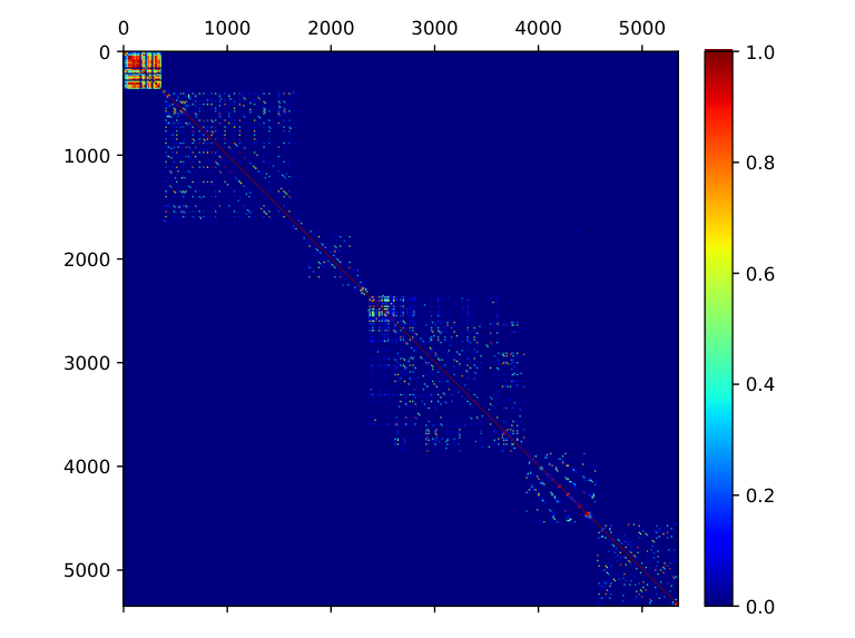

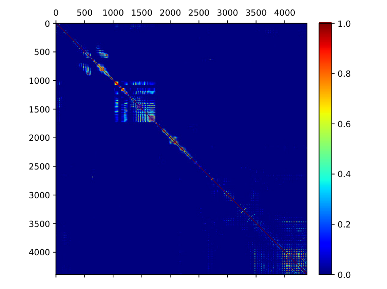
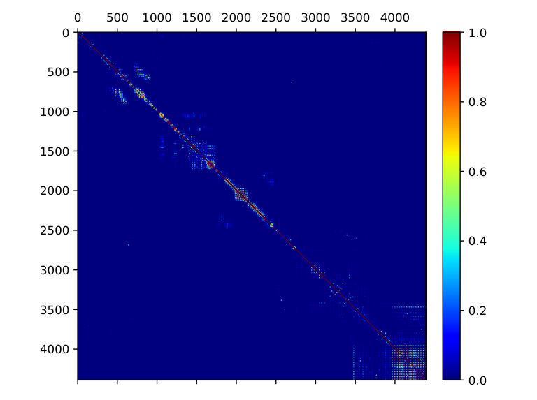


In Fig. 7, we visualize the affinity matrices learned by the EGCSC and EKGCSC models. For better presentation, we have re-ordered data points according to the ground truth before computing the affinity matrix. In the figures, each column or row of the affinity matrix denotes the self-representation coefficients that using all data points to represent the corresponding data point. Therefore, the larger the coefficient is, the more the corresponding data point contributes to the reconstruction. Ideally, if a group of data points belongs to the same cluster, then their self-representation coefficients to each other will be non-zero, otherwise, they will be zero. Thus, an ideal affinity matrix is block-diagonal. From Fig. 7 (a)-(f), we can observe that the obtained affinity matrices by both EGCSC and EKGCSC are sparse and have an apparent block-diagonal structure. Furthermore, EKGCSC shows better block-structure than EGCSC, which demonstrates that EKGCSC can more accurately explore the intrinsic relationships between data points and thus achieve better performance.
IV-B4 Impact of and
In this experiment, we investigate the impact of the two most important hyper-parameters involved in the GCSC framework, i.e., the regularization coefficient and the number of the nearest neighbors for the kNN graph. We set in the range of for SalinasA and Indian Pines datasets, and for Pavia University dataset. For clarity, we take into account for plotting. For all datasets, we let vary from to with an interval of . The results are shown in Fig. 8. It can be seen that has a significant impact on clustering performance. We can further observe a tendency, i.e., the clustering performance will increase as increased. By contrast, both EGCSC and EKGCSC are insensitive to . However, when is too large, graph convolution will result in an over-smoothing problem. That is, the graph embedding of all the data points will become similar. Therefore, too large may negatively affect the clustering performance. According to the empirical study, we provide a group of the best hyper-parameter setting in Table II.
IV-B5 Impact of The Number of PCs
To empirically study the influence of the number of PCs, we perform the proposed methods with varying PCs from to . We show the results in Fig. 9. As shown in the figures, the clustering performance of the GCSC models increases with PCs, which is because more spectral information will be included when more PCs are considered. However, it does not always enhance model performance since more redundancy might be increased. For example, Fig. 9 (c) shows the best number of PCs is instead of . Although dimensionality reduction is an optional step in our framework, it achieves a good balance between the computational efficiency and model performance.
IV-B6 Comparison of Running Time
| Data | SC [24] | SSC [27] | LRSC [37] | -SSC [22] | S4C [23] | UBL [49] | RMMF [18] | EDSC [51] | EGCSC | EKGCSC |
|---|---|---|---|---|---|---|---|---|---|---|
| SaA. | 13.203 | 855.663 | 7030.710 | 4.717 | 9363.5 | 2509.68 | 9.448 | 42.762 | 92.951 | 131.485 |
| InP. | 8.587 | 653.998 | 3980.004 | 3.272 | 1567.9 | 104.90 | 1.494 | 24.093 | 69.366 | 99.052 |
| PaU. | 15.640 | 1022.382 | 15861.621 | 15.677 | 7398.3 | 237.44 | 4.310 | 98.533 | 124.333 | 264.649 |
We compare our methods with the other competitors in terms of running time. Table IV lists the running time of different clustering methods. Since EGCSC and EKGCSC have closed-form solutions without needing an iterative operation, they are significantly faster than SSC, LRSC, S4C, and UBL. Although SC, -SSC, and RMMF take less running time, they cannot achieve better performance than our methods. Compared with EDSC, both of our methods take relatively more running time, which is because the proposed GCSC framework needs to construct the graph from data points. Furthermore, EKGCSC needs to compute the kernel matrix, thus its running time will be increased compared with EGCSC. To sum up, our proposed EGCSC and EKGCSC models achieve a good balance between time cost and clustering accuracy.
V Conclusions
We have proposed a novel HSI clustering framework, termed as GCSC, based on introducing graph convolution into subspace clustering. The key to the proposed framework is to utilize a graph convolutional self-representation to incorporate the intrinsic structure information of data points. Traditional subspace clustering models can be treated as the special forms of the GCSC framework built on the Euclidean data. Benefiting from the graph convolution, the GCSC model tends to use a clear dictionary to learn a robust affinity matrix. We design two efficient subspace clustering models (i.e., EGCSC and EKGCSC) based on the proposed GCSC framework by using the Frobenius norm. The experimental results on three HSI data sets demonstrate that the proposed GCSC models can achieve state-of-the-art performance with significant margins compared with many existing clustering models. Particularly, the EKGCSC model achieves , , and clustering OA on SalinasA, Indian Pines, and Pavia University datasets, respectively.
The successful attempt of the GCSC model signifies that considering the intrinsic graph structure among data set is important for clustering, which offers an alternative orientation for unsupervised learning. The proposed GCSC framework also enables us to revisit traditional clustering models in the non-Euclidean domain. There are many promising ways to improve the GCSC model. For example, one can consider deep graph embedding into GCSC. These issues will be further studied in our future works.
VI Appendix
Proof:
The solution of EGCSC.
Let be the loss function of EGCSC and Eq. (7) can be rewritten as
| (15) |
According to the properties of matrix trace and matrix derivatives, the partial derivative of with respect to can be presented as
| (16) |
Let , we get
| (17) |
Finally, can be expressed as
| (18) |
Due to is positive semidefinite, its reversible always exists. ∎
Proof:
The solution of EKGCSC.
Similar to the above proof, the loss function of EKGCSC (Eq. (10)) can be expressed as
| (19) |
The partial derivative of with respect to is then given by
| (20) |
By setting , we finally get the optimal solution of as follows:
| (21) |
∎
Acknowlegment
The authors would like to thank the anonymous reviewers for their constructive suggestions and criticisms. We would also like to thank Prof. Lefei Zhang who provided the source codes of the RMMF algorithm.
References
- [1] P. Ghamisi, N. Yokoya, J. Li, W. Liao, S. Liu, J. Plaza, B. Rasti, and A. Plaza, “Advances in hyperspectral image and signal processing: A comprehensive overview of the state of the art,” IEEE Geoscience and Remote Sensing Magazine, vol. 5, no. 4, pp. 37–78, Dec 2017.
- [2] Y. Cai, X. Liu, and Z. Cai, “Bs-nets: An end-to-end framework for band selection of hyperspectral image,” IEEE Transactions on Geoscience and Remote Sensing, vol. 58, no. 3, pp. 1969–1984, 2020.
- [3] X. Liu, R. Wang, Z. Cai, Y. Cai, and X. Yin, “Deep multigrained cascade forest for hyperspectral image classification,” IEEE Transactions on Geoscience and Remote Sensing, vol. 57, no. 10, pp. 8169–8183, Oct 2019.
- [4] Y. Cai, Z. Dong, Z. Cai, X. Liu, and G. Wang, “Discriminative spectral-spatial attention-aware residual network for hyperspectral image classification,” in 2019 10th Workshop on Hyperspectral Imaging and Signal Processing: Evolution in Remote Sensing (WHISPERS), 2019, pp. 1–5.
- [5] P. Ghamisi, E. Maggiori, S. Li, R. Souza, Y. Tarablaka, G. Moser, A. De Giorgi, L. Fang, Y. Chen, M. Chi, S. B. Serpico, and J. A. Benediktsson, “New frontiers in spectral-spatial hyperspectral image classification: The latest advances based on mathematical morphology, markov random fields, segmentation, sparse representation, and deep learning,” IEEE Geoscience and Remote Sensing Magazine, vol. 6, no. 3, pp. 10–43, Sep. 2018.
- [6] A. Qin, Z. Shang, J. Tian, Y. Wang, T. Zhang, and Y. Y. Tang, “Spectral-spatial graph convolutional networks for semisupervised hyperspectral image classification,” IEEE Geoscience and Remote Sensing Letters, vol. 16, no. 2, pp. 241–245, Feb 2019.
- [7] M. Fauvel, Y. Tarabalka, J. A. Benediktsson, J. Chanussot, and J. C. Tilton, “Advances in spectral-spatial classification of hyperspectral images,” Proceedings of the IEEE, vol. 101, no. 3, pp. 652–675, March 2013.
- [8] S. Li, W. Song, L. Fang, Y. Chen, P. Ghamisi, and J. A. Benediktsson, “Deep learning for hyperspectral image classification: An overview,” IEEE Transactions on Geoscience and Remote Sensing, vol. 57, no. 9, pp. 6690–6709, Sep. 2019.
- [9] L. He, J. Li, C. Liu, and S. Li, “Recent advances on spectral-spatial hyperspectral image classification: An overview and new guidelines,” IEEE Transactions on Geoscience and Remote Sensing, vol. 56, no. 3, pp. 1579–1597, 2018.
- [10] Y. Cai, X. Liu, Y. Zhang, and Z. Cai, “Hierarchical ensemble of extreme learning machine,” Pattern Recognition Letters, 2018.
- [11] J. Gu, Z. Wang, J. Kuen, L. Ma, A. Shahroudy, B. Shuai, T. Liu, X. Wang, G. Wang, J. Cai, and T. Chen, “Recent advances in convolutional neural networks,” Pattern Recognition, vol. 77, pp. 354–377, 2018.
- [12] Y. LeCun, Y. Bengio, and G. Hinton, “Deep learning,” Nature, vol. 521, no. 7553, pp. 436–444, 2015.
- [13] W. Sun, L. Zhang, B. Du, W. Li, and Y. M. Lai, “Band selection using improved sparse subspace clustering for hyperspectral imagery classification,” IEEE Journal of Selected Topics in Applied Earth Observations and Remote Sensing, vol. 8, no. 6, pp. 2784–2797, June 2015.
- [14] J. Chang, G. Meng, L. Wang, S. Xiang, and C. Pan, “Deep self-evolution clustering,” IEEE Transactions on Pattern Analysis and Machine Intelligence, pp. 1–1, 2018.
- [15] J. Zhu, Z. Jiang, G. D. Evangelidis, C. Zhang, S. Pang, and Z. Li, “Efficient registration of multi-view point sets by k-means clustering,” Information Sciences, vol. 488, pp. 205 – 218, 2019.
- [16] P. Hu, X. Liu, Y. Cai, and Z. Cai, “Band selection of hyperspectral images using multiobjective optimization-based sparse self-representation,” IEEE Geoscience and Remote Sensing Letters, vol. 16, no. 3, pp. 452–456, March 2019.
- [17] M. Zeng, Y. Cai, Z. Cai, X. Liu, P. Hu, and J. Ku, “Unsupervised hyperspectral image band selection based on deep subspace clustering,” IEEE Geoscience and Remote Sensing Letters, pp. 1–5, 2019.
- [18] L. Zhang, L. Zhang, B. Du, J. You, and D. Tao, “Hyperspectral image unsupervised classification by robust manifold matrix factorization,” Information Sciences, vol. 485, pp. 154 – 169, 2019.
- [19] R. Vidal, “Subspace clustering,” IEEE Signal Processing Magazine, vol. 28, no. 2, pp. 52–68, March 2011.
- [20] S. Huang, H. Zhang, and A. Pižurica, “Joint sparsity based sparse subspace clustering for hyperspectral images,” in 2018 25th IEEE International Conference on Image Processing (ICIP), Oct 2018, pp. 3878–3882.
- [21] H. Zhai, H. Zhang, X. Xu, L. Zhang, and P. Li, “Kernel sparse subspace clustering with a spatial max pooling operation for hyperspectral remote sensing data interpretation,” Remote Sensing, vol. 9, no. 4, 2017.
- [22] H. Zhai, H. Zhang, L. Zhang, P. Li, and A. Plaza, “A new sparse subspace clustering algorithm for hyperspectral remote sensing imagery,” IEEE Geoscience and Remote Sensing Letters, vol. 14, no. 1, pp. 43–47, Jan 2017.
- [23] H. Zhang, H. Zhai, L. Zhang, and P. Li, “Spectral-spatial sparse subspace clustering for hyperspectral remote sensing images,” IEEE Transactions on Geoscience and Remote Sensing, vol. 54, no. 6, pp. 3672–3684, June 2016.
- [24] R. Wang, F. Nie, and W. Yu, “Fast spectral clustering with anchor graph for large hyperspectral images,” IEEE Geoscience and Remote Sensing Letters, vol. 14, no. 11, pp. 2003–2007, Nov 2017.
- [25] Q. Li, W. Liu, and L. Li, “Affinity learning via a diffusion process for subspace clustering,” Pattern Recognition, vol. 84, pp. 39 – 50, 2018.
- [26] P. Ji, T. Zhang, H. Li, M. Salzmann, and I. Reid, “Deep subspace clustering networks,” in Advances in Neural Information Processing Systems 30, I. Guyon, U. V. Luxburg, S. Bengio, H. Wallach, R. Fergus, S. Vishwanathan, and R. Garnett, Eds. Curran Associates, Inc., 2017, pp. 24–33.
- [27] E. Elhamifar and R. Vidal, “Sparse subspace clustering: Algorithm, theory, and applications,” IEEE Transactions on Pattern Analysis and Machine Intelligence, vol. 35, no. 11, pp. 2765–2781, Nov 2013.
- [28] R. Vidal and P. Favaro, “Low rank subspace clustering (lrsc),” Pattern Recognition Letters, vol. 43, pp. 47 – 61, 2014, iCPR2012 Awarded Papers.
- [29] V. M. Patel and R. Vidal, “Kernel sparse subspace clustering,” in 2014 IEEE International Conference on Image Processing (ICIP), 2014, pp. 2849–2853.
- [30] H. Zhai, H. Zhang, L. Zhang, and P. Li, “Laplacian-regularized low-rank subspace clustering for hyperspectral image band selection,” IEEE Transactions on Geoscience and Remote Sensing, pp. 1–18, 2018.
- [31] M. Yin, J. Gao, and Z. Lin, “Laplacian regularized low-rank representation and its applications,” IEEE Transactions on Pattern Analysis and Machine Intelligence, vol. 38, no. 3, pp. 504–517, March 2016.
- [32] J. Zhou, G. Cui, Z. Zhang, C. Yang, Z. Liu, L. Wang, C. Li, and M. Sun, “Graph neural networks: A review of methods and applications,” arXiv preprint arXiv:1812.08434, 2018.
- [33] Z. Wu, S. Pan, F. Chen, G. Long, C. Zhang, and P. S. Yu, “A comprehensive survey on graph neural networks,” IEEE Transactions on Neural Networks and Learning Systems, pp. 1–21, 2020.
- [34] Z. Zhang, P. Cui, and W. Zhu, “Deep learning on graphs: A survey,” IEEE Transactions on Knowledge and Data Engineering, pp. 1–1, 2020.
- [35] Q. Li, Z. Han, and X.-M. Wu, “Deeper insights into graph convolutional networks for semi-supervised learning,” in Thirty-Second AAAI Conference on Artificial Intelligence, 2018.
- [36] T. Kipf and M. Welling, “Semi-supervised classification with graph convolutional networks,” in International Conference on Learning Representations, 2017.
- [37] X. Zhu, S. Zhang, Y. Li, J. Zhang, L. Yang, and Y. Fang, “Low-rank sparse subspace for spectral clustering,” IEEE Transactions on Knowledge and Data Engineering, vol. 31, no. 8, pp. 1532–1543, Aug 2019.
- [38] G. Liu, Z. Lin, and Y. Yu, “Robust subspace segmentation by low-rank representation,” in Proceedings of the 27th International Conference on Machine Learning, 2010, pp. 663–670.
- [39] C. Lu, J. Feng, Z. Lin, T. Mei, and S. Yan, “Subspace clustering by block diagonal representation,” IEEE Transactions on Pattern Analysis and Machine Intelligence, vol. 41, no. 2, pp. 487–501, Feb 2019.
- [40] M. M. Bronstein, J. Bruna, Y. LeCun, A. Szlam, and P. Vandergheynst, “Geometric deep learning: Going beyond euclidean data,” IEEE Signal Processing Magazine, vol. 34, no. 4, pp. 18–42, July 2017.
- [41] J. A. Hartigan and M. A. Wong, “Algorithm as 136: A k-means clustering algorithm,” Journal of the Royal Statistical Society. Series C (Applied Statistics), vol. 28, no. 1, pp. 100–108, 1979.
- [42] T. Lei, X. Jia, Y. Zhang, S. Liu, H. Meng, and A. K. Nandi, “Superpixel-based fast fuzzy c-means clustering for color image segmentation,” IEEE Transactions on Fuzzy Systems, vol. 27, no. 9, pp. 1753–1766, 2019.
- [43] A. Paoli, F. Melgani, and E. Pasolli, “Clustering of hyperspectral images based on multiobjective particle swarm optimization,” IEEE Transactions on Geoscience and Remote Sensing, vol. 47, no. 12, pp. 4175–4188, 2009.
- [44] Y. Wan, Y. Zhong, A. Ma, and L. Zhang, “Multi-objective sparse subspace clustering for hyperspectral imagery,” IEEE Transactions on Geoscience and Remote Sensing, vol. 58, no. 4, pp. 2290–2307, 2020.
- [45] X. Fang, Y. Cai, Z. Cai, X. Jiang, and Z. Chen, “Sparse feature learning of hyperspectral imagery via multiobjective-based extreme learning machine.” Sensors, vol. 20, no. 5, p. 1262, 2020.
- [46] W. Gong and Z. Cai, “Parameter extraction of solar cell models using repaired adaptive differential evolution,” Solar Energy, vol. 94, pp. 209 – 220, 2013.
- [47] W. Gong, Y. Wang, Z. Cai, and L. Wang, “Finding multiple roots of nonlinear equation systems via a repulsion-based adaptive differential evolution,” IEEE Transactions on Systems, Man, and Cybernetics: Systems, pp. 1–15, 2018.
- [48] Y. Cai, Z. Cai, M. Zeng, X. Liu, J. Wu, and G. Wang, “A novel deep learning approach: Stacked evolutionary auto-encoder,” in 2018 International Joint Conference on Neural Networks (IJCNN), 2018, pp. 1–8.
- [49] Y. Kong, Y. Cheng, C. L. P. Chen, and X. Wang, “Hyperspectral image clustering based on unsupervised broad learning,” IEEE Geoscience and Remote Sensing Letters, pp. 1–5, 2019.
- [50] M. Zeng, Y. Cai, X. Liu, Z. Cai, and X. Li, “Spectral-spatial clustering of hyperspectral image based on laplacian regularized deep subspace clustering,” in IGARSS 2019 - 2019 IEEE International Geoscience and Remote Sensing Symposium, July 2019, pp. 2694–2697.
- [51] Pan Ji, M. Salzmann, and Hongdong Li, “Efficient dense subspace clustering,” in IEEE Winter Conference on Applications of Computer Vision, March 2014, pp. 461–468.
- [52] G. E. Hinton, “Visualizing high-dimensional data using t-sne,” Journal of Machine Learning Research, vol. 9, no. 2, pp. 2579–2605, 2008.
- [53] Y. Pan, Y. Jiao, T. Li, and Y. Gu, “An efficient algorithm for hyperspectral image clustering,” in ICASSP 2019 - 2019 IEEE International Conference on Acoustics, Speech and Signal Processing (ICASSP), May 2019, pp. 2167–2171.
- [54] L. Zhang, L. Zhang, and B. Du, “Deep learning for remote sensing data: A technical tutorial on the state of the art,” IEEE Geoscience and Remote Sensing Magazine, vol. 4, no. 2, pp. 22–40, 2016.