Modelling and Parameter Estimation for Discretely Observed Fractional Iterated Ornstein–Uhlenbeck Processes

Juan Kalemkerian Affiliation: Universidad de la República, Facultad de Ciencias.

Abstract

In this work we present how to model an observed time series by a FOU $(p)$ process. We will show that the FOU $(p)$ processes can be used to model a wide range of time series varying from short range dependence to long range dependence, with performance similar to the ARMA or ARFIMA models and in several cases outperforming them. Also, we extend the theoretical results for any FOU $(p)$ processes for the case in which the Hurst parameter is less than $1/2$ and we show theoretically and by simulations that under some conditions on $T$ and the sample size $n$ it is possible to obtain consistent estimators of the parameters when the process is observed in a discretized and equispaced interval $[0,T]$ . Lastly, we give a way to obtain explicit formulas for the auto-covariance function for any FOU $(p)$ and we present an application for FOU $(2)$ and FOU $(3)$ .

Keywords: fractional Brownian motion, fractional Ornstein-Uhlenbeck process, long memory processes. AMS: 62M10

1 Introduction

Frequently, the real time series data sets that can be found in the applications are measurements of a certain variable at equispaced intervals. The nature of many of these processes is in continuous time. Although there are many continuous time stochastic processes that can be used to model these situations, the discrete time models such as ARMA or ARFIMA remain the most popular for practitioners. In [13], the continuous time FOU $(p)$ processes are defined. The FOU $(p)$ are centred Gaussian stationary processes and are a particular case of more general processes defined in [1] when the functional defined in [1] are applied to a fractional Brownian motion. A FOU $(p)$ process has two parameters, $H$ and $\sigma$ , given by the fractional Brownian motion, and in [13] it is proved that $H$ gives information about the irregularity of the trajectories, because it is proved that (using a result of [8] about the relation between the variogram and the Hölder index of any Gaussian process) $H$ is the Hölder index of any FOU $(p)$ . Then it is possible to apply a procedure suggested in [9] to estimate $H$ and $\sigma$ in a consistent way. The FOU $(p)$ processes also contain other parameters that give information about the local dependence, which we called the $\lambda$ parameters. In [13] the theoretical properties are established and a method to estimate their parameters with their asymptotic behaviour was constructed. The estimation method and the asymptotic results for the $\lambda$ parameters were obtained under the assumption that the process is observed in the entire interval $[0,T]$ where $T$ goes to $\infty$ . This condition is unrealistic because in practice every sample has a finite number of observations. This difficulty will be resolved in the present paper. For $p\geq 2$ , the FOU $(p)$ processes have short range dependence, and when $p=1$ we have the fractional Ornstein–Uhlenbeck processes (FOU) defined in [6], which have long range dependence when $H>1/2$ . Also, the FOU $(p)$ processes have a continuity structure in the $\lambda$ parameters, which allows us to approximate an FOU process by a subfamily of FOU $(2)$ . Thus, the FOU $(p)$ processes can be viewed as a generalization of FOU processes and can be used to model both types of time series: short and long range dependence. In the present paper we will present a consistent way to estimate the $\lambda$ parameters when the process is viewed for $n$ equispaced observations within the interval $[0,T]$ . In Section 2, we give the definition of an FOU $\left(p\right)$ process, as defined in [13], and summarize the theoretical properties that established in [13] for $H>1/2$ . Also we will present a way to extend those properties to the case $H<1/2$ . In Section 3, we give a procedure to estimate all parameters at once in a consistent way, when the process is observed on an equispaced sample in $[0,T]$ . Also we include explicit formulas for the auto-covariance function of any FOU $(2)$ or FOU $(3)$ process, and present a way to obtain similar formulas for any FOU $(p)$ . In Section 4, we corroborate the theoretical results by simulations. We perform a small simulation study for FOU $(2)$ processes, give the estimations of the parameters and the standard deviations of all of them, for different sample sizes, different values of $T$ , and for different values of the true parameters. In Section 5, we show how we can model an observed time series by a FOU process. In Section 6 we apply the FOU $(p)$ processes to model three real data sets, two with short range dependence and the other with long range dependence, and compare the performance of these models with ARMA or ARFIMA models according to their predictive power. In Section 7 we make some final remarks. Our concluding remarks are given in Section 8. In Section 9, we present the proof of the results established in Section 3.

2 Definitions and properties

We start with the definition of a fractional Brownian motion and iterated Ornstein–Uhlenbeck process.

Definition 1.

A fractional Brownian motion with Hurst parameter $H\in\left(0,1\right]$ , is an almost surely continuous centred Gaussian process $\left\{B_{H}(t)\right\}_{t\in\mathbb{R}}$ such that its auto-covariance function is

\mathbb{E}\left(B_{H}(t)B_{H}(s)\right)=\frac{1}{2}\left(\left|t\right|^{2H}+\left|s\right|^{2H}-\left|t-s\right|^{2H}\right),\text{ \ }t,s\in\mathbb{R}.

We next give the definition of a fractional iterated Ornstein–Uhlenbeck processes of order $p$ (FOU $(p)$ ), as defined in [13].

Definition 2.

Suppose that $\left\{\sigma B_{H}(s)\right\}_{s\in\mathbb{R}}$ is a fractional Brownian motion with Hurst parameter $H$ and scale parameter $\sigma$ . Suppose further that $\lambda_{1},\lambda_{2},...,\lambda_{q}$ are distinct positive numbers and that $p_{1},p_{2},...,p_{q}\in\mathbb{N}$ are such that $p_{1}+p_{2}+...+p_{q}=p$ . Then a fractional iterated Ornstein–Uhlenbeck process of order $p$ is any process of the form

X_{t}:=T_{\lambda_{1}}^{p_{1}}\circ T_{\lambda_{2}}^{p_{2}}\circ....\circ T_{\lambda_{q}}^{p_{q}}(\sigma B_{H})(t)=\sum_{i=1}^{q}K_{i}\left(\lambda\right)\sum_{j=0}^{p_{i}-1}\binom{p_{i}-1}{j}T_{\lambda_{i}}^{\left(j\right)}(\sigma B_{H})(t),

where the numbers $K_{i}\left(\lambda\right)$ are defined by

K_{i}\left(\lambda\right)=K_{i}\left(\lambda_{1},\lambda_{2},...,\lambda_{q}\right):=\frac{1}{\prod\limits_{j\neq i}\left(1-\lambda_{j}/\lambda_{i}\right)}

(1)

and the operators $T_{\lambda_{i}}^{\left(j\right)}$ satisfy

T_{\lambda}^{(h)}(y)(t):=\int_{-\infty}^{t}e^{-\lambda(t-s)}\frac{\left(-\lambda\left(t-s\right)\right)^{h}}{h!}dy(s)\ \ \text{for}\ \ h=0,1,2,...

(2)

When $h=0$ we simply call this $T_{\lambda}$ , thus

T_{\lambda}(y)(t):=\int_{-\infty}^{t}e^{-\lambda(t-s)}dy(s).

(3)

Remark 1.

The equality between $T_{\lambda_{1}}^{p_{1}}\circ T_{\lambda_{2}}^{p_{2}}\circ....\circ T_{\lambda_{q}}^{p_{q}}$ and $\sum_{i=1}^{q}K_{i}\left(\lambda\right)\sum_{j=0}^{p_{i}-1}\binom{p_{i}-1}{j}T_{\lambda_{i}}^{\left(j\right)}$ is proved in [1].

Remark 2.

Observe that the composition $T_{\lambda_{1}}^{p_{1}}\circ T_{\lambda_{2}}^{p_{2}}\circ....\circ T_{\lambda_{q}}^{p_{q}}$ given in Definition 3 is commutative. Then, to avoid ambiguity in the estimation of the $\lambda$ we will assume that $\lambda_{1}<\lambda_{2}<...<\lambda_{q}$ .

Notation 1.

$\left\{X_{t}\right\}_{t\in\mathbb{R}}\sim\text{FOU }\left(\lambda_{1}^{\left(p_{1}\right)},\lambda_{2}^{\left(p_{2}\right)},...,\lambda_{q}^{\left(p_{q}\right)},\sigma,H\right),$ where $0<\lambda_{1}<\lambda_{2}<...<\lambda_{q}$ or more simply, $\left\{X_{t}\right\}_{t\in\mathbb{R}}\sim$ FOU $(p)$ .

Observe that the notation FOU $\left(\lambda_{1}^{\left(p_{1}\right)},\lambda_{2}^{\left(p_{2}\right)},...,\lambda_{q}^{\left(p_{q}\right)},\sigma,H\right)$ implies that the parameters $\lambda_{i}$ are distinct. Also, the notation FOU $(p)$ means that we have taken the composition of $T_{\lambda}$ $p$ times.

Remark 3.

When $p_{1}=p_{2}=...=p_{q}=1$ the process is equal to

X_{t}=T_{\lambda_{1}}\circ T_{\lambda_{2}}\circ...\circ T_{\lambda_{q}}(\sigma B_{H})(t)=\sum_{i=1}^{q}K_{i}\left(\lambda\right)T_{\lambda_{i}}(\sigma B_{H})(t)

(4)

and we write $\left\{X_{t}\right\}_{t\in\mathbb{R}}\sim$ FOU $\left(\lambda_{1},\lambda_{2},...,\lambda_{q},\sigma,H\right).$

Remark 4.

When $p=1$ , we obtain a fractional Ornstein–Uhlenbeck process (FOU $\left(\lambda,\sigma,H\right)$ ).

Remark 5.

Any FOU $\left(\lambda_{1}^{\left(p_{1}\right)},\lambda_{2}^{\left(p_{2}\right)},...,\lambda_{q}^{\left(p_{q}\right)},\sigma,H\right)$ , is a Gaussian, centred, and almost surely continuous process.

Any FOU $(p)$ has the property that almost all its trajectories are everywhere non differentiable. This fact will be used in Section 3 to obtain estimators of $H$ and $\sigma$ . The auto-covariance function of any $FOU\left(\lambda_{1},\lambda_{2},...,\lambda_{p},\sigma,H\right)$ is

\mathbb{E}\left(X_{0}X_{t}\right)=\frac{\sigma^{2}H}{2}\sum_{i=1}^{p}\frac{\lambda_{i}^{2p-2H-2}}{\prod\limits_{j\neq i}\left(\lambda_{i}^{2}-\lambda_{j}^{2}\right)}f_{H}(\lambda_{i}t)

(5)

where $p\geq 2$ and the function $f_{H}$ is defined by

f_{H}(x):=e^{-x}\left(\Gamma\left(2H\right)-\int_{0}^{x}e^{s}s^{2H-1}ds\right)+e^{x}\left(\Gamma\left(2H\right)-\int_{0}^{x}e^{-s}s^{2H-1}ds\right).

(6)

It is known that for $H>1/2$ , every FOU $\left(\lambda,\sigma,H\right)$ is a long memory process, Cheridito et al. [6], that is $\sum_{n=-\infty}^{+\infty}\left|\gamma\left(n\right)\right|=+\infty$ where $\gamma\left(n\right)=\mathbb{E}\left(X_{0}X_{n}\right).$ In [13] it is proved that if we compose at least two operators of the form $T_{\lambda}$ evaluated for a fractional Brownian motion, with Hurst parameter $H>1/2$ , we obtain a process $\left\{X_{t}\right\}_{t\in\mathbb{R}}$ that satisfies $\sum_{n=-\infty}^{+\infty}\left|\mathbb{E}\left(X_{0}X_{n}\right)\right|$ $<+\infty.$ Further, any FOU $(p)$ with $p\geq 2$ has short memory. Therefore, FOU $(p)$ has a short memory for $p\geq 2$ and a long memory for $p=1$ . Also, any FOU $(\lambda_{1},\lambda_{2},\sigma,H)$ goes to some FOU $(\lambda_{2},\sigma,H)$ when $\lambda_{1}$ goes to zero. Then, the FOU $(\lambda_{1},\lambda_{2},\sigma,H)$ for small values of $\lambda_{1}$ can be used to model both: a short range dependence and a long range dependence.

Observe that the $f_{H}$ are well defined for all $H\in\left[0,1\right].$ Pipiras and Taqqu ([17]) proved that when $H>1/2,$

\mathbb{E}\left(\int\int_{\mathbb{R}^{2}}f(u)g(v)dB_{H}(u)dB_{H}(v)\right)=H\left(2H-1\right)\int\int_{\mathbb{R}^{2}}f(u)g(v)\left|u-v\right|^{2H-2}dudv

(7)

holds for every $f$ and $g$ such that

\int\int_{\mathbb{R}^{2}}\left|f(u)g(v)\right|\left|u-v\right|^{2H-2}dudv<+\infty.

(8)

It is well known that (7) does not hold for $H\leq 1/2$ for every $f,g$ such that (8) holds. Neverthless, Cheridito et al. ([6]) have proved that the last equality remains valid for the exponential functions ( $f$ and $g$ ) that appear in the fractional iterated Ornstein–Uhlenbeck processes for values of $H\in\left(0,1/2\right)$ too. Therefore, we can follow the same line of proof as in [13] to prove that all the theoretical results obtained in Section 2 of [13] remain valid for all $H\in\left(0,1/2\right)\cup\left(1/2,1\right)$ .

3 Parameter estimation

Section 3 of [13] presents a procedure that allows estimating the parameters of any FOU $\left(p\right)$ in a consistent way. As with estimators $(\lambda,\sigma,H)$ proposed in [5] for the fractional Ornstein–Uhlenbeck process, this procedure has two steps. Firstly, we can estimate $\sigma$ and $H$ independently of the values of the $\lambda_{i}$ . Secondly, taking advantage for the explicit formula of the spectral density, and using $(\widehat{H},\widehat{\sigma})$ instead of $(H,\sigma)$ , we can estimate the $\lambda$ using Whittle estimators. To estimate $H$ and $\sigma$ it is enough to have an equispaced sample of $[0,T]$ and the results for consistency and asymptotic normality are valid for $H>1/2$ . To estimate the $\lambda$ it is necessary to observe the process over the whole interval $[0,T]$ .

In this section we present a way to extend the theoretical results to estimate $H$ and $\sigma$ for $H<1/2$ and we will show a procedure to consistently estimate the $\lambda$ parameters when the process is observed on an equispaced sample of $[0.T].$

3.1 Estimation of $H$ and $\sigma$

We start defining by filter of length $k+1$ and order $L$ .

Definition 3.

$a=\left(a_{0},a_{1},...,a_{k}\right)$ is a filter of length $k+1$ and order $L\geq 1$ if and only if the following conditions hold:

•

$\sum_{i=0}^{k}a_{i}i^{l}=0$ para todo $0\leq l\leq L-1.$
•

$\sum_{i=0}^{k}a_{i}i^{L}\neq 0.$

Observe that given $a,$ a filter of order $L$ and length $k+1$ , the new filter that we call $a^{2}$ and is defined by $a^{2}=\left(a_{0},0,a_{1},0,a_{2},0,...0,a_{k}\right)$ has order $L$ and length $2k+1$ . Now, we define the quadratic variation of a sample associated to a filter $a$ as follows.

Definition 4.

Given a filter $a$ of length $k+1$ and a sample $X_{1},X_{2},...,X_{n}$ , we define

V_{n,a}:=\frac{1}{n}\sum_{i=0}^{n-k}\left(\sum_{j=0}^{k}a_{j}X_{i+j}\right)^{2}.

The following theorem defines $\left(\hat{H},\hat{\sigma}\right)$ and summarizes their asymptotic properties.

Theorem 2 (Kalemkerian & León).

If $X_{\Delta},X_{2\Delta},....,X_{i\Delta},...,X_{n\Delta}=X_{T}$ is an equispaced sample of the process $\left\{X_{t}\right\}_{t\in\mathbb{R}}\sim$ FOU $\left(p\right)$ where $H>1/2$ , the filter $a$ is of order $L\geq 2$ and length $k+1$ , $\Delta_{n}=n^{-\alpha}$ for some $\alpha$ such that $0<\alpha<\frac{1}{2(2H-1)}$ and $T=n\Delta_{n}\rightarrow+\infty$ , as $n\rightarrow+\infty.$ Define

\widehat{H}=\frac{1}{2}\log_{2}\left(\frac{V_{n,a^{2}}}{V_{n,a}}\right),

(9)

\widehat{\sigma}=\left(\frac{-2V_{n,a}}{\Delta_{n}^{2\widehat{H}}\sum_{i=0}^{k}\sum_{j=0}^{k}a_{i}a_{j}\left|i-j\right|^{2\widehat{H}}}\right)^{1/2}.

(10)

Then

1.

$\left(\widehat{H},\widehat{\sigma}\right)\overset{c.s.}{\rightarrow}\left(H,\sigma\right).$
2.

$\sqrt{n}\left(\widehat{H}-H\right)\overset{w}{\rightarrow}N\left(0,\Gamma_{1}\left(H,\sigma,a\right)\right)$
3.

$\frac{\sqrt{n}}{\log n}\left(\widehat{\sigma}-\sigma\right)\overset{w}{\rightarrow}N\left(0,\Gamma_{2}\left(H,\sigma,a\right)\right)$

Remark 6.

Clearly the hypothesis $0<\alpha<\dfrac{1}{2(2H-1)}$ in Theorem 2 needs the condition that $H>1/2$ , but when $H<1/2$ , we can use Theorem 3 (iii) of Istas & Lang ([9]) in the case $s<1$ and follow the same proof taking $\alpha>1/2$ .

3.2 Estimation of the $\lambda$ parameters

If $X=\{X_{t}\}_{t\in\mathbb{R}}\sim$ $FOU(\lambda^{(p_{1})}_{1},\ldots,\lambda^{(p_{q})}_{q},\sigma,H)$ where $\sum_{i=1}^{q}p_{i}=p.$ It is proved in [13] that the spectral density of $X$ is

f^{(X)}(x)=\frac{\sigma^{2}\Gamma(2H+1)\sin(H\pi)|x|^{2p-1-2H}}{2\pi\prod_{i=1}^{q}(\lambda^{2}_{i}+x^{2})^{p_{i}}}.

(11)

If $H$ and $\sigma$ are known, taking advantage of the explicit knowledge of the spectral density and if the process is observed completely on $[0,T]$ , we can proceed as in [14] to estimate the rest of the parameters by using a modified Whittle contrast.

Theorem 3 (Kalemkerian & León).

Suppose given $\left\{X_{t}\right\}_{t\in\mathbb{R}}\sim FOU\left(\lambda_{1}^{\left(p_{1}\right)},\lambda_{2}^{\left(p_{2}\right)},...,\lambda_{q}^{\left(p_{q}\right)},\sigma,H\right)$ where $\sigma$ and $H$ are known. Suppose further that the true value of the parameter is $\lambda^{0}=\left(\lambda_{1}^{0},\lambda_{2}^{0},...,\lambda_{q}^{0}\right)$ $\in$ int $(\Lambda)$ where $\Lambda\subset\left\{\lambda\in\mathbb{R}^{q}\ :\ 0<\lambda_{1}<\lambda_{2}<...<\lambda_{q}\right\}$ is compact and the process is observed on $\left[0,T\right]$ for some $T>0.$ Define the following contrast process:

U_{T}\left(\lambda\right)=\frac{1}{4\pi}\int_{-\infty}^{+\infty}\left(\log f^{\left(X\right)}\left(x,\lambda\right)+\frac{I_{T}\left(x\right)}{f^{\left(X\right)}\left(x,\lambda\right)}\right)w\left(x\right)dx

where $f^{\left(X\right)}\left(x,\lambda\right)$ is the spectral density of the process given in (11), $I_{T}\left(x\right)$ is the periodogram of the second order

I_{T}\left(x\right)=\frac{1}{2\pi T}\left|\int_{0}^{T}X_{t}e^{-itx}dt\right|^{2}

and $w(x)=\frac{\left|x\right|}{1+\left|x\right|^{b}}$ where $b>2.$ Then $\widehat{\lambda}_{T}=\arg\min_{\lambda\in\Lambda}U_{T}\left(\lambda\right)$ satisfies

•

$\widehat{\lambda}_{T}\overset{P}{\rightarrow}\lambda^{0}$ when $T\rightarrow+\infty$ and
•

$\sqrt{T}\left(\widehat{\lambda}_{T}-\lambda^{0}\right)\overset{D}{\rightarrow}N_{q}\left(0,W_{1}^{-1}\left(\lambda^{0}\right)W_{2}\left(\lambda^{0}\right)W_{1}^{-1}\left(\lambda^{0}\right)\right)$ when $T\rightarrow+\infty$

where $N_{q}(.,.)$ denotes the $q-$ dimensional Gaussian law and the matrices $W_{1}\left(\lambda^{0}\right)$ and $W_{2}\left(\lambda^{0}\right)$ are defined by

W_{1}\left(\lambda\right)=\left(w_{ij}^{\left(1\right)}\left(\lambda\right)\right)_{i,j=1,...,q}\ \mbox{and}\ \ W_{2}\left(\lambda\right)=\left(w_{ij}^{\left(2\right)}\left(\lambda\right)\right)_{i,j=1,...,q}

where

	$\displaystyle w_{ij}^{\left(1\right)}\left(\lambda\right)$	$\displaystyle=$	$\displaystyle\frac{1}{4\pi}\int_{-\infty}^{+\infty}w(x)\frac{\partial}{\partial\lambda_{i}}\log f^{\left(X\right)}\left(x,\lambda\right)\frac{\partial}{\partial\lambda_{j}}\log f^{\left(X\right)}\left(x,\lambda\right)dx$
	$\displaystyle w_{ij}^{\left(2\right)}\left(\lambda\right)$	$\displaystyle=$	$\displaystyle\frac{1}{4\pi}\int_{-\infty}^{+\infty}w^{2}(x)\frac{\partial}{\partial\lambda_{i}}\log f^{\left(X\right)}\left(x,\lambda\right)\frac{\partial}{\partial\lambda_{j}}\log f^{\left(X\right)}\left(x,\lambda\right)dx.$

In the following theorem, we show the main theoretical result of this work that we will show that works well in the simulations (Section 4), and we use in the applications to real data (Section 6), that is, it is possible to take a discretized version of $U_{T}$ and $I_{T}$ , and using $\left(\widehat{H},\widehat{\sigma}\right)$ (given in (10) and (9)) instead of $(\sigma^{0},H^{0})$ , we obtain the same consistency result at the cost to adding a hypothesis about the speed with which $T_{n}$ tends to infinity and the need to change the function $w$ . In this way, we can estimate all the parameters consistenly in a FOU $(p)$ process observed in an equiespacied sample of $[0,T].$

Theorem 4.

Suppose $X_{\Delta},X_{2\Delta},X_{3\Delta},...,X_{n\Delta}$ is an equispaced sample in $\left[0;T\right]$ of some $\left\{X_{t}\right\}_{t\in\mathbb{R}}\sim$
FOU $\left(\lambda_{1}^{\left(p_{1}\right)},...,\lambda_{q}^{\left(p_{q}\right)},\sigma,H\right)$ where $p_{1}+p_{2}+...+p_{q}=p$ . Suppose further that $\left(\lambda,\sigma,H\right)\in\Lambda\times\left[\sigma_{1},\sigma_{2}\right]\times\left[h_{1},h_{2}\right]$ where $\sigma_{1}>0,$ $0<h_{1}<h_{2}<1,$ and $\Lambda\subset\left\{\lambda\in\mathbb{R}^{q}\ :\ 0<\lambda_{1}<\lambda_{2}<...<\lambda_{q}\right\}$ is compact. We call $\left(\lambda^{0},\sigma^{0},H^{0}\right)\in\overset{o}{\Lambda}\times\left(\sigma_{1},\sigma_{2}\right)\times\left(h_{1},h_{2}\right)$ the real vector of parameters. Define the weight function $w(x)=\frac{|x|^{a}}{1+|x|^{b}}$ where $a\geq 2p$ and $b\geq a+3$ .

Define the functions (for any fixed $T>0$ )

	$\displaystyle U_{T}\left(\lambda,\sigma,H\right)$	$\displaystyle=$	$\displaystyle\int_{0}^{T}h_{T}(x,\lambda,\sigma,H)dx\text{ and }$
	$\displaystyle U_{T}^{\left(n\right)}\left(\lambda,\sigma,H\right)$	$\displaystyle=$	$\displaystyle\frac{T}{n}\sum_{i=1}^{n}h_{T}^{\left(n\right)}\left(iT/n,\lambda,\sigma,H\right)$

where the functions $h_{T}$ and $h_{T}^{\left(n\right)}$ are defined by

h_{T}(x,\lambda,\sigma,H)=\frac{1}{2\pi}\left(\log f^{\left(X\right)}\left(x,\lambda,\sigma,H\right)+\frac{I_{T}(x)}{f^{\left(X\right)}\left(x,\lambda,\sigma,H\right)}\right)w(x),

h_{T}^{\left(n\right)}(x,\lambda,\sigma,H)=\frac{1}{2\pi}\left(\log f^{\left(X\right)}\left(x,\lambda,\sigma,H\right)+\frac{I_{T}^{\left(n\right)}(x)}{f^{\left(X\right)}\left(x,\lambda,\sigma,H\right)}\right)w(x)

where

I_{T}(x)=\frac{1}{2\pi T}\left|\int_{0}^{T}e^{itx}X_{t}dt\right|^{2}\text{ and }I_{T}^{\left(n\right)}(x)=\frac{T}{2\pi}\left|\frac{1}{n}\sum_{j=1}^{n}e^{\frac{ijTx}{n}}X_{\frac{jT}{n}}\right|^{2}

are the periodogram and the discretization of the periodogram respectively.

Define

	$\displaystyle\widehat{\lambda}_{T}$	$\displaystyle=$	$\displaystyle\arg\min_{\lambda\in\Lambda}U_{T}\left(\lambda,\sigma^{0},H^{0}\right),$		(12)
	$\displaystyle\widehat{\lambda}_{T}^{\left(n\right)}$	$\displaystyle=$	$\displaystyle\arg\min_{\lambda\in\Lambda}U_{T}^{\left(n\right)}\left(\lambda,\widehat{\sigma},\widehat{H}\right)$		(13)

where $\widehat{\sigma}$ and $\widehat{H}$ are defined by (10) and (9), respectively.

Suppose that the minimum of $U_{T}\left(\lambda,\sigma^{0},H^{0}\right)$ is reached at a unique point $\widehat{\lambda}_{T}.$

(A)

If $1/2<H<5/6$ , and if $T_{n}=n^{1-\alpha}$ where $\frac{3}{4}<\alpha<\min\{\frac{1}{2\left(2H-1\right)},1\}.$
(B)

If $H<1/2$ , and if $T_{n}=n^{1-\alpha}$ where $\max\{\frac{1}{H+1},\frac{3}{4}\}<\alpha<1.$

Then

\lim_{n\rightarrow+\infty}\widehat{\lambda}_{T_{n}}^{\left(n\right)}\overset{P}{=}\lambda^{0}.

Remark 7.

Conditions over $\alpha$ given in $(A)$ and $(B)$ , allows to affirm that as $n\rightarrow+\infty$ , $\frac{T_{n}^{4}}{n}\rightarrow 0$ and $\frac{T_{n}^{H+1}}{n^{H}}\rightarrow 0.$

Remark 8.

Results concerning to the convergence for the fractional Ornstein–Uhlenbeck processes are given for $1/2<H<3/4$ as can bee seen for example in [5] and [19]. In our case we have extend the theorem of convergence to $1/2<H<5/6.$

Corollary 1.

If $H$ and $\sigma$ are known, the result established in Theorem 4 is still valid, just changing the definition of $\widehat{\lambda}_{T}^{(n)}$ given in (13) to $\widehat{\lambda}_{T}^{(n)}=argmin_{\lambda\in\Lambda}U_{T}^{(n)}\left(\lambda,\sigma^{0},H^{0}\right).$

Remark 9.

The estimation of $H$ does not depend on the selection of $T$ , but the estimation of $\sigma$ depends on $T$ . Also, in the real data set considered in Section 5, we will see that $\hat{\sigma}$ varies considerably as a function of $T$ . The presence of the parameter $\sigma$ in the FOU $(p)$ model is simply as a multiplicative factor in the auto-covariance function. We show in Section 5 that we can choose previously a value of $\sigma$ (for example $\sigma=1$ ), and consider the FOU $(p)$ process as a model with parameters $H$ and $\lambda$ , and all the theoretical results about $\hat{H}$ and $\hat{\lambda}$ remain valid.

Remark 10.

The study of the asymptotic distribution of the estimator of $\lambda$ is left for future work. It may be enough to find the relation between $T_{n}$ and $n$ to obtain the asymptotic normality, or maybe it will be necessary to take the observations at random points in the interval $[0,T]$ , as can be seen in [15] and [2].

Being the FOU $(p)$ a Gaussian process, to give a complete description of FOU $(2)$ and FOU $(3)$ processes, in the following two propositions, we include explicit formulas for their auto-covariance functions. With the same type of argumentation that will be seen in the proof of Proposition 1, the auto-covariance function can be obtained for other values of $p$ .

Proposition 1.

If $\left\{X_{t}\right\}_{t\in\mathbb{R}}\sim FOU\left(\alpha,\beta,\sigma,H\right)$ where $\alpha\neq\beta$ , then the auto-covariance function is

\mathbb{E}\left(X_{0}X_{t}\right)=\frac{\sigma^{2}H}{2}\left[\frac{\alpha^{2-2H}f_{H}\left(\alpha t\right)-\beta^{2-2H}f_{H}\left(\beta t\right)}{\alpha^{2}-\beta^{2}}\right].

(14)

If $\left\{X_{t}\right\}_{t\in\mathbb{R}}\sim FOU\left(\alpha^{\left(2\right)},\sigma,H\right)$ , then the auto-covariance function is

\mathbb{E}\left(X_{0}X_{t}\right)=\frac{\sigma^{2}H}{2\alpha^{2H}}\left[\left(1-H\right)f_{H}\left(\alpha t\right)+\frac{\alpha tf_{H}^{\prime}\left(\alpha t\right)}{2}\right].

(15)

Proposition 2.

If $\left\{X_{t}\right\}_{t\in\mathbb{R}}\sim FOU\left(\alpha,\beta,\gamma,\sigma,H\right)$ where $\alpha\neq\beta,$ $\alpha\neq\gamma,$ $\beta\neq\gamma$ , then the auto-covariance function is

\mathbb{E}\left(X_{0}X_{t}\right)=

\frac{\sigma^{2}H}{2}\left[\frac{\alpha^{4-2H}f_{H}\left(\alpha t\right)}{\left(\alpha^{2}-\beta^{2}\right)\left(\alpha^{2}-\gamma^{2}\right)}+\frac{\beta^{2-2H}f_{H}\left(\beta t\right)}{\left(\beta^{2}-\alpha^{2}\right)\left(\beta^{2}-\gamma^{2}\right)}+\frac{\gamma^{4-2H}f_{H}\left(\gamma t\right)}{\left(\gamma^{2}-\alpha^{2}\right)\left(\gamma^{2}-\beta^{2}\right)}\right].

(16)

If $\left\{X_{t}\right\}_{t\in\mathbb{R}}\sim FOU\left(\alpha^{\left(2\right)},\beta,\sigma,H\right)$ where $\alpha\neq\beta$ , then the auto-covariance function is

\mathbb{E}\left(X_{0}X_{t}\right)=

\frac{\sigma^{2}H}{2}\left[\frac{\beta^{4-2H}f_{H}\left(\beta t\right)-\alpha^{4-2H}f_{H}\left(\alpha t\right)+\left(\left(2-H\right)\alpha^{2-2H}f_{H}\left(\alpha t\right)+\frac{\alpha^{3-2H}tf_{H}^{\prime}\left(\alpha t\right)}{2}\right)\left(\alpha^{2}-\beta^{2}\right)}{\left(\alpha^{2}-\beta^{2}\right)^{2}}\right].

(17)

If $\left\{X_{t}\right\}_{t\in\mathbb{R}}\sim FOU\left(\alpha^{\left(3\right)},\sigma,H\right)$ , then the auto-covariance function is

\mathbb{E}\left(X_{0}X_{t}\right)=

\frac{\sigma^{2}H}{4\alpha^{2H}}\left[\left(2-H\right)\left(1-H\right)f_{H}\left(\alpha t\right)+\left(7-4H\right)\frac{\alpha t}{2}f_{H}^{\prime}\left(\alpha t\right)+\frac{\alpha^{2}t^{2}}{4}f_{H}^{\prime\prime}\left(\alpha t\right)\right].

(18)

Remark 11.

With considerably more work, formulas for the auto-covariance function of FOU $(p)$ processes for $p\geq 4$ can be found in the same way as shown in the cases in Proposition 1 and Proposition 18.

4 A simulation study

In this section we present a small simulation including the cases FOU $(\lambda_{1},\lambda_{2},\sigma,H)$ for $\lambda_{1}\neq\lambda_{2}$ and FOU $(\lambda^{(2)},\sigma,H)$ . In both cases we have simulated $n$ equispaced observations of the FOU processes in $[0,T]$ for $T=25,50,100$ and $n=1000,5000,10000$ . In each case we have replicated the simulation $m=100$ times. In all cases we have used $\sigma=1$ and $\lambda=0.8$ in the FOU $(\lambda^{(2)},\sigma,H)$ case, and $\lambda_{1}=0.3,\lambda_{2}=0.8$ in the FOU $(\lambda_{1},\lambda_{2},\sigma,H)$ case. According with Theorem 4, in all cases we have used $w(x)=\frac{|x|^{2p}}{1+|x|^{2p+3}}$ and the order $2$ Daubechies’ filter $a=$
$\frac{1}{\sqrt{(}2)}(.482962,-.836516,.224143,.129409)$ . Even though the FOU $(p)$ process has a short range dependence for $p\geq 2$ and every value of $H$ , if $H>1/2$ the increments of the fractional Brownian motion that drives the FOU $(p)$ process have a long range dependence. For this reason, in order to get an idea as to whether the true value of $H$ influences the accuracy of the parameter estimates, we have considered three values of $H:$ $0.3,0.5$ and $0.7$ .

4.1 Consistency of the estimators

In Tables 1 to 3 we report the mean and the deviation of each estimator for $m=100$ replications in the FOU $(\lambda^{(2)},\sigma,H)$ for $H=0.3$ , $H=0.5$ and $H=0.7$ respectively. Similarly, Tables 4 to 6 refer to the case of FOU $(\lambda_{1},\lambda_{2},\sigma,H)$ .
Table 1 shows that $H$ and $\sigma$ are well estimated for all values of $T$ and $n$ considered. Concerning $\lambda$ , we observe that it is necessary to take large values of $T$ and $n$ in order to obtain good estimates. We observe that the relative deviation of $\widehat{\lambda}$ is greater than the deviations of $\widehat{\sigma}$ and $\widehat{H}$ . This is reasonable because $\lambda$ is estimated as a function of $\widehat{\sigma}$ and $\widehat{H}$ , and so the error of the estimation will be greater. Also, Table 1 shows that the deviations of $\widehat{\sigma}$ and $\widehat{H}$ decrease as $T$ and $n$ increase. The same is true for $\hat{\lambda}$ for $T=100$ and $T=50$ . But when $T=25$ , it does not seem that the deviations are decreasing with $n$ and the estimation is not very good. The same remarks are valid for Table 2 and Table 3. Therefore, these results show that there are no substantial differences in the efficiency for the estimator of the parameters for values greater or smaller than $H=0.5$ . That is, the efficiency of the estimators does not depend on of the irregularity of the trajectories of the fractional Brownian motion which drives the FOU processes. Columns $3$ and $4$ of Tables 5 to 6 are very similar to the same columns in Tables 1 to 3. This is reasonable, because $\sigma$ and $H$ were estimated independently of the FOU $(p)$ model to adjust. Concerning the estimators of $\lambda_{1}$ and $\lambda_{2}$ we observe that the speed of convergence is slower than for the case where there is only one $\lambda$ to estimate. Also, the relative deviations of $\widehat{\lambda}_{1}$ and $\widehat{\lambda}_{2}$ are greater than in the previous case. This is expected to happen because it is well known that the more parameters a model has, the more deviation its estimators will have.

Table 1: Mean estimation (with corresponding deviations) of the parameter for a FOU

(\lambda^{(2)},H,\sigma)

viewed at

n

equispaced points of

[0,T]

, where

\lambda=0.8

H=0.3

and

\sigma=1

for

m=100

replications.

$T$	$n$	$\hat{H}$	$\hat{\sigma}$	$\hat{\lambda}$
100	1000	0.2974 (0.037)	0.9197 (0.082)	0.7536 (0.218)
	5000	0.3004 (0.017)	0.9877 (0.066)	0.7955 (0.167)
	10000	0.3008 (0.013)	0.9961 (0.058)	0.8265 (0.146)
50	1000	0.2983 (0.037)	0.9618 (0.111)	0.7713 (0.270)
	5000	0.3007 (0.017)	0.9984 (0.078)	0.8249 (0.238)
	10000	0.3005 (0.012)	0.9997 (0.065)	0.8199 (0.198)
25	1000	0.2904 (0.032)	0.9518 (0.068)	0.7205 (0.255)
	5000	0.3007 (0.017)	1.0037 (0.091)	0.8605 (0.284)
	10000	0.9997 (0.012)	1.0006 (0.072)	0.8742 (0.261)

Table 2: Mean estimation (with corresponding deviations) of the parameter for a FOU

(\lambda^{(2)},H,\sigma)

viewed at

n

equispaced points of

[0,T]

, where

\lambda=0.8

H=0.5

and

\sigma=1

for

m=100

replications.

$T$	$n$	$\hat{H}$	$\hat{\sigma}$	$\hat{\lambda}$
100	1000	0.4894 (0.035)	0.9901 (0.082)	0.7514 (0.197)
	5000	0.4993 (0.016)	0.9829 (0.065)	0.7969 (0.184)
	10000	0.4993 (0.011)	0.9938 (0.057)	0.8159 (0.162)
50	1000	0.4924 (0.034)	0.9396 (0.107)	0.7673 (0.263)
	5000	0.5002 (0.014)	0.9965 (0.072)	0.8358 (0.213)
	10000	0.5005 (0.012)	1.0024 (0.068)	0.8135 (0.197)
25	1000	0.4860 (0.035)	0.8883 (0.085)	0.7331 (0.215)
	5000	0.4998 (0.016)	0.9985 (0.088)	0.8541 (0.231)
	10000	0.4989 (0.010)	0.9936 (0.064)	0.8153 (0.285)

Table 3: Mean estimation (with corresponding deviations) of the parameter for a FOU

(\lambda^{(2)},H,\sigma)

viewed at

n

equispaced points of

[0,T]

, where

\lambda=0.8

H=0.7

and

\sigma=1

for

m=100

replications.

$T$	$n$	$\hat{H}$	$\hat{\sigma}$	$\hat{\lambda}$
100	1000	0.6818 (0.036)	0.8865 (0.107)	0.7587 (0.196)
	5000	0.7001 (0.015)	0.9875 (0.074)	0.7985 (0.121)
	10000	0.7013 (0.009)	0.9996 (0.053)	0.8708 (0.121)
50	1000	0.6953 (0.036)	0.955 (0.147)	0.7902 (0.202)
	5000	0.6995 (0.015)	0.9933 (0.087)	0.8379 (0.187)
	10000	0.6991 (0.011)	0.9931 (0.068)	0.7929 (0.199)
25	1000	0.6878 (0.033)	0.8877 (0.097)	0.8322 (0.344)
	5000	0.7008 (0.015)	1.0065 (0.095)	0.8490 (0.243)
	10000	0.6990 (0.010)	0.9922 (0.069)	0.8410 (0.232)

Table 4: Mean estimation (with corresponding deviations) of the parameter for a FOU

(\lambda_{1},\lambda_{2},H,\sigma)

viewed at

n

equispaced points of

[0,T]

, where

\lambda_{1}=0.3,\lambda_{2}=0.8

H=0.3

and

\sigma=1

for

m=100

replications.

$T$	$n$	$\hat{H}$	$\hat{\sigma}$	$\hat{\lambda_{1}}$	$\hat{\lambda_{2}}$
100	1000	0.2949 (0.036)	0.9413 (0.080)	0.2285 (0.279)	0.7023 (0.439)
	5000	0.2990 (0.016)	0.9880 (0.060)	0.2769 (0.272)	0.7694 (0.349)
	10000	0.3019 (0.011)	1.0040 (0.050)	0.3245 (0.295)	0.7326 (0.356)
50	1000	0.2970 (0.034)	0.9678 (0.106)	0.2255 (0.267)	0.7431 (0.522)
	5000	0.2992 (0.015)	0.9944 (0.071)	0.2728 (0.296)	0.8038 (0.436)
	10000	0.3009 (0.012)	1.0480 (0.067)	0.3078 (0.333)	0.7577 (0.453)
25	1000	0.3069 (0.037)	1.0217 (0.142)	0.2096 (0.301)	0.9300 (0.708)
	5000	0.2991 (0.015)	0.9973 (0.082)	0.2797 (0.327)	0.8511 (0.552)
	10000	0.2971 (0.010)	0.9843 (0.043)	0.2379 (0.303)	0.8518 (0.617)

Table 5: Mean estimation (with corresponding deviations) of the parameter for a FOU

(\lambda_{1},\lambda_{2},H,\sigma)

viewed at

n

equispaced points of

[0,T]

, where

\lambda_{1}=0.3,\lambda_{2}=0.8

H=0.5

and

\sigma=1

for

m=100

replications.

$T$	$n$	$\hat{H}$	$\hat{\sigma}$	$\hat{\lambda_{1}}$	$\hat{\lambda_{2}}$
100	1000	0.4905 (0.034)	0.9234 (0.086)	0.2183 (0.245)	0.7041 (0.478)
	5000	0.5027 (0.014)	1.0011 (0.065)	0.2451 (0.249)	0.8152 (0.371)
	10000	0.5012 (0.011)	1.0028 (0.054)	0.2815 (0.273)	0.8033 (0.333)
50	1000	0.4999 (0.031)	0.9751 (0.099)	0.2949 (0.275)	0.7161 (0.446)
	5000	0.4995 (0.013)	0.9940 (0.065)	0.2906 (0.279)	0.8284 (0.458)
	10000	0.5013 (0.008)	1.0071 (0.062)	0.2533 (0.278)	0.7845 (0.422)
25	1000	0.5054 (0.037)	1.1071 (0.154)	0.3047 (0.364)	0.9028 (0.629)
	5000	0.5008 (0.014)	1.0048 (0.084)	0.2558 (0.335)	0.9129 (0.560)
	10000	0.5014 (0.011)	1.0102 (0.069)	0.2659 (0.296)	0.7811 (0.530)

Table 6: Mean estimation (with corresponding deviations) of the parameter for a FOU

(\lambda_{1},\lambda_{2},H,\sigma)

viewed at

n

equispaced points of

[0,T]

, where

\lambda_{1}=0.3,\lambda_{2}=0.8

H=0.7

and

\sigma=1

for

m=100

replications.

$T$	$n$	$\hat{H}$	$\hat{\sigma}$	$\hat{\lambda_{1}}$	$\hat{\lambda_{2}}$
100	1000	0.6918 (0.034)	0.9254 (0.105)	0.2747 (0.271)	0.6787 (0.371)
	5000	0.7004 (0.015)	0.9936 (0.073)	0.3025 (0.269)	0.7434 (0.305)
	10000	0.7004 (0.010)	0.9985 (0.059)	0.3074 (0.247)	0.7768 (0.309)
50	1000	0.6988 (0.033)	0.9771 (0.133)	0.3086 (0.296)	0.7825 (0.426)
	5000	0.7006 (0.015)	1.0017 (0.084)	0.3125 (0.291)	0.8051 (0.411)
	10000	0.7002 (0.011)	1.0015 (0.068)	0.3181 (0.292)	0.7577 (0.386)
25	1000	0.7008 (0.033)	1.0032 (0.159)	0.2830 (0.347)	0.9254 (0.703)
	5000	0.7007 (0.015)	1.0065 (0.095)	0.2667 (0.312)	0.8972 (0.558)
	10000	0.7002 (0.011)	1.0038 (0.076)	0.3009 (0.361)	0.7685 (0.522)

4.2 Asymptotic distribution of the estimators

About the asymptotic distribution of the estimators, we have that $\hat{H}$ and $\hat{\sigma}$ have asymptotic Gaussian distributions (Theorem 2) and this was corroborated by the simulations. The Truncated Cramér von-Mises test of normality ([10]) does not reject normality for any of the cases, including those in Tables 1 to 6. Concerning the asymptotic distribution for the estimator for the $\lambda$ , we have observed that normality is not rejected when we have only one parameter $\lambda$ to estimate, but when there are two or more parameters to estimate, normality is rejected. In Table 7 we present the p-values for the truncated Cramér-von Mises test of normality for $\hat{\lambda}$ in the FOU $(\lambda^{(2)},H,\sigma)$ case viewed at $n$ equispaced points of $[0,T]$ , where $\lambda=0.8$ , $\sigma=1$ and $H=0.7$ for $m=100$ replications. For other values of the parameters, the results are similar. In Figure 1 we presented the estimation of the density for the cases given in Table 7. From Table 7 and Figure 1 we observe that the simulations confirm that the hypothesis that it is necessary to consider large $T$ and small $T/n$ , for example when $T=25$ the convergence of $\hat{\lambda}$ to $\lambda$ is not clear, and simillarly when $T=100$ and $n=1000$ (in this case $T/n=0.1$ is not small enough). In Table 8 we observe that normality is clearly rejected in all the cases considered even for large values of $n$ and $T$ . In Figure 2, we observe the estimated densities for $\hat{\lambda_{1}}$ and $\hat{\lambda_{2}}$ . This could be happen because $\hat{\lambda}$ is asymptotically Gaussian if the process is observed on the entire the interval $[0,T]$ when $T\rightarrow+\infty$ (Theorem 3). When we estimate $\lambda$ by discretization, there is introduced a remainder $\hat{\lambda}_{T_{n}}-\hat{\lambda}_{T_{n}}^{(n)}$ that can introduce a bias in the asymptotic distribution. On the other hand, Tables 4, 5 and 6 suggest that the consistency is more difficult to detect in the $\lambda_{1}\neq\lambda_{2}$ case compared to the case where there is only one $\lambda$ to estimate. This slow consistency may explain the lack of goodness of fit to the Gaussian distribution. It is reasonable to expect the asymptotic normality of $\hat{\lambda}$ at the cost to adding some relation between $T$ and $n$ , but that seems to be difficult to detect in practice in light of the simulations performed. In Figure 2, we observe the estimation of the densities of $\widehat{\lambda}_{1}$ on the left for $T=25,50,100$ where $n=1000$ in black and $n=5000$ in blue, similarly for $\hat{\lambda}_{2}$ in the three graphs on the left.

Table 7: p-values for the Truncated Cramér-von Mises test of normality for

\hat{\lambda}

for the FOU

(\lambda^{(2)},H,\sigma)

model viewed at

n

equispaced points of

[0,T]

, where

\lambda=0.8

H=0.7

and

\sigma=1

for

m=100

replications.

$T$	$n$	p-value for $\hat{\lambda}$
$25$	$1000$	0.006
	$5000$	0.143
	$10000$	0.005
$50$	$1000$	0.254
	$5000$	0.678
	$10000$	0.103
$100$	$1000$	0.826
	$5000$	0.790
	$10000$	0.854

Refer to caption — Figure 1: Estimated densities for $\hat{\lambda}$ for different values of $T$ for the FOU $(\lambda^{(2)},\sigma,H)$ for $(\lambda,\sigma,H)=(0.8,1,0.7)$ where $n=1000$ (red), $n=5000$ (blue), $n=10000$ (black).

Table 8: p-values for the Truncated Cramér-von Mises test of normality for

\hat{\lambda_{1}}

and

\hat{\lambda_{2}}

for the FOU

(\lambda_{1},\lambda_{2},H,\sigma)

model viewed at

n

equispacied points of

[0,T]

, where

\lambda_{1}=0.3,\lambda_{2}=0.8

H=0.7

and

\sigma=1

for

m=100

replications.

$T$	$n$	p-value for $\hat{\lambda_{2}}$
$25$	$1000$	0.001
	$5000$	0.001
	$10000$	0.002
$50$	$1000$	0.001
	$5000$	0.002
	$10000$	0.001
$100$	$1000$	0.001
	$5000$	0.002
	$10000$	0.002

5 Modelling an observed time series using FOU $(p)$ processes

Given $X_{1},X_{2},...,X_{n}$ , observations of an stationary centered time series that we want to model using FOU $(p)$ process, firstly we need to consider the observations as an equispaced sample on the interval $[0,T]$ , that is $X_{T/n},X_{2T/n},...,X_{T}$ for some value of $T$ . According to what was seen in the previous section, we need to estimate the parameters $\sigma$ , $H$ and $\lambda$ whose estimators depends on $T$ (except $H$ ). Thus, firstly we need to know the value of $T$ .

5.1 Choosing the value of $T$

Give the value of $T$ is give the unit of measurement in which the observations are taking. Although in every cases it is natural to take a certain value of $T$ (for example, if the observations are monthly and we have $120$ observations, it is natural to take $T=120$ months or $T=10$ years) we can easily take any value of $T$ and interpret it in terms of the original time measure of the data. Therefore, we can take advantage of this fact, choosing a value of $T$ for which the goodness of fit of the model is the best possible according to certain criteria. As we have seen in the previous section, to model a time series data set from a FOU $(p)$ processes it is necessary to have values of $n$ and $T$ sufficiently large so that $T/n$ is small. Now, $n$ is the sample size and we assume that the observations lie in some interval $[0,T]$ . Although Theorem 3 suggests that $T=n^{1-\alpha}$ for a certain value of $\alpha$ , the asymptotic result remains valid for $T=cn^{1-\alpha}$ for any value of a constant $c>0$ . The real data set contains a fixed value of $n$ , so it is better in each particular case to optimize some criterion to obtain a suitable value of $T$ . For example, it is convenient to choose a value of $T$ that minimizes an MAE or RMSE, or a value of $T$ that maximizes the Willmott index. In the following section, we will apply these criteria to three data sets.

6 Applications to real data

In this section we analise three real data sets. In each of them, we adjusted different FOU $\left(p\right)$ models for $p=2,3,4$ , and ARMA models. To fit the FOU $\left(p\right)$ model, we suppose that the real data set, is indexed in the interval $\left[0,T\right]$ for a suitable value of $T.$ We also asume in all of cases that the observations are equally spaced in time, that is: $X_{T/n},X_{2T/n},...,X_{T}.$ To estimate the parameters of each FOU $\left(p\right)$ , we apply the procedure suggested in the previous section. In each case, we also fit different ARMA (or ARFIMA) models, and we compare the performance of these ARMA (or ARFIMA) models with that of the FOU models, through four measures of the quality of prediction: the root mean square error of prediction for the last $m$ observations, that is

RMSE=\sqrt{\frac{1}{m}\sum_{i=1}^{m}\left(X_{n-m+i}-\widehat{X}_{n-m+i}\right)^{2}};

the mean absolute error of prediction for last $m$ observations and their respective predictions, that is,

MAE=\frac{1}{m}\sum_{i=1}^{m}\left|X_{n-m+i}-\widehat{X}_{n-m+i}\right|

the Willmott index ([18]) defined by

W_{2}=1-\frac{\sum_{i=1}^{m}\left(X_{n-m+i}-\widehat{X}_{n-m+i}\right)^{2}}{\sum_{i=1}^{m}\left(\left|\widehat{X}_{n-m+i}-\overline{X}(m)\right|+\left|{X}_{n-m+i}-\overline{X}(m)\right|\right)^{2}}

and the Wilmott $L^{1}$ index, defined by

W_{1}=1-\frac{\sum_{i=1}^{m}\left|X_{n-m+i}-\widehat{X}_{n-m+i}\right|}{\sum_{i=1}^{m}\left(\left|\widehat{X}_{n-m+i}-\overline{X}(m)\right|+\left|{X}_{n-m+i}-\overline{X}(m)\right|\right)};

where $\overline{X}(m):=\frac{1}{m}\sum_{i=1}^{m}X_{n-m+i},$ and $X_{1},X_{2},...,X_{n}$ $\left(\text{or }X_{T/n},X_{2T/n},...,X_{T}\right)$ are the real observations, while $\widehat{X}_{i}$ are the predictions given by the model for the value $X_{i}.$ All the predictions considered are one step. For these three cases, we will compare the graphs of the empirical auto-covariance function with those of some fitted models.

Firstly, in the following subsection we suggest how to choose a suitable value of $T$ to model $n$ observations using an FOU $(p)$ model.

6.1 Box, Jenkins and Reinsel “Series A”

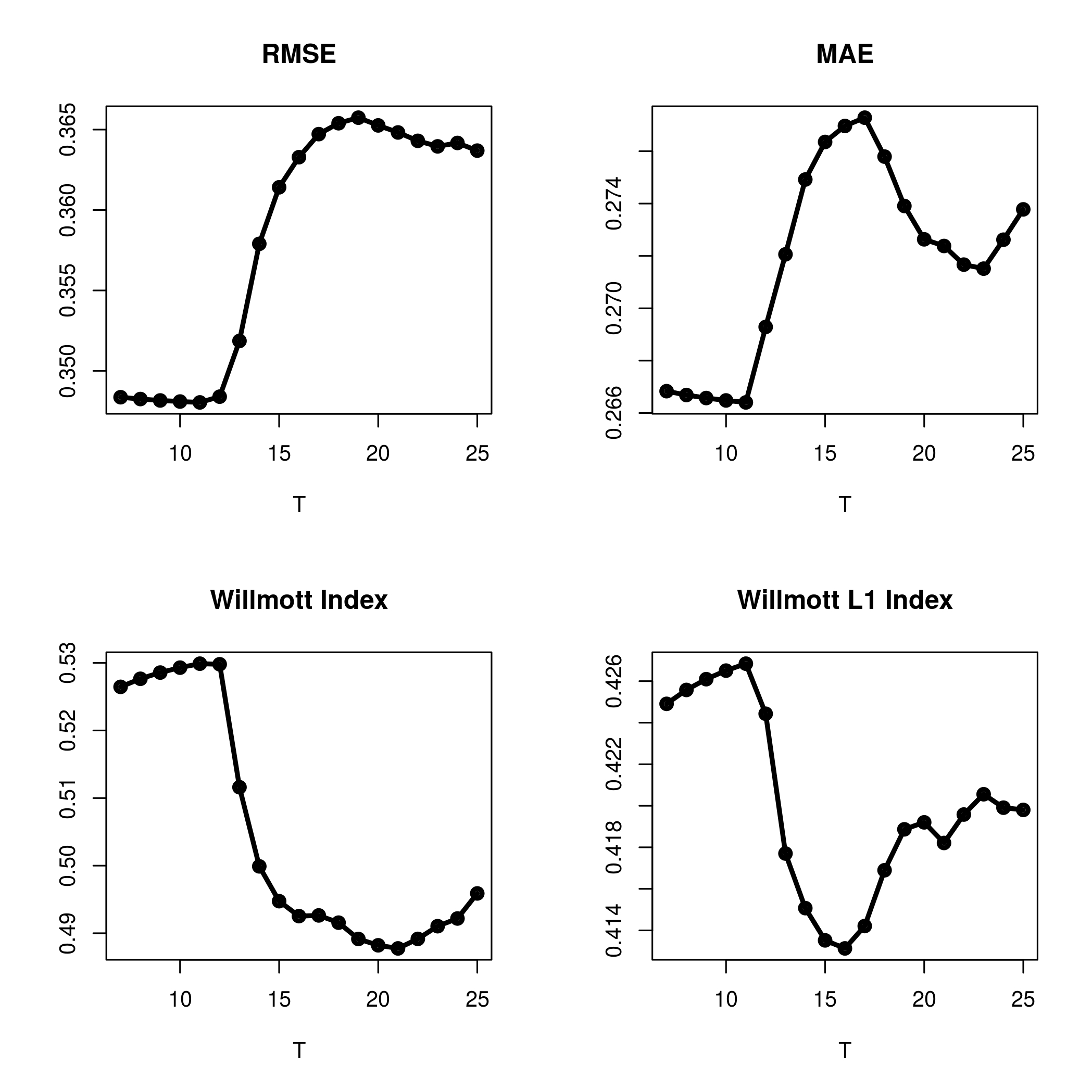
The Series A is a record of $197$ chemical process concentration readings, taken every two hours. This series was introduced by [3], who suggest using an ARMA $\left(1,1\right)$ process to model this data set. An AR $\left(7\right)$ is proposed in [7] and [16]. In Figure 3 we observe that the auto-covariance function of the AR $(7)$ and ARMA $(1,1)$ adjusted models goes to zero very quickly and their auto-covariance structure does not resemble that observed. To obtain a suitable value of $T$ , we calculate the RMSE, MAE and the two indices of Wilmott for values of $T$ between $5$ and $25$ . In each case, we estimate the parameters and calculate the four measures of the quality of prediction for $m=50$ predictions. In Figure 4 we show the values of the four measures for values of $T$ between $7$ and $25$ when we adjusted an FOU $(\lambda^{(2)},\sigma,H)$ model (the values of $T=5$ and $T=6$ had very bad performance and are not included in the figure). Observe that in the four cases, the optimal value is reached for $T=11$ . Also, we can use a neigbourhood of $T=11$ and we have similar performance. In the rest of the adjusted FOU cases, the optimal value was reached in a neighbourhood at $T=12$ or $T=7$ depending on which measure was optimized. In Table 9 we show the values of $W_{2}$ , $RMSE$ , $W_{1}$ and $MAE$ for AR $(7)$ , ARMA $(1,1)$ and different FOU $(p)$ for $p=2,3,4$ . In all the FOU processes considered, we use $T=12$ . For the estimation of $\lambda$ , we have used the $constrOptim$ function of the $R$ package with the conditions $0.01\leq\lambda_{i}\leq 1.5$ (to optimize on a compact $\Lambda$ ) and $\lambda_{i+1}\geq\lambda_{i}+0.01$ (to ensure that $\lambda_{i}<\lambda_{i+1}$ ) for $i=1,2,3$ . The first results of the estimation are $\hat{H}=0.1367,\hat{\sigma}=0.5464.$ For the $\lambda$ , one estimates $\hat{\lambda}=0.1554$ in FOU $(\lambda^{(2)},\sigma,H)$ , $0.1250$ in FOU $(\lambda^{(3)},\sigma,H)$ , $0.1076$ in FOU $(\lambda^{(4)},\sigma,H)$ , $(0.0328,0.2273)$ in FOU $(\lambda_{1},\lambda_{2},\sigma,H)$ , $(0.0123,0.0241,0.2291)$ in FOU $(\lambda_{1},\lambda_{2},\lambda_{3},\sigma,H)$ and $(0.0267,0.0533,0.1163,0.1766)$ in FOU $(\lambda_{1},\lambda_{2},\lambda_{3},\lambda_{4},\sigma,H)$ .

Table 9: Values of

W_{2}

RMSE

W_{1}

and

MAE

for different models adjusted to Series A.

$\begin{array}[]{|c|cccc|}\hline\cr\text{Model}&W_{2}&RMSE&W_{1}&MAE\\ \hline\cr\text{AR}\left(7\right)&0.6184&\textbf{0.2995}&\textbf{0.4943}&\textbf{0.2167}\\ \text{ARMA}\left(1,1\right)&0.5883&0.3120&0.4620&0.2343\\ \text{FOU}\left(\lambda_{1},\lambda_{2},\sigma,H\right)&0.6263&0.3076&0.4743&0.2372\\ \text{FOU}\left(\lambda_{1},\lambda_{2},\lambda_{3},\sigma,H\right)&0.6260&0.3076&0.4743&0.2371\\ \text{FOU}\left(\lambda_{1},\lambda_{2},\lambda_{3},\lambda_{4},\sigma,H\right)&0.6244&0.3074&0.4733&0.2369\\ \text{FOU}\left(\lambda^{\left(2\right)},\sigma,H\right)&0.6247&0.3086&0.4712&0.2393\\ \text{FOU}\left(\lambda^{\left(3\right)},\sigma,H\right)&\textbf{0.6277}&0.3078&0.4750&0.2373\\ \text{FOU}\left(\lambda^{\left(4\right)},\sigma,H\right)&0.6264&0.3076&0.4742&0.2372\\ \hline\cr\end{array}$

We observe that FOU $(\lambda^{(3)},\sigma,H)$ has the best performance in terms of the $L^{2}$ -Willmott Index, and its RMSE is very close to that of the AR $(7)$ model. For the $L^{1}$ the performance is slightly worse than the AR $(7)$ model.

On the other hand, in Figure 3 we observe that the auto-covariances of the AR $(7)$ and ARMA $(1,1)$ adjusted models, go to zero very quickly and their auto-covariance structure does not resemble that observed. Besides the adjusted FOU $(\lambda^{(3)},\sigma,H)$ and FOU $(\lambda^{(4)},\sigma,H)$ have a better performance.

6.2 Water level of Lake Huron

The water level in feet of Lake Huron for 1875–1972, is a time series of $98$ observations. This is a small size to apply our procedure of estimation, which requires $n,T\rightarrow+\infty$ and $T/n\rightarrow 0$ . Then, we can apply Corollary 1, for different values of $H$ and $\sigma=1$ (assuming that the fractional Brownian motion which drives the FOU process is standard). The results for $H=0.5,0.6,0.7$ and $T=10,20,30$ were similiar. Using the procedure to choose the value of $T$ proposed in subsection 5.1, we have obtained that the best performance was for $T=30$ .

The series has a slight trend, which was removed before adjusting the models. In [4], it is suggested to use an AR $\left(2\right)$ and ARMA $\left(1,1\right)$ for this series. Nor are there significant differences between the observed curve and the predictions curve for the the different models in the last 20 observations (Figure 5).

In Table 10, we show the values of $W_{2}$ , $RMSE$ , $W_{1}$ and $MAE$ , for the adjusted AR $(2)$ , ARMA $(1,1)$ and different FOU $(p)$ for $p=2,3,4$ models adjusted for $T=30$ , $H=0.5$ and $\sigma=1$ .

We see that the performances of all models considered are similar. We see that $\text{FOU}\left(\lambda^{(3)},\sigma,H\right)$ model obtains slightly better results, and is clearly better than the AR $(2)$ and ARMA $(1,1)$ models.

Table 10: Values of

W_{2}

RMSE

W_{1}

and

MAE

for different models, adjusted to the series “level in feet, Lake Huron”, for

m=40

predictions and

T=30

H=0.5

\sigma=1

$\begin{array}[]{|c|cccc|}\hline\cr\text{Model}&W_{2}&RMSE&W_{1}&MAE\\ \hline\cr\text{AR}\left(2\right)&0.8421&0.8961&0.6345&0.7262\\ \text{ARMA}\left(1,1\right)&0.8426&0.8999&0.6322&0.7271\\ \text{FOU}\left(\lambda_{1},\lambda_{2},\sigma,H\right)&0.8850&0.7877&0.6903&0.6361\\ \text{FOU}\left(\lambda_{1},\lambda_{2},\lambda_{3},\sigma,H\right)&0.8862&0.7569&0.6967&\textbf{0.6061}\\ \text{FOU}\left(\lambda_{1},\lambda_{2},\lambda_{3},\lambda_{4},\sigma,H\right)&0.8862&\textbf{0.7568}&0.6966&\textbf{0.6061}\\ \text{FOU}\left(\lambda^{\left(2\right)},\sigma,H\right)&0.8788&0.7834&0.6919&0.6192\\ \text{FOU}\left(\lambda^{\left(3\right)},\sigma,H\right)&\textbf{0.8867}&\textbf{0.7568}&\textbf{0.6973}&0.6062\\ \text{FOU}\left(\lambda^{\left(4\right)},\sigma,H\right)&0.8852&0.7572&0.6939&0.6086\\ \hline\cr\end{array}$

To have an idea of how these values can be changed for different values of the number $m$ of predictions, in Figure 6 we show the results of the Willmott Index ( $W_{2}$ ) and MAE for values of $m$ between $10$ to $40$ .

Figure 6 shows that for both measures of the quality of prediction, the FOU models clearly outperform AR $(2)$ and ARMA $(1,1)$ as the number of predictions ( $m$ ) grows.

6.3 Affluent energy generated by hydroelectric dams in Uruguay

In this case we study a time series very different from the ones previously considered. On the one hand, it is longer than them. On the other hand [12] and [11] show that this time series presents a long memory behaviour. We start with the weekly data set of affluent energy generated by hydroelectric dams in Uruguay between the first week of 1909 and the last week of 2012. The observations present a seasonal component that was removed. In [12] there can be found a more detailed description of this time series together with a comparison, taking into account the predictive power, of an ARFIMA $(p,d,q)$ model with an FOU $(\lambda,\sigma,H)$ model. In our case the time series has a sample size of length $5408$ , and we have adjusted FOU $(p)$ models for $p=2,3,4$ with the first $5148$ terms, and we have predicted the next $260$ weeks (this corresponds to the 2009 to 2012). In each case, we have made a one-step prediction (to predict a future value $X_{t}$ we have estimated the parameters using the information from the time series for all times earlier than $t$ ). In [12], an ARFIMA $(1,d,3)$ is proposed to adjust the observations. The performance of the FOU $(p)$ models at estimating the value of $\sigma$ or using $\sigma=1$ are similar, therefore we prefer to take $\sigma=1$ and we have chosen the value of $T$ as suggested in subsection 5.1. In Table 11 we show the values of $T$ and the estimate of $\lambda$ for each model considered. The estimation of $H$ yielded $\hat{H}=0.7114.$ Although the optimal value of $T$ considered is different for each adjusted FOU $(p)$ model, there are little variations for different values of $T$ .

Table 11: Values of

T

considered and values of

\hat{\lambda}

for different FOU

(p)

adjusted models.

$\begin{array}[]{|c|ccccc|}\hline\cr&\text{FOU}\left(\lambda^{\left(2\right)},H\right)&\text{FOU}\left(\lambda^{\left(3\right)},H\right)&\text{FOU}\left(\lambda^{\left(4\right)},H\right)&\text{FOU}\left(\lambda_{1},\lambda_{2},H\right)&\text{FOU}\left(\lambda_{1},\lambda_{2},\lambda_{3},H\right)\\ \hline\cr$T$&280&230&290&200&300\\ \hat{\lambda}&0.3115&0.3595&0.3617&(0.5668,0.5802)&(0.3062,0.3162,0.3267)\\ \hline\cr\end{array}$

In Table 12 we show a comparison, in terms of for the four measures of quality of prediction of the FOU $(p)$ models and ARFIMA $(1,d,3)$ and we include the ARFIMA $(3,d,1)$ model because it was the model that achieved the best predictions for the latest four years (2009 to 2012) from among the ARFIMA $(p.d.q)$ for values of $p,q\in\{0,1,2,3\}$ .

Table 12: Values of

W_{2}

RMSE

W_{1}

and

MAE

for different models, adjusted to the non–stationary series ‘affluent energy generated by hydroelectric dams’, for the years 2009 to 2012 (

\sigma=1

$\begin{array}[]{|c|cccc|c|cccc|}\hline\cr\text{2009}&W_{2}&RMSE&W_{1}&MAE&2010&W_{2}&RMSE&W_{1}&MAE\\ \hline\cr\text{ARFIMA}(3,d,1)&0.8184&\textbf{0.3622}&0.5857&0.2853&&0.9497&0.5074&0.7943&0.3992\\ \text{ARFIMA}(1,d,3)&0.8137&0.3605&0.5827&0.2838&&0.9497&0.5076&0.7900&0.4077\\ \text{FOU}\left(\lambda_{1},\lambda_{2},H\right)&0.8418&0.3782&0.6499&0.2699&&0.9606&0.4940&0.8353&0.3507\\ \text{FOU}\left(\lambda_{1},\lambda_{2},\lambda_{3},H\right)&0.8422&0.3776&0.6510&0.2691&&0.9611&0.4903&0.8365&0.3474\\ \text{FOU}\left(\lambda^{\left(2\right)},H\right)&0.7385&0.3929&0.5168&0.3089&&0.9470&0.5196&0.7934&0.4009\\ \text{FOU}\left(\lambda^{\left(3\right)},H\right)&0.8423&0.3775&0.6511&0.2690&&\textbf{0.9611 }&\textbf{0.4896 }&\textbf{0.8367}&\textbf{0.3465}\\ \text{FOU}\left(\lambda^{\left(4\right)},H\right)&\textbf{0.8445}&0.3755&\textbf{0.6619}&\textbf{0.2619 }&&0.9610&0.4903&0.8363&0.3476\\ \hline\cr\text{2011}&W_{2}&RMSE&W_{1}&MAE&2012&W_{2}&RMSE&W_{1}&MAE\\ \hline\cr\text{ARFIMA}(3,d,1)&0.9270&\textbf{0.6617}&\textbf{0.7668}&\textbf{0.4841}&&\textbf{0.7406}&\textbf{0.5161}&\textbf{0.5549}&\textbf{0.3980}\\ \text{ARFIMA}(1,d,3)&0.9245&0.6684&0.7609&0.5074&&0.7293&0.5165&0.5479&0.3993\\ \text{FOU}\left(\lambda_{1},\lambda_{2},H\right)&0.9291&0.7276&0.7611&0.5559&&0.7004&0.6153&0.5494&0.4535\\ \text{FOU}\left(\lambda_{1},\lambda_{2},\lambda_{3},H\right)&0.9296&0.7242&0.7624&0.5523&&0.7003&0.6147&0.5499&0.4521\\ \text{FOU}\left(\lambda^{\left(2\right)},H\right)&0.9002&0.7786&0.7047&0.6087&&0.6298&0.5393&0.4623&0.4192\\ \text{FOU}\left(\lambda^{\left(3\right)},H\right)&0.9296&0.7224&0.7626&0.5499&&0.7004&0.6139&0.5498&0.4517\\ \text{FOU}\left(\lambda^{\left(4\right)},H\right)&\textbf{0.9300}&0.7179&0.7636&0.5459&&0.6994&0.6142&0.5490&0.4513\\ \hline\cr\end{array}$

From Table 12 we can deduce that in 2009 and 2010, the FOU $(\lambda^{(4)},H)$ model has the best performance. In addition, in 2011 and 2012, the ARFIMA $(3,d,1)$ has the best performance. In general, in the latest four years, performances of ARFIMA $(3,d,1)$ and FOU $(\lambda^{(4)},H)$ are similar with a slight advantage for FOU $(\lambda^{(4)},H)$ in Willmott’s index and a slight advantage for ARFIMA $(3,d,1)$ in the RMSE and MAE measures. Like the example of Series A, the FOU $(p)$ models obtain better results in Willmott’s index.

7 Remarks

1.

In this paper we has shown that the FOU $(p)$ processes can be used to model a wide range of time series varying from short range dependence to long range dependence.
2.

Another advantage to using an FOU $(p)$ process to model a continuous time data set (instead a discrete time model) is that it has a parameter ( $H$ ) that gives a measure of the irregularity of the trajectories in the process. When the time series is in continuous time, the parameter $H$ can give extra information about how irregular the trajectories are.
3.

We have suggested how to obtain a suitable value of $T$ in order to optimize the criterion that is required by the investigator.
4.

In the three real data sets considered, we observe results as shown in Figure 4, that is, little variation between the measures considered in some range of values of $T$ and an abrupt change in the performance out of this range (for example, from $T=5$ to $T=6$ in Figure 4).
5.

In the cases studied in this paper we have shown that it is possible to avoid the estimation of the parameter $\sigma$ (just taking $\sigma=1$ ). In general, we can estimate $\sigma$ using the method proposed in subsection 3.1.

8 Conclusions

In this paper we have presented a way to model an observed time series by a FOU process. We have shown that the FOU $(p)$ processes can be used to model a wide range of time series varying from short range dependence to long range dependence, with performance similar to the ARMA or ARFIMA models and in several cases outperforming them. From theoretical point of view, we have presented a way to extend the theoretical results for FOU $(p)$ processes for $H<1/2$ . We have presented a method to estimate the $\lambda$ parameters when the process is observed on a discretized and equispaced set in an interval $[0,T]$ and proved, under some conditions on $T$ and the sample size $n$ , that this procedure gives a consistent estimator. By simulations we have corroborated the consistency of all the estimators of the parameters. Lastly we have given a complete description of FOU $(2)$ and FOU $(3)$ processes by an explicit formula for their auto-covariance functions, and showed how these explicit formulas can be obtained for the FOU $(p)$ processes for $p\geq 4$ .

9 Proofs

To prove Theorem 4, we need the following lemmas.

Lemma 1.

Under the conditions of Theorem 4 and fixed $\sigma$ and $H$ , then, given $\varepsilon>0$ there exists a $T_{0}>0$ and a random variable $K_{\varepsilon}$ such that

P\left(\sup_{\lambda\in\Lambda}\left|U_{T}\left(\lambda,\sigma,H\right)-U_{T^{\prime}}\left(\lambda,\sigma,H\right)\right|\leq K_{\varepsilon}\left|T-T^{\prime}\right|\text{ }\right)\geq 1-\varepsilon\ \ \text{ for all }T,T^{\prime}\geq T_{0}.

Remark 12.

Lemma 1 together with the completeness of the space of continuous functions defined on a compact $\Lambda$ , allows deducing the existence of a function $U\left(\lambda,\sigma,H\right)$ such that for any fixed $\sigma$ and $H$ , the $U_{T}\left(.,\sigma,H\right)$ converge uniformly on $\Lambda$ to $U\left(.,\sigma,H\right)$ in probability as $T\rightarrow+\infty.$

Proof of Lemma 1.

I_{T}(x)=\frac{1}{2\pi T}\left(\int_{0}^{T}X_{t}\cos\left(tx\right)dt\right)^{2}+\frac{1}{2\pi T}\left(\int_{0}^{T}X_{t}\sin\left(tx\right)dt\right)^{2}:=I_{T}^{\left(1\right)}(x)+I_{T}^{\left(2\right)}(x).

\frac{\partial I_{T}^{\left(1\right)}(x)}{\partial T}=\frac{2TX_{T}\cos\left(Tx\right)\int_{0}^{T}X_{t}\cos\left(tx\right)dt-\left(\int_{0}^{T}X_{t}\cos\left(tx\right)dt\right)^{2}}{2\pi T^{2}}.

Then,

\left|\frac{\partial I_{T}^{\left(1\right)}(x)}{\partial T}\right|\leq\frac{2\left|X_{T}\right|\left|\int_{0}^{T}X_{t}\cos\left(tx\right)dt\right|}{2\pi T}+\frac{1}{2\pi}\left(\frac{1}{T}\int_{0}^{T}X_{t}\cos\left(tx\right)dt\right)^{2}.

Observe that

\frac{\left|\int_{0}^{T}X_{t}\cos\left(tx\right)dt\right|}{T}\leq\frac{\int_{0}^{T}\left|X_{t}\right|dt}{T}.

On the one hand,

\frac{\int_{0}^{T}\left|X_{t}\right|dt}{T}\overset{a.s.}{\rightarrow}\mathbb{E}\left(\left|X_{0}\right|\right)\text{ as }T\rightarrow+\infty

(19)

by the ergodic theorem. On the other hand, observing that the distribution of $X_{T}$ does not depend on $T,$ and $\frac{\left|\int_{0}^{T}X_{t}\cos\left(tx\right)dt\right|}{T}\leq\frac{\int_{0}^{T}\left|X_{t}\right|dt}{T}$ , we obtain that there exists $T_{0}$ and a random variable $K_{\varepsilon}$ such that $\frac{2\left|X_{T}\right|\left|\int_{0}^{T}X_{t}\cos\left(tx\right)dt\right|}{T}$ is bounded for all $T\geq T_{0}$ (and for all $x$ ). Then for all $T\geq T_{0}$ , such that $P\left(\left|\frac{\partial I_{T}^{\left(1\right)}(x)}{\partial T}\right|\leq K_{\varepsilon}\text{ for all }x\right)\geq 1-\varepsilon$ .

Proceeding analogously with $\frac{\partial I_{T}^{\left(2\right)}(x)}{\partial T}$ , we obtain that given $\varepsilon>0,$ there exists a $T_{0}$ and a random variable $K_{\varepsilon}$ such that

P\left(\left|\frac{\partial I_{T}(x)}{\partial T}\right|\leq K_{\varepsilon}\text{ for all}\ x\right)\geq 1-\varepsilon

(20)

for all $T\geq T_{0}.$ Therefore, if $\left|\frac{\partial I_{T}(x)}{\partial T}\right|\leq K_{\varepsilon}$ for all $x$ , then from the mean value theorem we obtain that

\left|U_{T}\left(\lambda,\sigma,H\right)-U_{T^{\prime}}\left(\lambda,\sigma,H\right)\right|\leq\int_{0}^{+\infty}\frac{\left|I_{T}(x)-I_{T^{\prime}}(x)\right|}{f^{\left(X\right)}\left(x,\lambda\right)}w(x)dx\leq

K_{\varepsilon}\left|T-T^{\prime}\right|\int_{0}^{+\infty}\frac{w(x)}{f^{\left(X\right)}\left(x,\lambda\right)}dx,

for all $T,T^{\prime}\geq T_{0}.$ Thus, using that $\int_{0}^{+\infty}\frac{w(x)}{f^{\left(X\right)}\left(x,\lambda\right)}dx$ is bounded on the compact $\Lambda$ and renaming $K_{\varepsilon}$ , we obtain that

\sup_{\lambda\in\Lambda}\left|U_{T}\left(\lambda,\sigma,H\right)-U_{T^{\prime}}\left(\lambda,\sigma,H\right)\right|\leq K_{\varepsilon}\left|T-T^{\prime}\right|.

∎

Lemma 2.

Under the conditions of Theorem 4, then, given $\varepsilon>0$ there exists a $T_{0}$ and a random variable $K_{\varepsilon}$ such that the probability of

\max\left\{\left|\frac{\partial h_{T}}{\partial x}\left(x,\lambda,\sigma,H\right)\right|,\left|\frac{\partial h_{T}}{\partial\sigma}\left(x,\lambda,\sigma,H\right)\right|,\left|\frac{\partial h_{T}}{\partial H}\left(x,\lambda,\sigma,H\right)\right|\right\}\leq K_{\varepsilon}T^{2}

for all $\left(x,\lambda,\sigma,H\right)\in\left[0,T\right]\times\Lambda\times\left[\sigma_{1},\sigma_{2}\right]\times\left[h_{1},h_{2}\right],$ is greater than or equal to $1-\varepsilon$ .

Proof of Lemma 2.

Firstly, we will prove that there exists a $T_{0}>0$ and a random variables $K_{\varepsilon}^{\prime}$ , $K_{\varepsilon}^{\prime\prime}$ such that

P\left(\left|I_{T}(x)\right|\leq K_{\varepsilon}^{\prime}T\text{ for all }x\right)\geq 1-\varepsilon/2\text{ for all }T\geq T_{0}

(21)

and

P\left(\left|\frac{\partial I_{T}}{\partial x}(x)\right|\leq K_{\varepsilon}^{\prime\prime}T^{2}\text{ for all }x\right)\geq 1-\varepsilon/2\text{ for all }T\geq T_{0}.

(22)

Observe that

I_{T}(x)=\frac{1}{2\pi T}\left|\int_{0}^{T}X_{t}e^{itx}dt\right|=\frac{T}{2\pi}\left|\frac{1}{T}\int_{0}^{T}X_{t}e^{itx}dt\right|^{2}\leq\frac{T}{2\pi}\left(\frac{1}{T}\int_{0}^{T}\left|X_{t}\right|dt\right)^{2}

and applying the ergodic theorem to the process $\{|X_{t}|\}_{t\in\mathbb{R}}$ , we deduce (21).

Using that $t\in[0,T]$ and applying the Cauchy–Schwartz inequality, we obtain that

\left|\frac{\partial I_{T}}{\partial x}(x)\right|=

\frac{1}{\pi T}\left|\int_{0}^{T}X_{t}\cos(tx)dt\int_{0}^{T}tX_{t}\sin(tx)dt+\int_{0}^{T}X_{t}\sin(tx)dt\int_{0}^{T}tX_{t}\cos(tx)dt\right|\leq

\frac{2}{\pi}\left(\int_{0}^{T}|X_{t}|dt\right)^{2}\leq\frac{2T}{\pi}\int_{0}^{T}X_{t}^{2}dt.

(23)

Applying the ergodic theorem to the process $\{X_{t}^{2}\}_{t\in\mathbb{R}}$ , we deduce (22).

Consider $\widetilde{\lambda}\in\Lambda$ such that $\lambda_{i}\leq\widetilde{\lambda}_{i}$ for all $i=1,2,...,q.$ Then

\left|\frac{\partial h_{T}}{\partial\sigma}\left(x,\lambda,\sigma,H\right)\right|=\left|\frac{2}{\sigma}-\frac{2I_{T}(x)2\pi\prod_{i=1}^{q}\left(\lambda_{i}^{2}+x^{2}\right)^{q_{i}}}{\sigma^{3}\Gamma\left(2H+1\right)\sin\left(H\pi\right)x^{2p-1-2H}}\right|\frac{w(x)}{2\pi}\leq

\left(\frac{2}{\sigma_{1}}+\frac{c_{1}I_{T}(x)\prod_{i=1}^{q}\left(\widetilde{\lambda}_{i}^{2}+x^{2}\right)^{q_{i}}}{\sigma_{1}^{3}x^{2p-1-2H}}\right)\frac{w(x)}{2\pi}\ \text{where}\ c_{1}\text{ is a constant}.

(24)

Condition $a\geq 2p$ arranges that (24) has no singularity in $x=0.$ On the other hand, condition $b\geq a+3$ arranges that (24) goes to zero as $x\rightarrow+\infty$ . Therefore, from (21) we have that there exists a $T_{0}>0$ and a random variable $K_{\varepsilon}^{(1)}$ such that the probability of $\left|\frac{\partial h_{T}}{\partial\sigma}\left(x,\lambda,\sigma,H\right)\right|\leq K_{\varepsilon}^{(1)}T$ for all $\left(x,\lambda,\sigma,H\right)\in\left[0,T\right]\times\Lambda\times\left[\sigma_{1},\sigma_{2}\right]\times\left[h_{1},h_{2}\right]$ is greater than or equal to $1-\varepsilon/2$ for all $T\geq T_{0}$ .

\left|\frac{\partial h_{T}}{\partial H}\left(x,\lambda,\sigma,H\right)\right|\leq\left|\frac{2\Gamma^{\prime}\left(2H+1\right)}{\Gamma\left(2H+1\right)}+\frac{\pi\cos\left(H\pi\right)}{\sin\left(H\pi\right)}-2\log x\right|w(x)+

\left|\frac{I_{T}(x)\prod_{i=1}^{q}\left(\lambda_{i}^{2}+x^{2}\right)^{q_{i}}}{\sigma^{2}x^{2p-1-2H}}\frac{2\Gamma^{\prime}\left(2H+1\right)\sin\left(H\pi\right)+\pi\Gamma\left(2H+1\right)\cos\left(H\pi\right)}{\left(\Gamma\left(2H+1\right)\sin\left(H\pi\right)\right)^{2}}\right|w(x)+

\left|\frac{I_{T}(x)\prod_{i=1}^{q}\left(\lambda_{i}^{2}+x^{2}\right)^{q_{i}}}{\sigma^{2}x^{2p-1-2H}}\frac{2\log x}{\Gamma\left(2H+1\right)\sin\left(H\pi\right)}\right|w(x).

Analogously to the previous case we obtain that there exists a random variable $K_{\varepsilon}^{(2)}$ such that the probability of $\left|\frac{\partial h_{T}}{\partial H}\left(x,\lambda,\sigma,H\right)\right|\leq K_{\varepsilon}^{(2)}T$ for all $\left(x,\lambda,\sigma,H\right)\in\left[0,T\right]\times\Lambda\times\left[\sigma_{1},\sigma_{2}\right]\times\left[h_{1},h_{2}\right]$ is greater than or equal to $1-\varepsilon/2$ for all $T\geq T_{0}$ .

We call $h_{T}\left(x,\lambda,\sigma,H\right)=g_{T}\left(x,\lambda,\sigma,H\right)\frac{w(x)}{2\pi}$ where

g_{T}\left(x,\lambda,\sigma,H\right)=\ln\left(\frac{\sigma^{2}\Gamma\left(2H+1\right)\sin\left(H\pi\right)x^{2p-1-2H}}{p_{2p}(x)}\right)+\frac{I_{T}(x)p_{2p}(x)}{\sigma^{2}\Gamma\left(2H+1\right)\sin\left(H\pi\right)x^{2p-1-2H}}

and $p_{2p}(x)=2\pi\prod_{i=1}^{q}\left(\lambda_{i}^{2}+x^{2}\right)^{q_{i}}$ is a polynomial of order $2p.$

Then $\left|\frac{\partial g_{T}}{\partial x}\left(x,\lambda,\sigma,H\right)\frac{w(x)}{2\pi}\right|\leq$

\left|\frac{2p-1-2H}{x}-\frac{p_{2p}^{\prime}(x)}{p_{2p}(x)}\right|\frac{w(x)}{2\pi}+

\left|\frac{\left(\frac{\partial I_{T}(x)}{\partial x}p_{2p}(x)+I_{T}(x)p_{2p}^{\prime}(x)\right)x^{2p-1-2H}-\left(2p-1-2H\right)x^{2p-2-2H}I_{T}(x)p_{2p}(x)}{\sigma^{2}\Gamma\left(2H+1\right)\sin\left(H\pi\right)x^{4p-2-4H}}\right|\frac{w(x)}{2\pi}

Analogously to the case $\frac{\partial g_{T}}{\partial x}\left(x,\lambda,\sigma,H\right)$ , observe that conditions $b\geq a+3,$ $a\geq 2p$ allows to affirm that (in a set of prabability greater than or equal to $1-\varepsilon/2$ ) that there exists a random variables $K_{\varepsilon}^{(3)}$ , $K_{\varepsilon}^{(4)}$ such that $\left|\frac{\partial g_{T}}{\partial x}\left(x,\lambda,\sigma,H\right)\frac{w(x)}{2\pi}\right|\leq K_{\varepsilon}^{(3)}T^{2}.$ and $\left|g_{T}\left(x,\lambda,\sigma,H\right)\frac{w^{\prime}\left(x\right)}{2\pi}\right|\leq K_{\varepsilon}^{(4)}T^{2},$ with probability greater than or equal to $1-\varepsilon/2$ . Therefore, there exists a $T_{0}>0$ and a random variable $K_{\varepsilon}=\max\{K_{\varepsilon}^{(1)},K_{\varepsilon}^{(2)},K_{\varepsilon}^{(3)},K_{\varepsilon}^{(4)}\}$ such that the probability of

\max\left\{\left|\frac{\partial h_{T}}{\partial x}\left(x,\lambda,\sigma,H\right)\right|,\left|\frac{\partial h_{T}}{\partial\sigma}\left(x,\lambda,\sigma,H\right)\right|,\left|\frac{\partial h_{T}}{\partial H}\left(x,\lambda,\sigma,H\right)\right|\right\}\leq K_{\varepsilon}T^{2}

for all $\left(x,\lambda,\sigma,H\right)\in\left[0,T\right]\times\Lambda\times\left[\sigma_{1},\sigma_{2}\right]\times\left[h_{1},h_{2}\right],$ is greater than or equal to $1-\varepsilon$ for all $T\geq T_{0}$ . ∎

Lemma 3.

Under the conditions of Theorem 4, we have

\sup_{0\leq x\leq T_{n}}\left|I_{T_{n}}(x)-I_{T_{n}}^{\left(n\right)}(x)\right|\overset{P}{\rightarrow}0\text{ as }n\rightarrow+\infty.

Proof of Lemma 3.

For a fixed $T>0,$

\left|I_{T}(x)-I_{T}^{\left(n\right)}(x)\right|=\left|\frac{1}{2\pi T}\left|\int_{0}^{T}e^{itx}X_{t}dt\right|^{2}-\text{ }\frac{1}{2\pi T}\left|\frac{T}{n}\sum_{j=1}^{n}e^{\frac{ijTx}{n}}X_{\frac{jT}{n}}\right|^{2}\right|\leq

\frac{1}{2\pi T}\left|\left(\int_{0}^{T}\cos\left(tx\right)X_{t}dt\right)^{2}-\text{ }\left(\frac{T}{n}\sum_{j=1}^{n}\cos\left(\frac{jTx}{n}\right)X_{\frac{jT}{n}}\right)^{2}\right|+

\frac{1}{2\pi T}\left|\left(\int_{0}^{T}\sin\left(tx\right)X_{t}dt\right)^{2}-\text{ }\left(\frac{T}{n}\sum_{j=1}^{n}\sin\left(\frac{jTx}{n}\right)X_{\frac{jT}{n}}\right)^{2}\right|\leq

\frac{1}{2\pi T}\left|\left(\int_{0}^{T}\cos\left(tx\right)X_{t}dt-\text{ }\frac{T}{n}\sum_{j=1}^{n}\cos\left(\frac{jTx}{n}\right)X_{\frac{jT}{n}}\right)\left(\int_{0}^{T}\cos\left(tx\right)X_{t}dt+\text{ }\frac{T}{n}\sum_{j=1}^{n}\cos\left(\frac{jTx}{n}\right)X_{\frac{jT}{n}}\right)\right|+

\frac{1}{2\pi T}\left|\left(\int_{0}^{T}\sin\left(tx\right)X_{t}dt-\text{ }\frac{T}{n}\sum_{j=1}^{n}\sin\left(\frac{jTx}{n}\right)X_{\frac{jT}{n}}\right)\left(\int_{0}^{T}\sin\left(tx\right)X_{t}dt+\text{ }\frac{T}{n}\sum_{j=1}^{n}\sin\left(\frac{jTx}{n}\right)X_{\frac{jT}{n}}\right)\right|=

I_{n,T}+I_{n,T}^{\prime}.

On the one hand,

\left|\int_{0}^{T}\cos\left(tx\right)X_{t}dt+\text{ }\frac{T}{n}\sum_{j=1}^{n}\cos\left(\frac{jTx}{n}\right)X_{\frac{jT}{n}}\right|\leq\int_{0}^{T}\left|X_{t}\right|dt+\text{ }\frac{T}{n}\sum_{j=1}^{n}\left|X_{\frac{jT}{n}}\right|\overset{a.s.}{\rightarrow}2\int_{0}^{T}\left|X_{t}\right|dt.

On the other hand,

\left|\int_{0}^{T}\cos\left(tx\right)X_{t}dt-\text{ }\frac{T}{n}\sum_{j=1}^{n}\cos\left(\frac{jTx}{n}\right)X_{\frac{jT}{n}}\right|=

\left|\sum_{j=1}^{n}\int_{(j-1)T/n}^{jT/n}\left(\cos\left(tx\right)X_{t}-\cos\left(\frac{jTx}{n}\right)X_{\frac{jT}{n}}\right)dt\right|\leq

\sum_{j=1}^{n}\int_{(j-1)T/n}^{jT/n}\left|\left(\cos\left(tx\right)-\cos\left(\frac{jTx}{n}\right)\right)X_{t}\right|dt+\sum_{j=1}^{n}\int_{(j-1)T/n}^{jT/n}\left|\cos\left(\frac{jTx}{n}\right)\left(X_{t}-X_{\frac{jT}{n}}\right)\right|dt.

(25)

If $(j-1)T/n\leq t\leq jT/n$ and $0\leq x\leq T,$ then $\left|\cos\left(tx\right)-\cos\left(jTx/n\right)\right|\leq\left|\left(t-jT/n\right)x\right|\leq xT/n\leq T^{2}/n.$ Thus (25) is less than or equal to

\frac{T^{2}}{n}\int_{0}^{T}\left|X_{t}\right|dt+\sum_{j=1}^{n}\int_{(j-1)T/n}^{jT/n}\left|X_{t}-X_{\frac{jT}{n}}\right|dt.

(26)

Condition $T_{n}^{3}/n\rightarrow 0$ (see Remark 7) and replacing $T$ by $T_{n}$ allows to affirm that the first term in (26) goes to zero in probability as $n\rightarrow+\infty.$ To prove that the second term goes to zero too it is enough to prove that $\sum_{j=1}^{n}\int_{(j-1)T/n}^{jT/n}\mathbb{E}\left(\left|X_{t}-X_{\frac{jT}{n}}\right|\right)dt\rightarrow 0$ as $n\rightarrow+\infty.$

\sum_{j=1}^{n}\int_{(j-1)T/n}^{jT/n}\mathbb{E}\left(\left|X_{t}-X_{\frac{jT}{n}}\right|\right)dt\leq\sum_{j=1}^{n}\int_{(j-1)T/n}^{jT/n}\sqrt{\mathbb{E}\left(\left(X_{t}-X_{\frac{jT}{n}}\right)^{2}\right)}dt.

(27)

Using that the variogram of any FOU $\left(p\right)$ process satisfies the equality $v(t)=\mathbb{E}\left(\left(X_{t}-X_{0}\right)^{2}\right)=\frac{\sigma^{2}}{2}\left|t\right|^{2H}+o\left(\left|t\right|^{2H}\right)$ were $t\rightarrow 0$ (Theorem 3.2 of Kalemkerian & León), then there exists a constant $k$ such that $v(t)\leq k|t|^{2H}$ for all $|t|\leq 1.$ Therefore, $\mathbb{E}\left(\left(X_{t}-X_{\frac{jT}{n}}\right)^{2}\right)=v\left(t-jT/n\right)\leq k\left|t-jT/n\right|^{2H}$ and we obtain that (27) is less than or equal to

\sqrt{k}\sum_{j=1}^{n}\int_{(j-1)T/n}^{jT/n}\left(-t+jT/n\right)^{H}dt=\frac{\sqrt{k}T^{H+1}}{\left(H+1\right)n^{H}}.

Condition $\frac{T_{n}^{H+1}}{n^{H}}\rightarrow 0$ (see Remark 7) and replacing $T$ by $T_{n}$ , allows to affirm that $I_{n,T_{n}}\overset{P}{\rightarrow}0.$ Analogously $I_{n,T_{n}}^{\prime}\overset{P}{\rightarrow}0$ . ∎

Lemma 4.

Under the conditions of Theorem 4, we have

\sup_{\lambda\in\Lambda}\left|U_{T_{n}}^{\left(n\right)}\left(\lambda,\widehat{\sigma},\widehat{H}\right)-U_{T_{n}}\left(\lambda,\sigma^{0},H^{0}\right)\right|\overset{P}{\rightarrow}0\ \text{as}\ n\rightarrow+\infty.

Proof of Lemma 4.

Firstly we will prove that for each $T>0$ there exists a random variable $M_{T}$ such that

\sup_{\lambda\in\Lambda}\left|U_{T}^{\left(n\right)}\left(\lambda,\widehat{\sigma},\widehat{H}\right)-U_{T}\left(\lambda,\sigma^{0},H^{0}\right)\right|\leq TM_{T}\left(\frac{T}{2n}+\left|\widehat{\sigma}-\sigma^{0}\right|+\left|\widehat{H}-H^{0}\right|\right)+A_{n,T}

where $A_{n,T_{n}}\overset{P}{\rightarrow}0$ as $n\rightarrow+\infty.$

\left|U_{T}^{\left(n\right)}\left(\lambda,\widehat{\sigma},\widehat{H}\right)-U_{T}\left(\lambda,\sigma^{0},H^{0}\right)\right|=

\left|\sum_{j=1}^{n}\int_{(j-1)T/n}^{jT/n}\left(h_{T}\left(x,\lambda,\sigma^{0},H^{0}\right)-h_{T}^{\left(n\right)}\left(jT/n,\lambda,\widehat{\sigma},\widehat{H}\right)\right)dx\right|\leq

\sum_{j=1}^{n}\int_{(j-1)T/n}^{jT/n}\left|h_{T}\left(jT/n,\lambda,\widehat{\sigma},\widehat{H}\right)-h_{T}^{\left(n\right)}\left(jT/n,\lambda,\widehat{\sigma},\widehat{H}\right)\right|dx+

\sum_{j=1}^{n}\int_{(j-1)T/n}^{jT/n}\left|h_{T}\left(x,\lambda,\sigma^{0},H^{0}\right)-h_{T}\left(jT/n,\lambda,\widehat{\sigma},\widehat{H}\right)\right|dx=A_{n,T}\left(\lambda\right)+B_{n,T}\left(\lambda\right).

Observe that $h_{T}$ has bounded partial derivatives on $\left[0,T\right]\times\Lambda\times\left[a,b\right]\times\left[h_{1},h_{2}\right]$ and using the mean value theorem, there exists a random variable $M_{T}$ such that for any $\lambda\in\Lambda$

B_{n,T}\left(\lambda\right)\leq M_{T}\sum_{j=1}^{n}\int_{(j-1)T/n}^{jT/n}\left[jT/n-x+\left|\widehat{\sigma}-\sigma^{0}\right|+\left|\widehat{H}-H^{0}\right|\right]dx=

M_{T}\left(\frac{T^{2}}{2n}+T\left|\widehat{\sigma}-\sigma^{0}\right|+T\left|\widehat{H}-H^{0}\right|\right).

From Lemma 2, we have $M_{T}\leq K_{T}T^{2}$ , and from condition $\frac{T_{n}^{4}}{n}\rightarrow 0$ (see Remark 7) and replacing $T$ by $T_{n}$ allows to affirm that $\sup_{\lambda\in\Lambda}B_{n,T_{n}}(\lambda)\overset{P}{\rightarrow}0.$

Now, if we define $A_{n,T}=\sup_{\lambda\in\Lambda}A_{n,T}\left(\lambda\right),$ we will prove that $A_{n,T_{n}}\overset{P}{\rightarrow}0.$

We call $M_{n,T}=\sup_{0\leq x\leq T}\left|I_{T}(x)-I_{T}^{\left(n\right)}(x)\right|$ , then

\left|h_{T}\left(x,\lambda,\sigma,H\right)-h_{T}^{\left(n\right)}\left(x,\lambda,\sigma,H\right)\right|=

\left|I_{T}(x)-I_{T}^{\left(n\right)}(x)\right|\frac{w(x)}{f^{\left(X\right)}\left(x,\lambda,\sigma,H\right)}\leq\frac{M_{n,T}w(x)}{f^{\left(X\right)}\left(x,\lambda,\sigma,H\right)}.

Thus

A_{n,T}\left(\lambda\right)=\frac{T}{n}\sum_{j=1}^{n}\left|h_{T}\left(jT/n,\lambda,\widehat{\sigma},\widehat{H}\right)-h_{T}^{\left(n\right)}\left(jT/n,\lambda,\widehat{\sigma},\widehat{H}\right)\right|dx\leq

M_{n,T}\frac{T}{n}\sum_{j=1}^{n}\frac{w\left(jT/n\right)}{f^{\left(X\right)}\left(jT/n,\lambda,\widehat{\sigma},\widehat{H}\right)}.

Observe that there exists $\widetilde{\lambda}\in\Lambda$ such that $\prod_{i=1}^{q}\left(\lambda_{i}^{2}+x^{2}\right)^{p_{i}}\leq\prod_{i=1}^{q}\left(\widetilde{\lambda}_{i}^{2}+x^{2}\right)^{p_{i}},$ and there exists a constant $k$ such that

\frac{1}{f^{\left(X\right)}\left(x,\lambda,\sigma,H\right)}=\frac{2\pi\prod_{i=1}^{q}\left(\lambda_{i}^{2}+x^{2}\right)^{p_{i}}x^{2H-1-2p}}{\sigma^{2}\Gamma\left(2H+1\right)\sin\left(H\pi\right)}\leq k\prod_{i=1}^{q}\left(\widetilde{\lambda}_{i}^{2}+x^{2}\right)^{p_{i}}x^{2H-1-2p}.

(28)

Using that $H\in\left[h_{1},h_{2}\right]$ there exists $h^{\prime}\in[h_{1},h_{2}]$ such that (28) is less than or equal to

k\prod_{i=1}^{q}\left(\widetilde{\lambda}_{i}^{2}+x^{2}\right)^{p_{i}}x^{2h^{\prime}-1-2p}:=g(x).

Therefore

A_{n,T}\left(\lambda\right)\leq M_{n,T}\frac{T}{n}\sum_{j=1}^{n}\frac{w\left(jT/n\right)}{f^{\left(X\right)}\left(jT/n,\lambda,\widehat{\sigma},\widehat{H}\right)}\leq M_{n,T}\frac{T}{n}\sum_{j=1}^{n}w\left(jT/n\right)g\left(jT/n\right).

Observe that $\frac{T_{n}}{n}\sum_{j=1}^{n}w\left(jT_{n}/n\right)g\left(jT_{n}/n\right)\overset{a.s.}{\rightarrow}\int_{0}^{+\infty}w(x)g(x)dx<+\infty$ and using Lemma 3, we have $M_{n,T_{n}}\overset{P}{\rightarrow}0$ we obtain that $A_{n,T_{n}}=\sup_{\lambda\in\Lambda}A_{n,T_{n}}\left(\lambda\right)\overset{P}{\rightarrow}0.$ ∎

Proof of Theorem 4.

Fix $T>0.$ Given $\varepsilon>0,$ because the minimum of $U_{T}\left(\lambda,\sigma^{0},H^{0}\right)$ is reached in a unique point $\widehat{\lambda}_{T},$ we deduce that there exists a random variable $\delta_{T}>0$ such that the condition $U_{T}\left(\lambda,\sigma^{0},H^{0}\right)<U_{T}\left(\widehat{\lambda}_{T},\sigma^{0},H^{0}\right)+\delta_{T}$ implies that $\left|\widehat{\lambda}_{T}-\lambda\right|<\varepsilon.$ Theorem 3.6 of Kalemkerian & León ([13]) shows that $\widehat{\lambda}_{T}\overset{P}{\rightarrow}\lambda^{0}$ as $T\rightarrow+\infty,$ then $\widehat{\lambda}_{T_{n}}\overset{P}{\rightarrow}\lambda^{0}$ as $n\rightarrow+\infty.$ Also $\widehat{\lambda}_{T}$ is reached in a unique point, then given $\varepsilon,\varepsilon^{\prime}>0$ there exists $T_{0}>0$ and a random variable $\delta_{T_{0}}>0$ such that $P\left(\left|\widehat{\lambda}_{T}-\lambda^{0}\right|\leq\varepsilon/2\right)\geq 1-\varepsilon^{\prime}/2$ for all $T\geq T_{0}$ and

\left\{U_{T_{0}}\left(\lambda,\sigma^{0},H^{0}\right)<U_{T_{0}}\left(\widehat{\lambda}_{T_{0}},\sigma^{0},H^{0}\right)+\delta_{T_{0}}\right\}\subset\left\{\left|\lambda-\widehat{\lambda}_{T_{0}}\right|\leq\varepsilon/2\right\}.

(29)

Also, $\widehat{\lambda}_{T_{n}}\overset{P}{\rightarrow}\lambda^{0}$ it follows that exist $n_{0}$ such that for any $n\geq n_{0}$ the following conditions are fulfilled:

P\left(A_{n}\right)=P\left(\left|\widehat{\lambda}_{T_{n}}-\lambda^{0}\right|\leq\varepsilon/2\right)\geq 1-\varepsilon^{\prime}/4,\text{ }

(30)

P\left(B_{n}\right)=P\left(\left|U_{T_{0}}\left(\widehat{\lambda}_{T_{0}},\sigma^{0},H^{0}\right)-U_{T_{0}}\left(\widehat{\lambda}_{T_{n}},\sigma^{0},H^{0}\right)\right|\leq\delta_{T_{0}}/5\right)\geq 1-\varepsilon^{\prime}/4,

(31)

P\left(C_{n}\right)=P\left(\sup_{\lambda\in\Lambda}\left|U_{T_{0}}\left(\lambda,\sigma^{0},H^{0}\right)-U_{T_{n}}\left(\lambda,\sigma^{0},H^{0}\right)\right|\leq\delta_{T_{0}}/5\right)\geq 1-\varepsilon^{\prime}/4,

(32)

P\left(D_{n}\right)=P\left(\sup_{\lambda\in\Lambda}\left|U_{T_{n}}^{\left(n\right)}\left(\lambda,\widehat{\sigma},\widehat{H}\right)-U_{T_{n}}\left(\lambda,\sigma^{0},H^{0}\right)\right|\leq\delta_{T_{0}}/5\right)\geq 1-\varepsilon^{\prime}/4.\text{ \ }

(33)

(31) it follows from continuity of $U_{T_{0}}$ , (32) from Lemma 1 and (33) from Lemma 4.
Suppose that $A_{n}\cap B_{n}\cap C_{n}\cap D_{n}$ occurs.

On the one hand, from (33) and (13), the definition of $\widehat{\lambda}_{T_{n}}^{(n)}$ , we obtain that

U_{T_{n}}\left(\widehat{\lambda}_{T_{n}}^{\left(n\right)},\sigma^{0},H^{0}\right)\leq U_{T_{n}}^{\left(n\right)}\left(\widehat{\lambda}_{T_{n}}^{\left(n\right)},\widehat{\sigma},\widehat{H}\right)+\delta_{T_{0}}/5\leq

U_{T_{n}}^{\left(n\right)}\left(\widehat{\lambda}_{T_{n}},\widehat{\sigma},\widehat{H}\right)+\delta_{T_{0}}/5\leq U_{T_{n}}\left(\widehat{\lambda}_{T_{n}},\sigma^{0},H^{0}\right)+2\delta_{T_{0}}/5.

Then

U_{T_{n}}\left(\widehat{\lambda}_{T_{n}}^{\left(n\right)},\sigma^{0},H^{0}\right)\leq U_{T_{n}}\left(\widehat{\lambda}_{T_{n}},\sigma^{0},H^{0}\right)+2\delta_{T_{0}}/5.

(34)

On the other hand, from (32) and (34) it follows that

U_{T_{0}}\left(\widehat{\lambda}_{T_{n}}^{\left(n\right)},\sigma^{0},H^{0}\right)\leq U_{T_{n}}\left(\widehat{\lambda}_{T_{n}}^{\left(n\right)},\sigma^{0},H^{0}\right)+\delta_{T_{0}}/5\leq U_{T_{n}}\left(\widehat{\lambda}_{T_{n}},\sigma^{0},H^{0}\right)+3\delta_{T_{0}}/5.

(35)

Also, (32) and (31) implies that

U_{T_{n}}\left(\widehat{\lambda}_{T_{n}},\sigma^{0},H^{0}\right)\leq U_{T_{0}}\left(\widehat{\lambda}_{T_{n}},\sigma^{0},H^{0}\right)+\delta_{T_{0}}/5\leq

(36)

U_{T_{0}}\left(\widehat{\lambda}_{T_{0}},\sigma^{0},H^{0}\right)+2\delta_{T_{0}}/5.

(37)

From (35), (36) and (37) we obtain

U_{T_{0}}\left(\widehat{\lambda}_{T_{n}}^{\left(n\right)},\sigma^{0},H^{0}\right)\leq U_{T_{0}}\left(\widehat{\lambda}_{T_{0}},\sigma^{0},H^{0}\right)+\delta_{T_{0}}

and from (29), we obtain $\left|\widehat{\lambda}_{T_{n}}^{\left(n\right)}-\widehat{\lambda}_{T_{0}}\right|$ $\leq\varepsilon/2,$ thus $\left|\widehat{\lambda}_{T_{n}}^{\left(n\right)}-\lambda^{0}\right|$ $\leq\varepsilon.$

Then, we have shown that $A_{n}\cap B_{n}\cap C_{n}\cap D_{n}\subset\left\{\left|\widehat{\lambda}_{T_{n}}^{\left(n\right)}-\lambda^{0}\right|\leq\varepsilon\right\}$ , therefore $P\left(\left|\widehat{\lambda}_{T_{n}}^{\left(n\right)}-\lambda^{0}\right|\leq\varepsilon\right)\geq 1-\varepsilon^{\prime}$ for all $n\geq n_{0}.$

∎

Proof of Proposition 1.

Formula (14) is given in [13].
(15) it is immediately by taking limit $\beta\rightarrow 0$ in (17).

∎

Proof of Proposition 2.

The formula (16) is given in [13].
To obtain (17), it is enough to take $\lim_{\gamma\rightarrow\alpha}$ in (16). Firstly, to simplify the calculation, we put $a=\alpha^{2},$ $b=\beta^{2}$ and $c=\gamma^{2}.$ Then (16) becomes

\mathbb{E}\left(X_{0}X_{t}\right)=\frac{\sigma^{2}H}{2}\left[\frac{a^{2-H}f_{H}\left(\sqrt{a}t\right)}{\left(a-b\right)\left(a-c\right)}+\frac{b^{2-H}f_{H}\left(\sqrt{b}t\right)}{\left(b-a\right)\left(b-c\right)}+\frac{c^{2-H}f_{H}\left(\sqrt{c}t\right)}{\left(c-a\right)\left(c-b\right)}\right].

(38)

Thus, when $c\rightarrow a$ (38) this becomes

\frac{\sigma^{2}H}{2}\left[\frac{b^{2-H}f_{H}\left(\sqrt{b}t\right)}{\left(b-a\right)^{2}}+\lim_{c\rightarrow a}\frac{a^{2-H}f_{H}\left(\sqrt{a}t\right)\left(c-b\right)-c^{2-H}f_{H}\left(\sqrt{c}t\right)\left(a-b\right)}{\left(a-b\right)\left(a-c\right)\left(c-b\right)}\right]=

\frac{\sigma^{2}H}{2}\left[\frac{b^{2-H}f_{H}\left(\sqrt{b}t\right)}{\left(b-a\right)^{2}}+\frac{1}{\left(b-a\right)^{2}}\lim_{c\rightarrow a}\frac{a^{2-H}f_{H}\left(\sqrt{a}t\right)\left(c-b\right)-c^{2-H}f_{H}\left(\sqrt{c}t\right)\left(a-b\right)}{a-c}\right].

(39)

Applying L’Hôpital rule we obtain that (39) is equal to $\frac{\sigma^{2}H}{2\left(b-a\right)^{2}}\times$

b^{2-H}f_{H}\left(\sqrt{b}t\right)-\lim_{c\rightarrow a}\left[a^{2-H}f_{H}\left(\sqrt{a}t\right)-\left(\left(2-H\right)c^{1-H}f_{H}\left(\sqrt{c}t\right)+\frac{c^{3/2-H}t}{2}f_{H}^{\prime}\left(\sqrt{c}t\right)\right)\left(a-b\right)\right]=

\frac{\sigma^{2}H}{2}\left[\frac{b^{2-H}f_{H}\left(\sqrt{b}t\right)-a^{2-H}f_{H}\left(\sqrt{a}t\right)+\left(\left(2-H\right)a^{1-H}f_{H}\left(\sqrt{a}t\right)+\frac{a^{3/2-H}t}{2}f_{H}^{\prime}\left(\sqrt{a}t\right)\right)\left(a-b\right)}{\left(b-a\right)^{2}}\right].

(40)

Lastly, replacing $a=\alpha^{2}$ and $b=\beta^{2}$ , we obtain (17).

This concludes the proof of (17).

To prove (18) as was done in the previous formula, it is enough to take limit where $b\rightarrow a$ in (40). Then applying L’Hôpital’s rule we obtain that

\frac{\sigma^{2}H}{2}\left[\lim_{b\rightarrow a}\frac{b^{2-H}f_{H}\left(\sqrt{b}t\right)-a^{2-H}f_{H}\left(\sqrt{a}t\right)+\left(\left(2-H\right)a^{1-H}f_{H}\left(\sqrt{a}t\right)+\frac{a^{3/2-H}t}{2}f_{H}^{\prime}\left(\sqrt{a}t\right)\right)\left(a-b\right)}{\left(b-a\right)^{2}}\right]=

\frac{\sigma^{2}H}{4}\left[\lim_{b\rightarrow a}\frac{\left(2-H\right)b^{1-H}f_{H}\left(\sqrt{b}t\right)+\frac{b^{3/2-H}t}{2}f_{H}\left(\sqrt{b}t\right)-\left(2-H\right)a^{1-H}f_{H}\left(\sqrt{a}t\right)-\frac{a^{3/2-H}t}{2}f_{H}^{\prime}\left(\sqrt{a}t\right)}{b-a}\right].

(41)

Applying again L’Hôpital’s rule, (41) is equal to

\frac{\sigma^{2}H}{4}\left[\left(2-H\right)\left(1-H\right)a^{-H}f_{H}\left(\sqrt{a}t\right)+\left(7-4H\right)\frac{a^{1/2-H}t}{2}f_{H}^{\prime}\left(\sqrt{a}t\right)+\frac{a^{1-H}t^{2}}{4}f_{H}^{\prime\prime}\left(\sqrt{a}t\right)\right].

Lastly, putting $a=\alpha^{2}$ we obtain (18). ∎

References

[1] Arratia, A., Cabaña, A. & Cabaña, E., A construction of Continuous time ARMA models by iterations of Ornstein-Uhlenbeck process, SORT Vol 40 (2) 267-302, (2016).
[2] Bardet., J. M. and Bertrand R., A non parametric estimation of the espectral density of a continuous-time Gaussian process observed at random times. times. hal-00276735v3, (2008).
[3] Box, G. E. P., Jenkins, G. M. & Reinsel, G. C., Time Series Analysis, Forecasting and Control, Prentice Hall, (1994).
[4] Brockwell, P. J., Davies, R. A., Introduction to Time Series and Forecasting, Springer, (2002).
[5] Brouste, A. & Iacus, S. M., Parameter estimation for the discretely observed fractional Ornstein-Uhlenbeck process and the Yuima R package, Comput Stat 28: 1529-1547 (2013).
[6] Cheridito, P., Kawaguchi, H. & Maejima, M., Fractional Ornstein-Uhlenbeck Processes. Electronic Journal of Probability, 8(3): 1-14, (2003).
[7] Cleveland, W. S., “The inverse autocorrelations of a time series and their applicattions”. Technometrics, 14: 277-298, (1971).
[8] Ibragimov, I. A. & Rozanov, Y. A., Gaussian random processes. Springer Verlag, (1978).
[9] Istas, I. & Lang, G., Quadratic variations and estimation of the local Hölder index of a Gaussian process. Annals de l’Institute Henry Poincaré, 23(4): 407-436, (1997).
[10] Kalemkerian, J., A truncated Cramér–von Mises test of normality. Communications in Statistics - Theory and Methods, 48:16, 3956-3975 (2019).
[11] Kalemkerian, J., Performance de distintos modelos Farima ajustados a la serie de aportes hidrológicos a las represas de Uruguay. Actas del X Clatse, Córdoba, (2012).
[12] Kalemkerian, J., Prediction using ARFIMA and FOU models of affluent energy. Memoria Investigaciones en Ingeniería, 15, 109-124, (2017).
[13] Kalemkerian, J. & León, J. R, Fractional iterated Ornstein-Uhlenbeck Processes. ALEA, 16, 1105-1124, (2019).
[14] N.N. Leonenko, L.M. Sakhno On the Whittle estimators for some classes of continuous-parameter random processes and fields. Stat. And Prob. Lett. 76, 781-795 (2006).
[15] Lii, K. S. and Masry, E., Fitting for Continuous-Time Stationary Processes from Discrete-Time Data. Journal of Multivariate Analysis 41 56-79, (1992).
[16] McLeod, A. I. & Zang, Y., “Partial autocorrelation parametrization for subset autoregression”. Journal of Time Series Analysis, 27: 599-612, 2006.
[17] Pipiras, V. and Taqqu, M., Integration questions related to fractional Brownian motion, Prob. Th. Rel. Fields, 118, 121-291, (2000).
[18] Willmott, C. J., Some comments of the evaluation of model performance. Buletin of the American Meteorological Society, 63, 1309-1313, 1982.
[19] Xiao, W., Zhang, W. & Xu, D. ”Parameter estimation for fractional Ornstein–Uhlenbeck process at discrete observation”. Applied Mathematical Modelling 35, 4196-4207 (2011).

Modelling and Parameter Estimation for Discretely Observed Fractional Iterated Ornstein–Uhlenbeck Processes

Abstract

1 Introduction

2 Definitions and properties

Definition 1.

Definition 2.

Remark 1.

Remark 2.

Notation 1.

Remark 3.

Remark 4.

Remark 5.

3 Parameter estimation

3.1 Estimation of HH and σ\sigma

Definition 3.

Definition 4.

Theorem 2 (Kalemkerian & León).

Remark 6.

3.2 Estimation of the λ\lambda parameters

Theorem 3 (Kalemkerian & León).

Theorem 4.

Remark 7.

Remark 8.

Corollary 1.

Remark 9.

Remark 10.

Proposition 1.

Proposition 2.

Remark 11.

4 A simulation study

4.1 Consistency of the estimators

4.2 Asymptotic distribution of the estimators

5 Modelling an observed time series using FOU(p)(p) processes

5.1 Choosing the value of TT

6 Applications to real data

6.1 Box, Jenkins and Reinsel “Series A”

6.2 Water level of Lake Huron

6.3 Affluent energy generated by hydroelectric dams in Uruguay

7 Remarks

8 Conclusions

9 Proofs

Lemma 1.

Remark 12.

Proof of Lemma 1.

Lemma 2.

Proof of Lemma 2.

Lemma 3.

Proof of Lemma 3.

Lemma 4.

Proof of Lemma 4.

Proof of Theorem 4.

Proof of Proposition 1.

Proof of Proposition 2.

References

3.1 Estimation of $H$ and $\sigma$

3.2 Estimation of the $\lambda$ parameters

5 Modelling an observed time series using FOU $(p)$ processes

5.1 Choosing the value of $T$