Dust Reverberation of 3C 273: torus structure and lag - luminosity relationJournal: ApJ
Abstract
We monitored the 0.158 quasar 3C 273 between 2015 and 2019 in the optical () and near-infrared (NIR, ) with the aim to perform dust reverberation mapping. Accounting for host galaxy and accretion disk contributions, we obtained pure dust light curves in . Cross correlations between the -band and the dust light curves yield an average rest-frame delay for the hot dust of 410 days. This is a factor 2 shorter than expected from the the dust ring radius 900 light days reported from interferometric studies. The dust covering factor (CF) is about 8%, much smaller than predicted from the half covering angle of found for active galactic nuclei (AGN). We analyse the asymmetric shape of the correlation functions and explore whether an inclined bi-conical bowl-shaped dust torus geometry could bring these findings (, and CF) into a consistent picture. The hot varying dust emission originates from the edge of the bowl rim with a small covering angle , and we see only the near side of the bi-conus. Such a dust gloriole with ld and an inclination matches the data remarkably well. Comparing the results of 3C 273 with literature for less luminous AGN, we find a lag–luminosity relation with , flatter than the widely adopted relation with 0.5. We address several explanations for the new lag–luminosity relation.
Keywords:
Active galactic nuclei (16), Reverberation mapping (2019), Quasars (1319), Photometry (1234)I Introduction
The quasar paradigm comprises a supermassive black hole (SMBH), a central X-ray source, an accretion disk (AD), surrounded by a broad line region (BLR), and a molecular dusty torus (TOR) farther out. The three components AD, BLR and TOR may have smooth transitions between each other rather than being separated entities with sharp boundaries. Of particular interest here is the 3-dimensional geometry of the central region and the three components.
As the inner quasar regions cannot be resolved by conventional imaging techniques, reverberation mapping (RM) is the main tool of the trade (Bahcall et al. 1972; Cherepashchuk & Lyutyi 1973; Gaskell & Sparke 1986; Peterson 1993; Horne et al. 2004). RM traces the delayed response of irradiated regions to the light fluctuations of the continuum emission from the inner AD. As a first approximation, the size of the irradiated region can be inferred from the time lag . This way, near-infrared (NIR) RM studies of the dusty torus find a radius (Clavel et al. 1989; Suganuma et al. 2006).
I.1 The size - luminosity relation
A remarkable finding is the relation between the reverberation based size, , and the AGN luminosity, , with and (Suganuma et al. 2006; Gaskell et al. 2007; Koshida et al. 2014; Minezaki et al. 2019). Such a relation with has been expected, if the hot NIR emitting dust is located in a simple equatorial geometry and measures the dust sublimation radius, , inferred from the UV luminosity (Barvainis 1987). This relation may hold the key for cosmological applications to measure quasar distances and to check for dark energy (Kobayashi et al. 1998; Oknyanskij 1999; Yoshii 2002; Yoshii et al. 2014; Hönig 2014). However, is about 3 times smaller than (Kishimoto et al. 2007; Koshida et al. 2014). This suggests that internal effects like from the 3-dimensional dust geometry or from a reduced heating of potentially shielded dust clouds (Gaskell et al. 2007) need to be better understood, before cosmological implications from the relation should be drawn.
Before we address such effects, we note that a similar relation had been found between the size of the broad line region (BLR) and the AGN luminosity: in the first observational estimate of the R-L relationship Koratkar & Gaskell 1991a found a slope for C IV. Subsequently, for Kaspi et al. 2000 report and then Bentz et al. 2013 after correction of the host galaxy contribution refined this slope to . One more piece to the puzzle was added by Du et al. 2016 reporting for AGN with high accretion rates a shallow slope . Possible explanations for that have been considered, involving the ionisation parameter (Czerny et al. 2019). Notably, nearly half a century ago Dibai 1977 used the Strömgren-type argument and a value of for calculating the first single-epoch AGN black hole masses, which agree remarkably well with the latest reverberation based estimates (Bochkarev & Gaskell 2009).
I.2 The torus structure
Interferometric band measurements with the KECK interferometer (Kishimoto et al. 2009; Kishimoto et al. 2011) and the VLTI/Gravity instrument (GRAVITY Collaboration et al. 2019) resolved the innermost dusty structure of 15 AGN (8 with KECK, 8 with VLTI, and 3C 273 in common). The effective ring radii derived from the observed visibilities scale roughly with the AGN luminosity , but the GRAVITY Collaboration et al. 2019 report a relative size decline in the two highest luminosity AGN. For AGN with available band reverberation measurements, is, on average, larger than . Kishimoto et al. 2011 suggested that the interferometric measurements at least partly resolve the dust sublimation zone, and that the ratio yields information on the compactness () or extent () of the hot dust distribution. For the entire sample, however, is systematically smaller than . To match with , Kishimoto et al. 2007; Kishimoto et al. 2009 suggested that the dust grain sizes are larger or that the central engine radiation is significantly anisotropic.
Kawaguchi & Mori 2010; Kawaguchi & Mori 2011 proposed a bowl-shaped dust torus which smoothly continues into the central AD. In their model, the AD emission is anisotropic, being highest toward the polar region and lowest toward the equatorial region. The anisotropy of the AD emission controls the angle-dependent dust sublimation radius and thus the concave rim of the bowl, allowing for parts of the dust to lie closer to the AD than calculated from the luminosity towards the polar direction. Despite attractive features, however, this model needs to be expanded to account for the influence of the BLR onto the entire system (Goad et al. 2012).
For the well studied Seyfert-1 galaxy NGC 5548, Gaskell et al. 2007 have analyzed the AGN energy budget and derived crucial constraints on the geometry of the BLR and the dust torus: the BLR has a likely covering factor about 40%, which translates to a half covering angle , as measured from the equatorial plane. The BLR shields a substantial fraction of the dust torus from direct illumination by the AD, allowing for the observed relatively small (20%) NIR contribution to the AGN energy budget.
Goad et al. 2012 combined the findings by Gaskell et al. 2007 and Kawaguchi & Mori 2010; Kawaguchi & Mori 2011 into a BLR-TOR system confined by a paraboloidal bowl-shaped torus rim where the BLR clouds lie close to and above the rim (their Fig. 1). The observer sees only the emission from the near side of the bi-polar bowl. The BLR clouds shield part of the dust from the AD radiation at , so that the hot dust emission arises essentially from the top rim of the bowl at . Goad et al. 2012 tested their model with reverberation data of NGC 5548.
Based on high-cadence dust RM observations of the Sy-1 WPVS 48, Pozo Nuñez et al. 2014 found an exceptionally sharp NIR echo, which led them to favour that the varying hot dust is essentially located at the edge () rather than along the entire bowl rim which crosses a large range of iso-delay surfaces. In a slightly generalized view Oknyansky et al. 2015 proposed that the hot dust emission comes from the near side of a hollow bi-conical outflow which is co-spatial with the iso-delay paraboloids, a case requiring that the inclination to the line-of-sight is small. Based on observations of the Sy-1 galaxy 3C 120, with a jet inclination , Ramolla et al. 2018 found that the hot dust echo is relatively sharp and symmetric in contrast to the more complex broad H echo. This is consistent with a paraboloidal bowl model where the BLR is spread over many iso-delay surfaces, yielding the smeared and structured H echo as observed, while the hot dusty bowl-edge matches a relatively narrow range of iso-delay contours. The important feature of such a gloriole-like dust emission is the geometric foreshortening effect of the reverberation signal, because the dust lies above the equatorial plane and closer to the observer. While such structure studies have been performed for Seyfert galaxies, i.e. low luminosity AGN, they should be extended to higher luminosity quasars, in order to recognize luminosity-dependent trends.
I.3 3C 273
3C 273 at is the most luminous nearby quasar and may serve as a bench mark for any luminosity-dependent relations. 3C 273 is the brightest quasar making it an ideal target for observations of any kind.
Based on their 7 years long RM campaign Kaspi et al. 2000 determined rest frame Balmer line lags of d, d and d versus the band; here is the centroid of the interpolated cross correlation function. Kishimoto et al. 2011 and GRAVITY Collaboration et al. 2019 reported a dust ring radius of ld inferred from interferometric band measurements.
Yet, to our knowledge, no dedicated dust reverberation mapping campaign of 3C 273 has been performed. Fortunately, Soldi et al. 2008 have collected all published photometry of 3C 273 of the past 50 years in the ISDC11 1 http://isdc.unige.ch/3c273/, Geneva, adjusted the photometry from different telescopes, removed flares, selected the best data. Cross correlating the with optical and UV light curves, they derived a rest frame dust lag of years. An important part of these data are the light curves obtained by Neugebauer & Matthews 1999 at the 5 m Palomar Hale telescope between 1974 and 1998, using a single-element InSb photovoltaic detector and chopping/nodding technique to remove the effects of the sky emission; as described by Soldi et al. these data unfortunately were not available in tabulated form but extracted from the figure.
Remarkably the dust lag (365 d) is shorter than the H lag (443 d), a fact which at first glance suggests the dust torus to be smaller than the BLR, hence appears in contradiction to the AGN unified scheme (Antonucci 1993). This led us to embark on a dedicated reverberation campaign of 3C 273, and we here report on the results of the dust reverberation, a re-analysis of Soldi et al.’s data, a comparison with bowl-shaped models and the interferometric measurements, and the impact on the lag–luminosity relation.
Section II describes the observations and data. Section III shows the light curves, the determination and subtraction of the host galaxy and the contribution of the AD to the NIR light curves, the properties of the varying dust emission, the dust time lag and the derivation of the dust covering factor. Section IV considers the RM results in the framework of a bowl-shaped TOR geometry using the additional constraints of the interferometric size and the small dust covering factor. Section V discusses the findings and implications. Section VI provides a summary and conclusions. Throughout this paper we adopt , and H∘ = 73 km s-1 Mpc-1 yielding an angular-size distance of 546 Mpc (luminosity distance of 734 Mpc) for 3C 273.
II Observations and data reduction
3C 273 was observed between April 2015 and June 2019 with semi-robotic optical and NIR telescopes of the Bochum University Observatory near Cerro Armazones (OCA)in Chile22 2 https://en.wikipedia.org/wiki/Cerro_Armazones_Observatory (Ramolla et al. 2016). The optical telescopes used are: the 40 cm Bochum Monitoring Telescope, BMT (Ramolla et al. 2013); the 15 cm Robotic Bochum Twin Telescope ROBOTT (formerly named VYSOS 6, for short V6) (Haas et al. 2012); the 25 cm BEST-II (Kabath et al. 2009) and the 80 cm infrared telescope IRIS (Hodapp et al. 2010).
Typically dithered images were taken per filter and night and later combined. All images were reduced by the corresponding instrumental data reduction pipelines (dark, bias and flat correction). Astrometric matching was performed with Scamp (Bertin 2006). Before stacking multiple exposures, they were resampled onto a common coordinate grid with pixel size using Swarp (Bertin et al. 2002); the seeing has typically a point spread function of 3 FWHM. The photometry is performed on combined frames with a fixed 75 aperture found to be the optimum in our previous studies, e.g. (Haas et al. 2011; Pozo Nuñez et al. 2014; Ramolla et al. 2018).
| Filter | [m] | [Jy] | avg.Flux [mJy] | Obs.nights |
|---|---|---|---|---|
| 0.433 | 4266.7 | 23.04 1.39 | 109 | |
| 0.550 | 3836.3 | 24.34 1.12 | 119 | |
| 0.623 | 3631.0 | 23.42 1.41 | 128 | |
| 0.906 | 3631.0 | 24.59 1.57 | 78 | |
| 1.24 | 1594.0 | 30.09 0.92 | 44 | |
| 1.65 | 1024.0 | 41.38 1.99 | 24 | |
| 2.16 | 666.7 | 76.71 3.42 | 77 |
The light curves were created using nearby () calibration stars. The optical and NIR absolute flux calibration was performed by comparison with the PANSTARSS and the 2MASS catalog respectively, also airmass dependent extinction (Patat et al. 2011) and Galactic foreground extinction (Schlafly & Finkbeiner 2011) corrections were applied. A summary on the filters (their effective wavelength and zero flux), the average flux of 3C 273 and total number of observing nights is listed in Table 1.
The time sampling of our light curves is quite coarse, typically with median about d but only over a few months per year. Since 3C 273 is bright and is nearly daily monitored in the bands by AAVSO33 3 https://www.aavso.org/ we planned to use these light curves if necessary. Fortunately, Zhang et al. 2019 kindly sent us their more comprehensive optical light curves (median 1 day) between 2008 and 2018, and we used these light curves in addition to ours for the scientific analysis, e.g. cross correlations and modeling.

III Results
III.1 Optical and near-infrared light curves
Figure 1 shows the optical and NIR light curves of 3C 273. In all optical filters (open circles) the variations show the same pronounced features: between the years 2015 and 2016 the flux increases by about 20%, then it decreases by % during two years until begin of 2018 where it starts to increase again by about 10% towards mid of 2019. For the NIR light curves of 3C 273 (open triangles): the variations in resemble those in the optical light curves but in and they differ. The flux in increases between 2015 and 2016 but not as pronounced as in the optical bands, and then it decreases until 2019. For and the trend is different: instead of a flux increase between 2015 and 2016, a decrease is observed. Then the band shows an increase towards 2017 and a decrease thereafter. Unfortunately there was no useful and data collected in 2017. The difference between suggests that at least in the light curve is strongly contaminated by the accretion disk, while in the hot dust emission may dominate; looks like an equal mixture of AD and dust emission. To obtain the pure dust light curves, the contribution of host galaxy and AD to the NIR bands has to be removed (Sect. III.2).
Depending on the telescope availabilities, the light curves of some filters were obtained with different telescopes (BMT, BEST-II, ROBOTT). We checked for telescope-dependent differences between the light curves. We found that any differences are smaller than %, and that they are due to an additive offset which increases with the native camera pixel size (08 for BMT, 15 for BEST-II, 24 for ROBOTT). This dependence likely comes from a larger host galaxy contribution when the camera has larger native pixels, despite the resampling to a common pixel size of 075 (see Sect. II). We corrected for the flux offsets between BMT, BEST-II, ROBOTT and scaled the flux to that of the BMT; we note that the inter-telescope corrections were small so that the results, e.g. on the variability features, are essentially unchanged. Figure 2 shows the band light curve (after offset correction) plotted with different symbols for the three optical telescopes. In addition, grey circles show the band light curve from the 10 years monitoring campaign by Zhang et al. 2019. This light curve was essentially obtained with m class telescopes. Both ours and Zhang’s light curves match excellently within the scatter; the scatter at a given short time interval (100 d) likely marks the true photometric light curve uncertainty. It is similar (1%) for both light curves.
Our light curves are made available in a Journal On-line Table, having five columns: (1) Filter, (2) Telescope, (3) MJD, (4) Flux [mJy], and (5) Flux error [mJy].

III.2 Construction of the pure dust light curves
To construct the pure dust light curves, we determined the host galaxy brightness in the optical and extrapolated it to the NIR via model SEDs. Likewise, we determined the AD brightness in the optical and extrapolated it to the NIR via a power-law (Kishimoto et al. 2005; Kishimoto et al. 2008). The pure dust light curves are then obtained from the observed NIR light curves after subtraction of the NIR host and AD contributions.
III.2.1 Host galaxy
Based on imaging Bahcall et al. 1997 found that 3C 273 has an elliptical host galaxy with morphology type E4 and from off-nucleus spectroscopy Wold et al. 2010 found a contribution of about 14% young stellar population and derived a rest frame host galaxy color .

With these constraints at hand, we constructed a restframe host SED template for 3C 273 based on the colors of an elliptical host galaxy, as determined for by Fukugita et al. 1995, for Sloan filters and filters by Chang et al. 2006, and for 2MASS and filters by Jarrett et al. 2019. Because of the presence of young stars (Wold et al. 2010), we used slightly bluer colors and and and a slightly shallower 1.6 m bump. Figure 3 shows the resulting SED template. It is then fit by a spline function (black solid line) and the spline function is shifted to the redshift of 3C 273 (red solid line). Then we sampled the redshifted spline function at the observed wavelengths of interest (filled black star symbols) and derived the host flux ratios and in the observer’s frame for use in the Flux Variation Gradient (FVG) analysis.
To estimate the host contribution in our data, we applied the FVG method proposed by Choloniewski 1981, further established by Winkler et al. 1992 and Sakata et al. 2010, and successfully applied by, e.g., Haas et al. 2011, Pozo Nuñez et al. 2014, Ramolla et al. 2018. In this method, for two filters e.g. and , the and data points obtained in the same night through the same apertures are plotted in a vs. flux diagram (Figure 4). The important feature is that the flux variations follow a linear relation with a slope given by the host-free AGN continuum. In the flux-flux diagram the host galaxy – including the contribution of line emission from the narrow line region (NLR) – lies on the AGN slope somewhere toward its fainter end. With knowledge of the host colors, i.e. the host flux ratios and , the FVG analysis yields the intersection of the AGN slope (blue lines in Figure 4) with the host slope (red dotted lines in Figure 4) and thus the host fluxes in the four filters marked by green stars in Figure 4 and listed in Table 2. Then the host SED template in Figure 3 is shifted vertically to fit the host fluxes. Finally this SED allows to extrapolate the fluxes of the 3C 273 host for our apertures. The values are listed in Table 2. Compared with the total fluxes (Table 1) the host contributes between about 30% in and 15% in .


host extrapolation (Figure 3),
power law AD extrapolation (Figure 5).
| Filter | Host | AD | Dust |
|---|---|---|---|
| 1.00 0.1 | 22.04 1.39 | – | |
| 3.00 0.3 | 21.34 1.12 | – | |
| 4.00 0.3 | 19.42 1.41 | – | |
| 7.30 0.3 | 17.29 1.57 | – | |
| 8.87 0.5⋄ | 15.57 0.85∗ | 5.65 0.92 | |
| 10.12 0.5⋄ | 14.05 1.05∗ | 17.21 1.99 | |
| 10.01 0.5⋄ | 12.86 1.15∗ | 53.85 3.42 |
III.2.2 Accretion disk
To estimate the spectrum of the AD in , we subtracted the host contribution (Table 2) from the mean total fluxes (Table 1). The result is shown as blue squares in Figure 5. The power law fit to the data points yields , with , in agreement with the spectral index found by Kishimoto et al. 2008 for six quasars. Their study of the NIR component of the AD as seen in polarized light reveals that the AD spectrum continues towards the NIR with the same power-law slope as measured at optical wavelengths. Adopting that this holds also for 3C 273, we take the AD contribution to the NIR bands from the power law fit with values as labeled at the open squares in Figure 5 and listed in Table 2. The AD contribution to the total NIR fluxes is , , and .

III.2.3 Dust light curves
We derived the dust light curves from the observed light curves (Fig. 1) by subtraction of both the host galaxy contribution (Tab. 2) and a suitably scaled light curve of the AD. For this AD light curve we used the flux-scaled host-subtracted band light curve ). The scaling factor, , was determined from the power-law AD extrapolation, e.g. in the band with values from Table 2: . This yields at the bands, respectively,
The resulting dust light curves are shown in Figure 6. Compared to the observed NIR light curves in Fig. 1 we find the following changes:
- •
In the shape of the light curve is similar, but the amplitude increases from about 12% to about 20%.
- •
In the decrease between 2015 and 2016 becomes more pronounced and the amplitude increases from about 15% to about 30%.
- •
In the shape of the light curve changed; the increase between 2015 and 2016 reverses now to a decrease, similar to what is seen in the and bands. The amplitude increases from about 10% to about 40%.
To summarize, compared to the observed NIR light curves, the dust light curves show more coherent variations and stronger amplitudes.


III.3 Nature of the dust variability
Now we examine the variability properties of the pure dust emission in the NIR, after subtraction of the host and AD contribution. Figure 7 shows the flux-flux diagrams for the filter pairs. For all pairs (, , ) the variations are correlated. This adds confidence that the creation of the dust light curves from the observed NIR light curves by means of subtraction of the host and AD contribution is sound.
The thick red lines in Figure 7 mark the range of color temperatures between the bright and faint states, calculated for Planckian curves in the rest frame of 3C 273. We make the reasonable assumption that the dust grains are at a mix of temperatures. Then the shorter wavelength filters are more sensitive to the hotter dust grains. This explains the range of measured color temperatures between 1200 K and 1800 K. This range is consistent with expected dust temperatures. For comparison, the sublimation temperatures of graphite dust grains are estimated to be K (Barvainis 1987; Kishimoto et al. 2007).
For all filter pairs, the color temperatures change by about 5% (i.e. a factor 1.05) between the bright and faint states. For Planckian curves the luminosity is proportional to the 4th power of the temperature (). With this assumption44 4 This assumption holds for dust grains with diameter larger than the wavelength . For smaller grains the dust emissivity properties come into play, yielding up to for emissivity exponent , see e.g. Kruegel 2003. the amplitude of the dust luminosity is then , i.e. 20%. The amplitude of the band light curve, i.e. amplitude of the triggering variations from the AD, is about 25% (Fig. 11). Thus the amplitude of the dust luminosity is a bit smaller than that of the triggering variations from the AD. This is consistent with simple expectations that the echo amplitude does not exceed the amplitude of the driving signal.

The amplitudes are about in , in , and in . With decreasing wavelength, the amplitudes of the dust light curves increase and exceed the amplitude of the driving signal. As explanation for the different amplitudes we suggest that the filters measure the dust emission on the Wien tail of the Planck function. The sensitivity to temperature changes increases toward shorter wavelengths. This is illustrated in Figure 8. While a priori the echo amplitude is not expected to exceed the amplitude of the driving signal, we here encounter the case of an amplitude amplification which we call Wien tail amplitude amplification. Because of this amplitude amplification, even in the amplitude of 0.18 may be an overestimate of the echo amplitude of the luminosity; this may become relevant for the light curve modeling in Section IV.
In the following we will use the dust light curves as derived in from the observed NIR light curves by means of subtraction of the host and AD contribution and adopt that the variations are essentially caused by a change of the mean dust temperatures.
III.4 Cross correlation analysis
We determined the time lag of the dust variations (echo) against the AD variations (driving signal) by different methods and by direct inspection of the time-shifted lightcurves. For the AD we use the combination of the host subtracted -band light curve from Xiong et al. 2017, Zhang et al. 2019 and the one in this work.
The cross correlation functions (CCF) yield the average flux-weighted time lag (Koratkar & Gaskell 1991b; Penston 1991). Our dust light curves are rather sparse. Therefore, we apply the discrete correlation function (DCF) by Edelson & Krolik 1988, which has been designed for sparse and unevenly sampled light curves. We also applied the Z-transformed DCF (ZDCF) which is known to provide more conservative, larger error estimates (Alexander 1997). We also applied the interpolated cross-correlation (ICCF), introduced by Gaskell & Sparke 1986. Its application has proven to work well, if the light curves are well sampled, as is the case at least for the -band light curve. Additionally we use the von Neumann mean-square estimator for reverberation mapping data (VNRM) introduced by Chelouche et al. 2017.
The DCF and ICCF centroids are calculated where the correlation value is . For the VNRM, the lag corresponds to the minimum of the VNRM estimator and for the ZDCF to the maximal likelihood. The estimation of the lag uncertainty in the DCF, ICCF and VNRM is calculated via the flux randomisation/random subset selection method (FR/RSS) by Peterson et al. 1998, here applied to 2000 modified light curves. In case of the ZDCF error estimation, the default parameters were used.
III.4.1 Time lag of the dust emission
Figure 9 shows the DCF together with the ICCF for the three filter combinations V/J (top) V/H (middle) and V/K (bottom), the ICCF is shifted up by 0.5. The DCFs in Figure 9 show two prominent peaks at 500 d and 850 d for the three filters. Also the lag range between 1300-1500 d shows a correlation value larger than 0.5 (noisy for -band), the long lag peak at 1400 d is also present in the ICCF for the three filters. For and , the ICCF does not show the two main peaks (at 500 d and 850 d), rather they are smooth together, which points out the problem of the interpolation when one of the light curves (trigger or echo) has long gaps. Our and light curves are poorly sampled and one observation season (2017, see Figure 6) with a pronounced turn-up of the -band light curve is missing in and . For the -band, the peak at 850 d essentially disappears (in the ICCF). Figure 19 in Appendix A presents all the CCF obtain with the different methods for the three filters, showing that all methods are consistent with each other.

Since our NIR campaign is only 1500 d long, we are not able to confirm/reject lags on this long time scale. In order to check whether the long time lags are real ( 800 d and 1500 d present in the CCF in Figure 9), we make use of the 30 years long light curves collected by Soldi et al. 2008. We subtract the AD contribution in , using the V-band light curve minus host (6% of the average V band flux, Bentz et al. 2013,Table 12) and (as for the OCA data, see Fig. 5), and compute the DCF, ICCF, ZDCF and VNRM between the dust light curves and the -band light curve. The results for the DCF and ICCF are shown in Figure 10, where the ICCF is shifted up by 0.5. All filters show a maximal correlation value of 0.5 located between 300 and 700 d. None of these correlations shows any evidence favouring the long delays at about 800 and 1400 d (see also Figure 19 in Appendix A for all the CCF in the three filters). We found an average time delay for in the observer frame using the DCF d, ICCF d, ZDCF d and VNRM d. The lag values are slightly larger than the one reported in their study ( 420 84 d.; 365 73 d.). However, their shorter lags can be explained by the contribution of the AD autocorrelation. This contribution is wavelength dependent and shifts the cross correlation values to smaller lags. The CCF shapes and the time delays found for Soldi et al. 2008 data leads us to conclude, that for our OCA campaign, the lag has to be searched between 200 and 800 days.

The time lags found for our NIR observing campaign are listed in Table 3. For all three filters , the time lags obtained via the DCF are consistent with each other within the errors. For the ICCF, the and lag values show very large errors, hence are less trustable. Even worse, the two main correlation peaks (at 500 d and 850 d) are merged together (see Figure 9), a fact which could be explained by the interpolation of the and light curves across the gap between 2016 and 2018. For the -band correlation the ICCF lag (420 d) is smaller compared to the DCF ( 510 d) and ZDCF ( 550 d.) but agrees with the VNRM ( 410 d). For the best sampled dust light curve, -band, the correlation lies between 400 and 550 days taking all the CCF methods, with an average delay of 475 days.
The light curves show clear variation patterns, allowing us to check visually via back-shifting whether the different lag estimates appear consistent with the data. Figure 11 shows the overlay of the AD and the back-shifted dust light curves, with a back-shift of 400 d. In fact, the variation patterns match well but a spread or tolerance of d for the back-shift should be adopted. A visually determined lag of 400 100 d is consistent with the broad cross correlation function and the time lag calculations from Table 3.

The rest wavelengths of are 1.08, 1.42 and 1.86 m. The data do not indicate a significant trend of a lag shortening with decreasing wavelength (only in case of the ZDCF, but with large errors specially in ), as has sometimes been reported, e.g. Tomita et al. 2006. Thus, our data of 3C 273 are in line with the relative wavelength independence of NIR lags reported by Oknyansky et al. 2015, which they attribute to a specific geometry for the dust.
In our data the -band lag is more reliable than the and band lags due to a better time sampling, and likewise in Soldi et al. 2008 the uncertainty of the AD subtraction is larger in and than in . Therefore, for both data sets we adopt the -band lag as the optimal time lag for the hot dust. Table 3 lists the -band lag in days obtained with the different methods for the Soldi et al. light curves (fourth column). The lags for this work are in general shorter, only the ZDCF shows a slightly longer lag in the OCA campaign, but its error is high. We take as final delay for the hot dust the average time lag in from the four CCF methods, because the results are consistent with each other within the errors. Table 3 shows that for this work we obtain a -delay of d, which in the rest-frame corresponds to d. The average lag of the OCA observation is about 10% shorter than that found for the Soldi et al. 2008 data. Our shorter delays may be explained by the fact that the 3C 273 luminosity during the OCA campaign is about 28% lower than during the 30 years before.55 5 The host subtracted -band flux for this work is ADOCA = Ftotal - F 21.3 mJy (Table 2). For Soldi et al. it is about 27.5 mJy, obtained from F29-30 mJy (their Table 1) and subtracting 6% host contribution (Bentz et al. 2013,Table 12). Then the flux ratio is ADSoldi+2008 / AD 1.28.
| Method | V/K (Soldi+08) | |||
|---|---|---|---|---|
| DCFcen | ||||
| ICCFcen | ||||
| ZDCF | ||||
| VNRM | ||||
| Average |
III.4.2 Possible asymmetry of the cross correlation
In the limit of infinite sampling, the CCF between the driving signal and its echo is equivalent to the convolution of the transfer function (TF) with the autocorrelation function (ACF) of the driving signal. Thus, the CCF may reveal higher order moments, e.g. asymmetries, of the transfer function.


Figure 12 shows the DCF, ICFF, ZDCF and VNRM estimator between and light curves within the time range of interest, until 800 days. All CCF show a broad correlation between 200 and 600 days. The DCF exhibit an interesting asymmetry: a peak at around 500-550 d with a steep decline towards longer delays and a broad shoulder to shorter delays down to about 250 d. On the other hand, the ICCF does not show a peak at 500–550 d, but at 400 days and the correlation is more symmetric. The ZDCF and VNRM estimator show broader correlations but also a steep decline between 550 d and 600 d.
We also inspected the CCF shape using the best sampled part of the Soldi et al. 2008 light curves between January 1984 and December 1994 with a median and NIR sampling of around 7 and 22 days, respectively. The computed CCF are shown in Figure 13. For all the CCF methods, the cross correlations show a similar asymmetric shape. The DCF and ICCF show a peak at about 700 d, a steep decline to longer lags reaching the zero level at about 900 d and a shallow tail reaching the zero level at about 200 d; this shallow tail even reveals mildly a secondary peak at about 350 d. In case of the VNRM estimator the asymmetry and the secondary peak are also present, but their are located at shorter lags, at around 200 d and 500 d respectevely. We come back to this asymmetric CCF shape in Section IV.
Finally we mention that there exists some differences in the CCF shapes when using all observation data of Soldi et al. 2008 (30 years) and when using a part of these observations (11 years). These CCF differences may point to the presence of anomalous responses of the echo to the continuum variations as reported by Gaskell et al. 2019 for the H BLR of the Seyfert-1 NGC 5548 and a sample of other AGN including the PG quasars. As discussed by Gaskell et al. 2019 such anomalies best show up when inspecting the light curves, and they could be caused by, e.g., anisotropic continuum emission or absorbing clouds. Nevertheless, here for the dust reverberation of 3C273, we are not going further into these details.
III.5 Dust Covering Factor
The UV to NIR SED allows us to estimate the covering factor () of the hot dust. If the dust grains completely re-emit the absorbed UV radiation in the infrared, then the covering factor is defined as , where is the total IR luminosity of the dust and the total UV luminosity from the AD. can be approximated by the peak luminosities (Landt et al. 2011):
For 3C 273 we obtain . This agrees with the findings of Landt et al. 2011 for a sample of 23 type-1 AGN, where with an average of .
A small suggests that the NIR dust emission originates in a small angular range seen by the AD. For a thin ring at with measured against the equatorial plane, the dust covering fraction is about . We elaborate on this issue in Section IV.


IV Bowl-shaped Geometry
Kishimoto et al. 2011 performed band interferometric measurements of 3C 273. Modeling the visibility with a thin dust ring, they found an angular size of pc ( ld for the cosmology adopted here). Recently, the GRAVITY Collaboration et al. 2019 found a similar angular size of mas which – adopting a Gaussian FWHM – corresponds to a dust radius size of pc ld and translates to ring radius of about 900 ld. On the other hand, with RM technique we here obtain an average rest frame time lag of d. This is a factor two lower than expected, if both methods see the same dust emission and if the dust were located in the equatorial plane of the AGN.
Interferometry measures the projected size of the NIR emitting dust as seen from the observer and does not take into account the vertical structure of the dust. If the NIR emitting dust is not located in the equatorial plane but closer to the observer than the AD, then reverberation mapping will produce a fore-shortening effect, i.e. yield about 2-3 times shorter time lags, as has been discussed in Pozo Nuñez et al. 2014 (see their Figure.6) and in Oknyansky et al. 2015 (see their Figures.2 and 3). In this section, we explore how far the difference between the interferometric values and our RM value can be explained by a special geometry of the dust emitting zone.
We here consider a paraboloidal bowl geometry, following Goad et al. 2012. The height of the bowl rim is , with being the radius in the equatorial plane. First, we adopt a half-opening angle statistically justified by the fraction of type-1 to type-2 AGN (Huchra & Burg 1992; Barthel 1989), and an inclination based on the orientation of the radio jet axis against the line of sight to the observer (Lobanov & Zensus 2001; Savolainen et al. 2006; Jorstad et al. 2017).
Figure 14 (left) shows such a bowl geometry with an equatorial radius of ld, as the reported interferometric dust ring radius. A face-on bowl is plotted as a thick black line and a bowl with is plotted as thick blue lines. Since the dust covering fraction found in Section III.5 is very low, we assume a small area where the dust emission occurs. As proposed by Goad et al. 2012, it is located on the edge of the bowl-shaped dust torus, between and marked with thick red lines (with being measured against the equatorial plane). The iso-delay contours are marked with thin black lines and labeled with the corresponding time lags.
Note that the complete model is actually a bi-conical bowl model but that in this model, the observer only sees the front side of the bowl; the back side below the equatorial plane is hidden (i.e. highly absorbed).
IV.1 Transfer function for the bowl-shaped geometry
We calculated the transfer functions (TF) for different bowl sizes with an inclination angle of and an emission range of the dust rim of .
The TF was calculated as follows: we sampled the dust rim in 3D space as seen from the observer to a grid of 1 ld cell size, computed for each cell the lag and calculated the TF as histogram over the cells. While this TF is just a geometric approximation and does not account for clumpy dust structures and possible shadowing of dust clouds, it allows us to draw basic conclusions.
Figure 14 (right) shows an example of the TF for a fixed bowl size of 900 ld and a dust emitting region . It shows the TF in the rest frame (black) and redshifted () to the observer’s frame (green).
The TF shows a pronounced double-horned profile. For comparison of our TF at inclination with the more sophisticated TFs calculated by Kawaguchi & Mori 2011, we refer to their Figure 4, which shows the similarly double-horned TF of an optically-thin torus at inclination . Kawaguchi & Mori 2011 performed a clumpy torus calculation and presented a plenty of TF details for different torus sections, e.g. waning effect, shielding of clumps (optically thickness), and even how much the observer may see from the torus back side, i.e. from below the equatorial plane. In our observational paper here we skip these details and continue the analysis with the geometric TF shown in Fig. 14.
As mentioned above (Section III.4), the cross correlation between the driving signal and its echo is equivalent to the convolution of the TF with the autocorrelation function (ACF) of the driving signal. In Figure 14, the convolution of the TF (rest) with a kernel is also shown. The results are similar for different kernel shapes and widths, hence quite stable against the details of the kernel. We here used a triangular kernel of d baseline (in the rest frame) as an approximation, which was derived from the autocorrelation of the band light curve shown in Zhang et al. 2019, their Figure 4. The resulting convolved TFconv in the rest frame is plotted in blue, and in red in the observers frame. The convolved TFconv (obs) has a broad peak at about 550 d and a short- tail reaching to about 200 d (Fig. 14, right). This asymmetric TF matches some of the observed CCFs remarkably well, e.g. the DCF from the OCA campaign shown in Figure 12 and the DCF, ICCF and ZDCF from Soldi et al.’s long campaign shown in Fig. 13.
IV.2 Modelling the dust echo light curves

We checked the bowl-model further using the light curves directly. For the driving signal we used the host-subtracted band light curve and to reduce high frequency noise, we smoothed the signal light curve with a box car function (box size 100 d). We convolved the signal light curve with , the transfer function in the observers frame, yielding the modeled echo light curve. Note that all calculations are made in the observers frame.
Figure 15 shows modeled echo light curves for some bowl sizes around the dust interferometric radius, between 700 and 1100 ld. Each model is plotted as a colored solid line and labeled in the inset table with the bowl size , , and the time lag (found via VNRM and DCF centroid) between the AD signal and the modeled echo light curves. The echo models yield a large amplitude comparable to that of the signal light curve.
The best (i.e. smallest) is reached for d (Tab. 4). However, for this bowl size the average time lag d is shorter than the average observed d (Tab. 3). On the other hand, a bowl size of ld yields the best lag agreement between model and data, while the values are not optimal. The values depend not only on the match of the lags but also on the match of the amplitudes. Because of the Wien tail amplification of the NIR dust light curves (Fig. 8), we suggest that the band amplitude is too large to properly match even the best model.
| [ld] | [∘] | [days] | |
|---|---|---|---|
Even with a relatively poor , the average delays found for the echo light curves for bowl-sizes ld agree with the observed delay range found via CCF techniques (Table 3). The exact determination of the bowl model parameters requires more data. Nevertheless, the modeling leads us to conclude: If the dust emission comes from an inclined ring above the equatorial plane of the AGN, it produces both a foreshortening effect and a large amplitude variation of the dust echo consistent with the observations.
V Discussion
We found a hot dust lag in the -band of d for the luminous quasar 3C 273, consistent with the lag 460 days obtained using Soldi et al.’s 30 years long light curves (after AD subtraction) and taking into account that the luminosty during our campaign was about 25% lower. This dust lag is smaller than the predicted one of about 1000 d from the lag – luminosity relation with slope and the interferometry value of 900 light days. We here discuss the results and some implications.
V.1 On the dust geometry
In order to bring the observational constraints into a consistent picture, we considered a bowl-shaped torus geometry as proposed by Goad et al. 2012, where the dust emission originates from the edge of the bowl rim with a small covering angle , as justified by the small ( is measured against the equatorial plane). We used an inclination angle of indicated from radio jet studies (Lobanov & Zensus 2001; Savolainen et al. 2006; Jorstad et al. 2017). It is clear that the exact parameters of the bowl are not uniquely determined and – in the frame of this observational paper – we have to be restricted to some reasonable cases. We also did not consider clumpy dust distributions; this should not affect our results as long as the BLR shields the bulk of the dust (at ) from heating by the AD.
For an inclined bowl model the (simple geometric) transfer function (TF) is double-horned and yields an asymmetric cross correlation similar to that found in the data. The convolution of the TF with the host-subtracted band light curve (as proxy for triggering signal light curve) yields the echo light curve. The modeled echo light curves for different equatorial sizes around the interferometry radius ( ld) are in agreement with the observed band dust light curve, with the average time delay and with the CCF shape.
Oknyansky, Gaskell & Shimanovskaya (2015) presented in their Figures 2 and 3 a dust-cone geometry, where the walls of the cone coincide essentially with an isodelay surface. This “OGS-model” looks quite similar to that in Figure 14 here which is based on the model of Goad et al. 2012. The difference between the two models is that OGS’s dust-cone reaches from the equatorial plane up to about , thus has a much larger covering angle () seen from the AD than the dust-gloriole in the “GKR-model” of Goad, Korista & and Ruff (2012). To bring the covering angle of the dust-cone into agreement with the small (8%) dust covering fraction (Sect. III.5), Gaskell et al. 2007 had already proposed a shielding of the dust-wall by, for instance, randomly distributed BLR clouds located between AD and dust-wall (their Fig. 10). Then, despite a large covering angle, the intensity of the AD’s radiation field reaching the dust-wall is reduced by the absorption in the BLR, and this may lead in the net effect to the calculation of a small covering factor. We have checked whether the available data are able to distinguish between the two models. We calculated the geometric TF for the OGS-model in the same manner as for the GKR-model. For and R ld the TF is also double-horned and shows – after convolution with a triangle kernel of 300 d baseline – an asymmetric profile, similar to that of the GKR-model depicted in Figure 14 (right). Because the two TFs are so similar, the current data will not allow us to distinguish between the two models. Likewise the current interferometry data are too sparse and uncertain to allow for discriminating between the dust-gloriole (sharp ring) and the dust-cone (smeared ring seen in projection). Note that both models yield the foreshortened lags.
As is sometimes the case, the reality may lie in a synthesis or mixture of the two models. Such a refined model could be a dust-cone whereby the density of BLR clouds located between AD and dust-wall decreases with increasing . This results in a shielding of the wall which is large close to the equatorial plane and decreases towards the cone edge at . This refined model can also be described as a gloriole-like cone with a short wall extension towards the equatorial plane (so that the covering angle becomes larger than the about 5 degree wide ring) and some BLR clouds located between AD and dust-wall producing sufficient extinction (so that the net resulting dust covering factor remains small). In the net effect, both model descriptions are equivalent. While the final answer has to be left to the future, for simplicity we here will continue with the “dust-gloriole” model.
Then the important conclusion is that the hot dust emission of 3C 273 comes essentially from a gloriole-like inclined ring (or the upper part of a cone) located above the equatorial plane of the AGN.
Commonly the sublimation radius is estimated following Barvainis 1987; Koshida et al. 2014 and, as pointed out by Gaskell et al. 2007, assuming that all UV photons from the AD reach the dust zone without absorption by BLR gas. If the hot dust is essentially located at the bowl edge (), then , i.e. the 3-dimensional distance of the dust from the AD, becomes larger than , namely: for . This may explain – at least partly – why is larger than the interferometric ring size measured for some sources by Kishimoto et al. 2007 and Kishimoto et al. 2011. Likewise, with , one obtains because of the geometric foreshortening effect of the reverberation signal. Then is expected to be about a factor 1.4/0.4 = 3.5 larger than .
Next we briefly address some alternative models. Czerny & Hryniewicz 2011 and Czerny et al. 2017 considered the origin of the BLR and proposed the Dusty Outflow Model where the dust clouds are radiatively accelerated. Likewise, Oknyansky et al. 2015 proposed that the hot dust emission comes from the near side of a hollow bi-conical outflow. Moreover, to explain the changing look AGN like NGC 2617 Oknyansky et al. 2018 proposed that occasionally swirling hot dust clouds populate even the AGN polar region. For the Seyfert 2 NGC1068, Braatz et al. 1993 and Cameron et al. 1993 resolved the mid-IR emission to be aligned with the [OIII] ionization cone, i.e. perpendicular to the dust torus plane. This is unexpected within AGN unified model (Antonucci 1993). Bock et al. 2000 explains this polar dust emission as a strongly beamed re-emission from the nuclear radiation. Based on interferometry, Hönig et al. 2013 observed a polar mid-IR emission also for the Seyfert 1 NGC 3738 and they proposed that the polar dust may originate from a dusty wind which is driven by radiation within the hot region of the dust torus.
According to the AGN unified scheme the BLR should lie inside the dust torus. We here check whether the published BLR lag measurements of 3C 273 are consistent with the rest frame dust lag of d and a torus radius ld. From their seven years long reverberation campaign Kaspi et al. 2000 reported Balmer line lags against the 5100Å continuum of H d, H d, H d (their Table 6, here converted to rest frame lags).
These lags are consistent with the lags for H, Hd (rest frame) reported by Zhang et al. 2019; for compatibility we consider here the lag values without detrending (listed in their Table 7).
Figure 16 presents the rest frame lags in days for H, H, H and NIR -band for the monitor campaings in the “1990s” (Kaspi et al. 2000; Soldi et al. 2008) and in the “2010s” (Zhang et al. 2019 and this work). In the “1990s” the dust lag is longer than the BLR lags, consistent with the unified scheme.
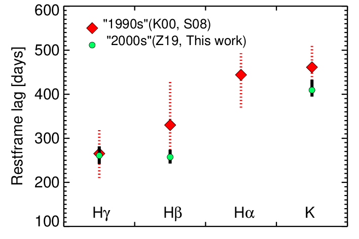
However, the difference between dust lag and BLR lags is small, in particular for H. This may be explained – at least partly – in the bowl model by the foreshortening effect. While the dust lag suffers from a strong foreshortening effect, the foreshortening of the BLR echo depends on how much above the equatorial plane the BLR clouds are located inside the bowl (Fig. 14, left). The similarity of the H lag with the dust lag suggests that H emitting gas lies close to the dust emitting bowl rim, in front of the rim as seen from the AD. We come back to that interesting possibility in Sect. V.2. Alternatively, one would have to take the much smaller BLR lags derived after a detrending (of the optical continuum light curves), e.g. H d (Zhang et al. 2019). We note that the dust lags essentially remain unchanged, if a detrending is applied, as we checked with several tests. A detailed investigation of these issues will be presented in a forthcoming paper.
Finally we note a direct consequence of the dust torus geometry for cosmological applications. For the nearby Sy-1 NGC 4151 Hönig et al. 2014 calculated a dust-parallax distance, based on dust RM data and interferometric size measurements. Likewise the GRAVITY Collaboration et al. 2019 tried that for three AGN (Mrk 335, Mrk 509 and NGC 3783), however with an extreme scatter. If the bowl model is true, then the lags should be converted to real , taking also into account the inclination of the bowl.66 6 For a bowl model at fixed and range, the dust lag strongly increases with inclination, e.g. for and the (simple geometric) TFs yield , because the TF is dominated by that side of the bowl, which is tilted away from the observer. This questions a widely made assumption (Hönig et al. 2014): “For reverberation mapping, however, inclination only broadens or smooths the time lag signal symmetrically around the mean without a significant shift in .” Nevertheless, NGC 4151 lies at , so that in the bowl model and the derived parallax distance should be correct. Im principle, parallax distances could be derived for 3C 273 as well, but we think that the uncertainty of the current data is by far too large for allowing a reliable angular distance calculation.
V.2 On the lag–luminosity relation
Figure 17 (top) shows the lag–luminosity diagram for two different NIR dust RM data sets, one from our OCA campaigns and one from the MAGNUM observations (Koshida et al. 2014; Minezaki et al. 2019), henceforth denoted with K14 and M19.
The analysed and published dust RM observations from OCA are on four sources (PGC 50427, WPVS 48, 3C 120, and 3C 273). All lags refer to . WPVS 48 was observed during two independent campaigns in 2013 and 2014 yielding – within the errors – the same lags (Pozo Nuñez et al. 2014; Figaredo 2018); here we take the average lag. Our dust reverberation campaign of 3C 120 took place in 2014 – 2015, one year after the factor 3 brightness outburst in 2013 which lasted until 2016 (Ramolla et al. 2015; Ramolla et al. 2018). Within the short time span between the begin of the outburst and our reverberation campaign, the dust geometry might not have changed significantly and any large size changes are unlikely. Therefore, we corrected the luminosity measured in 2014 – 2015 down by factor 3 to match the luminosity before the outburst. Table 5 lists the rest frame lags and luminosities used. A linear fit to the four sources (blue data points in Fig. 17, top) yields a slope for the lag–luminosity relation. For comparison, the black dashed line marks a slope with , which is widely adopted (Barvainis 1987; Koshida et al. 2014; Yoshii et al. 2014; Minezaki et al. 2019).
Fig. 17 shows also the MAGNUM dust reverberation data from K14 and M19 as red squares and stars, respectively. These lags were derived using the JAVELIN software (Zu et al. 2011); while JAVELIN lags are basically similar to other CCF lags, we do not know whether a bias could be present and therefore we here consider the MAGNUM lags separately from the OCA lags. The MAGNUM sample comprises 41 sources, 17 sources from K14 and 24 sources from M19, making it the largest homogeneously obtained dust RM set. All data are re-analysed by M19; we used the observed lags from their Table 3 column 3 (labeled , the optical – NIR power-law index of the AD) and their Table 6, and corrected the observed lags for time dilation . Strikingly, a linear fit to these MAGNUM data (all red points) yields a slope . In Figure 17 are also shown the residuals (data/fit); bottom: left for slope 0.5, right for slope 0.34. Fitting all MAGNUM and OCA sources together yields a slope . A fit excluding the three sources with erg/s yields . Thus, the slope is not biased by a few luminous sources.77 7 In their paper on the C IV 1549 lag-luminosity relation, Koratkar & Gaskell 1991a noticed the exceptional position of 3C 273 with respect to a slope (see their Fig. 1). In that paper, 3C 273 was the only source at the luminous end of the relation. A simple check on the reliability of a relation is to remove the four extremes, each one at the top, bottom, left and right of the diagram. Consequently, to bring the position of this single source into agreement with , they suggested that the luminosity of 3C 273 is an outlier and could be enhanced by beaming of continuum associated with the radio source. This possibility can largely be ruled out here, with the help of the two additional luminous radio-quiet sources in the sample of M19 (Fig. 17).


When observing in a fixed NIR band, the rest-frame wavelength of the observed dust emission becomes shorter at larger redshifts. In an attempt to account for this, Minezaki et al. 2019 derived a sophisticated wavelength-dependent correction for the lags, by multiplying with a redshift term . These wavelength-dependent corrected rest frame lags are listed in their Table 3 column 6. In the lag–luminosity diagram (Fig. 18) the lags become larger than without that correction (Fig. 17). The correction shifts the luminous sources more upwards, because they are typically at higher redshift (up to ) than the low luminosity sources. We applied the correction also to our OCA data, shown with blue colors in Fig. 18. The fitted slope of 0.33 0.01 remains about the same as without correction, because all OCA sources are at small redshift (). We fitted the corresponding lag–luminosity relation for the different data sets, yielding slopes of (for K14 only), (for M19 only), (for the combined K14 and M19 data), and (for the combined OCA and MAGNUM data). These slopes are steeper than without the wavelength-dependent correction, but significantly (at the level) shallower than the slope 0.5. At the high luminosity range ( erg/s), 3C 273 shows a relatively small lag compared to the two other quasars (PG 0953414, SDSS J09570023) but within the scatter (see residual plot bottom right of Fig. 18). Minezaki et al. 2019 already noticed the exceptional position of 3C 273 based on the lags by Soldi et al. 2008 and tentatively attributed it to the radio loudness of 3C 273. However, the two other quasars are radio quiet and a luminosity enhancement by the optical emission of a radio component does not explain the shallow slopes.
A matter of a debate is the wavelength dependence of the dust reverberation lag, here considered versus the optical bands, most commonly the or band. While the band is more sensitive to hotter dust than the and bands, it appears reasonable to expect a mix of hot dust temperatures for each spatial location (Oknyansky et al. 2015). There is no doubt that mid-infrared (MIR) lags are longer than NIR lags, which led to the common interpretation that the cooler dust emission arises from larger distance to the central heating source. Several groups found a longer lag at ( m) or ( m) compared to the or band, e.g. Glass 2004; Figaredo et al. 2018; Lyu et al. 2019. Based on sophisticated modeling of very sparse WISE observations Lyu et al. 2019 report a lag ratio , while Figaredo et al. 2018 find for the Seyfert WPVS 48 employing the combination of ground based and monitoring, Notably, neither Glass 2004 nor Figaredo et al. 2018 found significant differences in the lags between rest frame 1 and 2 m; typically any NIR lag differences are less than 5% of the optical-NIR lag and not significant at the level. The same holds for several other AGN with dust lags jointly determined in . Therefore, we believe that the wavelength-dependent lag correction applied by M19 should be adopted with care. In any case, both the OCA and MAGNUM data indicate a shallow slope between 0.33 and 0.4. This questions the widely adopted lag–luminosity slope of 0.5.
| Object | z | [days] | [erg/s] |
|---|---|---|---|
| PGC 50427 | 0.024 | ||
| WPVS 48 | 0.037 | ||
| 3C 120 | 0.033 | ||
| 3C 273 | 0.158 |
∗ brightness reduced by factor 3 to get the pre-outburst luminosity
The red data points show a large scatter around the fitted lag–luminosity relation (red line in Fig. 17). In the frame of the bowl model this could – at least partly – be understood as an effect of the inclination: If the dust emission originates in general from the edge of the bowl rim and if the AGN have different inclinations, then the TFs show a spread in shapes and asymmetries. For large inclination, the TF becomes dominated by that side of the bowl, which is tilted away from the observer (Figure 14,left). This will shift the measured lags to larger values between optical and NIR light curves. In parallel, for large inclination () , one may expect that the observer’s line-of-sight to the central AD crosses more absorbing material so that the luminosity may be reduced, compared to inclination (face-on view). Together, in the lag–luminosity plot, the source will shift up and left from the actual relation, inevitably leading to a scatter in the observed lag–luminosity data points. To reduced the scatter, it would be desirable to obtain via bowl modeling of the data a relation between and , provided the data are of sufficient quality. We suggest that the scatter in such a size–luminosity relation may be reduced. This is essential for cosmological applications like quasar distance estimates (Kobayashi et al. 1998; Oknyanskij 1999; Yoshii 2002; Yoshii et al. 2014; Hönig 2014; Minezaki et al. 2019).
In search for possible explanations for a shallow R-L slope, one possibibilty could be that luminosity-dependent internal extinction plays a role. Gaskell et al. 2004 derived the reddening curve for AGN. From the examined data sets they also found that, on average, low luminosity AGN ( erg/s) are redder and suffer from larger extinction (mag) than high luminosity AGN ( erg/s), see their Figure 5. Then in the R-L relation an intrinsic slope could be tilted to a shallower slope like the one we have observed here. While this is an elegant straight forward explanation, it is worth to have a closer look. If the extinction of Seyfert-1 nuclei is as large as mag and occurs in a screen between the BLR and the observer, then one would expect to see its signature also in the Balmer line decrement. With a few individual exceptions, however, the flux ratio, , of the broad H and H lines of both quasars and Seyfert-1s lies in the typical range about , so that screen extinction of mag in Seyfert-1s may be unlikely, hence rejecting simply screen extinction. Then the case of mixed extinction remains, where the absorbing dust has to be mixed with the BLR emitting gas, and the extinction affects essentially the background emission, which in our case is the continuum emission from the AD. For mixed extinction – likewise as in the presence of scattering material (Krügel 2009) – the amount of extinction is mostly underestimated, because the dust–gas mixture is considered only to small optical depths (, here not to confuse with the lag ). Then this surface treatment of the Balmer line decrement mimicks a smaller than real extinction. However, in case of such strong mixed extinction, the Balmer lags are expected to be similar to the hot dust lags, contrary to the lags observed for Seyfert-AGN so far. Another check of a high nuclear extinction in Seyfert-1s may be offered by the Flux Variation Gradients (like the ones shown in Fig. 4). They measure the continuum slope at wavelengths around the blue bump but so far do not show any luminosity dependence (Winkler et al. 1992). Future studies are needed to clarify these issues.
Finally we address two more possible lines for explaining the shallow lag–luminosity slope between 0.33 and 0.4.
1) Strömgren-behaviour: We consider the case that the lag–luminosity relation implies a relation between luminosity and the sublimation radius where slope (and is the speed of light and is a scaling factor). The relation with slope is strikingly reminiscent to the well known size–luminosity relation for H II regions, where (Strömgren 1939; McCullough 2000). The analogy between and is as follows:
For H II regions the Strömgren radius describes up to which distance from the ionising star the radiation field is strong enough to ionize, e.g. the hydrogen atoms. Beyond the radiation field is too weak so that the atoms “survive” unaffected. The reason for the slope for the Strömgren relation is that interjacent material inside absorbs the radiation from the ionising star.
For the dust in AGN we deal with the sublimation radius . Inside of the AGN radiation field is sufficiently strong, so that the dust grains evaporate (in analogy to become ionized). Outside of the radiation field is too weak so that the dust grains can survive. So far, the assumption was made that the (dust heating UV) photons of the AD travel all the way until without being absorbed by interjacent material. This led to the widely adopted relation . However, if sufficient absorbing material lies between the AD and the dust grains, then becomes smaller, and this will lead to a shallower slope . Then the slope found in Figs. 17 and 18 implies that there is in fact plenty of absorbing material between the AD and the dust grains. This means for the bowl model considered here, that even the line between the AD and the bowl edge at crosses a significant amount of absorbing material. The large H lag / dust lag mentioned in Sect. V.1 may hint to such material.
2) Geometric effects of a bowl mirror: We assume a bowl model with fixed half opening angle 45∘ irrespective of the AD luminosity. Clearly, both the bowl rim and material inside the bowl act in the net effect like a reflecting mirror for the photons from the AD. The photons are scattered by electrons and dust grains. In addition, reprocessed continuum emission may play a role; for instance Chelouche et al. 2019 found evidence of a non-disk optical continuum emission around AGN, which likely comes from the inner wall of the BLR. Thus, the observer sees – in addition to the AD flux – also a contribution from scattered or reprocessed photons. This leads to an amplification of the original AD brightness. The relative amplification may be small (a few percent) but it is worth to consider how far it is luminosity dependent. We make the assumption that the bowl opening angle and the geometric covering angle for intercepting AD photons is luminosity independent. Then the effect of the bowl rim on might be scale-invariant. However, the volume inside the bowl increases proportional to . If the density of scattering or reprocessing particles inside the bowl is independent of the AD luminosity, then one may expect that . This yields . Assuming for simplicity we get . In other words, in the net effect the actual luminosity of the AD may be overestimated by a factor which scales with . Then in the lag–luminosity relation the data points will be shifted to large values, so that the resulting slope becomes shallower than .
A detailed quantitative consideration of the potential Strömgren-like behaviour of AGN and the geometric effects of a bowl mirror will be presented in a future paper.
VI Summary and conclusions
We performed a 5 years reverberation mapping campaign of 3C 273 in the optical () and NIR () bands at the Bochum University Observatory near Cerro Armazones (OCA). The optical light curves were supplemented by longer and denser sampled band light curves from Zhang et al. 2019. The results are:
- 1.
To obtain the pure dust light curves, the contribution of host galaxy and accretion disk to the NIR bands had to be removed. The resulting dust light curves show consistently correlated variations in all three NIR bands, giving confidence that the procedure worked well to remove the contribution of host galaxy and accretion disk.
- 2.
For all three filter pairs (, , ) the color temperatures change by about 5% (i.e. a factor 1.05) between the bright and faint states. On the other hand, the amplitudes of the dust light curves increase with decreasing wavelength from 0.2 at to 0.4 in . Because the filters measure the dust emission on the Wien tail of the Planck function, the brightness changes are expected to become larger at shorter wavelengths; they may exceed the amplitude of the triggering signal light curve. This altogether consistently indicates that the variations of the dust emission are likely due to (mean) temperature changes of the dust grains in the order of 5%.
- 3.
We derived the dust covering factor from the optical/UV and NIR luminosities, yielding small values 8%, consistent with the results 7% for other type-1 AGN by Landt et al. 2011.
- 4.
We determined the time lag of the dust light curves against the -light curve trough different CCF methods and found an average time lag of d. Some correlation methods reveal an interesting asymmetry, which is consistent with the transfer function of a tilted dust geometry.
- 5.
We re-analysed the data of Soldi et al. 2008 and compared the dust time lag and CCF asymmetries during our observing campaign and theirs.
- 6.
The average time lag of d is a factor of smaller than expected from the interferometric ring radius of ld. Interferometry measures the projected size as seen by the observer, while RM measures the 3-dimensional light travel time difference in the system. We suggest that the difference between interferometric size and RM lags can be explained by 3D geometrical effects, in particular the foreshortening effect from which the reverberation data suffer.
- 7.
To bring the observational findings into a consistent picture, we considered a bowl shaped torus geometry as proposed by Goad et al. 2012, where the dust emission originates from the edge of the bowl rim with a small covering angle , as justified by the small . We used an inclination angle of indicated from radio jet studies (Lobanov & Zensus 2001; Savolainen et al. 2006; Jorstad et al. 2017). For such a model with an equatorial size ld the (simple geometric) transfer function (TF) is double-horned and yields an asymmetric cross correlation similar to that found from the data. We have convolved different TFs for a bowl geometry with the host-subtracted band light curve and showed the corresponding echo light curves. For an equatorial size ld, the echo light curve delays are in agreement with the delays found in our data, and the modeled cross correlations show an asymmetry similar to that observed in the CCF. The main conclusion from our study is that the hot dust emission seen in the NIR originates from a tilted () thin ring which lies above the equatorial plane.
- 8.
The relation between dust lag and optical luminosity shows a large scatter. To reduce the scatter for future cosmological applications, it may be desirable to obtain via modeling of the data (provided they are of sufficient quality) and check for a relation between and .
- 9.
We find for the lag–luminosity relation a rather shallow slope between 0.33 and 0.4. This rejects the widely adopted slope 0.5 at the 3-sigma level. We envisage three possible explanations for the shallow slope:
1) Gaskell et al. 2004 found that the internal extinction in AGN increases with decreasing AGN luminosity by mag between quasars and Seyferts. If the internal extinction in AGN is in fact so high and shows such a strong luminosity dependence, then the slope may be tilted from 0.5 to about 0.33.
2) AGN have a similar behaviour as H II regions where the size of the ionized region . If a substantial amount of absorbing material lies between the AD and the dust grains, this allows for a shortened dust sublimation radius. If the material density is -invariant, the relative shortening increases with the path length between AD and dust. The path length (bowl size) depends on . Then, in the lag–luminosity diagram, the relative reduction of the lag increases with .
3) The observer measures an AD luminosity which is magnified by scattered and reprocessed radiation from material in the bowl, and the relative contribution of this magnification of increases with the volume of the bowl and therefore also with . Then, in the lag–luminosity diagram, the relative overestimation of increases with .
While these findings apply to the single case of the luminous quasar 3C 273, future detailed studies on a larger quasar sample should be envisaged to corroborate the conclusions.
References
- Alexander (1997) Alexander, T. 1997, Astrophysics and Space Science Library, Vol. 218, Is AGN Variability Correlated with Other AGN Properties? ZDCF Analysis of Small Samples of Sparse Light Curves, ed. D. Maoz, A. Sternberg, & E. M. Leibowitz, 163, doi: 10.1007/978-94-015-8941-3_14
- Antonucci (1993) Antonucci, R. 1993, ARA&A, 31, 473, doi: 10.1146/annurev.aa.31.090193.002353
- Bahcall et al. (1997) Bahcall, J. N., Kirhakos, S., Saxe, D. H., & Schneider, D. P. 1997, ApJ, 479, 642, doi: 10.1086/303926
- Bahcall et al. (1972) Bahcall, J. N., Kozlovsky, B.-Z., & Salpeter, E. E. 1972, ApJ, 171, 467, doi: 10.1086/151300
- Barthel (1989) Barthel, P. D. 1989, ApJ, 336, 606, doi: 10.1086/167038
- Barvainis (1987) Barvainis, R. 1987, ApJ, 320, 537, doi: 10.1086/165571
- Bentz et al. (2013) Bentz, M. C., Denney, K. D., Grier, C. J., et al. 2013, ApJ, 767, 149, doi: 10.1088/0004-637X/767/2/149
- Bertin (2006) Bertin, E. 2006, Astronomical Society of the Pacific Conference Series, Vol. 351, Automatic Astrometric and Photometric Calibration with SCAMP, ed. C. Gabriel, C. Arviset, D. Ponz, & S. Enrique, 112
- Bertin et al. (2002) Bertin, E., Mellier, Y., Radovich, M., et al. 2002, Astronomical Society of the Pacific Conference Series, Vol. 281, The TERAPIX Pipeline, ed. D. A. Bohlender, D. Durand, & T. H. Handley, 228
- Bochkarev & Gaskell (2009) Bochkarev, N. G., & Gaskell, C. M. 2009, Astronomy Letters, 35, 287, doi: 10.1134/S1063773709050016
- Bock et al. (2000) Bock, J. J., Neugebauer, G., Matthews, K., et al. 2000, AJ, 120, 2904, doi: 10.1086/316871
- Braatz et al. (1993) Braatz, J. A., Wilson, A. S., Gezari, D. Y., Varosi, F., & Beichman, C. A. 1993, ApJ, 409, L5, doi: 10.1086/186846
- Cameron et al. (1993) Cameron, M., Storey, J. W. V., Rotaciuc, V., et al. 1993, ApJ, 419, 136, doi: 10.1086/173467
- Chang et al. (2006) Chang, R., Shen, S., Hou, J., Shu, C., & Shao, Z. 2006, MNRAS, 372, 199, doi: 10.1111/j.1365-2966.2006.10826.x
- Chelouche et al. (2019) Chelouche, D., Pozo Nuñez, F., & Kaspi, S. 2019, Nature Astronomy, 3, 251, doi: 10.1038/s41550-018-0659-x
- Chelouche et al. (2017) Chelouche, D., Pozo-Nuñez, F., & Zucker, S. 2017, ApJ, 844, 146, doi: 10.3847/1538-4357/aa7b86
- Cherepashchuk & Lyutyi (1973) Cherepashchuk, A. M., & Lyutyi, V. M. 1973, Astrophys. Lett., 13, 165
- Choloniewski (1981) Choloniewski, J. 1981, Acta Astron., 31, 293
- Clavel et al. (1989) Clavel, J., Wamsteker, W., & Glass, I. S. 1989, ApJ, 337, 236, doi: 10.1086/167100
- Czerny & Hryniewicz (2011) Czerny, B., & Hryniewicz, K. 2011, A&A, 525, L8, doi: 10.1051/0004-6361/201016025
- Czerny et al. (2017) Czerny, B., Li, Y.-R., Hryniewicz, K., et al. 2017, ApJ, 846, 154, doi: 10.3847/1538-4357/aa8810
- Czerny et al. (2019) Czerny, B., Wang, J.-M., Du, P., et al. 2019, ApJ, 870, 84, doi: 10.3847/1538-4357/aaf396
- Dibai (1977) Dibai, E. A. 1977, Soviet Astronomy Letters, 3, 1
- Du et al. (2016) Du, P., Lu, K.-X., Zhang, Z.-X., et al. 2016, ApJ, 825, 126, doi: 10.3847/0004-637X/825/2/126
- Edelson & Krolik (1988) Edelson, R. A., & Krolik, J. H. 1988, ApJ, 333, 646, doi: 10.1086/166773
- Figaredo (2018) Figaredo, C. S. 2018, Master’s thesis, Ruhr-Universität Bochum, Bochum, Germany
- Figaredo et al. (2018) Figaredo, C. S., Nuñez, F. P., Ramolla, M., et al. 2018, in Revisiting Narrow-Line Seyfert 1 Galaxies and their Place in the Universe, 57
- Fukugita et al. (1995) Fukugita, M., Shimasaku, K., & Ichikawa, T. 1995, PASP, 107, 945, doi: 10.1086/133643
- Gaskell et al. (2019) Gaskell, C. M., Bartel, K., Deffner, J. N., & Xia, I. 2019, arXiv e-prints, arXiv:1909.06275. https://arxiv.org/abs/1909.06275
- Gaskell et al. (2004) Gaskell, C. M., Goosmann, R. W., Antonucci, R. R. J., & Whysong, D. H. 2004, ApJ, 616, 147, doi: 10.1086/423885
- Gaskell et al. (2007) Gaskell, C. M., Klimek, E. S., & Nazarova, L. S. 2007, arXiv e-prints, arXiv:0711.1025. https://arxiv.org/abs/0711.1025
- Gaskell & Sparke (1986) Gaskell, C. M., & Sparke, L. S. 1986, ApJ, 305, 175, doi: 10.1086/164238
- Glass (2004) Glass, I. S. 2004, MNRAS, 350, 1049, doi: 10.1111/j.1365-2966.2004.07712.x
- Goad et al. (2012) Goad, M. R., Korista, K. T., & Ruff, A. J. 2012, MNRAS, 426, 3086, doi: 10.1111/j.1365-2966.2012.21808.x
- GRAVITY Collaboration et al. (2019) GRAVITY Collaboration, Dexter, J., Shangguan, J., et al. 2019, arXiv e-prints, arXiv:1910.00593. https://arxiv.org/abs/1910.00593
- Haas et al. (2011) Haas, M., Chini, R., Ramolla, M., et al. 2011, A&A, 535, A73, doi: 10.1051/0004-6361/201117325
- Haas et al. (2012) Haas, M., Hackstein, M., Ramolla, M., et al. 2012, Astronomische Nachrichten, 333, 706, doi: 10.1002/asna.201211717
- Hodapp et al. (2010) Hodapp, K. W., Chini, R., Reipurth, B., et al. 2010, Society of Photo-Optical Instrumentation Engineers (SPIE) Conference Series, Vol. 7735, Commissioning of the infrared imaging survey (IRIS) system, 77351A, doi: 10.1117/12.856288
- Hönig (2014) Hönig, S. F. 2014, ApJ, 784, L4, doi: 10.1088/2041-8205/784/1/L4
- Hönig et al. (2014) Hönig, S. F., Watson, D., Kishimoto, M., & Hjorth, J. 2014, Nature, 515, 528, doi: 10.1038/nature13914
- Hönig et al. (2013) Hönig, S. F., Kishimoto, M., Tristram, K. R. W., et al. 2013, ApJ, 771, 87, doi: 10.1088/0004-637X/771/2/87
- Horne et al. (2004) Horne, K., Peterson, B. M., Collier, S. J., & Netzer, H. 2004, PASP, 116, 465, doi: 10.1086/420755
- Huchra & Burg (1992) Huchra, J., & Burg, R. 1992, ApJ, 393, 90, doi: 10.1086/171488
- Jarrett et al. (2019) Jarrett, T. H., Cluver, M. E., Brown, M. J. I., et al. 2019, ApJS, 245, 25, doi: 10.3847/1538-4365/ab521a
- Jorstad et al. (2017) Jorstad, S. G., Marscher, A. P., Morozova, D. A., et al. 2017, ApJ, 846, 98, doi: 10.3847/1538-4357/aa8407
- Kabath et al. (2009) Kabath, P., Erikson, A., Rauer, H., et al. 2009, A&A, 506, 569, doi: 10.1051/0004-6361/200911909
- Kaspi et al. (2000) Kaspi, S., Smith, P. S., Netzer, H., et al. 2000, ApJ, 533, 631, doi: 10.1086/308704
- Kawaguchi & Mori (2010) Kawaguchi, T., & Mori, M. 2010, ApJ, 724, L183, doi: 10.1088/2041-8205/724/2/L183
- Kawaguchi & Mori (2011) —. 2011, ApJ, 737, 105, doi: 10.1088/0004-637X/737/2/105
- Kishimoto et al. (2005) Kishimoto, M., Antonucci, R., & Blaes, O. 2005, MNRAS, 364, 640, doi: 10.1111/j.1365-2966.2005.09577.x
- Kishimoto et al. (2008) Kishimoto, M., Antonucci, R., Blaes, O., et al. 2008, Nature, 454, 492, doi: 10.1038/nature07114
- Kishimoto et al. (2011) Kishimoto, M., Hönig, S. F., Antonucci, R., et al. 2011, A&A, 527, A121, doi: 10.1051/0004-6361/201016054
- Kishimoto et al. (2009) —. 2009, A&A, 507, L57, doi: 10.1051/0004-6361/200913512
- Kishimoto et al. (2007) Kishimoto, M., Hönig, S. F., Beckert, T., & Weigelt, G. 2007, A&A, 476, 713, doi: 10.1051/0004-6361:20077911
- Kobayashi et al. (1998) Kobayashi, Y., Yoshii, Y., Peterson, B. A., et al. 1998, Society of Photo-Optical Instrumentation Engineers (SPIE) Conference Series, Vol. 3352, MAGNUM (multicolor active galactic nuclei monitoring) Project, ed. L. M. Stepp, 120–128, doi: 10.1117/12.319247
- Koratkar & Gaskell (1991a) Koratkar, A. P., & Gaskell, C. M. 1991a, ApJ, 370, L61, doi: 10.1086/185977
- Koratkar & Gaskell (1991b) —. 1991b, ApJS, 75, 719, doi: 10.1086/191547
- Koshida et al. (2014) Koshida, S., Minezaki, T., Yoshii, Y., et al. 2014, ApJ, 788, 159, doi: 10.1088/0004-637X/788/2/159
- Kruegel (2003) Kruegel, E. 2003, The physics of interstellar dust
- Krügel (2009) Krügel, E. 2009, A&A, 493, 385, doi: 10.1051/0004-6361:200809976
- Landt et al. (2011) Landt, H., Elvis, M., Ward, M. J., et al. 2011, MNRAS, 414, 218, doi: 10.1111/j.1365-2966.2011.18383.x
- Lobanov & Zensus (2001) Lobanov, A. P., & Zensus, J. A. 2001, Science, 294, 128, doi: 10.1126/science.1063239
- Lyu et al. (2019) Lyu, J., Rieke, G. H., & Smith, P. S. 2019, ApJ, 886, 33, doi: 10.3847/1538-4357/ab481d
- McCullough (2000) McCullough, P. R. 2000, PASP, 112, 1542, doi: 10.1086/317718
- Minezaki et al. (2019) Minezaki, T., Yoshii, Y., Kobayashi, Y., et al. 2019, ApJ, 886, 150, doi: 10.3847/1538-4357/ab4f7b
- Neugebauer & Matthews (1999) Neugebauer, G., & Matthews, K. 1999, AJ, 118, 35, doi: 10.1086/300945
- Oknyanskij (1999) Oknyanskij, V. L. 1999, Odessa Astronomical Publications, 12, 99
- Oknyansky et al. (2015) Oknyansky, V. L., Gaskell, C. M., & Shimanovskaya, E. V. 2015, Odessa Astronomical Publications, 28, 175. https://arxiv.org/abs/1511.02170
- Oknyansky et al. (2018) Oknyansky, V. L., Malanchev, K. L., & Gaskell, C. M. 2018, in Revisiting Narrow-Line Seyfert 1 Galaxies and their Place in the Universe, 12. https://arxiv.org/abs/1810.08844
- Patat et al. (2011) Patat, F., Moehler, S., O’Brien, K., et al. 2011, A&A, 527, A91, doi: 10.1051/0004-6361/201015537
- Penston (1991) Penston, M. V. 1991, in Variability of Active Galactic Nuclei, ed. H. R. Miller & P. J. Wiita, 343
- Peterson (1993) Peterson, B. M. 1993, PASP, 105, 247, doi: 10.1086/133140
- Peterson et al. (1998) Peterson, B. M., Wanders, I., Horne, K., et al. 1998, PASP, 110, 660, doi: 10.1086/316177
- Pozo Nuñez et al. (2014) Pozo Nuñez, F., Haas, M., Chini, R., et al. 2014, A&A, 561, L8, doi: 10.1051/0004-6361/201323178
- Pozo Nuñez et al. (2015) Pozo Nuñez, F., Ramolla, M., Westhues, C., et al. 2015, A&A, 576, A73, doi: 10.1051/0004-6361/201525910
- Ramolla et al. (2015) Ramolla, M., Pozo Nuñez, F., Westhues, C., Haas, M., & Chini, R. 2015, A&A, 581, A93, doi: 10.1051/0004-6361/201526846
- Ramolla et al. (2013) Ramolla, M., Drass, H., Lemke, R., et al. 2013, Astronomische Nachrichten, 334, 1115, doi: 10.1002/asna.201311912
- Ramolla et al. (2016) Ramolla, M., Westhues, C., Hackstein, M., et al. 2016, Society of Photo-Optical Instrumentation Engineers (SPIE) Conference Series, Vol. 9911, A green observatory in the Chilean Atacama desert, 99112M, doi: 10.1117/12.2234018
- Ramolla et al. (2018) Ramolla, M., Haas, M., Westhues, C., et al. 2018, A&A, 620, A137, doi: 10.1051/0004-6361/201732081
- Sakata et al. (2010) Sakata, Y., Minezaki, T., Yoshii, Y., et al. 2010, ApJ, 711, 461, doi: 10.1088/0004-637X/711/1/461
- Savolainen et al. (2006) Savolainen, T., Wiik, K., Valtaoja, E., & Tornikoski, M. 2006, A&A, 446, 71, doi: 10.1051/0004-6361:20053753
- Schlafly & Finkbeiner (2011) Schlafly, E. F., & Finkbeiner, D. P. 2011, ApJ, 737, 103, doi: 10.1088/0004-637X/737/2/103
- Soldi et al. (2008) Soldi, S., Türler, M., Paltani, S., et al. 2008, A&A, 486, 411, doi: 10.1051/0004-6361:200809947
- Strömgren (1939) Strömgren, B. 1939, ApJ, 89, 526, doi: 10.1086/144074
- Suganuma et al. (2006) Suganuma, M., Yoshii, Y., Kobayashi, Y., et al. 2006, ApJ, 639, 46, doi: 10.1086/499326
- Tomita et al. (2006) Tomita, H., Yoshii, Y., Kobayashi, Y., et al. 2006, ApJ, 652, L13, doi: 10.1086/509878
- Winkler et al. (1992) Winkler, H., Glass, I. S., van Wyk, F., et al. 1992, MNRAS, 257, 659, doi: 10.1093/mnras/257.4.659
- Wold et al. (2010) Wold, I., Sheinis, A. I., Wolf, M. J., & Hooper, E. J. 2010, MNRAS, 408, 713, doi: 10.1111/j.1365-2966.2010.17163.x
- Xiong et al. (2017) Xiong, D., Bai, J., Zhang, H., et al. 2017, ApJS, 229, 21, doi: 10.3847/1538-4365/aa64d2
- Yoshii (2002) Yoshii, Y. 2002, in New Trends in Theoretical and Observational Cosmology, ed. K. Sato & T. Shiromizu, 235
- Yoshii et al. (2014) Yoshii, Y., Kobayashi, Y., Minezaki, T., Koshida, S., & Peterson, B. A. 2014, ApJ, 784, L11, doi: 10.1088/2041-8205/784/1/L11
- Zhang et al. (2019) Zhang, Z.-X., Du, P., Smith, P. S., et al. 2019, ApJ, 876, 49, doi: 10.3847/1538-4357/ab1099
- Zu et al. (2011) Zu, Y., Kochanek, C. S., & Peterson, B. M. 2011, ApJ, 735, 80, doi: 10.1088/0004-637X/735/2/80
Appendix A Different Cross Correlation Functions


