The Composition, Excitation, and Physical State of Atomic Gas in the Debris Disk Surrounding 51 Oph (catalog ) Based on observations with the NASA/ESA Hubble Space Telescope obtained from the Data Archive at the Space Telescope Science Institute, which is operated by the Associations of Universities for Research in Astronomy, Incorporated, under NASA contract NAS5-26555. ©2020. The American Astronomical Society. All rights reserved.Facilities: HST (STIS, GHRS), FUSE, HUT, VLT:Kueyen (UVES)Owens, developed by Martin Lemoine (Institut d’Astrophysique de Paris) and the French FUSE Science Team
Abstract
We measured 304 absorption features in the ultraviolet and visible spectra of the star 51 Oph, which is known to have a debris disk with a high inclination. We analyzed the relative populations of atoms in excited fine-structure and metastable levels that are maintained by optical pumping and collisional excitation by electrons, and we found that most of the gas is situated at about 6 AU from the star, has an electron volume density , and a temperature K. Our interpretations reveal that the gas is partly ionized, has a column density of neutral hydrogen equal to , and has a composition similar to that of a mildly depleted interstellar medium or that of Jupiter-family comets. Compared to results for disks around some other stars, such as Pic and 49 Cet, we find surprisingly little neutral carbon. No molecular features were detected, which indicates that our line of sight misses the molecule-rich central plane of the disk. The tilt of the disk is also validated by our being able to detect resonant scattering of the starlight by oxygen atoms.
Keywords:
Circumstellar gas (238), Circumstellar matter (241), Circumstellar disks (235), Abundance ratios (11), Debris disks (363)I Introduction
The emergence and growth in our understanding of gas and dust in orbit around stars that are approaching or are on the main sequence has been an important new endeavor for both observers and theoreticians (as reviewed by Hughes et al. 2018). This topic has also provided a critical link to our knowledge on the formation of extrasolar planets (Vidal-Madjar et al. 1998 ; Wyatt 2018) and alterations of element abundances in some stellar atmospheres, such as those of white dwarf stars (Jura & Young 2014). Discoveries from orbiting observatories, such as the Infrared Space Observatory (ISO), Spitzer Space Telescope, Wide Field Infrared Survey Explorer (WISE), and Herschel Space Observatory have revealed that approximately 20% of both A-type and the F, G, and K-type stars near the main sequence exhibit measurable excesses of infrared emission11 1 An unbiased survey of A-type stars by Thureau et al. (2014) indicates a somewhat higher percentage, ranging between 21 and 54%. A study by Moór et al. (2017) of A-type stars with dust-rich disks revealed that 11 out of 16 of them exhibited measurable CO emission. that are well above an extrapolation of the Rayleigh-Jeans tails for the radiation from the stellar photospheres (Wyatt 2018).
Coronagraphic, polarimetric, and interferometric observing facilities working at visible wavelengths (e.g., STIS on HST, SPHERE/ZIMPOL on the VLT, and the Keck nulling interferometer), as well as radio interferometers (ALMA, SMA, NOEMA, CARMA), the far infrared PACS instrument on the Herschel Space Observatory, and millimeter observations taken by SCUBA-2 on the JCMT have allowed us to obtain detailed information on the strengths and morphologies of the emissions by atoms, molecules, and dust surrounding the stars. There is an immense volume of literature covering these observations. There are also many publications that have highlighted the absorption features produced by Ca II, Na I and sometimes Fe I that appear at visible wavelengths in the spectra of the central stars. These species have even been imaged in emission for the iconic example of an edge-on disk around the star Pic (Olofsson et al. 2001 ; Brandeker et al. 2004).
If a central star is hot enough and close enough to provide a spectrum in the ultraviolet, an opportunity to detect with great sensitivity various atomic and molecular constituents in the circumstellar medium is presented. Intensive investigations of the matter surrounding Pic got underway with observations using the International Ultraviolet Explorer (IUE) (Kondo & Bruhweiler 1985 ; Lagrange et al. 1987 ; Lagrange-Henri et al. 1988 ; Lagrange-Henri et al. 1989). These early investigations highlighted the existence of atoms in a stable component at the velocity of the star, but in addition, there were occasional appearances of absorption components at significantly large positive velocities, which were interpreted as falling evaporating bodies (FEB) (Vidal-Madjar et al. 1998). The high frequency of detecting the FEB phenomenon has been interpreted to arise from perturbations by planets on the orbits of comet-sized objects (Karmann et al. 2001 ; Thébault & Beust 2001), which eventually plunge toward the star.
Following the era of IUE, observations with the Goddard High Resolution Spectrograph (GHRS) (Brandt et al. 1994) and Space Telescope Imaging Spectrograph (STIS) (Woodgate et al. 1998) aboard Hubble Space Telescope (HST), together with the Far Ultraviolet Spectroscopic Explorer (FUSE) (Moos et al. 2000 ; Sahnow et al. 2000), provided a vast improvement in the number and quality of the results. Absorption features associated with the debris disk of Pic have been the most intensively studied ones, but to lesser degrees, there have been interpretations of the spectra of other hot stars, such as 49 Cet (Malamut et al. 2014 ; Roberge et al. 2014 ; Miles et al. 2016 - STIS spectra), 51 Oph, HD 256, HD 42111 (Lecavelier des Etangs et al. 1997b - GHRS spectra only), 2 And (Cheng & Neff 2003 - FUSE and GHRS), Her (Chen & Jura 2003 - FUSE only), AB Aur (Roberge et al. 2001 - FUSE and STIS), and HD 109573 (upper limits only) (Chen & Kamp 2004 - FUSE and STIS), HD 32297 (marginal S/N) (Fusco et al. 2013), HD 141569 (Malamut et al. 2014), HD 163296 (Tilling et al. 2012 - STIS medium res. echelle) and HD 172555 (Grady et al. 2018 - STIS and COS).
The origin of gas accompanying debris disks is a fundamental problem: is it primordial, is it ejected from the star (and slowed down by some process), or – more likely – does it arise from the orbiting planetesimals, comets, or dust grains that are either evaporating atoms or liberating gas as they collide with each other? An examination of the relative abundances of different elements, which often differ appreciably from the solar abundances, can provide some guidance on this question (Xie et al. 2013).
A distinctive property of the UV absorption spectra of gas associated with debris disks is the appearance of features arising from many different excited fine-structure and metastable levels of various atoms and ions. The most conspicuous absorptions from levels of high excitation are those from Fe II, as we will illustrate later in Figure 2, which have radiative lifetimes ranging from 10 seconds to 50 hours (Quinet et al. 1996) and must be populated by radiation pumping and/or collisional excitations with electrons (the effects of collisions with neutral atoms and ions are small by comparison). For densities below the critical densities of the levels, there can be deviations from a straight-line relationship for the level populations in an excitation diagram ( vs. ), which in turn will reveal clues on the environmental parameters that are responsible for the excitations. Such deviations are clearly evident in this type of diagram for the Fe I level populations derived from a high-S/N spectrum of Pic at visible wavelengths (Vidal-Madjar et al. 2017).
Our current study is directed toward using absorption features in the ultraviolet to gain information on the gas constituents that surround the star 51 Oph. This Herbig Ae/Be star has been assigned a spectral classification B9.5Ve by Dunkin et al. (1997), and has the parameters (Jamialahmadi et al. 2015), K, , [M/H] = +0.10, and an estimated age (Montesinos et al. 2009). The distance to the star is 123 pc (Arenou et al. 2018 ; Luri et al. 2018). A spectral energy distribution with an infrared excess (Malfait et al. 1998), the presence of emissions at from silicates (Fajardo-Acosta et al. 1993 ; Meeus et al. 2001), from PAHs (Keller et al. 2008), several atomic excited atomic fine-structure levels (Meeus et al. 2012 ; Dent et al. 2013), and various gas-phase molecules (van den Ancker et al. 2001) all present clear evidence of gaseous and solid matter circulating around this star. We are not the first to study absorption features in the UV spectrum of this star, and we will refer to a number of previous investigations later in the paper. The UV spectrum of 51 Oph exhibits a rich assortment of lines from many different elements, and these elements have significant populations in those metastable levels that cannot undergo rapid radiative decays. We had the good fortune of locating relevant atomic data for N I, Fe II, and Ni II that allowed us to investigate in some detail the factors that governed the excited level populations.
II Data
Table 1 summarizes some key parameters of the observations. Nearly all of the conclusions in this paper are based on observations taken at ultraviolet wavelengths with the highest resolution echelle modes of STIS aboard HST. These data are supplemented by observations by the GHRS over very limited wavelength ranges. The spectra recorded by the GHRS are used only to make comparisons with STIS data to check for possible time variability of some spectral features. A limited number of absorption features relevant to our study appear at visible wavelengths. To measure such features, we made use of archived echelle spectra recorded by the Ultraviolet and Visual Echelle Spectrograph (UVES) (Dekker et al. 2000) on the Kueyen Very Large Telescope (VLT) operated by the European Southern Observatory.
Observations of 51 Oph in the far ultraviolet recorded by FUSE have been reported by Roberge et al. (2002). We confined our use of the FUSE spectra to probe only the elements N I, Cl II, P II and a metastable level of O I, which we could not measure in the STIS spectrum. Finally, we used a spectrum recorded by the Hopkins Ultraviolet Telescope (HUT) (Kruk et al. 1995 ; Dixon et al. 2013) to validate our choice of parameters for a theoretical stellar spectrum that we used to calculate the optical pumping of levels, as will be discussed later in Section VI.1.1.
| Instrument, Mode | Aperture | Resolution | Range | Observation |
|---|---|---|---|---|
| arc-sec | (Å) | Date | ||
| STIS E140H, E230H | 114,000 | 1280.51902.0 | 2003 May 26 | |
| 200,000 | 1879.52396.5 | |||
| 2576.52845.5 | ||||
| GHRS ECH-B | 0.25 | 100,000 | 2597.22610.0 | 1996 Feb 21 |
| 2793.32808.0 | ||||
| G160M | 20,000 | 1531.51567.5 | ||
| UVES CD#2 | 0.612 | 72,000 | 33004500 | 2007 MayAug |
| CD#3 | 46506650 | |||
| FUSE | 15,000 | 9921187 | 2001 Apr 29aaWe refrained from using exposures taken in 2000 with a larger entrance aperture. Also, various technical issues discussed by Roberge et al. (2002) made the reduction and interpretation of these earlier spectra less attractive. | |
| HUT | 20 | 500 | 8001850 | 1995 Mar 15 |
It is well established that absorption features arising from circumstellar gas can vary with time, with the appearance and disappearance of velocity-shifted features. A large collection of 51 Oph spectra recorded by the IUE satellite at different times show occasional appearances of features at very high negative and positive velocities, ranging from many tens of to as much as 100 (Grady & Silvis 1993). All of our observations with STIS were taken over a time interval of only two hours, so the possible influence of such variability is small. Nevertheless, we also made use of UVES spectra at visible wavelengths taken at a very different time for our analysis of Na I, Ca I, Ca II, Ti II, Cr II, Mn II, and Fe I.
To gain some indication that the features at low velocities that we studied here are not varying in time, we compared GHRS observations taken many years earlier than our STIS ones (see Table 1) and found no evidence of any significant changes in the appearances of the features. Figure 1 shows the close match of features in the GHRS and STIS spectra taken at nearly the same wavelength resolutions. Of course, this evidence is only circumstantial; we cannot rigorously rule out the existence of some variability that could cause features in the UVES spectra to not match those in the STIS ones. For instance, Roberge et al. (2002) reported some very small changes in some profile shapes that occurred between their two FUSE exposures separated by 6 days in 2000.
III Analysis of the Spectra
III.1 Absorption Features from Atomic Ground-State, Excited Fine-structure, and Metastable Levels
Table 7 in the appendix lists the different features that we analyzed in the UV and visible spectra of 51 Oph. Most were strong enough to appear well above the noise in the continuum level and could yield column density values, while others were so weak or invisible that we could obtain only upper limits to column densities using a procedure outlined below in Section III.2.
Features from the unexcited states of atoms probably have some contamination from absorption by the foreground interstellar medium, but all of the lines from the excited levels arise from just the circumstellar gas around 51 Oph. For the ground-state levels, we attempted to distinguish contributions from the foreground interstellar medium (ISM) from circumstellar ones, using the identifications of distinct radial velocity components as a guide, as we will discuss in Section IV. To accomplish this goal, we used the profile-fitting software called Owens.f that was developed in the 1990s by M. Lemoine and the French FUSE science team. To obtain a more coherent picture of the components, the analysis software allows us to fit simultaneously different lines from several energy levels and include several species in a single structure of velocity components. A solution emerges where all central velocities and turbulent velocity widths for all species of the same component are identical, but with thermal broadening widths that recognize the expected variations that change with atomic masses. In some cases, we sensed that two velocity components for purely circumstellar gas were partly resolved, but in others, only one was present.
Owens constructs trial theoretical profiles that are then convolved with the instrumental line spread function (LSF). The spectra have not been normalized to the stellar continuum; instead, the stellar profile is included in the fit as free parameters for an -degree polynomial ( is always 3 and often equal to 1). The LSFs appropriate for the echelle gratings E140H and E230H are tabulated in the STIS Instrument Handbook (Riley et al. 2018). For the observations of 51 Oph, E140H data (1460 Å to 1896 Å) were observed with the arc-sec aperture, and E230H data (1874 to 2846 Å) through the high-resolution slit with dimensions arc-sec. For both slits, the LSFs are composed of a broad and a narrow component whose full widths at half maxima (FWHM) are derived by performing a double-Gaussian fit to the tabulated LSFs. As a result, we adopted for the low-amplitude, broad component an FWHM of 4.9 pixels and 5.1 pixels for E140H and E230H data, respectively, and for the taller narrow component, an FWHM of 1.26 pixels for E140H and 1.45 pixels for E230H. For the UVES data, we have adopted a Gaussian LSF as specified by Figure 2.7 of the UVES User Manual (Sbordone & Ledoux 2019): FWHM = 2.4 pixels () for the blue side and FWHM = 3.5 pixels () for the red side.
The wavelength accuracy of STIS across exposures should be pixels, according to the STIS Instrument Handbook. Because we use spectra from several facilities with different characteristics, we introduce a relative velocity shift as a free parameter for each wavelength window included in the fit to account for the possible wavelength displacement of one window relative to the others. The derived velocity shifts have a dispersion of about 0.5 , effectively slightly less than 0.5 STIS pixels (0.66 for the E230H data). However, we note the existence of a general shift of 0.60.8 between lines in the E230H spectrum and lines in the E140H spectrum, and another 0.2 shift relative to the UVES spectra. Because most of the neutral lines are observed with the E140H spectrum (and UVES) whereas most of the Fe II and Ni II lines are in the E230H spectrum, this could suggest a slight velocity shift between neutrals and ions. However, we think it is not the case because the same velocity shift is observed for the few Fe II lines observed in the E140H spectrum. In short, we regard that the absolute velocity in the STIS spectra can have an error of at least 0.8, and we conclude that the main disk component velocity does not differ significantly for all studied elements.
Figure 2 shows some representative pieces of the STIS echelle spectrum with line identifications. Table 2 lists our results for the column densities. We estimated our measurement uncertainties for the lines using the method described by Hébrard et al. (2002) . We then evaluated the uncertainties in by combining the -value and measurement uncertainties in quadrature. Many of the column density outcomes were based on a collection of features with different uncertainties in their -values. In such cases, we gave the most weight to the -value uncertainties of the lines that were neither very weak nor strongly saturated, as these medium-strength lines are the ones that are most influential in determining the column densities. In addition, we made a worst-case assumption that the uncertainties of many -values derived from a single source had systematic errors that all had the same direction and amplitude (i.e., we did not consider that errors for different lines would tend to cancel each other).

III.2 Determinations of Upper Limits for Column Densities
Several important species show either extremely marginal detections or no discernible features. For such cases, we did not attempt to evaluate profile fits. Instead, we carried out formal measurements of equivalent widths over the expected spans of the features and assumed that the column densities scaled in direct proportion to , i.e. the absorptions were completely unsaturated. Our initial outcomes for upper limits were expressed in terms of a formal value for plus a positive excursion. However, our final expressions went beyond these determinations and stated column density upper limits in terms of a modification of this initial upper bound that made use of a Bayesian prior that acknowledges that negative real line strengths are not allowed. This avoids the absurd result that arises when random positive intensity fluctuations or a continuum placement that was too low creates a raw answer for that is uncertainty in its value. The details of this calculation and expositions on how it behaves are given in Appendix D of Bowen et al. (2008). This method yields a seamless transition to a conventional expression of a measured value plus its upper error bar when the outcomes progress to higher levels of significance.
| Species | Excitation | g | |
|---|---|---|---|
| Energy () | |||
| C I | 0 | 1 | 12.33aaUnlike other lines that we list in this table, we have determined from the discordant radial velocity of this feature that it arises purely from the foreground interstellar medium (ISM). The meaningful result for C I in the circumstellar gas can be understood from our upper limit for the state at an excitation of , which leads to for the sum of the three fine-structure levels of the ground state; see the discussion in Section VII.1. |
| 43 | 5 | 12.15 | |
| C II | 0 | 2 | 18.21 |
| N I | 0 | 4 | 16.60bbThis ground-state column density was determined from FUSE data, where we do not have the velocity resolution to separate the circumstellar contribution from that arising from the foreground ISM. Hence, this value represents the sum of the two sources. |
| 19224 | 6 | 14.03 | |
| 19233 | 4 | 13.82 | |
| 28838 | 2 | 12.79 | |
| 28839 | 4 | 13.16 | |
| O I | 0 | 5 | 17.37 |
| 15868 | 5 | 14.30 | |
| Na I | 0 | 2 | 10.47 |
| Mg I | 0 | 1 | 12.09 |
| Si I | 0 | 1 | 11.52 |
| Si II | 0 | 2 | 15.27 |
| 287 | 4 | 15.37 | |
| P I | 0 | 4 | 11.63 |
| P II | 0 | 1 | 13.20b,cb,cfootnotemark: |
| 164 | 3 | 12.73ccThis stated error refers to the measurement uncertainty alone, since the uncertainty in the -value is not available. | |
| 469 | 5 | 13.11ccThis stated error refers to the measurement uncertainty alone, since the uncertainty in the -value is not available. | |
| S I | 0 | 5 | 11.74 |
| Cl I | 0 | 4 | 13.60 |
| 882 | 2 | 12.86 | |
| Cl II | 0 | 5 | 13.64 |
| Ca I | 0 | 1 | 8.45 |
| Ca II | 0 | 2 | 11.02ddThis value is consistent with for the circumstellar Ca II determined by Crawford et al. (1997). |
| Ti II | 0 | 4 | 10.91 |
| Cr II | 0 | 6 | 12.97 |
| 11961 | 2 | 11.44 | |
| 12032 | 4 | 12.04 | |
| 12147 | 6 | 12.11 | |
| 12303 | 8 | 12.29 | |
| 12496 | 10 | 12.39 | |
| 19528 | 2 | 11.34 | |
| 19631 | 4 | 11.61 | |
| 19797 | 6 | 11.78 | |
| 20024 | 8 | 11.93 | |
| 25046 | 6 | 11.62 | |
| Mn II | 0 | 7 | 13.10 |
| 14325 | 9 | 11.86 | |
| 14593 | 7 | 11.75 | |
| 14901 | 3 | 11.63 | |
| 27547 | 13 | 11.50 | |
| Fe I | 0 | 9 | 11.08 |
| Fe II | 0 | 10 | 14.50 |
| 384 | 8 | 14.30 | |
| 667 | 6 | 14.07 | |
| 862 | 4 | 13.94 | |
| 977 | 2 | 13.55 | |
| 1872 | 10 | 14.05 | |
| 2430 | 8 | 13.76 | |
| 2837 | 6 | 13.64 | |
| 3117 | 4 | 13.48 | |
| 7955 | 8 | 13.95 | |
| 8391 | 6 | 13.68 | |
| 8680 | 4 | 13.37 | |
| 8846 | 2 | 13.10 | |
| 15844 | 10 | 13.15 | |
| 16369 | 8 | 13.11 | |
| 18360 | 4 | 12.76 | |
| 20340 | 12 | 13.04 | |
| 20516 | 6 | 12.69 | |
| 20805 | 10 | 12.83 | |
| 21251 | 14 | 13.14 | |
| 21711 | 8 | 13.01 | |
| 22637 | 10 | 12.91 | |
| 22810 | 8 | 12.85 | |
| 22939 | 6 | 12.83 | |
| 23031 | 4 | 12.55 | |
| 23317 | 6 | 12.24 | |
| 25428 | 12 | 12.74 | |
| 25787 | 4 | 12.38 | |
| 25805 | 10 | 12.92 | |
| 26170 | 12 | 12.81 | |
| 26352 | 10 | 12.75 | |
| 26932 | 2 | 11.99 | |
| 27314 | 8 | 12.57 | |
| 27620 | 6 | 12.46 | |
| 30388 | 10 | 12.47 | |
| 30764 | 8 | 12.36 | |
| 32875 | 14 | 12.52 | |
| 32909 | 12 | 12.45 | |
| 33466 | 10 | 12.44 | |
| 33501 | 8 | 12.16 | |
| 36126 | 4 | 12.15 | |
| 36252 | 6 | 11.99 | |
| Co II | 3350 | 11 | 11.34 |
| 4028 | 9 | 11.38 | |
| 4560 | 7 | 11.29 | |
| Ni II | 0 | 6 | 13.22 |
| 1506 | 4 | 12.80 | |
| 8393 | 10 | 13.12 | |
| 9330 | 8 | 12.95 | |
| 10115 | 6 | 12.71 | |
| 10663 | 4 | 12.54 | |
| 13550 | 8 | 12.62 | |
| 14995 | 6 | 12.56 | |
| 23108 | 6 | 11.93 | |
| 23796 | 4 | 11.65 | |
| 24788 | 4 | 11.57 | |
| 25036 | 6 | 11.86 | |
| 29070 | 4 | 11.27 | |
| 32499 | 10 | 11.40 | |
| 32523 | 8 | 11.78 | |
| Cu II | 0 | 1 | 12.28 |
| 21928 | 7 | 11.72 | |
| 22847 | 5 | 11.50 | |
| Zn I | 0 | 1 | 10.65 |
| Zn II | 0 | 13 | 13.10 |
IV Overview of Velocity Components
In the spectrum of 51 Oph at all wavelengths, all circumstellar features from all of the singly-ionized species show one predominant absorption at , which we call Component 1. In the strongest lines, another absorption is clearly visible, broader, shallower, and displaced by relative to the main component. We refer to it as Component 2. Therefore, a two-component fit is performed for all ions and gives a good fit to the lines as shown in a few examples of fitted profiles for a selection of species in Figure 3. However, because Component 2 is very broad ( in all cases) and kinematically very close to Component 1, in faint lines, its absorption is very shallow and difficult to distinguish from that of Component 1, even when its absorption amplitude is somewhat higher than the noise. Therefore, for species (or energy levels) that do not have strong lines, the distribution of matter between the components is not reliable. On the other hand, for the abundant energy levels that do have strong lines as well as unsaturated lines, where the distribution of matter in the two components is more reliable, no significant differences have been noted in the relative populations. So, although the fits are done with two components, we decided to list the results as the total column density in the two circumstellar components taken as a whole.
The profiles of the neutral atoms N I and Cl I that do have relatively strong lines in some of their metastable or fine-structure levels do not show a second, broad component. The profiles of the strongest O I lines (1302, 1304 & 1306 Å) are very difficult to analyze because of their strong saturation, as we will show in Section VIII. However, there is evidence for some broad contribution, but at a small level, apparently of order 1% of Component 1. This suggests that neutrals are proportionally far less abundant in the broad component.
Except for Ca II and Na I, we found that for both neutrals and ions, our fits to Component 1 yielded turbulent velocities equal to , assuming that the contribution to the total width caused by thermal broadening was consistent with K, as we found from our analysis of the metastable populations (which will be presented in Section VI.6). For Ca II and Na I we derived slightly higher velocity widths: .
Crawford et al. (1997) have reported the observation of the line of sight to 51 Oph in the Ca K line recorded at very high resolution () with the Ultra High Resolution Facility at the Anglo-Australian Telescope. They had recognized their reddest component as being probably circumstellar because of its velocity coincidence with an excited Fe II line from a metastable level in the visible. It had a measured velocity of 15.80.2 , in good agreement with the Ca II lines of our Component 1 in the UVES data. Their outcome for the width of this Ca II feature, , is compatible with ours.
For the unexcited states, our ability to identify and disentangle the circumstellar contributions from interstellar ones was greatly facilitated by the interpretation of Crawford et al (1997). As shown in their Figure 1 and Table 2, four absorption components are detected in addition to the circumstellar one at 15.8 : two very narrow, very cold, components at 20.3 and 21.2 , and two broader components at 25 and 29 , corresponding to velocities of the diffuse local gas (the predicted velocity of the local cloud that surrounds the Sun in all directions is 27.6 toward 51 Oph according to Gry & Jenkins (2014)). We indeed retrieved this velocity structure in the two Ca II lines in our UVES spectra, but with our lower resolution, each pair of interstellar components appeared as a single absorption, at for the cold gas ( ) and for the warm local gas ( ). (The subscript “2” is kept for the second disk component and is not included in the Ca II model, because it is undetectable in the faint Ca II lines.)
We subsequently apply this interstellar velocity model to fit all ground-state features. For some of them, the second broad disk component must be considered, which may have some overlap with the absorption of interstellar Component 3, resulting in a somewhat increased uncertainty. Nevertheless, to a good approximation, we were able to determine the disk column density of all atoms in their ground states, except for N I and P II because the unexcited states of these species were only available in the FUSE spectrum, which does not have the resolution to separate the circumstellar from the interstellar velocity components. We point out that for C I no disk component is detected, the only feature clearly visible is due to the cold interstellar Component 3. Component 3 also dominates the absorption in Na I, however, a disk component is also detected. For the faint O I line at 1355 Å, only the circumstellar feature is detected, which allowed us to obtain a reliable measurement for the disk (O I), which would be impossible with the sole strong 1302 Å line.
V Lack of CO Absorption
The wavelength coverage of the spectrum recorded by STIS for 51 Oph covers the locations of many absorption bands of CO, the strongest of which are in the system (Morton & Noreau 1994). For the vibrational bands that range from to , we see no evidence of any absorption features at the correct locations, apart from a few random coincidences with features from Fe II in metastable levels. This lack of CO UV absorption is in stark contrast to observations of far infrared emission from the rotation and vibration bands of CO that surrounds this star (van den Ancker et al. 2001 ; Thi et al. 2005 ; Berthoud et al. 2007 ; Tatulli et al. 2008). It is difficult for us to quantify an upper limit for the column density of CO because our ability to detect this molecule depends on the broadening caused by rotational excitation of the ground vibrational state, which can be large. Nevertheless, even if much of the CO is so highly excited that the UV features are broadened and many of the molecules are in excited vibrational states, our detection threshold is considerably below the column density estimates of order in the models of Thi et al. (2005) and Berthoud et al. (2007). We also failed to detect features from vibrationally excited H2, such as those found by Meyer et al. (2001) toward HD 37903. Our lack of molecular absorption is consistent with the inability of Roberge et al. (2002) to find any H2 absorption features out of the ground vibrational state in a far-UV spectrum of 51 Oph recorded by FUSE. Therefore, we conclude that the line of sight to the star does not pass through a zone near the central plane of the disk where there is enough shielding from H2 and CO-dissociating radiation to allow appreciable concentrations of these molecules to accumulate. Essentially, we are not viewing the disk exactly edge on, even though the inclination angle could be not too far from 90°. This conclusion is similar to that of Roberge et al. (2014), who failed to detect CO absorption in the spectrum of 49 Ceti, which has a circumstellar disk that exhibits strong CO emission (Hughes et al. 2017).
VI Interpretation of the Excited Level Populations
The excited fine-structure levels of the ground electronic states and the metastable states at higher energies of the different atomic species are primarily populated by either inelastic collisions with electrons and neutral atoms, or by optical pumping by the light from the central star (or possibly a combination of all three). For now, we will dismiss the importance of collisions with H atoms, and we will justify our neglect of H-atom interactions later in Section VI.5.2.
If the electron density at a temperature is above the critical density for exciting the levels of a particular atom, we would expect the level populations to achieve a thermodynamic equilibrium, where a plot that shows a relationship for vs. to be a straight line with a slope equal to for all levels . At lower electron densities or within a dilute radiation field, deviations from this trend can be influenced by differing collision strengths and radiative decay rates of various levels, from which one can attempt to solve for representative values of , , and the strength of optical pumping. We acknowledge that the electron densities and temperatures probably vary throughout different zones in the circumstellar environment that contain appreciable concentrations of gas, so the outcomes of any analyses represent averages weighted according to the local densities of the atoms being investigated. We interpret the strength of optical pumping in terms of the distance of the gas from the center of the star , but the answers that we quote actually represent (or to be more precise, , where a radiation dilution factor is defined in Eq. 1 as shown later in Section VI.1.2), again weighted according to atomic densities.
In the following subsections, we will discuss the concepts that are important for the interpretations of the excited level populations of N I, Fe II, and Ni II, where we have measurements of good quality for the column densities of many different metastable states and for which we were able to find a broad range of relevant atomic data that allowed us to solve for the relative populations. While our principal effort will be to focus our attention on these three species, we will also present a rudimentary interpretation of an excited level of O I caused by inelastic collisions with electrons and H atoms to demonstrate the relative importance of these two collision partners.
VI.1 Optical Pumping
VI.1.1 Stellar Flux Model
To estimate the effects of optical pumping, we must start with a representation of the flux from the central star at all of the relevant wavelengths for transitions that can populate the upper electronic levels of different atoms. We rely on models for the stellar fluxes, as the wavelength coverage of our observations is not broad enough to cover all possible transitions. However, we can use UV observations to guide our choice for the best match of an effective temperature. The best observation for this purpose is that obtained by HUT, which provided continuous coverage of the critical wavelength range (see Table 1) where small differences in temperature have the strongest effect. The best match to the observations arose from the mean of the 11,000 and 10,000 K effective temperature models from UVBLUE22 2 Available from http://www.bo.astro.it/~eps/uvblue/uvblue.html (Rodriguez-Merino et al. 2005), and we adopted a surface gravity . Both of these parameters are consistent with the values listed for 51 Oph by Dunkin et al. (1997) and Montesinos et al. (2009). For Å we used the UVBLUE spectrum and joined it with the model stellar spectrum of Allende Prieto et al. (2018)33 3 Available from http://cdsarc.u-strasbg.fr/viz-bin/qcat?J/A+A/618/A25 that had the same parameters, so that we could obtain fluxes out to 6500 Å. While Dunkin et al. (1997) determined that the projected rotation velocity for 51 Oph based on stellar spectral features at visible wavelengths, the lines appearing in the STIS spectrum seem more consistent with approximately 200. We expect that this difference arises from gravity darkening, which de-emphasizes equatorial fluxes at short wavelengths. Shortward of the Balmer break, we smoothed the model spectrum with a kernel scaled to a rotation velocity of 200, while for longer wavelengths, we increased the assumed velocity to 267.
In principle, an additional contribution to the radiation field can arise from the emission from a shock within a magnetic accretion column. For 51 Oph, this contribution over wavelengths that are relevant for the optical pumping is small (Mendigutía et al. 2011), and we can ignore it.
VI.1.2 Radiation Dilution Factor
The rapid rotation of 51 Oph distorts the photosphere into an oblate spheroid. Interferometric measurements by Jamialahmadi et al. (2015) indicated that the major axis mas and the minor axis mas, which is equivalent to and if the star is at a distance pc (Arenou et al. 2018 ; Luri et al. 2018). As viewed in the equatorial plane at a large distance from the star, the solid angle occupied by the star’s photosphere should be equivalent to that of a sphere with a radius . At a distance from the center of the star, the radiation has a dilution factor given by
| (1) |
(Viotti 1976).
VI.1.3 The Attenuation of Radiation for Strong Transitions
Figures 1 and 2 show absorption features that reach zero intensity, indicating that there is sufficient gas around 51 Oph to create deficiencies of flux in the cores of the strongest lines. Therefore, we must recognize that the starlight is shielded for many transitions that can be influential in the optical pumping of the levels. The amount of this shielding varies from virtually nothing at small distances from the star to an almost complete loss of photons for atoms at great distances. When photons are absorbed, they can be reradiated at the same or lower energies when the excited levels decay to ones at lower energies. We invoke the simplifying assumption that, except for stimulated emission, such photons are lost and do not cause further pumping elsewhere. This concept is probably valid for gas confined to a thin disk around the star, because the photons from the spontaneous decays are emitted isotropically.
An average level of attenuation for all of the atoms may be computed for a given transition by measuring the equivalent width of the absorption and comparing it to that which one would expect if the velocity dispersion were so large that the central depth of the line would not be far below the continuum level. Instead of using actual equivalent width measurement outcomes, we simplified our computations by invoking a standard Gaussian curve-of-growth behavior for all equivalent widths and assumed a single velocity dispersion parameter that approximated the composite behavior of the components described in Section IV. A spot check of equivalent widths for N I and Fe II indicated that good values for are 4.5 and , respectively. Hence, we can derive values of the central optical depths of the lines,
| (2) |
where is expressed in , in Å, and in . It then follows that we can compute the saturation factor s.f. (the ratio of the equivalent widths of a saturated to unsaturated line),
| (3) |
where
| (4) |
When we computed pumping rates, we multiplied the stellar fluxes by the appropriate values of s.f. for all of the transitions of N I and Fe II. All of the lines of Ni II were weak and thus did not need corrections for saturation.
VI.1.4 Radiative Transition Rates
The level populations are influenced by the effects of absorption, stimulated emission, and spontaneous decay. We follow a formulation given by Draine (2011, pp 53-55) and express the rates of these processes in terms of a dimensionless local photon occupation number for the starlight,
| (5) |
where the energy density
| (6) |
The term in this equation is the dilution factor defined in Eq. 1, and is the radiation intensity at a frequency for a Planck distribution with a temperature , and s.f. was defined in Eq. 3. It then follows that for interactions between any given pair of levels, the rate of downward transitions per unit volume is given by the product of the number density of atoms in the upper level and the sum of spontaneous and stimulated emission rates,
| (7) |
where is the Einstein coefficient for the spontaneous decay from level to a lower level .44 4 The coefficients are derived from The Atomic Line List v 2.05b21 http://www.pa.uky.edu/~peter/newpage/. Not all possible transitions have values of listed; missing values are generally semi-forbidden transitions or allowed ones at very long wavelengths. We have no choice but to assume their contributions are small and thus can be neglected. The reverse process that repopulates the upper level is given by
| (8) |
where and are the degeneracies of the two levels. For that applies to , we adopted 10,000 K and modified the radiation density to reflect the small deviations of the star’s model flux from this distribution.
VI.2 Collisional Excitation and De-excitation by Electrons
We operate under the premise that collisions with electrons dominate over those with neutral atoms. We will justify this approach by citing in Section VI.5.2 some specific examples that demonstrate that the collisions by neutral partners have reaction rates that are considerably weaker than those associated with electrons.
For N I we used the collision strengths defined by the fits by Draine (2011, Appendix F) to the calculations by Tayal (2006). We obtained values for that applied to Fe II and Ni II from Tayal & Zatsarinny (2018) and Cassidy et al. (2010), respectively. Collision rate constants for de-excitation of an upper level to a lower one are given by
| (9) |
The reverse process (i.e., excitation from a low level to a higher one) is related to through the principle of detailed balancing,
| (10) |
where is the energy separation of the two levels.
VI.3 Special Considerations for Nitrogen
We will show later that, along with electrons, there are significant amounts of both ionized nitrogen and neutral hydrogen in the gas (Sections VI.5.2 and VII.3, respectively). This raises the prospect that for neutral nitrogen atoms there may be additional ways to populate the metastable levels, which we will investigate in the following two subsections.
VI.3.1 Charge Exchange
The ionization fractions of N and H are coupled to each other through charge exchange reactions. In particular, the reaction could create atoms not only in the ground state but also in the excited levels (with excitation energies and ). However, we compared the strength of the collisional excitation rate constants against the charge exchange rate constants to the excited level of N0 calculated by Lin et al. (2005), and we found that the former dominates over the latter by a factor for K. Therefore, we feel that it is safe to ignore the contribution of charge exchange in populating the level of N0.
VI.3.2 Recombination
Ignoring other processes, the volume density of neutral nitrogen atoms in an excited state (where * denotes either 2D or 2P) is given by the equilibrium condition
| (11) |
where is the recombination rate from the ground state of N+ to the relevant state of N0∗. Knowing that
| (12) |
we can divide both sides of Eq. 11 by and obtain the expression
| (13) |
From our findings that will be presented in Section VII.3, we can substitute for a lower limit for and simplify this expression to the form
| (14) |
Later (Section VI.6), we will show that the temperature K is strongly favored. At this temperature, the partial recombination coefficients to the two 2D metastable states equal , which was obtained from the compilation at https://open.adas.ac.uk/adf08, and for the two 2P states . For what we will later consider to be the largest value for the electron density, , we obtain the numerical result for Eq. 14 for the 2D states (independent of because the term is so small) and for the 2P states. The respective observational counterparts to these two values are and . While in this development we have disregarded collisional exchanges between 2P and 2D states, we can still safely assert that the recombinations are of little consequence to our analysis.
While the 3.5 orders of magnitude may seem like a very large margin of safety (i.e., observed excited fractions vs. our computed values arising from recombination), in our particular case it may be reduced to only 2 orders of magnitude (Ahmad Nemer, private communication) by an additional recombination mechanism called Rydberg Enhanced Recombination (RER), which in some cases can dominate over other recombination routes at temperatures below about K (Nemer et al. 2019).
VI.4 Solutions for the Level Populations
We return to the general interpretations of the metastable excitations and derive solutions for the equilibrium concentrations of the electronic levels (the ground state and its excited fine-structure levels, plus all higher metastable levels including ones we could not see) by solving simultaneous linear equations. For N I , Fe II , and Ni II . The occupation fractions of these levels that we wish to derive are expressed in the terms contained within a column vector f which is multiplied by an matrix R consisting of the radiative and collisional rates to form an -element column vector , i.e.,
| (15) |
The first elements of b set the requirement that for each row of R the sum of the products of the rates and the unknown quantities in f balance each other so that a given constituent is in equilibrium with the others. Setting the last element in b and all elements in the last row of R equal to 1 insures that the sum of all constituent fractions is equal to 1.
Terms in the diagonal elements of R represent the sums of losses of level that populate other levels , which consist of spontaneous radiative decays, stimulated emission, upward and downward collision rates, and absorption,
| (16) |
Terms above the diagonal of R represent gains for levels from higher levels , which include spontaneous radiative decays, stimulated emissions, and collisional de-excitations
| (17) |
Terms below the diagonal of R represent gains for levels from lower levels , which include absorptions and excitations:
| (18) |
VI.5 Analysis Approach
VI.5.1 Foreground Contamination
Our ability to isolate components with different radial velocities in the STIS and UVES spectra and identify foreground contributions from the ISM helped us to focus on measuring just the contributions from the circumstellar gas. Nevertheless, we felt that it was important to acknowledge that for the unexcited levels of the atoms, our determinations might have been contaminated by contributions from some unrecognized portion of the ISM that had a velocity that overlapped that of the circumstellar gas, as we indicated in Section IV. For this reason, we elected to not include the ground levels of Fe II and Ni II in our analysis, because these two elements have many other levels that we can analyze. However, for N I we were able to measure only 4 excited levels, and thus we regarded the zero-excitation state as being critical for analyzing effects of collisional excitations and optical pumping. Unfortunately, for determining the column density of the unexcited level of N I, we could access only a single unsaturated feature that was detected in a FUSE spectrum, where the velocity resolution was insufficient to isolate the interstellar from the circumstellar contributions. For this reason, we included our basic measurement of the ground state but lengthened the downward error bar to below this value, which allows a reasonable margin for uncertainties in the estimated amount of contamination. (This contamination is likely to be small, as the ratio of interstellar plus circumstellar N to what we regarded as purely circumstellar O is about the same as the solar abundance ratio.) The main benefit of including the ground state of N I is to disallow solutions that require a column density much higher than the observed one.
VI.5.2 H Atom vs. Electron Excitations
Next, we will explore the issue of collisional excitations by H atoms and how they compare to those by electrons in populating the upper levels. We start with a discussion about O I to serve as an illustrative example, and later we will briefly touch upon N I and Fe II.
We measured O I only in its lowest fine-structure level with a degeneracy , so our determination of the total column density of this atom should be multiplied by 9/5 to account for the realistic premise that at the large electron and hydrogen densities and temperatures of the circumstellar material (see Sections VI.6 and VII.1) the occupations of the atoms in all three fine-structure levels are proportional to their degeneracies to within our accuracy of determining (O I in the unexcited level. Hence, we estimate that the total column density of O I that we must consider for the state is about .
Krems et al. (2006) addressed the problem of interpreting the emission lines at 6300 and 6364 Å in different astrophysical contexts and published calculations of rate constants for H atom collisions that could populate the upper level that has an excitation of 15868 . As indicated in Table 7, there is an allowed transition out of this level at 1152 Å. The FUSE spectrum shows that this line is strongly saturated and it is poorly resolved by the instrument, so we are only able to derive a lower limit for the column density equal to . For our adopted value of (O I) in the state, we find that the ratio for the population of the upper level relative to that of the lower level is given by . We can perform a simple calculation for the equilibrium arising from collisions with H atoms alone that includes both upward and downward transitions, governed by the rate constants and , plus spontaneous radiative decays (at a rate for the sum of the two most important transitions). In this simple treatment, we ignore cascades from even higher levels and the effects of optical pumping. Therefore, we state that in equilibrium
| (19) |
which leads to a solution for the density of neutral H atoms
| (20) |
From results that will be presented later on the outcomes from N I, Fe II, and Ni II, we adopt a temperature K. At this temperature, and (Krems et al. 2006). If we adopt a value for equal to its lower limit of , the result that we find using Eq. 20 is .
We now compare the outcome for neutral hydrogen collisions with a similar calculation for excitations from just electrons, where the collision strength at K (Zatsarinny & Tayal 2003). For the collision rate constants, we apply Eqs. 9 and 10 to obtain and and where but applies to the combined degeneracy of all 3 fine-structure levels of the ground state. If we apply Eq. 20 with the substitution of for H, we obtain .
In this approximate treatment, we find that for O I we have derived lower limits for either or (because is a lower limit). It is apparent that for an electron concentration the electrons have an excitation capability that is equivalent to those of the H atoms. It is important to note that this statement is not strongly dependent on whether or not is above the lower limit that we derived.
Heavy-element atoms that have first-ionization potentials below that of H should be predominantly ionized (an exception is Cl, which will be discussed in Section VII.3). After allowing for some depletions of these elements to form solids, we would expect that, in the absence of any other source of electrons, should be about , which is close to the value that would equalize the excitation rates of O I by electrons and neutral H atoms.
It is probably more realistic to assert that the value of is much higher than . There appears to be significant ionization of H caused by some combination of radiation beyond the Lyman limit emitted by the star; soft X-rays emitted by gas in an accretion shock, for which there is evidence of one for 51 Oph (Mendigutía et al. 2011), and by cosmic rays (Padovani et al. 2018). Support for this idea comes from the FUSE spectrum of 51 Oph that shows very strong, saturated absorption features from the three fine-structure levels in the ground state of N II. (We are unable to derive column densities because the features are strongly saturated and the signal-to-noise ratio is very low at the wavelengths covering the 1085 Å multiplet of N II.) The existence of a significant amount of N II indicates that there are many additional electrons contributed by the ionization of hydrogen, because the ionizations of N and H are coupled to each other by charge exchange reactions (Lin et al. 2005). We will return to this topic in more detail in Section X. Thus, in short, we can justify interpreting the excitation of the metastable level of O I in terms of just the electron density.
For Fe II we will be invoking a more comprehensive approach for understanding the ways to populate the many different metastable levels that we observed. To sense the relative importance of H atom collisions compared to those from electrons, we evaluated for the lowest 10 excited levels the quantity from the ground state, using the rate constants for H collisions as calculated by Yakovleva et al. (2019). We found a median value for this ratio equal to , a numerical outcome that duplicates the result that we found in our simple treatment for populating an excited level of O I.
The derivations of the collisional rate constants for N I by Amarsi & Barklem (2019) indicate that within the context of their analysis, the rates that involve the lowest four excited levels are virtually zero because the level crossings occur at internuclear separations that are too small and beyond the regime of their model. Other rate constants across levels above these levels are many orders of magnitude below the values that we used, except for a few levels adjacent to each other in energy.
VI.5.3 Excitations of N I, Fe II, and Ni II
We now move on to the consideration of more detailed calculations for N I, Fe II, and Ni II. For any one of these elements, our goal is to determine acceptable matches of the observed level populations to the expected equilibria that are influenced by both collisional exchanges and optical pumping. The collisions are governed by the local physical quantities and , while the strength of the pumping to upper levels is controlled by the distance from the star . In this particular context, we consider the collective abundances of all levels as a nuisance parameter that we will need to marginalize. In total, we must explore the goodness of fit between the data and our calculations over a range of 4 free parameters. We undertake this task by employing a Markov Chain Monte Carlo (MCMC) analysis with a Gibbs sampling. We assign a relative probability of any trial based on the probability of obtaining a worse fit to the data for a distribution with the degrees of freedom set to the number of observed levels (we do not subtract the number of free parameters because for any sample, we are not actively solving for a minimum value for ). We assumed uniform priors over reasonable ranges for the logarithmic variables, but subject to two restrictions: (1) based on the fact that the absorption features would be too wide if this constraint were violated, and (2) , i.e., .

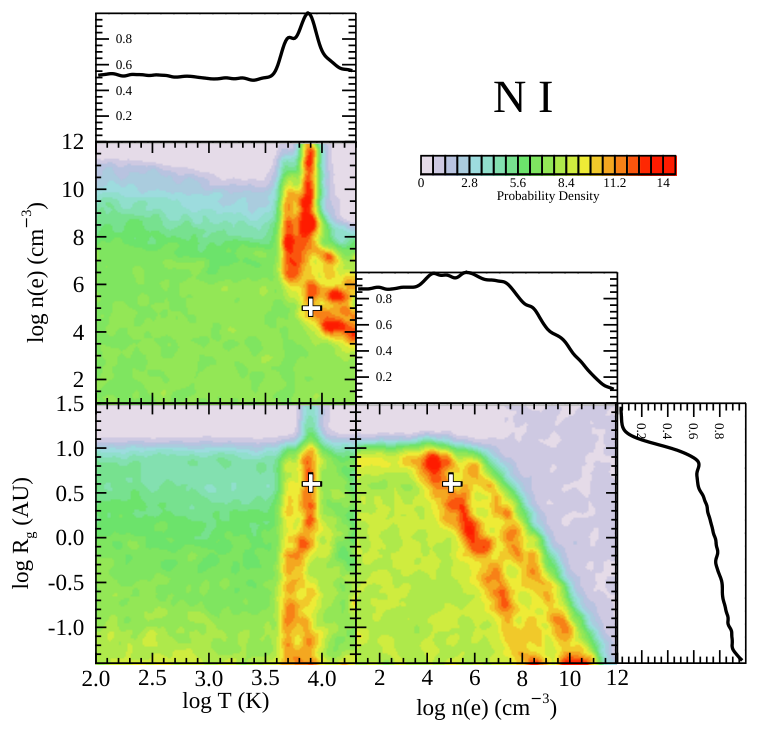
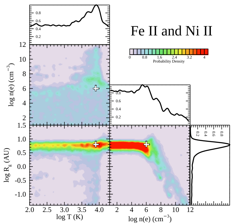
We have organized our investigation so that levels of Fe II and Ni II are analyzed jointly, but the levels of N I are treated separately. The rationale for this approach is that Fe and Ni are refractory elements that probably share a common location, whereas N is a volatile element that may be distributed differently within the circumstellar environment.
Figure 4 shows examples where the conditions exhibit favorable matches between the observed level populations and the predictions arising from the analysis discussed in Section VI.4. As will be clear from the results presented in the next section, these conditions are not the only ones that give satisfactory fits to the data.
VI.6 Outcomes
Figure 5 illustrates the coverages of high probabilities in the , and parameter space, which are depicted by the densities of successful trials in the MCMC runs. As expected, the outcomes for the most probable values of these parameters for N I and Fe II+Ni II sometimes differ from each other, yet there is still a broad range of choices where they overlap. This overlap suggests that at least some, or perhaps most, of the neutral and ionized constituents probably coexist within a common volume, rather than being separated from each other and situated in separate zones. We find that N I favors a temperature K (), and part of the outcomes for Fe II+Ni II are consistent with this result. Aside from temperature, the four metastable levels of N I constrain the possible combinations of the other conditions rather poorly. The results from Fe II+Ni II indicate rather well the distance to the star, AU (), and we can rule out values of that are significantly larger than . For these two ions, arbitrarily low values for the electron density and temperature are possible, which indicates that excitations due to optical pumping dominate over those from collisions by electrons. From our interpretation of our lower limit for the relative population of O I in the level that we derived in Section VI.5.2, we concluded that , which is consistent with the regions exhibiting high probabilities for the excitations of N I, Fe II, and Ni II.
VII Other Neutral Atoms and Their Ionization Equilibria
VII.1 Recombinations with Free Electrons
In previous sections, we discussed our findings on the circumstellar abundances of the neutral forms of two elements, O and N. These elements are plentiful, and the logarithm of the ratio of their abundances , which is not far from the solar abundance ratio 0.86 (Asplund et al. 2009).55 5 The difference from the solar abundance ratio decreases a bit when we consider that , as we will show later in Section X. For the neutral forms of species that should be predominantly ionized, a very different picture emerges, as we discuss below.
We now explore the implications for electron densities by comparing the column densities of elements in their neutral states to those of their singly-ionized states . The abundances of these two forms are influenced by an equilibrium between the starlight photoionization of the neutral atoms at a rate balanced against the sum of the radiative recombination (rr) and dielectronic recombination (dr) of the ions with free electrons with a combined rate constant at 8000 K.
We consider the formula for the ionization equilibrium for the element ,
| (21) |
where we have substituted observed column densities for the local densities and set
| (22) |
The dilution factor that we defined in Eq. 1 when . For AU, . This value is considerably larger than the interstellar UV and visible radiation field at our location in the Galaxy, which is described in terms of for a blackbody spectrum with K added to for K (Mathis et al. 1983) and even lower effective values of for very hot stars (Mezger et al. 1982). Hence, we can ignore the effects of the general radiation emitted by stars elsewhere. The upper limit for the integral is the wavelength of the ionization edge of the element in question ( if is expressed in eV), and is its ionization cross section. The stellar flux at the surface of the star is expressed in the form , which we defined in Section VI.1.1, and the factor in the equation converts from Å to cm. The lower integration limit of 920 Å corresponds to the cutoff in the stellar flux caused by high members of the Lyman series and Lyman limit continuum absorptions.
| Elem. | (6 AU) | aaDerived using , K, and the use of the fitting equation, Eq. 8 of Weingartner & Draine (2001b) for the element in question. See the text for details. | bbSolutions to Eq. 21. | ||||
|---|---|---|---|---|---|---|---|
| ) | ) | ) | ) | ||||
| (1) | (2) | (3) | (4) | (5) | (6) | (7) | (8) |
| C | 3.4e-03 | 6.7e-16 | 9.1e-13 | 1.9e-16 | 2.5e+12 | 2.3e+17ccThis value is not measured; instead, we had to estimate it by relating it to O and N and using a solar abundance ratio (Asplund et al. 2009). If this element is depleted relative to O and N, the value or upper limit for will be higher. | 4.0e+04ddThe abundance of C II is probably lower than the value given in Column 7. For this reason, the upper limit shown here is too low. See Section XI. |
| Na | 1.4e-02 | 4.5e-11 | 1.8e-13 | 3.3e-18 | 3.0e+10 | 6.5e+14ccThis value is not measured; instead, we had to estimate it by relating it to O and N and using a solar abundance ratio (Asplund et al. 2009). If this element is depleted relative to O and N, the value or upper limit for will be higher. | 3.6e+06 |
| Mg | 6.8e-02 | 2.1e-12 | 4.7e-12 | 9.0e-17 | 1.2e+12 | 1.4e+16ccThis value is not measured; instead, we had to estimate it by relating it to O and N and using a solar abundance ratio (Asplund et al. 2009). If this element is depleted relative to O and N, the value or upper limit for will be higher. | 1.3e+06 |
| Si | 4.7e+00 | 9.3e-13 | 1.7e-12 | 7.9e-17 | 3.3e+11 | 4.2e+15 | 2.2e+08 |
| P | 2.3e-01 | 3.0e-14 | 1.1e-12 | 4.3e+11 | 3.4e+13 | 2.5e+09 | |
| S | 1.6e-01 | 1.0e-14 | 4.7e-13 | 1.1e-16 | 5.5e+11 | 6.3e+15ccThis value is not measured; instead, we had to estimate it by relating it to O and N and using a solar abundance ratio (Asplund et al. 2009). If this element is depleted relative to O and N, the value or upper limit for will be higher. | 2.9e+07 |
| Cl | 2.5e-05 | 6.0e-16 | 1.2e-12 | 4.7e+13 | 4.4e+13 | 7.0e+07eeThis outcome is misleading for reasons outlined in Section VII.3. | |
| Ca | 1.1e+00 | 1.3e-11 | 6.2e-12 | 7.8e-18 | 2.8e+08 | 1.1e+11 | 4.4e+08 |
| Fe | 5.6e-01 | 4.0e-13 | 1.5e-12 | 5.7e-17 | 3.3e+11 | 1.3e+15 | 9.3e+07 |
| Zn | 2.0e-02 | 3.9e-11 | 4.5e+10 | 1.5e+13 | 1.5e+06 |
References. — used for computing : C (Verner et al. 1996); Si, Fe: NORAD-Atomic-Data website, https://norad.astronomy.osu.edu/; Mg: (Wang et al. 2010); S (Bautista et al. 1998); Ca: (Verner et al. 1996); Na, P, Cl, Zn: (Verner & Yakovlev 1995), Collisional ionization from electron impacts : (Voronov 1997), Recombination : C, Na, Mg: (Badnell 2006); Si: (Nahar 2000); P, Cl: (Landini & Monsignori Fossi 1991); S, Ca: (Shull & Van Steenberg 1982); Fe: (Nahar et al. 1997), Zn: (Mazzitelli & Mattioli 2002), Grain recombination for all elements where a value can be calculated: (Weingartner & Draine 2001b).
Numbers that are relevant for evaluating based on the ratios of neutrals to ions of various elements are listed in Table 3. Values of listed in Column (2) of the table are based on a radial distance from the star AU (i.e., , which was favored by the Fe II+Ni II metastable excitations; we recall that the stellar radius AU from Section VI.1.2). Equation 21 ignores the effects of collisional ionizations by electron impacts. At K, indicated by the N I excitations, we find the effects of such collisions to be very small compared to . For instance, we list the rate constants for such collisions in Column (3) of the table; for the largest value of indicated by the metastable excitations. At K, the dielectronic recombinations are substantial for the elements Mg, Ca, and Zn, and the inferred values for change rapidly as a function of temperature for Mg and Ca. The quantity in Column (5) will be discussed in Section VII.2.
We start by comparing the abundances of neutral and singly-ionized carbon. For the former, we stated in Table 2 a measurement66 6 Our determination is considerably lower than that of Lecavelier Des Etangs et al. (1997a) of based on a GHRS G160M spectrum taken at a different time – see Table 1). , but we conclude that the origin of this C I absorption is interstellar based on two arguments: first, it has a velocity of with respect to the other strongest circumstellar features (see Section IV), and second, we see no evidence of absorption out of either of the two excited fine-structure levels. In a very dense and hot gas, the populations of all three fine-structure levels should be in proportion to their degeneracies. Thus, in our attempt to identify C I associated with the circumstellar gas, it is best to try to measure features out of the level at , which has a degeneracy equal to 5 (compared to 3 and 1 for the other two levels). After considering relative signal-to-noise ratios and the groupings of lines within the different multiplets, we chose to use the two lines listed in Table 7 for this level. The absorptions cannot be seen in the spectrum, so we derived an upper limit equal to using the method described in Section III.2. We then multiply this upper limit by 9/5 to account for C I in the other two levels to arrive at a total upper limit (C I).
For C II, we must make a preliminary estimate for its column density because our determination from a semiforbidden transition is quite high (the allowed transition at 1334.5 Å is very badly saturated and not useful). If we assume that the ratio of C to O or N in the circumstellar gas is identical to the solar ratio (Asplund et al. 2009), we arrive at an approximate value . At a radial distance from the star AU, our determination of in Eq. 22 gives a value when we use the ionization cross sections provided by Verner et al. (1996). For carbon ions, at K (Badnell 2006). An application of Eq. 21 to our upper limit for (C I) yields . This limit is below the example for that we chose to represent for the excitation of N I in Fig. 4, but setting equal to the limit does not significantly degrade the match with the data and is consistent with our lower limit that we derived from the population of the O I metastable level in Section VI.5.2.
Our calculation for only considered direct photoionization by the flux from the star. From the presence of N II we know that ionized hydrogen must be abundant. We will argue later (Section XII.4) that H must be ionized by photons that are far more energetic than this atom’s ionization potential. When this happens, the electrons that are released can produce secondary ionizations of other elements, including C. Because we did not include secondary ionizations in our calculations, it is possible that the outcome of our calculation of the upper limit for is too low because we underestimated the true total value of .
In principle, another route for ionizing the carbon atoms is through the charge exchange reaction . However, this process is quantitatively unimportant since even for a very large proton density, say perhaps , the effect of this reaction is 7 orders of magnitude weaker than the photoionization rate because its rate constant is only at K (Butler & Dalgarno 1980). (In contrast to carbon, we find that charge exchange reactions that involve chlorine are important, as we will show in Section VII.3).
We summarize in Column (8) of Table 3 the values of that we derived for C and various other elements using Eq. 21. For Fe I the combined degeneracies of the other four fine-structure levels of this atom compared to of the lowest level could mean that our upper limit for all of the Fe I should be increased by a factor of 25/9 to if the excitation temperature is large. Our limit for (Fe I) is considerably lower than the amount that appears in the spectrum of Pic (Vidal-Madjar et al. 2017 ; Kiefer et al. 2019). The column density for Fe II includes all of the levels that we observed plus reasonable estimates for the populations of intermediate levels that we did not observe (to be discussed later in Section IX).
While most of the upper limits for are consistent with our derivation based on C, there are two major inconsistencies with the C result. The most prominent disagreement is the outcome of a lower limit for derived from chlorine. In Section VII.3 we will explain why we can disregard this result. The outcomes for Na and Zn are substantially higher than that for C, which probably indicates that the actual (C II) is lower than our assumed value. We will discuss the possibility that neutral carbon atoms might be expelled by an outward radiation pressure arising from the stellar flux in Section XI. That discussion will rely on conclusions derived here on the ionization and recombination of carbon atoms and ions and how these processes should affect any outward migration of the atoms.
VII.2 Interactions with Dust Grains
Up to now, we have not considered recombinations of the ions with electrons on the surfaces of dust grains (Snow 1975 ; Weingartner & Draine 2001b). The efficiency of this process depends on the local density of grains and their charge. Our discussion will proceed within the framework of the dust-to-gas ratio being identical to that of the general ISM. However, we note that in reality it may be lower in the circumstellar atomic gas region that we sampled – at least for grains in the size range that is important for reddening. The color excess E() for 51 Oph has been reported to be 0.04 by Malfait et al. (1998) and by Manoj et al. (2006). Using our measured column densities of N I and O I and assuming that their depletions are consistent with a moderate density ISM (i.e., in the characterization of Jenkins (2009)), we would expect to find that , as we will explain in more detail in Section X. This value is greater than what we would have expected from the general result of Diplas & Savage (1994) for the ISM, where , which would yield for the two determinations of E(). This disparity, which is made even worse by the presence of ionized hydrogen, may indicate that some fraction of the grains have been driven out of the circumstellar atomic gas by an outward radiation pressure. Nevertheless, in the discussion that follows, we will frame our arguments within a perspective that the relative proportion of grains in the gas and their size distribution are the same as in the general ISM.
The charge of the grains is regulated by a balance between the loss of electrons due to photoelectric emission, which is governed by the local radiation density, and the capture of free electrons, which depends on (Weingartner & Draine 2001a). In a formalism developed by Weingartner & Draine (2001b) for the neutralization of ions by grains in the general ISM, a rate coefficient is normalized to the local hydrogen density and depends on the parameter
| (23) |
and , where is the radiation density relative to that in the ISM as defined by Mathis et al. (1983). The flux of 51 Oph at its surface corresponds to for photons with Å. In the panel that shows vs. for N I in Figure 5, the right-hand edge of the diagonal, red-colored region showing the most probable combinations corresponds to , where is expressed in cm-3 and in AU. Here, we have chosen the highest set of values for to explore the most favorable condition for promoting the neutralization of ions by their interactions with grains. Because , we obtain the simple outcome for the lowest value (i.e., one that is the most conservative from the standpoint of giving the highest values for ).
We do not have a firm number for a representative value of , but if we assume that the column density (from our measurements of N I and O I) and the thickness of the zone is no smaller than about , we obtain the estimate . When we combine this limit with our condition , we obtain an outcome for the electron fraction , which equals if AU. As long as is not less than , we can declare that recombinations onto grains are less important than recombinations with free electrons. (Even if is smaller than this example, one should recall that from the discussion in Section VI.5.2.) The results shown in Table 3 indicate that for all of the elements, , so we can ignore the influence of grains in the ionization equilibrium.
VII.3 An Interpretation of the Large Abundance of Neutral Chlorine
The ionization balance for chlorine is vastly different from the examples that applied to the other elements listed in Table 3. We find a very strong presence of Cl I ( for the sum of the two fine-structure levels that we observed), but we were unable to detect an absorption feature out of the singly-ionized form of Cl. The outcome shown in the table indicates that the lower limit for is strongly inconsistent with the values or limits derived for C, Na, Mg, S, and Zn. The only ways to reduce the inferred value of are either to lower the temperature to well below K (thus increasing ) or to consider that AU. The probabilities indicated in Figure 5 reveal that the former possibility is disfavored by the N I excitations and the latter is ruled out by the Fe II+Ni II excitations.
We now reach a point where we must consider alternate means for neutralizing Cl. One of them might be the reaction followed by the dissociative recombination with electrons to form neutral hydrogen and chlorine (Jura 1974 ; Smith et al. 1980). The possible importance of this channel is supported by observations of the ISM that show a strong correlation between (Cl I) and and evidence that in a number of cases (Moomey et al. 2011). However, we regard this process as unimportant for the material surrounding 51 Oph, because Roberge et al. (2002) found that in the and states in the ground vibrational level, which is far lower than typical amounts of that were found in ISM sight lines that showed enhancements of Cl I.
Still another pathway for neutralizing Cl ions is through charge exchange with neutral hydrogen, . The reaction is endothermic, but not strongly so because the first-ionization potential of Cl is 12.97 eV, which is only slightly below that of hydrogen. The rate constant for this reaction is
| (24) |
and the reverse reaction rate is
| (25) |
(Pradhan & Dalgarno 1994). At K, and . We now examine the equilibrium of the two chlorine ionization states that takes into account these reactions, along with recombinations with free electrons and starlight photoionizations (at rates specified in Table 3):
| (26) |
When solving this equation for we find that the term is insignificant and obtain the numerical result:
| (27) |
Because our observation indicates that , the above expression gives a lower limit:
| (28) |
This outcome demonstrates that even with the large electron densities indicated by the metastable level populations, the neutral fraction of hydrogen is significant, which is a conclusion that is consistent with our observed abundances of N I and O I. The fact that we could not obtain a column density for N II and compare it with N I means that our knowledge on the neutral versus ionized hydrogen abundances is limited to our finding expressed here and the less definitive estimate at AU derived in Section VII.2.
VIII The Allowed Transitions of O I to the Level
Figure 6 shows the spectrum of 51 Oph over a wavelength interval that covers the very strong features from three fine-structure levels of the ground electronic state of O I. The levels and have excitation energies equal to 158 and , respectively, above the state. The absorption features from the excited levels of O I have cores that do not reach zero intensity, unlike the absorptions from the ground states of both O I and Si II. The excited fine-structure level of Si II also does not reach zero intensity, but it is closer to zero than the features of excited O I.

While one might envision that the profiles do not reach zero intensity because the absorbing medium does not completely cover the disk of star seen in projection, we propose that a more likely explanation is that some of the flux from the star is resonantly scattered by oxygen atoms in the far side of the circumstellar disk.77 7 We can dismiss the notion that the emission could be caused by telluric O I emission, because if this were so, we would find the same effect in the unexcited O I line at 1302 Å. If some of this emission were able to bypass the foreground absorption in the near side of the disk because it was somewhat displaced in projection, it would create excess flux contributions which fill in positive intensities superposed on the two saturated line cores. Portions of the emitting gas that subtend less than should be admitted through the entrance aperture of the spectrograph, where (Arenou et al. 2018 ; Luri et al. 2018) is the distance of the star from us in units of 100 pc. This emission effect is not seen in the feature from the unexcited state because it is blocked by foreground O I in the interstellar medium, whereas the interstellar absorption from the two excited levels is extremely weak or nonexistent.
A plausible configuration for our being able to view the emission from resonant scattering is depicted in Figure 7. If the disk has a wedge-shaped cross section and the vertex falls short of the star, both sides can be illuminated by radiation from the star. We know from the nondetection of CO discussed in Section V that we are not viewing the disk edge on. If the tilt of the disk with respect to the observer is sufficient, light scattered by atoms in the rear portion could bypass gas in the foreground part that would otherwise absorb it. Under the right conditions, other geometries that could also create conditions for this phenomenon might include circumstellar rings or warped disks.
Figure 8 shows the spectrum in the vicinity of the excited lines after the intensities have been normalized to the stellar continuum (black trace). To estimate the strengths and shapes of the emission profiles, we must first estimate what the absorption would look like in the absence of emission. To recreate this absorption, we used our value for (O I) in the level that we derived from the weak intersystem line at 1355.598 Å, as listed in Table 2, and assumed that each fine-structure level was populated in proportion to its degeneracy, which is approximately valid if the medium is dense and has an excitation temperature is of order 8000 K. Next, we used the velocity parameters for our neutral gas absorptions that we described in Section IV to construct the expected profiles. The red trace in the plot shows the absorption profiles that should arise from this model. The effect of smoothing by the STIS line spread function is very small for such wide absorption features, but it has been included. As a check on the validity of this reconstruction, we require that the two profiles do not extend beyond the velocity span of the absorption from the unexcited level, which should be stronger because it has a higher degeneracy than either of the two excited levels. The green traces show the absorption by the unexcited level superposed on the two excited level absorptions. In both cases, the red traces fall inside or on the green ones.
The blue traces in the figure show the differences between the observed intensities and our reconstruction of what the absorption features should look like in the absence of any emission. The broadening of the emission should arise from the Keplerian motion of gas around the star, and the increased levels of intensity away from the line center are probably created by limb brightening along the tangent points. Both of the emission profiles reach zero intensity at about 20 away from the line center, and this velocity offset is consistent with the expected Keplerian velocity at AU from the star, where the star has a mass equal to (Jamialahmadi et al. 2015). The intensity dip seen on the right-hand side of the profile is caused by telluric O I absorption, which we predict to occur at a heliocentric velocity of +9.9 at the time the observation was carried out (or +26.9 for the scale shown in Fig. 8). If the gas were optically thin, we would expect the emission intensity to be three times as strong as that from the state, but here it appears to be only about twice as strong. High optical depths would tend to equalize the two intensities, but at some expense to the limb-brightening effect.
We touch briefly on the possibility that some of the emission might arise from Bowen fluorescence (Bowen 1947) produced by optical pumping by L irradiation to the levels in the states, which then decay to produce radiation at 8446Å. Eventually, there is a cascade to the state that produces 1304 and 1306Å photons as it decays to the ground fine-structure levels. Broad H emission arising from a shock in an accretion flow has been observed for 51 Oph (Manoj et al. 2006 ; Mendigutía et al. 2011). If the medium is optically thin, the predicted value of is 7500 (Strittmatter et al. 1977), but it can be lower if the emitting region is optically thick. For the feature, the average strength of the emission over the 40 span centered on the systemic velocity () is 0.10 times the continuum intensity over the same interval. We compute that the prediction for the fluorescence would result in about one order of magnitude less flux than what we observe, but a higher intensity could result if the region is optically thick or there is a sufficient flux of L photons from the star.
IX The Pattern of Element Abundances

Figure 9 is a representation of vs. excitation energy for the key elements covered in this study. For many of the elements, there are levels whose absorptions we did not observe and yet would be expected to be populated. For the elements Cr, Mn, Fe, Ni, and Cu, we estimated the locations for the unobserved levels in this diagram by placing them on a straight-line best fit to the measured levels. Unseen levels that were considered to have populations worthy of note were those that had excitation energies below and that did not have electric dipole or intercombination lines to lower levels that would cause rapid radiative decays. The elements N, O, Si, and Zn did not have any such unseen levels. For the elements P, Ti, and Co, the observations were so incomplete that we had to adopt a representative slope, and we chose one that was equal to the mean of the Fe II and Ni II fits. The situation for O is a special one; aside from the fine-structure levels, the only noteworthy excited level is the one at that we know has an appreciable column density, but for which we could derive only a lower limit to its value. The circle symbol in the diagram corresponds to our expectation for and K.
| Log Total | Fraction | Excitation | |
|---|---|---|---|
| Element | Column Density | Observed | Temperature (K) |
| (1) | (2) | (3) | (4) |
| N | 16.60 | 1.00 | 5180 |
| O | 17.63 | 0.98aaWe could measure only the ground level, but the other two fine-structure levels should be populated in proportion to their degeneracies. While we observed an absorption out of the metastable level at an excitation of we could only obtain a lower limit for its column density. | |
| Si | 15.62 | 1.00 | 890bbFine-structure levels only. |
| P | 13.61 | 0.85 | 450bbFine-structure levels only. |
| Ti | 12.24 | 0.05 | |
| Cr | 13.49 | 0.61 | 11,990 |
| Mn | 13.27 | 0.78 | 9120 |
| Fe | 15.15 | 0.94 | 3090bbFine-structure levels only., 11,840ccMetastable levels only. |
| Co | 13.28 | 0.27 | |
| Ni | 13.81 | 0.99 | 10,210 |
| Cu | 12.49 | 0.88 | 9700 |
| Zn | 13.61 | 1.00 |
We may be mildly understating the abundances of nitrogen and oxygen, as some fraction of these elements may be singly ionized, i.e., a condition similar to that of hydrogen. We know from the FUSE observations discussed in Section VI.5.2 that this is the case for nitrogen, but we are not able to quantify the relative ionization. Later, in Table 5 within Section X, we will show our estimates for the ratios of ions to neutrals for these elements. The other elements probably have no appreciable concentrations in their doubly ionized form, but we have no firm evidence that this is so.
Table 4 shows some outcomes of our measurements of the elements. Column (2) lists the sum of observed and unobserved column densities, while Column (3) shows the fraction of this combined column density that was actually observed, which can be used as a measure of the reliability of the total column density. The excitation temperatures given in Column (4) are derived from the negative inverses of the slopes of the level populations shown in Fig. 9. From the conclusions that we derived in Section VI.6, it should be clear that these excitation temperatures should not be regarded as actual physical temperatures. We list these temperatures only for the purpose of empirical comparisons with results for the circumstellar populations around other stars. In particular, we caution against using the populations of the fine-structure levels of Si II and P II as an alternate means of determining and because the uncertainties in the column densities are large enough to allow their excitation temperatures to be equal to the kinetic temperature. For instance, the critical density for the excitation of the Si II levels is as low as (Silva & Viegas 2002, Fig. 8).
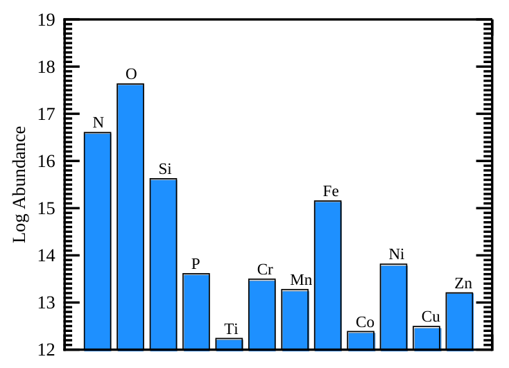
.
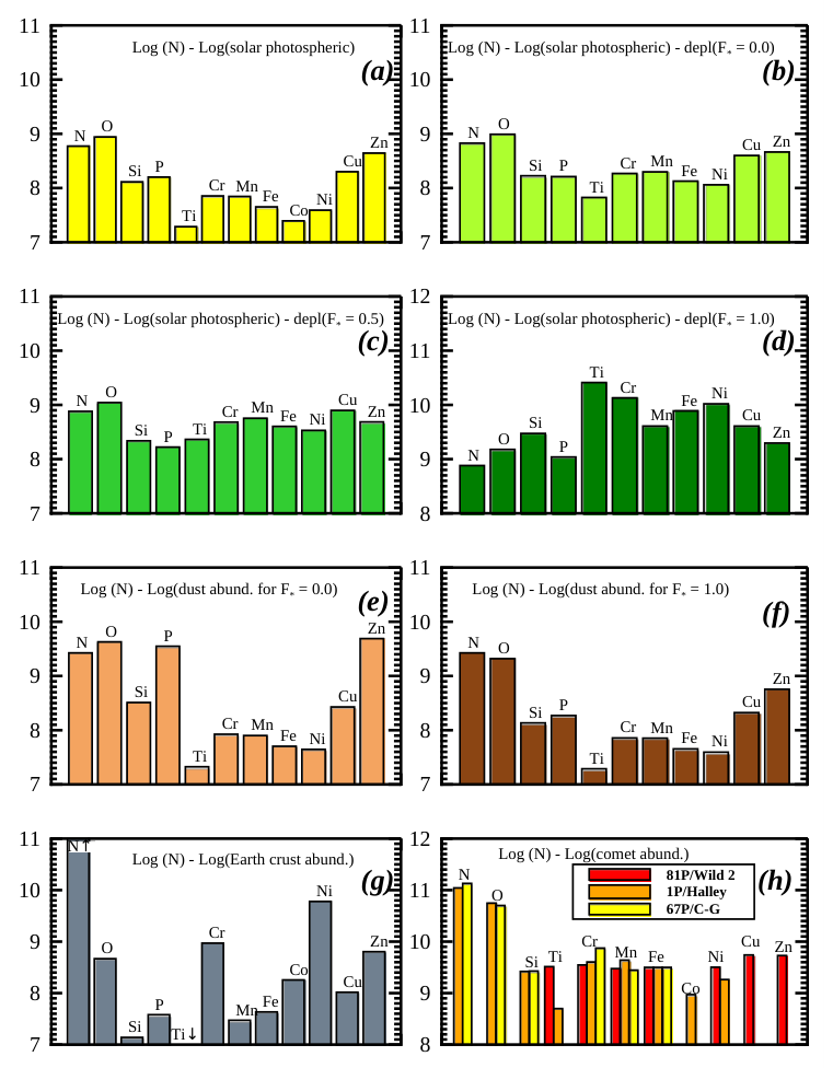
We present the pattern of the total logarithmic column densities in Figure 10. Our next step will be to explore some possible interpretations of these abundances. Figure 11 presents a number of choices. In panel of this figure, we show a representation of our total logarithmic column densities listed in Table 4 after subtracting the logarithm of the solar photospheric abundances (on a scale H = 12) (Asplund et al. 2009) to test the proposition that the gas that we measured is dominated either by mass loss from the star or by interstellar material that has virtually no depletions of atoms onto dust grains. The lack of uniformity in the bar heights indicates that this is not a favorable interpretation. Next, we apply the same test for gas that has a composition that is similar to that of the general ISM with three possible choices for the severity of atomic depletions. These choices are represented by the expected depletions for the parameter (Jenkins 2009), which ranged from values of 0.0 (i.e., very light depletions) in Panel , 0.5 (moderate depletions) in Panel , and 1.0 (heavy depletions) in Panel .88 8 The depletions of P and Zn have been modified from the original description by Jenkins (2009) to account for the revised -values for transitions of P by Brown et al. (2018) and Zn by Kisielius et al. (2015) that replace earlier ones reported by Morton (2003). The moderate depletions () seem to show the best uniformity in the bar heights.
The lower four panels of Fig. 11 test the proposition that the original gas that has condensed out of the ISM to form the circumstellar disk has been expelled and been replaced by atomic constituents arising from different possible forms of solid material that have been converted into gaseous form by collisions or ablation. Recall that from our finding stated in Section V about the absence of CO features in our spectrum, we concluded that we must be sampling gas at some distance from the midplane of the disk. This gas might have been subject to erosion by photoevaporation or a stellar wind and replaced by elements arising from destructive processes for solids in the midplane. Panels and represent our abundances after subtracting the pattern of abundances of ISM dust for and 1, respectively. The bar heights are quite uneven in these panels. The same kind of presentation is presented for Earth’s crust abundances (Anderson 1989 p. 150), which could stand for material ejected from the outer portions of chemically differentiated planets by collisions (Panel ). We have also tested the pattern that could emerge from the destruction of objects that have chemical makeups similar to those of CI chondritic meteorites (Lodders 2003). However, except for volatile elements, the abundances in such primitive meteorites closely follow the solar photospheric ones, so we would simply be duplicating what we see in Panel , except for the elements N and O. Finally, in Panel we investigate the relative differences between our abundances and those found for three different determinations of some relative abundances for cometary dust: (1) dust from Comet 81P/Wild 2 collected in the aerogel on the Stardust mission (Flynn et al. 2006), (2) material observed with the impact-ionization time-of-flight mass spectrometer in the PUMA-1 experiment on the VEGA-1 spacecraft, which encountered Comet 1P/Halley (Jessberger et al. 1988), and (3) the sampling of particles from Comet 67P/Churyumov-Gerasimenko by the COmetary Secondary Ion Mass Analyzer (COSIMA) on the Rosetta mission (Bardyn et al. 2017). Comets 81P/Wild 2 and 67P/Churyumov-Gerasimenko are Jupiter-family comets (with a low orbital inclination and perturbed by Jupiter into a short period), and 1P/Halley is a long-period comet with a high inclination.
From the choices that we presented in Fig. 11, we conclude that ISM-type gas that has undergone moderate levels of depletion gives a satisfactory match to the abundance pattern that we observed. Over a limited range of refractory elements that were reported, the results for 81P/Wild 2 and 67P/Churyumov-Gerasimenko also seem to show a reasonably good uniformity of bar heights, but for Halley and 67P our abundances of N and O seem too large. The ISM dust solids and the Earth’s crust material outcomes show significantly uneven bar heights in their respective panels.
X Estimates for the Column Densities of H I and H II
Even though we cannot directly observe hydrogen in its neutral or ionized forms, we can make use of the good match between the abundance pattern of different elements to that of a mildly depleted gas-phase ISM to propose that the volatile elements N and O can be used as proxies for H after correcting for abundance differences. Again referring to the ISM, we conclude that the circumstellar N and O should be depleted by about 0.1 dex below their protosolar abundances. From the evidence presented in Section VI.6, we adopt the viewpoint that the neutral hydrogen atoms and protons are distributed in a common volume, rather than being in separate locations.
The ionization fractions of N and O are coupled to that of H by charge exchange reactions with large rate constants. As we will discuss in Section XII, the ionization levels for all three elements must be maintained by photoionizations caused by energetic radiation in excess of the flux from the star at wavelengths below the Lyman limit (and perhaps supplemented to some extent by cosmic-ray ionization).
In order to have a good understanding about the strength of the coupling of the relative ionizations of nitrogen and oxygen to that of hydrogen, we must know the volume densities and . Our constraints on these quantities cover some broad ranges in values. From the metastable excitations and the ratios of some neutral atoms to their ionized counterparts, we feel that it is reasonable to adopt . For neutral hydrogen, we described in Section VII.3 how the abundance of neutral chlorine compared to an upper limit to its ionized form led to an expression given Eq. 28, but we must remember that the specified value for is a lower limit. We have no direct way to constrain how far above this limit the density could go, other than to argue that if it were to reach , our determination of the column density (which we will derive shortly) divided by would shrink to a thickness (i.e., 0.6 AU), which we can deem to be a reasonable lower limit.
To determine the ionization balance of nitrogen, we can use the charge exchange rate constants and derived by Lin et al. (2005) for K. The recombination coefficient for nitrogen is at K (Shull & Van Steenberg 1982 ; Nussbaumer & Storey 1983). The value of is about ten times the value of after one considers additional secondary ionization processes for both elements (Jenkins 2013). Because the region is optically thick to Lyman limit photons, we adopt a recombination rate to levels and higher at K. We now can substitute N for Cl in Eq. 26 and solve for to obtain the estimates listed in Table 5 and compare them to their hydrogen counterparts , also listed in the table. We now define an ionization correction factor
| (29) |
| min[] | min[] | max[] | max[] | |
|---|---|---|---|---|
| Quantity | min[] | max[] | min[] | max[] |
| n(e) (cm^-3) | 10^5 | 10^5 | 3×10^6 | 3×10^6 |
| n(H^0) (cm^-3) | 3.5×10^5 | 10^8 | 8.4×10^6 | 10^8 |
| n(H^+)/n(H^0) | 0.285 | 10^-3 | 0.36 | 0.03 |
| n(N^+)/n(N^0) | 0.63 | 5.5×10^-4 | 0.82 | 0.0315 |
| Y(N) | 0.10 | 0.00 | 0.13 | 0.00 |
| n(O^+)/n(O^0) | 0.25 | 9×10^-4 | 0.31 | 3×10^-2 |
| Y(O) | -0.01 | 0.00 | -0.02 | 0.00 |
From our observation of N I, we evaluate our estimate for using the relation
| (30) |
where we use our determination of listed in Table 4, and the protosolar abundance (Asplund et al. 2009). The term 0.1 in the equation is a correction that applies to our estimate of the depletion of N. The stated value given in Eq. 30 is for , which recognizes that the FUSE spectrum exhibited strong absorptions of the N II multiplet near 1085 Å, as we had indicated earlier in Section VI.5.2. The uncertainty for the result includes both the range in possible values and the uncertainty in the measurement of added in quadrature.
For oxygen, we may repeat the calculation that we carried out for nitrogen, again adopting rates at K. Here, we make use of Draine’s (2011, p. 155) characterization of the charge exchange reaction rates calculated by Stancil et al. (1999) between O+ and the three fine-structure levels of O0, yielding for the three levels and , for the levels of O0. As with nitrogen, of . For oxygen, (Shull & Van Steenberg 1982 ; Nussbaumer & Storey 1983).
An application of Eq. 30 for O with and again assuming a depletion correction of 0.1 dex yields the result . The uncertainty for this result is dominated by the measurement uncertainty for ; possible values of given in the last row of Table 5 are close to zero and small compared to the uncertainty in . Because the determination of the column density of H I based on O is substantially more precise than that for N, we adopt this value but note that the outcome for N is consistent with that for O within our uncertainties of and .
If we treat the expression for in Eq. 28 as an equality, rather than a limit, and then evaluate a characteristic length scale we obtain the result and 190 AU for and , respectively. Because both of these values for are larger than our representative value AU, the inequality in Eq. 28 must apply to some extent.
Again we can use Eq. 28 to arrive at a column density for ionized hydrogen and 20.56 for and , respectively.
XI A Deficiency of Carbon
XI.1 Abundance Estimate
Unlike the preferred ionization stages of N and O, whose neutral forms we could measure using weak transitions to obtain column densities, the dominant phase of C (C II) exhibits only two transitions: (1) an allowed transition at 1334.5 Å that is far too strong to be useful for measuring (C II) and (2) an intersystem line at 2325.4 Å that is so weak that it provides an upper limit for (C II) that is far too high to be of any use. To gain an understanding about the abundance of carbon, we must direct our attention to the neutral form of this element and attempt to relate it to the total abundance of carbon in the gas phase.
As we discussed in Section VII.1, our inability to detect an absorption from one of the excited fine-structure levels of C I sets a limit on the abundance of neutral carbon . This limit for the amount of C I is substantially lower than the findings by Roberge et al. (2000) that for Pic and for 49 Cet (Roberge et al. 2014). A comparison of the 49 Cet result against ours is especially noteworthy, since they found considerably more C I than our upper limit, yet their sum of results for in the and levels equaled compared to our result for the same sum of . (The A1V spectral type of 49 Cet is only slightly later than that of 51 Oph.) From this disparity in the observations of the neutral forms of C and O, we might conclude that and/or for the gas around 49 Cet is larger than what we found for 51 Oph, thus favoring a shift in the ionization equilibrium toward a higher neutral fraction for carbon, or alternatively, the ratio of the C to O abundance in the gas surrounding 49 Cet is larger than that associated with 51 Oph.
A contributing factor that drives a deficiency of C I is the high value of at AU, but our conclusion given in Table 3 that relied on the abundance of carbon (mostly ionized) being in accord with an expectation based on solar abundance ratios relative to the neutral forms of oxygen and nitrogen. To make the calculation of consistent with our findings for the ionization equilibrium outcomes for Na and Zn listed in Table 3, and also put us closer to the middle of the realm of that we found from the metastable level populations, we would need to reduce our assumed abundance of C by at least a factor of 40.
XI.2 Expulsion by Radiation Pressure?
We now explore one possibility for depleting C in the gas. A common theme in the study of circumstellar atomic gases is the consideration that the star’s outward radiation pressure can weaken or overcome the gravitation attraction for atoms (and some dust grains) in orbit (Beust et al. 1989 ; Lagrange et al. 1998 ; Olofsson et al. 2001 ; Liseau 2003 ; Brandeker et al. 2004 ; Fernández et al. 2006 ; Xie et al. 2013). The parameter describes the ratio of these two forces, , which is independent of the distance from the star since they both scale in proportion to . For any transition (which we identify with a subscript ) with an -value equal to , the exposure of an atom to a local flux vector will absorb photons at a rate99 9 Unlike our previous formulations for the effects of starlight, we do not consider a dilution factor for the radiation at some distance from the star because the projections of the momentum transfer events along the radial direction are the relevant quantities in the equation, rather than the total photon interaction rates of the atoms.
| (31) |
where and are the charge and mass of the electron, and is the flux of photons per unit frequency for the transition being considered. The factor represents the probability that the atom is in the appropriate fine-structure level for the transition at the wavelength . Each absorption imparts a radial momentum impulse . Hence, we find that if the absorption lines for all transitions have low central optical depths (i.e., there is no self-shielding of the radiation from the star), we obtain for neutral carbon
| (32) |
where is the effective stellar radius (see Section VI.1.2), is the mass of the star (Jamialahmadi et al. 2015), and is the mass of the carbon atom (12 amu). We calculate that for 51 Oph when we evaluate the sum in Eq. 32 over all C I transitions listed in the compilation of Morton (2003). This value is 20,000 times the value 0.033 computed by Fernández et al. (2006) for Pic, largely due to the fact that UV flux from Pic with K is about 4 orders of magnitude weaker than that of 51 Oph at the wavelengths of the strongest C I transitions. A similar calculation by Lagrange et al. (1998) for Pic gave that ranged between 0.011 and 0.095, depending on the amount of self-shielding in the lines.
We now argue that even though is quite large (considerably in excess of 0.5, which is the threshold for becoming unbound), the atoms are unlikely to migrate outward. At 6 AU from the star, each atom experiences an average rate of absorption , while concurrently it is exposed to an ionization rate . After a carbon ion is neutralized, we expect that over the survival time of its neutral form, , the radiation pressure accelerates it in a radial direction and increases its kinetic energy by , where
| (33) |
(Recall from our discussion in Section VII.1 that the ionization of by charge exchange with protons is negligible compared to , but could be enhanced by secondary ionizations arising from energetic electrons produced by the ionization of H.) We note that because is proportional to (for ), the value of does not change with . The kinetic energy of the Keplerian motion
| (34) |
receives a relative boost
| (35) |
Numerically, we find that Eq. 35 yields a result for the fractional increase in equal to for AU. After receiving this small boost in kinetic energy, the neutral atom becomes ionized and remains in that state for a time interval that averages for (or one-tenth that time for ). The value that we assign for at K still applies, because the suprathermal arising from Eq. 33 is small compared to the thermal velocities. During that time interval, the strong coupling of the carbon ions to other ions via Coulomb collisions (and possibly an embedded magnetic field) will force them to surrender their enhanced velocity and merge with the flow. Details on the physics of this ionic braking process are given by Beust et al. (1989), Fernández et al. (2006) and Xie et al. (2013).
We now conclude that even though is large, there presently is little chance that the carbon atoms can migrate outward. Instead, they must blend in with the circulating river of ions in Keplerian orbits. At some much earlier time when the protostar was emitting strong radiation but not at energies capable of ionizing the medium, the carbon may have had a chance to escape. However, it seems puzzling that carbon in an atomic form is currently not being replenished by dissociating CO molecules at the boundary of the thin molecular disk. Also, the present-day deficiency of carbon may present a challenge to the notion that the gas is composed of byproducts from cometary destruction that we discussed at the end of Section IX. We note, however, that Roberge et al. (2002) found a lack of C compared to expectations from N and Fe for transient gas components infalling toward 51 Oph.
It is likely that the elements O and N can maintain a neutral state much longer than the dwell time for neutral C. However, we expect that their values are considerably lower than that of C0 because they have fewer transitions in the UV and these transitions are strongly saturated. (In computations of , it is better to use the actual line equivalent widths that were or would have been observed instead of those that apply to unsaturated lines, as was done for Eqs. 31 and 32).
XII Discussion and Summary
The spectrum of 51 Oph has a rich assortment of absorption features arising from atomic constituents in a region within about 10 AU of the star. We have made use of 304 different transitions from 16 different elements for which we could measure the column densities for a total of 98 different atomic levels, most of which are highly excited and can come only from the environment near the star and not the foreground ISM. For 9 additional species, we searched for 14 strong transitions but could only determine upper (or lower) limits for the column densities. After determining column densities from the spectral features, we were able to derive a number of conclusions on the nature of the gas in the vicinity of the star. These conclusions are summarized very briefly in Table 6.
| Property | Value | Method |
|---|---|---|
| n(e) | N I, Fe II, and Ni II metastable populations (Sections VI.5.3 and VI.6) | |
| Na I, Zn I ionization equilibria (Section VII.1) | ||
| n(H) | Cl I and Cl II charge exchange (Section VII.3) | |
| N(H I) | (O I) and (N I) (Section IX) combined with | |
| charge exchange and protosolar abundances (Section X) | ||
| N(H II) | (Section X) | |
| T | 8000 K | N I, Fe II, and Ni II metastable populations (Sections VI.5.3 and VI.6) |
| Element | A pattern consistent with | Contents of Section IX |
| Abundances | a mildly depleted ISM | and the best matches in Fig. 11 |
| or Jupiter-class comet dust | ||
| Representative distance | 6 AU | Fe II, Ni II metastable populations (Sections VI.5.3 and VI.6) |
| from the star R_g |
XII.1 Disk Orientation
In Section V we noted that the contrast between the absence of both CO and H2 absorptions in the UV spectrum of 51 Oph and the detection of CO in emission in the far infrared indicates that we must be sampling regions away from the central plane of the disk where the molecules are shielded and thus protected from dissociating radiation that can reduce the molecular fraction to a very low value. Thus, while the disk may be seem to be nearly edge on from our viewpoint, it is not exactly so. This slight misalignment could explain why we can view resonantly scattered starlight in the bottoms of the saturated absorption features of O I. Our results, when combined with a future, accurate determination of the disk inclination,1010 10 Determinations that we could find in the literature: (Thi et al. 2005), (Berthoud et al. 2007), and 80°(no uncertainty specified) (Thi et al. 2013). would help to constrain the scale height of the molecular material.
XII.2 Ionization State
Our sight line to 51 Oph consists of significant portions of both neutral and ionized hydrogen, which we could not observe directly, but instead could be sensed from the abundances of neutral and ionized nitrogen. Further support for the existence of both kinds of gas arises from the metastable level populations of N I that indicate large electron densities, along with the surprisingly strong presence of neutral chlorine that must arise from charge exchange reactions with neutral hydrogen.
XII.3 Excitation Mechanisms
Using atomic data that we could find in the literature for N I, Fe II, and Ni II, we can interpret our measurements of their excited metastable levels in a manner that offered important clues on the condition and location of the gas. The populations of these levels are maintained by a combination of optical pumping by starlight and collisions with electrons. The findings for the strengths of these two effects are somewhat degenerate with each other, but our MCMC analysis allowed us to focus on a restricted range for their possible combinations. For the conditions that we found, collisions with neutral hydrogen atoms should have a minimal effect on such excitations.
We acknowledge that we have oversimplified our descriptions of the metastable level excitations in terms of a gas at a particular distance from the star which has a uniform electron density and temperature. Nevertheless, future interpretations that invoke interpretations of more extended gas structures having variable conditions should still be able to make use of our simplified conclusions on what we can regard as density-weighted values for these parameters as a starting point. Such modeling may also include a picture where the N I is located in a different region than that which highlights the presence of Fe II and Ni II. Some support for a difference in the distributions of ions and neutrals arises from the fact that the ions show both a principal, narrow-velocity component (Component 1 described in Section IV) and a broader, weaker, slightly displaced one (Component 2), while the neutrals show only Component 1 with no evidence for Component 2, except perhaps for a one-percent contribution that may be evident in a very strong line of O I.
XII.4 Electron Density
An important finding of our investigation on the metastable level populations is that the electron densities fall somewhere in the range . The neutral to ionized fractions of Na and Zn indicate a somewhat narrower range . Let us now consider that the gas is located at a distance of 6 AU from the star, as indicated by the most likely excitations of Fe II and Ni II. Could an electron density of order be maintained simply by the amount of radiation from the star at wavelengths below the Lyman limit? We are unsure of the geometrical properties of the gas that we are sampling. Nevertheless, it is instructive to imagine a Strömgren sphere that has an inner truncation radius and an outer, ionization-limited radius and set AU. In this instance, we find that with a model for the ionizing radiation emitted by the star (Fossati et al. 2018), the thickness of a shell containing the fully ionized gas would only be 0.13 AU if no dust grains were present to absorb some of the radiation. This calculation points to the implausibility that photons from the star’s photosphere can maintain the ionization and indicates that some other means of ionizing the gas must be operating. Moreover, the coexistence of neutral nitrogen and electrons indicated by the N I metastable populations disfavors the conventional Strömgren sphere that consists of a fully ionized gas bounded by completely neutral gas.
Generally speaking, early A-type stars are not strong emitters of X-ray radiation compared to stars of earlier or later spectral types. Nevertheless, weak X-ray fluxes have been detected from such stars (Schröder & Schmitt 2007). A more promising source of EUV and soft X-ray radiation is the emission by shocked gas in an accretion column near the star. The existence of such an accretion column is supported by very broad H emission (Manoj et al. 2006 ; Mendigutía et al. 2011 ; Arun et al. 2019). Ionization of the circumstellar gas by very energetic photons is more conducive to the prospect of having both neutral and ionized hydrogen coexisting with each other in large regions, rather than being separated by a sharp boundary at the point where the opacity to softer ionizing radiation suddenly materializes.
Is there any direct observational evidence for X-ray emission arising from 51 Oph? The Rosat point-source catalog indicates the presence of emission from a source that was measured to be 172″ from 51 Oph, but the position mismatch of this magnitude indicates that it is unlikely (but not impossible) that this source is coincident with the position of the star [see, e.g., Figure 1 of Berghöfer et al. (1996)]. A more definitive answer to the question of observable X-ray emission may arise from an all-sky survey, eRASS, that will be undertaken by the eROSITA instrument on the Russian-German Spektr-RG space observatory launched in 2019.
We are unable to test for the presence of X-ray or EUV radiation by looking for evidence of ions that can be created by photons with energies significantly greater than 13.6 eV because they will be neutralized by charge exchange with the neutral hydrogen that we know to be present.
XII.5 Gas Temperature
Our interpretation of the populations of the N I metastable levels yields an outcome for the temperature K, and this value seems to hold over very broad ranges of possible electron densities and distances from the star. As the level of ionization of the gas is large, we can expect that the high temperature is created by a significant heat input from the energetic electrons produced by the ionization of hydrogen. It is interesting to note that this temperature coincides with the base of the “Lyman- Wall,” which is a location where the cooling rate from neutral hydrogen excitation rises steeply with temperature above the various other forms of atomic cooling; see, e.g. Figure 2 of Dalgarno & McCray (1972). (However, we point out that the other atomic cooling rates are much lower than indicated in that figure, because the gas is substantially denser than the critical densities of the collisionally excited levels that are most responsible for cooling at slightly lower temperatures.)
XII.6 Atomic Abundances
In the circumstellar material, the excitations of different atoms to excited levels is so strong that our determinations of the abundances of various elements is heavily dependent on our measurements of the column densities of both ground-state and upper level populations, together with our estimates for the amounts of atoms in levels that we could not observe. For any particular element, the ratio of amounts of observed to total levels is a driver for the reliability of our abundance measurement, and it varied from 5% to 100% across different elements. The outcomes of our column density measurements range from for Ti to 17.63 for O. If we exclude carbon, the pattern of abundances across different elements seems to be most consistent with the gas composition of the interstellar medium with a moderate level of depletion. However, we also find reasonably good matches to the abundance patterns of solid material associated with Jupiter-family comets. In the 51 Oph system, solid cometary material with a similar composition could have been converted to gaseous form from collisions or during close approaches toward the star. Such an outlook is consistent with the observations of transient absorption lines associated with falling evaporating bodies (FEBs) detected for 51 Oph and other stars with circumstellar disks (Vidal-Madjar et al. 1994, 1998 ; Beust et al. 1998, 2001 ; Karmann et al. 2001, 2003 ; Thébault & Beust 2001 ; Roberge et al. 2002 ; Beust & Valiron 2007 ; Welsh & Montgomery 2013 ; Kiefer et al. 2014, 2019 ; Eiroa et al. 2016 ; Vidal-Madjar et al. 2017 ; Zieba et al. 2019).
Debris disks around A-type stars typically span distances from tens to hundreds of AU from the central star (Hughes et al. 2018, Fig. 3). One can imagine that the production of gas arising from the collisions of solid bodies strongly favors zones close to the star where the most crowding occurs. This may explain why our characteristic distance AU from the star is smaller than the general radial extent of the debris disk (which, as far as we know, has not yet been well measured for 51 Oph).
One prominent deviation in the abundances is that of carbon. From the lack of C I and comparing its ionization equilibrium with those of other species, we concluded that C is relatively deficient (by more than one order of magnitude) compared to other volatile elements such as O and N. Even though neutral carbon atoms are subject to a repulsive radiation force that is considerably stronger than the gravitational attraction, these atoms become ionized before they can acquire a significant outward velocity, and then their migration is halted by Coulomb collisions that cause them to blend in and become bound to the sea of circulating ions.
XII.7 The Role of UV Spectroscopy
This paper has highlighted how UV absorption-line spectroscopy can reveal many important conclusions on the physical nature and composition of gases in the circumstellar environments in a late stage of development. The observations are most easily interpreted when one chooses a star that has a radial velocity that differs from that of any foreground material in the ISM. Features from metastable levels provide powerful insights on the condition and location of the gas, and they frequently appear in the spectra of hot stars with nearly edge-on disk systems. The observations of atomic element abundances are complementary to those that investigate infrared and millimeter emission, which reveal the dust and molecular constituents.
Appendix A Atomic Absorption Lines
Table 7 lists the atomic lines that we measured to determine column densities, along with the -values that we adopted and their references. All wavelengths are vacuum values, regardless of whether they are in the UV or visible. The logarithmic relative uncertainties in the -values listed in Column (5) of the table are from the percentage classifications given in the NIST compilation (see note in the table), except for the elements Cr and Ni where uncertainties were specified in the original references. Strongly saturated lines are not included in the table, except for (1) one case where a line from N I in the ground state could be used in checking for the average attenuation of the flux for optical pumping, (2) O I lines featured in the exposition in Section VIII, and (3) absorption from a metastable O I level that was used for determining a lower limit for the column density in Section VI.5.2.
| Wavelength | Species | Excitation | -value | -value Relative | -value |
|---|---|---|---|---|---|
| (Å) | (cm-1) | Uncertainty (dex) | Source aaExcept for reference (1), most of the transition -values were obtained from either the National Institute of Standards and Technology (NIST) website, https://physics.nist.gov/PhysRefData/ASD/lines_form.html or The Atomic Line List v 2.05b21 http://www.pa.uky.edu/~peter/newpage/. Original determinations are as follows: (1) Values and references listed in Morton (2003), (2) Tachiev & Froese Fischer (2002), (3) Butler & Zeippen (1991) (4) Nilsson et al. (2006), (5) Den Hartog et al. (2011), (6) Kurucz (1990) with additional data downloaded from http://kurucz.harvard.edu/linelists.html on December 11, 2012. (7) Bergeson et al. (1996), (8) Schnabel et al. (2004), (9) Tayal & Zatsarinny (2018), (10) Fuhr & Wiese (2006), (11) Raassen & Uylings (1998), (12) Johansson et al. (1995) (13) Sikström et al. (1999), (14) Mullman et al. (1998), (15) Salih et al. (1985), (16) Jenkins & Tripp (2006) (17) Fedchak et al. (2000), (18) Kurucz (2012), (19) Fedchak & Lawler (1999), (20) van Hoof (2017, 2018): no original reference specified. (21) Kisielius et al. (2015) | ||
| (1) | (2) | (3) | (4) | (5) | (6) |
| 1560.3092 | C I | 0 | 1.28E02 | 0.01 | (1) |
| 1656.9283 | C I | 0 | 1.40E01 | 0.01 | (1) |
| 1328.8333 | C I | 0 | 6.31E02 | 0.04 | (1) |
| 1329.571 | C I | 43 | 5.69E02 | (1) | |
| 1329.593 | C I | 43 | 1.89E02 | (1) | |
| 2325.4029 | C II | 0 | 4.78E08 | 0.003 | (1) |
| 1134.9803bbThese strong transitions for nitrogen are very strongly saturated and not properly resolved in the FUSE spectrum. The equivalent width of the N I feature was used only to verify the derivation of the saturation factors (s.f., see Eq. 3) for optical pumping, and the very strong absorptions by N II indicated the importance of ionization processes beyond that provided by photons with energies below the ionization potential of hydrogen. | N I | 0 | 4.15E02 | 0.04 | (1) |
| 1159.8168 | N I | 0 | 9.95E06 | 0.01 | (1) |
| 1492.6250 | N I | 19224 | 6.93E02 | 0.03 | (2) |
| 1492.8200 | N I | 19233 | 1.09E02 | 0.03 | (2) |
| 1494.6751 | N I | 19233 | 5.80E02 | 0.03 | (2) |
| 1310.9431 | N I | 28838 | 3.12E02 | 0.04 | (2) |
| 1318.9980 | N I | 28838 | 1.20E02 | 0.03 | (2) |
| 1319.6695 | N I | 28838 | 8.90E03 | 0.03 | (2) |
| 1327.9172 | N I | 28838 | 2.50E03 | 0.04 | (2) |
| 1411.9310 | N I | 28838 | 2.67E02 | 0.01 | (2) |
| 1742.7192 | N I | 28838 | 1.93E02 | 0.04 | (2) |
| 1745.2485 | N I | 28838 | 3.82E02 | 0.04 | (2) |
| 1310.5403 | N I | 28839 | 2.97E02 | 0.04 | (2) |
| 1310.9498 | N I | 28839 | 4.51E03 | 0.04 | (2) |
| 1319.0050 | N I | 28839 | 2.97E03 | 0.03 | (2) |
| 1319.6762 | N I | 28839 | 1.50E02 | 0.03 | (2) |
| 1326.5709 | N I | 28839 | 1.77E03 | 0.04 | (2) |
| 1411.9387 | N I | 28839 | 3.03E03 | 0.01 | (2) |
| 1411.9483 | N I | 28839 | 2.39E02 | 0.01 | (2) |
| 1742.7309 | N I | 28839 | 4.80E02 | 0.04 | (2) |
| 1745.2603 | N I | 28839 | 9.16E03 | 0.04 | (2) |
| 1083.9937bbThese strong transitions for nitrogen are very strongly saturated and not properly resolved in the FUSE spectrum. The equivalent width of the N I feature was used only to verify the derivation of the saturation factors (s.f., see Eq. 3) for optical pumping, and the very strong absorptions by N II indicated the importance of ionization processes beyond that provided by photons with energies below the ionization potential of hydrogen. | N II | 0 | 1.11E01 | 0.01 | (1) |
| 1084.5659bbThese strong transitions for nitrogen are very strongly saturated and not properly resolved in the FUSE spectrum. The equivalent width of the N I feature was used only to verify the derivation of the saturation factors (s.f., see Eq. 3) for optical pumping, and the very strong absorptions by N II indicated the importance of ionization processes beyond that provided by photons with energies below the ionization potential of hydrogen. | N II | 49 | 2.72E02 | 0.01 | (1) |
| 1084.5841bbThese strong transitions for nitrogen are very strongly saturated and not properly resolved in the FUSE spectrum. The equivalent width of the N I feature was used only to verify the derivation of the saturation factors (s.f., see Eq. 3) for optical pumping, and the very strong absorptions by N II indicated the importance of ionization processes beyond that provided by photons with energies below the ionization potential of hydrogen. | N II | 49 | 8.30E02 | 0.01 | (1) |
| 1085.5328bbThese strong transitions for nitrogen are very strongly saturated and not properly resolved in the FUSE spectrum. The equivalent width of the N I feature was used only to verify the derivation of the saturation factors (s.f., see Eq. 3) for optical pumping, and the very strong absorptions by N II indicated the importance of ionization processes beyond that provided by photons with energies below the ionization potential of hydrogen. | N II | 131 | 1.06E03 | 0.01 | (1) |
| 1085.5511bbThese strong transitions for nitrogen are very strongly saturated and not properly resolved in the FUSE spectrum. The equivalent width of the N I feature was used only to verify the derivation of the saturation factors (s.f., see Eq. 3) for optical pumping, and the very strong absorptions by N II indicated the importance of ionization processes beyond that provided by photons with energies below the ionization potential of hydrogen. | N II | 131 | 1.61E02 | 0.01 | (1) |
| 1085.7096bbThese strong transitions for nitrogen are very strongly saturated and not properly resolved in the FUSE spectrum. The equivalent width of the N I feature was used only to verify the derivation of the saturation factors (s.f., see Eq. 3) for optical pumping, and the very strong absorptions by N II indicated the importance of ionization processes beyond that provided by photons with energies below the ionization potential of hydrogen. | N II | 131 | 9.21E02 | 0.01 | (1) |
| 1302.1685ccVery strongly saturated lines shown in Figure 6. The very weak intersystem line at 1355.598 Å was used to derive (O I). | O I | 0 | 4.80E02 | 0.01 | (1) |
| 1355.5977 | O I | 0 | 1.16E06 | 0.04 | (1) |
| 1304.8576ccVery strongly saturated lines shown in Figure 6. The very weak intersystem line at 1355.598 Å was used to derive (O I). | O I | 158 | 4.78E02 | 0.01 | (1) |
| 1358.5123 | O I | 158 | 6.27E07 | 0.04 | (1) |
| 1306.0286ccVery strongly saturated lines shown in Figure 6. The very weak intersystem line at 1355.598 Å was used to derive (O I). | O I | 227 | 4.78E02 | 0.01 | (1) |
| 1152.1512 | O I | 15868 | 1.08E01 | 0.04 | (3) |
| 5897.5581 | Na I | 0 | 3.201E01 | 0.01 | (1) |
| 5891.5833 | Na I | 0 | 6.408E01 | 0.01 | (1) |
| 2026.4768 | Mg I | 0 | 1.13E01 | 0.01 | (1) |
| 1845.5205 | Si I | 0 | 2.70E01 | 0.07 | (1) |
| 1304.3702 | Si II | 0 | 9.17E02 | 0.08 | (1) |
| 1808.0126 | Si II | 0 | 2.08E03 | 0.12 | (1) |
| 1309.2758 | Si II | 287 | 9.13E02 | 0.08 | (1) |
| 1816.9285 | Si II | 287 | 1.66E03 | 0.12 | (1) |
| 1817.4512 | Si II | 287 | 1.29E04 | 0.12 | (1) |
| 1381.4760 | P I | 0 | 3.16E01 | (1) | |
| 1152.8180 | P II | 0 | 2.45E01 | (1) | |
| 1155.0137 | P II | 165 | 6.10E02 | (1) | |
| 1153.9951 | P II | 469 | 1.86E01 | (1) | |
| 1425.0300 | S I | 0 | 1.25E01 | 0.03 | (1) |
| 1335.7258ddThis line is not useful in the present study, since it occurs near the bottom of a very strong absorption by the 1335.649 1335.708 lines of excited C II. However, in future investigations of other stars, this Cl I line may not suffer from this interference. | Cl I | 0 | 3.13E02 | 0.12 | (1) |
| 1347.2396 | Cl I | 0 | 1.53E01 | 0.08 | (1) |
| 1351.6561 | Cl I | 882 | 1.21E01 | 0.08 | (1) |
| 1363.4475 | Cl I | 882 | 5.50E02 | 0.08 | (1) |
| 1071.0358 | Cl II | 0 | 1.50E02 | 0.02 | (1) |
| 4227.918 | Ca I | 0 | 1.77E+00 | 0.01 | (1) |
| 3934.7750 | Ca II | 0 | 1.267E01 | (1) | |
| 3969.5901 | Ca II | 0 | 3.116E01 | (1) | |
| 3384.7304 | Ti II | 0 | 3.58E01 | 0.03 | (1) |
| 2056.2568 | Cr II | 0 | 1.03E01 | 0.04 | (1) |
| 2062.2359 | Cr II | 0 | 7.59E02 | 0.04 | (1) |
| 2066.1638 | Cr II | 0 | 5.12E02 | 0.04 | (1) |
| 2744.4530 | Cr II | 11961 | 1.730E01 | 0.04 | (4) |
| 2669.5010 | Cr II | 12032 | 7.744E02 | 0.04 | (4) |
| 2679.5840 | Cr II | 12032 | 1.294E01 | 0.03 | (4) |
| 2742.8430 | Cr II | 12032 | 5.104E02 | 0.04 | (4) |
| 2749.7965 | Cr II | 12032 | 1.318E01 | 0.04 | (4) |
| 2666.8120 | Cr II | 12147 | 1.306E01 | 0.11 | (4) |
| 2672.5980 | Cr II | 12147 | 7.778E02 | 0.03 | (4) |
| 2751.5400 | Cr II | 12147 | 1.084E01 | 0.04 | (4) |
| 2758.5350 | Cr II | 12147 | 7.583E02 | 0.04 | (4) |
| 2664.2140 | Cr II | 12303 | 7.013E02 | 0.04 | (4) |
| 2677.9560eeThe Cr II lines at 2677.956 and 2677.954 Å are severely blended. However, the simultaneous fitting of the various lines from different levels performed by the Owens analysis allows for this superposition. | Cr II | 12303 | 1.282E01 | (4) | |
| 2752.6780 | Cr II | 12303 | 6.323E02 | 0.04 | (4) |
| 2763.4050 | Cr II | 12303 | 1.364E01 | 0.04 | (4) |
| 2844.0850 | Cr II | 12303 | 2.870E01 | 0.01 | (4) |
| 2677.9540eeThe Cr II lines at 2677.956 and 2677.954 Å are severely blended. However, the simultaneous fitting of the various lines from different levels performed by the Owens analysis allows for this superposition. | Cr II | 12496 | 2.244E01 | (4) | |
| 2767.3480 | Cr II | 12496 | 2.051E01 | 0.04 | (4) |
| 2836.4630ffThe Cr II line at 2836.463 Å and the Fe II line at 2836.5452 Å are blended, but our analysis fitted these features simultaneously. | Cr II | 12496 | 3.614E01 | 0.01 | (4) |
| 3422.1906 | Cr II | 19528 | 9.53E02 | 0.03 | (4) |
| 3404.2968 | Cr II | 19631 | 5.42E02 | 0.07 | (4) |
| 3343.5421 | Cr II | 19797 | 2.575E02 | 0.02 | (4) |
| 3359.4649 | Cr II | 19797 | 3.571E02 | 0.06 | (4) |
| 3423.7209 | Cr II | 19797 | 6.29E02 | 0.02 | (4) |
| 3369.0170 | Cr II | 20024 | 8.549E02 | 0.02 | (4) |
| 3409.7432 | Cr II | 20024 | 4.71E02 | 0.04 | (4) |
| 3380.7907 | Cr II | 25046 | 3.40E02 | 0.05 | (4) |
| 2299.6631 | Mn II | 0 | 4.81E04 | 0.12 | (1) |
| 2305.7141 | Mn II | 0 | 1.15E03 | 0.08 | (1) |
| 2576.8770 | Mn II | 0 | 3.61E01 | 0.01 | (1) |
| 2594.4990ggThe Mn II line at 2594.4990 Å and Fe II line at 2594.5034 Å are blended, but our analysis fitted these features simultaneously. These fits are substantiated by 3 other lines that are free from interference for both Mn II and Fe II in the same energy levels. | Mn II | 0 | 2.80E01 | 0.01 | (1) |
| 2606.4620 | Mn II | 0 | 1.98E01 | 0.01 | (1) |
| 3442.9710 | Mn II | 14325 | 5.000E02 | 0.03 | (5) |
| 3461.3050 | Mn II | 14593 | 3.340E02 | 0.03 | (5) |
| 3489.6730 | Mn II | 14901 | 3.85E02 | 0.03 | (5) |
| 2610.9810 | Mn II | 27547 | 3.500E01 | 0.12 | (6) |
| 3720.9928 | Fe I | 0 | 4.11E02 | 0.01 | (1) |
| 1611.2004 | Fe II | 0 | 1.38E03 | 0.12 | (1) |
| 2249.8768 | Fe II | 0 | 1.82E03 | 0.04 | (1) |
| 2260.7805 | Fe II | 0 | 2.44E03 | 0.04 | (1) |
| 1618.4680 | Fe II | 384 | 2.14E02 | 0.01 | (1) |
| 2146.7218hhThis line is too weak to see in our spectrum. | Fe II | 384 | 2.35E04 | (1) | |
| 2252.2537 | Fe II | 384 | 5.58E04 | 0.3 | (1) |
| 2253.8254 | Fe II | 384 | 3.23E03 | 0.08 | (1) |
| 2269.5248hhThis line is too weak to see in our spectrum. | Fe II | 384 | 3.06E04 | 0.08 | (1) |
| 2280.6202 | Fe II | 384 | 4.37E03 | 0.03 | (1) |
| 2333.5156 | Fe II | 384 | 7.78E02 | 0.08 | (1) |
| 2365.5518 | Fe II | 384 | 4.95E02 | 0.03 | (1) |
| 2383.7884 | Fe II | 384 | 5.57E03 | 0.08 | (1) |
| 2389.3582 | Fe II | 384 | 8.25E02 | 0.03 | (1) |
| 2396.3559iiThis line was not considered in our analysis because it was too close to the edge of our spectrum. | Fe II | 384 | 2.88E01 | 0.03 | (1) |
| 2599.1465 | Fe II | 384 | 1.08E01 | 0.03 | (1) |
| 2612.6542 | Fe II | 384 | 1.26E01 | 0.03 | (1) |
| 2626.4511 | Fe II | 384 | 4.41E02 | 0.03 | (1) |
| 1625.9123 | Fe II | 667 | 6.08E03 | 0.08 | (1) |
| 1629.1596jjThis line coincided with a detector flaw, so it was not considered in our analysis. | Fe II | 667 | 3.67E02 | 0.01 | (1) |
| 2251.6338 | Fe II | 667 | 2.20E03 | 0.08 | (1) |
| 2268.2878 | Fe II | 667 | 3.62E03 | 0.08 | (1) |
| 2328.1212 | Fe II | 667 | 3.45E02 | 0.03 | (1) |
| 2349.0223kkThe Fe II lines at 2348.835 and 2349.022 Å are blended, but our analysis fitted these features simultaneously. | Fe II | 667 | 8.98E02 | 0.08 | (1) |
| 2381.4887 | Fe II | 667 | 3.38E02 | 0.04 | (1) |
| 2396.1497iiThis line was not considered in our analysis because it was too close to the edge of our spectrum. | Fe II | 667 | 1.53E02 | 0.03 | (1) |
| 2607.8664 | Fe II | 667 | 1.18E01 | 0.04 | (1) |
| 2618.3991 | Fe II | 667 | 5.05E02 | 0.04 | (1) |
| 2632.1081 | Fe II | 667 | 8.60E02 | 0.03 | (1) |
| 2250.8727 | Fe II | 862 | 1.35E03 | 0.08 | (1) |
| 2255.1048 | Fe II | 862 | 2.11E04 | 0.3 | (1) |
| 2261.5588 | Fe II | 862 | 2.25E03 | 0.08 | (1) |
| 2338.7233 | Fe II | 862 | 8.97E02 | 0.03 | (1) |
| 2359.8266 | Fe II | 862 | 6.79E02 | 0.08 | (1) |
| 2614.6044 | Fe II | 862 | 1.08E01 | 0.03 | (1) |
| 2621.1905 | Fe II | 862 | 3.93E03 | 0.04 | (1) |
| 2631.8312 | Fe II | 862 | 1.31E01 | 0.03 | (1) |
| 2256.6869 | Fe II | 977 | 1.17E03 | (1) | |
| 2345.0011 | Fe II | 977 | 1.53E01 | 0.03 | (1) |
| 2622.4518 | Fe II | 977 | 5.60E02 | 0.03 | (1) |
| 2629.0777 | Fe II | 977 | 1.73E01 | 0.04 | (1) |
| 2332.0233 | Fe II | 1872 | 2.07E02 | 0.03 | (7) |
| 2348.8346kkThe Fe II lines at 2348.835 and 2349.022 Å are blended, but our analysis fitted these features simultaneously. | Fe II | 1872 | 4.30E02 | 0.03 | (7) |
| 2360.7210 | Fe II | 1872 | 3.00E02 | 0.04 | (7,8) |
| 2361.0159 | Fe II | 2430 | 3.90E02 | 0.03 | (8) |
| 2362.7434 | Fe II | 2430 | 1.18E02 | 0.08 | (7,8) |
| 2392.2069 | Fe II | 2430 | 4.05E03 | 0.04 | (7,8) |
| 2355.6103 | Fe II | 2837 | 1.48E02 | 0.04 | (7) |
| 2367.3166 | Fe II | 2837 | 8.50E03 | 0.04 | (7) |
| 2369.3195 | Fe II | 2837 | 3.40E02 | 0.03 | (7) |
| 2383.9718 | Fe II | 2837 | 3.06E02 | 0.03 | (8) |
| 2385.7331 | Fe II | 2837 | 4.09E03 | 0.08 | (7,8) |
| 2371.2226 | Fe II | 3117 | 1.46E02 | 0.04 | (7,8) |
| 2375.9187 | Fe II | 3117 | 4.20E02 | 0.04 | (7) |
| 2385.1148 | Fe II | 3117 | 2.75E02 | 0.08 | (7) |
| 1562.2689 | Fe II | 7955 | 2.85E03 | 0.11 | (9) |
| 1635.4003 | Fe II | 7955 | 7.22E02 | 0.2 | (10) |
| 2715.2171 | Fe II | 7955 | 4.70E02 | 0.03 | (10) |
| 2740.3577 | Fe II | 7955 | 2.49E01 | 0.03 | (7,8) |
| 2756.5507 | Fe II | 7955 | 3.06E01 | 0.04 | (7,8) |
| 1641.7630 | Fe II | 8391 | 4.85E02 | 0.2 | (11) |
| 2592.3176 | Fe II | 8391 | 5.80E02 | 0.08 | (8) |
| 2725.6909 | Fe II | 8391 | 1.07E02 | 0.04 | (7) |
| 2728.3465 | Fe II | 8391 | 6.98E02 | 0.03 | (7,8) |
| 2747.7940 | Fe II | 8391 | 1.91E01 | 0.03 | (8) |
| 2750.1341llThe Fe II lines at 2749.994, 2750.134, and 2750.299 Å overlap each other, but our analysis fitted these features simultaneously. | Fe II | 8391 | 3.27E01 | 0.03 | (7) |
| 2583.3560 | Fe II | 8680 | 8.80E02 | 0.03 | (8) |
| 2611.8523 | Fe II | 8680 | 1.12E02 | 0.08 | (8) |
| 2731.5424 | Fe II | 8680 | 3.13E02 | 0.04 | (7) |
| 2737.7758 | Fe II | 8680 | 6.90E02 | 0.04 | (7) |
| 2747.2957 | Fe II | 8680 | 3.48E01 | 0.03 | (7) |
| 2749.9936llThe Fe II lines at 2749.994, 2750.134, and 2750.299 Å overlap each other, but our analysis fitted these features simultaneously. | Fe II | 8680 | 1.37E01 | 0.03 | (7,8) |
| 2769.7520 | Fe II | 8680 | 8.20E03 | 0.04 | (10) |
| 2578.6936 | Fe II | 8846 | 1.20E01 | 0.2 | (10) |
| 2594.5034ggThe Mn II line at 2594.4990 Å and Fe II line at 2594.5034 Å are blended, but our analysis fitted these features simultaneously. These fits are substantiated by 3 other lines that are free from interference for both Mn II and Fe II in the same energy levels. | Fe II | 8846 | 3.30E02 | 0.04 | (8) |
| 2744.0081 | Fe II | 8846 | 4.50E01 | 0.03 | (7) |
| 2750.2987llThe Fe II lines at 2749.994, 2750.134, and 2750.299 Å overlap each other, but our analysis fitted these features simultaneously. | Fe II | 8846 | 1.32E01 | 0.04 | (7) |
| 2762.6287 | Fe II | 8846 | 3.20E02 | 0.04 | (7) |
| 2019.4288 | Fe II | 15844 | 1.9E02 | 0.2 | (11) |
| 2041.3455 | Fe II | 15844 | 2.9E02 | 0.2 | (11) |
| 2064.3371 | Fe II | 15844 | 1.0E02 | 0.2 | (11) |
| 2162.7011 | Fe II | 15844 | 1.8E02 | 0.2 | (10) |
| 1876.8391 | Fe II | 16369 | 2.4E02 | 0.2 | (11) |
| 1878.3873 | Fe II | 16369 | 1.8E03 | 0.3 | (11) |
| 2033.0634 | Fe II | 16369 | 2.1E02 | 0.2 | (11) |
| 2051.6908 | Fe II | 16369 | 2.3E02 | 0.2 | (11) |
| 2176.1348 | Fe II | 16369 | 1.5E02 | 0.2 | (11) |
| 2088.2055 | Fe II | 18360 | 4.5E02 | 0.2 | (11) |
| 1877.4657 | Fe II | 20340 | 4.3E02 | 0.08 | (11) |
| 2001.0254 | Fe II | 20340 | 4.8E02 | 0.08 | (11) |
| 2221.0720mmThe Fe II line at 2221.072 Å and the Ni II line at 2221.090 Å are blended, but our analysis fitted these features simultaneously. Other lines of Fe II in this level substantiate the fit. | Fe II | 20340 | 3.10E02 | 0.2 | (10) |
| 2383.6237 | Fe II | 20340 | 1.61E02 | 0.2 | (10) |
| 2037.0908 | Fe II | 20516 | 2.6E02 | 0.2 | (11) |
| 1880.9722 | Fe II | 20805 | 2.9E02 | 0.2 | (11) |
| 1888.7342 | Fe II | 20805 | 7.6E02 | 0.08 | (11) |
| 2011.3468 | Fe II | 20805 | 4.0E02 | 0.2 | (11) |
| 2234.6115 | Fe II | 20805 | 3.0E02 | 0.2 | (11) |
| 2214.3450 | Fe II | 21251 | 2.39E02 | 0.2 | (10) |
| 2346.0553 | Fe II | 21251 | 5.48E02 | 0.11 | (9) |
| 2224.1775 | Fe II | 21711 | 2.2E02 | 0.2 | (10) |
| 2362.4468 | Fe II | 21711 | 2.01E02 | 0.08 | (10) |
| 2619.8555 | Fe II | 22637 | 2.78E02 | 0.2 | (10) |
| 2632.3929 | Fe II | 22637 | 8.20E02 | 0.08 | (10) |
| 2621.4769 | Fe II | 22810 | 3.40E02 | 0.2 | (10) |
| 2624.5078 | Fe II | 22939 | 1.99E02 | 0.2 | (9) |
| 2630.3724 | Fe II | 22939 | 8.57E02 | 0.08 | (10) |
| 2627.2838 | Fe II | 23031 | 5.4E02 | 0.2 | (10) |
| 2630.8554 | Fe II | 23031 | 8.0E02 | 0.2 | (10) |
| 1785.2720 | Fe II | 23317 | 7.40E01 | 0.2 | (9) |
| 1786.7520 | Fe II | 23317 | 5.60E01 | 0.2 | (9) |
| 1788.0039 | Fe II | 23317 | 2.10E01 | 0.2 | (11, 12) |
| 1788.0780 | Fe II | 23317 | 1.50E01 | 0.2 | (9) |
| 2712.6451 | Fe II | 25428 | 5.6E02 | 0.08 | (10) |
| 2728.1907 | Fe II | 25428 | 2.9E02 | 0.08 | (10) |
| 2770.1736nnThe Fe II lines at 2770.1736 and 2770.1502 Å are blended, but our analysis fitted these features simultaneously. Added confidence in these fits comes from other lines of Fe II from the same levels. | Fe II | 25428 | 2.78E02 | 0.08 | (9) |
| 2709.8587 | Fe II | 25787 | 6.4E02 | 0.2 | (10) |
| 2832.3938 | Fe II | 25787 | 1.38E01 | 0.08 | (10) |
| 2836.5452ffThe Cr II line at 2836.463 Å and the Fe II line at 2836.5452 Å are blended, but our analysis fitted these features simultaneously. | Fe II | 25787 | 9.3E02 | 0.08 | (10) |
| 2713.1943 | Fe II | 25805 | 1.72E02 | 0.12 | (13) |
| 2768.3197ooThe lines of Fe II at 2364.533, 2667.429, and 2768.320 Å are blended with lines of Fe II originating from much higher levels, which are too weak to matter. | Fe II | 26170 | 2.12E01 | 0.03 | (10) |
| 2784.5119 | Fe II | 26170 | 1.02E01 | 0.03 | (10) |
| 2754.1013 | Fe II | 26352 | 2.58E01 | 0.12 | (13) |
| 2780.1194 | Fe II | 26352 | 9.3E02 | 0.08 | (10) |
| 2638.4295 | Fe II | 26932 | 1.4E01 | 0.2 | (10) |
| 2775.5049 | Fe II | 26932 | 6.3E02 | 0.2 | (10) |
| 2841.4847 | Fe II | 26932 | 1.85E01 | 0.08 | (10) |
| 2364.5330ooThe lines of Fe II at 2364.533, 2667.429, and 2768.320 Å are blended with lines of Fe II originating from much higher levels, which are too weak to matter. | Fe II | 27314 | 2.5E02 | 0.2 | (10) |
| 2665.4560 | Fe II | 27314 | 2.54E01 | 0.03 | (10) |
| 2704.7908 | Fe II | 27314 | 1.51E01 | 0.03 | (10) |
| 2667.4286ooThe lines of Fe II at 2364.533, 2667.429, and 2768.320 Å are blended with lines of Fe II originating from much higher levels, which are too weak to matter. | Fe II | 27620 | 2.65E01 | 0.03 | (10) |
| 2717.0220 | Fe II | 27620 | 1.27E01 | 0.08 | (10) |
| 2693.4008 | Fe II | 30388 | 1.83E01 | 0.03 | (10) |
| 2685.5506 | Fe II | 30764 | 2.12E01 | 0.03 | (10) |
| 2593.5595 | Fe II | 32875 | 3.16E01 | 0.03 | (10) |
| 2626.2722 | Fe II | 32909 | 3.08E01 | 0.03 | (10) |
| 2577.6353 | Fe II | 33466 | 1.58E01 | 0.03 | (10) |
| 2588.7233 | Fe II | 33501 | 2.13E01 | 0.03 | (10) |
| 2698.2611 | Fe II | 36126 | 9.0E02 | 0.08 | (10) |
| 2607.2945 | Fe II | 36252 | 2.35E01 | 0.03 | (10) |
| 2770.1502nnThe Fe II lines at 2770.1736 and 2770.1502 Å are blended, but our analysis fitted these features simultaneously. Added confidence in these fits comes from other lines of Fe II from the same levels. | Fe II | 36252 | 1.50E02 | 0.2 | (10) |
| 2286.8640 | Co II | 3350 | 3.06E01 | 0.03 | (15) |
| 2308.5700 | Co II | 4028 | 2.54E01 | 0.04 | (15) |
| 2354.1423 | Co II | 4560 | 1.58E01 | 0.03 | (15) |
| 1317.217 | Ni II | 0 | 5.71E02 | 0.05 | (16) |
| 1370.1323 | Ni II | 0 | 5.88E02 | 0.05 | (16) |
| 1741.5500 | Ni II | 0 | 4.27E02 | 0.04 | (17) |
| 1751.9100 | Ni II | 0 | 2.77E02 | 0.04 | (17) |
| 1381.2860ppThese two lines for Ni II were not used because two other lines with more accurate -values were available for this level. | Ni II | 1506 | 1.15E01 | 0.3 | (18) |
| 1748.2820ppThese two lines for Ni II were not used because two other lines with more accurate -values were available for this level. | Ni II | 1506 | 1.42E01 | 0.3 | (18) |
| 1754.8100 | Ni II | 1506 | 1.58E02 | 0.05 | (19) |
| 1788.4858 | Ni II | 1506 | 2.50E02 | 0.05 | (19) |
| 2131.9350 | Ni II | 8393 | 4.27E03 | 0.05 | (19) |
| 2166.2300 | Ni II | 8393 | 1.66E01 | 0.03 | (19) |
| 2217.1680 | Ni II | 8393 | 3.16E01 | 0.03 | (19) |
| 2223.6420 | Ni II | 8393 | 7.59E02 | 0.03 | (19) |
| 2316.7480 | Ni II | 8393 | 1.86E01 | 0.03 | (19) |
| 2169.7720 | Ni II | 9330 | 1.06E01 | 0.03 | (19) |
| 2175.3500 | Ni II | 9330 | 1.37E01 | 0.03 | (19) |
| 2211.0680 | Ni II | 9330 | 4.14E02 | 0.03 | (19) |
| 2225.5560 | Ni II | 9330 | 1.22E01 | 0.03 | (19) |
| 2270.9140 | Ni II | 9330 | 1.54E01 | 0.03 | (19) |
| 2303.7010 | Ni II | 9330 | 1.65E01 | 0.03 | (19) |
| 2159.4150 | Ni II | 10115 | 1.70E02 | 0.03 | (19) |
| 2175.8240 | Ni II | 10115 | 1.26E01 | 0.03 | (19) |
| 2207.4000 | Ni II | 10115 | 1.49E01 | 0.03 | (19) |
| 2227.0200 | Ni II | 10115 | 1.00E01 | 0.03 | (19) |
| 2265.1610 | Ni II | 10115 | 1.55E01 | 0.03 | (19) |
| 2297.8490 | Ni II | 10115 | 1.42E01 | 0.03 | (19) |
| 2346.1630 | Ni II | 10115 | 1.70E02 | 0.03 | (19) |
| 2185.2860 | Ni II | 10663 | 2.03E01 | 0.03 | (19) |
| 2202.0920 | Ni II | 10663 | 1.51E01 | 0.03 | (19) |
| 2254.5460 | Ni II | 10663 | 2.23E01 | 0.03 | (19) |
| 2298.1970 | Ni II | 10663 | 1.17E01 | 0.03 | (19) |
| 2279.4740 | Ni II | 13550 | 1.94E01 | 0.04 | (19) |
| 2297.2580 | Ni II | 13550 | 1.73E01 | 0.03 | (19) |
| 2335.3020 | Ni II | 13550 | 6.56E02 | 0.03 | (19) |
| 2395.2520 | Ni II | 13550 | 1.85E01 | 0.03 | (19) |
| 2287.7860 | Ni II | 14995 | 1.46E01 | 0.3 | (18) |
| 2298.9750 | Ni II | 14995 | 2.20E01 | 0.04 | (19) |
| 2376.1450 | Ni II | 14995 | 7.28E02 | 0.03 | (19) |
| 2221.0900mmThe Fe II line at 2221.072 Å and the Ni II line at 2221.090 Å are blended, but our analysis fitted these features simultaneously. Other lines of Fe II in this level substantiate the fit. | Ni II | 23108 | 2.27E01 | 0.3 | (18) |
| 2300.3610 | Ni II | 23108 | 1.19E01 | 0.3 | (18) |
| 2300.8040 | Ni II | 23108 | 2.43E01 | 0.3 | (18) |
| 2277.9840 | Ni II | 23796 | 3.50E01 | 0.3 | (18) |
| 2175.7810 | Ni II | 24788 | 1.50E02 | 0.3 | (18) |
| 2181.1550 | Ni II | 24788 | 2.73E01 | 0.3 | (18) |
| 2186.1870 | Ni II | 25036 | 3.03E01 | 0.3 | (18) |
| 2288.3500 | Ni II | 25036 | 1.87E01 | 0.3 | (18) |
| 2211.7830 | Ni II | 29070 | 1.26E01 | 0.3 | (18) |
| 2277.1410 | Ni II | 29070 | 1.13E01 | 0.3 | (18) |
| 2309.2290 | Ni II | 29070 | 1.27E01 | 0.3 | (18) |
| 2341.9260 | Ni II | 29070 | 3.98E01 | 0.3 | (18) |
| 2256.8380 | Ni II | 29593 | 2.13E01 | 0.3 | (18) |
| 2304.5620 | Ni II | 29593 | 2.26E01 | 0.3 | (18) |
| 2337.4340qqAn absorption line is present at this location, but it indicates an unreasonably high column density for this level. There must be some other unidentified transition that coincides with this one. | Ni II | 29593 | 3.06E01 | 0.3 | (18) |
| 2313.6290 | Ni II | 32499 | 3.48E01 | 0.3 | (18) |
| 2304.4610 | Ni II | 32523 | 2.46E01 | 0.3 | (18) |
| 2345.9890 | Ni II | 32523 | 3.98E01 | 0.3 | (18) |
| 1358.7730 | Cu II | 0 | 2.63E01 | 0.08 | (1) |
| 1367.9509 | Cu II | 0 | 1.79E01 | 0.08 | (1) |
| 1472.3951 | Cu II | 0 | 2.17E02 | 0.3 | (1) |
| 2136.6545 | Cu II | 21928 | 3.89E01 | 0.01 | (20) |
| 2192.9531 | Cu II | 22847 | 3.02E01 | 0.04 | (20) |
| 2139.2477 | Zn I | 0 | 1.47E00 | 0.01 | (1) |
| 2026.1370 | Zn II | 0 | 6.30E01 | (21) | |
| 2062.6604 | Zn II | 0 | 3.09E01 | (21) |
References. —
- (1) Allende Prieto, C., Koesterke, L., Hubeny, I., et al. 2018, A&A, 618, A25
- (2) Amarsi, A. M., & Barklem, P. S. 2019, A&A, 625, A78
- (3) Anderson, D. L. 1989, Theory of the Earth (Boston: Blackwell)
- (4) Arenou, F., Luri, X., Babusiaux, C., et al. 2018, A&A, 616, A17
- (5) Arun, R., Mathew, B., Manoj, P., et al. 2019, AJ, 157, 159
- (6) Asplund, M., Grevesse, N., Sauval, A. J., & Scott, P. 2009, ARA&A, 47, 481
- (7) Badnell, N. R. 2006, ApJS, 167, 334
- (8) Bardyn, A., Baklouti, D., Cottin, H., et al. 2017, MNRAS, 469, S712
- (9) Bautista, M. A., Romano, P., & Pradhan, A. K. 1998, ApJS, 118, 259
- (10) Bergeson, S. D., Mullman, K. L., Wickliffe, M. E., et al. 1996, ApJ, 464, 1044
- (11) Berghöfer, T. W., Schmitt, J. H. M. M., & Cassinelli, J. P. 1996, A&AS, 118, 481
- (12) Berthoud, M. G., Keller, L. D., Herter, T. L., Richter, M. J., & Whelan, D. G. 2007, ApJ, 660, 461
- (13) Beust, H., Lagrange-Henri, A. M., Vidal-Madjar, A., & Ferlet, R. 1989, A&A, 223, 304
- (14) Beust, H., Lagrange, A. M., Crawford, I. A., et al. 1998, A&A, 338, 1015
- (15) Beust, H., Karmann, C., & Lagrange, A. M. 2001, A&A, 366, 945
- (16) Beust, H., & Valiron, P. 2007, A&A, 466, 201
- (17) Bowen, D. V., Jenkins, E. B., Tripp, T. M., et al. 2008, ApJS, 176, 59
- (18) Bowen, I. S. 1947, PASP, 59, 196
- (19) Brandeker, A., Liseau, R., Olofsson, G., & Fridlund, M. 2004, A&A, 413, 681
- (20) Brandt, J. C., Heap, S. R., Beaver, E. A., et al. 1994, PASP, 106, 890
- (21) Brown, M. S., Alkhayat, R. B., Irving, R. E., et al. 2018, ApJ, 868, 42
- (22) Butler, K., & Zeippen, C. J. 1991, J Phys IV France, C1, 141
- (23) Butler, S. E., & Dalgarno, A. 1980, A&A, 85, 144
- (24) Cassidy, C. M., Ramsbottom, C. A., Scott, M. P., & Burke, P. G. 2010, A&A, 513, A55
- (25) Chen, C. H., & Jura, M. 2003, ApJ, 582, 443
- (26) Chen, C. H., & Kamp, I. 2004, ApJ, 602, 985
- (27) Cheng, K. P., & Neff, J. E. 2003, AJ, 125, 868
- (28) Crawford, I. A., Craig, N., & Welsh, B. Y. 1997, A&A, 317, 889
- (29) Dalgarno, A., & McCray, R. A. 1972, ARA&A, 10, 375
- (30) Dekker, H., D’Odorico, S., Kaufer, A., Delabre, B., & Kotzlowski, H. 2000, SPIE, 4008, 534
- (31) Den Hartog, E. A., Lawler, J. E., Sobeck, J. S., Sneden, C., & Cowan, J. J. 2011, ApJS, 194, 35
- (32) Dent, W. R. F., Thi, W. F., Kamp, I., et al. 2013, PASP, 125, 477
- (33) Diplas, A., & Savage, B. D. 1994, ApJ, 427, 274
- (34) Dixon, W. V., Blair, W. P., Kruk, J. W., & Romelfanger, M. L. 2013, PASP, 125, 431
- (35) Draine, B. T. 2011, Physics of the Interstellar and Intergalactic Medium (Princeton: Princeton U. Press)
- (36) Dunkin, S. K., Barlow, M. J., & Ryan, S. G. 1997, MNRAS, 286, 604
- (37) Eiroa, C., Rebollido, I., Montesinos, B., et al. 2016, A&A, 594, L1
- (38) Fajardo-Acosta, S. B., Telesco, C. M., & Knacke, R. F. 1993, ApJ, 417, L33
- (39) Fedchak, J. A., & Lawler, J. E. 1999, ApJ, 523, 734
- (40) Fedchak, J. A., Wiese, L. M., & Lawler, J. E. 2000, ApJ, 538, 773
- (41) Fernández, R., Brandeker, A., & Wu, Y. 2006, ApJ, 643, 509
- (42) Flynn, G. J., Bleuet, P., Borg, J., et al. 2006, Sci, 314, 1731
- (43) Fossati, L., Koskinen, T., Lothringer, J. D., et al. 2018, ApJ, 868, L30
- (44) Fuhr, J. R., & Wiese, W. L. 2006, JPCRD, 35, 1669
- (45) Fusco, M., Redfield, S., Roberge, A., Stapelfeldt, K. R., & Jensen, A. G. 2013, AAS Meeting Abstracts 221.144.20
- (46) Grady, C. A., & Silvis, J. M. S. 1993, ApJ, 402, L61
- (47) Grady, C. A., Brown, A., Welsh, B., et al. 2018, AJ, 155, 242
- (48) Gry, C., & Jenkins, E. B. 2014, A&A, 567, A58
- (49) Hébrard, G., Lemoine, M., Vidal-Madjar, A., et al. 2002, ApJS, 140, 103
- (50) Hughes, A. M., Lieman-Sifry, J., Flaherty, K. M., et al. 2017, ApJ, 839, 86
- (51) Hughes, A. M., Duchene, G., & Matthews, B. 2018, ARA&A, 56, 541
- (52) Jamialahmadi, N., Berio, P., Meilland, A., et al. 2015, A&A, 579, A81
- (53) Jenkins, E. B., & Tripp, T. M. 2006, ApJ, 637, 548
- (54) Jenkins, E. B. 2009, ApJ, 700, 1299
- (55) —. 2013, ApJ, 764, 25
- (56) Jessberger, E. K., Christoforidis, A., & Kissel, J. 1988, Natur, 332, 691
- (57) Johansson, S., Brage, T., Leckrone, D. S., Nave, G., & Wahlgren, G. M. 1995, ApJ, 446, 361
- (58) Jura, M. 1974, ApJ, 190, L33
- (59) Jura, M., & Young, E. D. 2014, AREPS, 42, 45
- (60) Karmann, C., Beust, H., & Klinger, J. 2001, A&A, 372, 616
- (61) —. 2003, A&A, 409, 347
- (62) Keller, L. D., Sloan, G. C., Forrest, W. J., et al. 2008, ApJ, 684, 411
- (63) Kiefer, F., Lecavelier des Etangs, A., Augereau, J. C., et al. 2014, A&A, 561, L10
- (64) Kiefer, F., Vidal-Madjar, A., Lecavelier des Etangs, A., et al. 2019, A&A, 621, A58
- (65) Kisielius, R., Kulkarni, V. P., Ferland, G. J., et al. 2015, ApJ, 804, 76
- (66) Kondo, Y., & Bruhweiler, F. C. 1985, ApJ, 291, L1
- (67) Krems, R. V., Jamieson, M. J., & Dalgarno, A. 2006, ApJ, 647, 1531
- (68) Kruk, J. W., Durrance, S. T., Kriss, G. A., et al. 1995, ApJ, 454, L1
- (69) Kurucz, R. L. 2012, Kurucz/Atoms, http://kurucz.harvard.edu/atoms.html
- (70) —. 1990, in Proc Gen Assembly IAU, Baltimore 1988, ed. D. McNally (Kluwer), 168-172
- (71) Lagrange, A. M., Ferlet, R., & Vidal-Madjar, A. 1987, A&A, 173, 289
- (72) Lagrange, A. M., Beust, H., Mouillet, D., et al. 1998, A&A, 330, 1091
- (73) Lagrange-Henri, A. M., Vidal-Madjar, A., & Ferlet, R. 1988, A&A, 190, 275
- (74) Lagrange-Henri, A. M., Beust, H., Ferlet, R., & Vidal-Madjar, A. 1989, A&A, 215, L5
- (75) Landini, M., & Monsignori Fossi, B. C. 1991, A&AS, 91, 183
- (76) Lecavelier Des Etangs, A., Vidal-Madjar, A., Backman, D. E., et al. 1997a, A&A, 321, L39
- (77) Lecavelier des Etangs, A., Deleuil, M., Vidal-Madjar, A., et al. 1997b, A&A, 325, 228
- (78) Lin, C. Y., Stancil, P. C., Gu, J. P., Buenker, R. J., & Kimura, M. 2005, PhRvA, 71, 062708
- (79) Liseau, R. 2003, in Towards Other Earths: DARWIN/TPF and the Search for Extrasolar Terrestrial Planets, eds. M. Fridlund, et al. (Heidelberg, Germany: ESA), 135-142
- (80) Lodders, K. 2003, ApJ, 591, 1220
- (81) Luri, X., Brown, A. G. A., Sarro, L. M., et al. 2018, A&A, 616, A19
- (82) Malamut, C., Redfield, S., Linsky, J. L., Wood, B. E., & Ayres, T. R. 2014, ApJ, 787, 75
- (83) Malfait, K., Bogaert, E., & Waelkens, C. 1998, A&A, 331, 211
- (84) Manoj, P., Bhatt, H. C., Maheswar, G., & Muneer, S. 2006, ApJ, 653, 657
- (85) Mathis, J. S., Mezger, P. G., & Panagia, N. 1983, A&A, 128, 212
- (86) Mazzitelli, G., & Mattioli, M. 2002, Atomic Data and Nuclear Data Tables, 82, 313
- (87) Meeus, G., Waters, L. B. F. M., Bouwman, J., et al. 2001, A&A, 365, 476
- (88) Meeus, G., Montesinos, B., Mendigutía, I., et al. 2012, A&A, 544, A78
- (89) Mendigutía, I., Calvet, N., Montesinos, B., et al. 2011, A&A, 535, A99
- (90) Meyer, D. M., Lauroesch, J. T., Sofia, U. J., Draine, B. T., & Bertoldi, F. 2001, ApJ, 553, L59
- (91) Mezger, P. G., Mathis, J. S., & Panagia, N. 1982, A&A, 105, 372
- (92) Miles, B. E., Roberge, A., & Welsh, B. 2016, ApJ, 824, 126
- (93) Montesinos, B., Eiroa, C., Mora, A., & Merín, B. 2009, A&A, 495, 901
- (94) Moomey, D., Federman, S. R., & Sheffer, Y. 2011, ApJ, 744, 174
- (95) Moór, A., Curé, M., Kóspál, Á., et al. 2017, ApJ, 849, 123
- (96) Moos, H. W., Cash, W. C., Cowie, L. L., et al. 2000, ApJ, 538, L1
- (97) Morton, D. C., & Noreau, L. 1994, ApJS, 95, 301
- (98) Morton, D. C. 2003, ApJS, 149, 205
- (99) Mullman, K. L., Cooper, J. C., & Lawler, J. E. 1998, ApJ, 495, 503
- (100) Nahar, S. N., Bautista, M. A., & Pradhan, A. K. 1997, ApJ, 479, 497
- (101) Nahar, S. N. 2000, ApJS, 126, 537
- (102) Nemer, A., Sterling, N. C., Raymond, J., et al. 2019, ApJ, 887, L9
- (103) Nilsson, H., Ljung, G., Lundberg, H., & Nielsen, K. E. 2006, A&A, 445, 1165
- (104) Nussbaumer, H., & Storey, P. J. 1983, A&A, 126, 75
- (105) Olofsson, G., Liseau, R., & Brandeker, A. 2001, ApJ, 563, L77
- (106) Padovani, M., Ivlev, A. V., Galli, D., & Caselli, P. 2018, A&A, 614, A111
- (107) Pradhan, A., & Dalgarno, A. 1994, PhRvA, 49, 960
- (108) Quinet, P., Le Dourneuf, M., & Zeippen, C. J. 1996, A&AS, 120, 361
- (109) Raassen, A. J. J., & Uylings, P. H. M. 1998, JPhB, 31, 3137
- (110) Riley, A., Biretta, J., Hernandez, S., et al. 2018, STIS Instrument Handbook (17.0 ed.; Baltimore: STScI)
- (111) Roberge, A., Feldman, P. D., Lagrange, A. M., et al. 2000, ApJ, 538, 904
- (112) Roberge, A., Lecavelier des Etangs, A., Grady, C. A., et al. 2001, ApJ, 551, L97
- (113) Roberge, A., Feldman, P. D., Lecavelier des Etangs, A., et al. 2002, ApJ, 568, 343
- (114) Roberge, A., Welsh, B. Y., Kamp, I., Weinberger, A. J., & Grady, C. 2014, ApJ, 796, L11
- (115) Rodriguez-Merino, L. H., Chavez, M., Bertone, E., & Buzzoni, A. 2005, ApJ, 626, 411
- (116) Sahnow, D. J., Moos, H. W., Ake, T. B., et al. 2000, ApJ, 538, L7
- (117) Salih, S., Lawler, J. E., & Whaling, W. 1985, PhRvA, 31, 744
- (118) Sbordone, L., & Ledoux, C. 2019, UVES User Manual, (VLT-MAN-ESO-13200- 1825), https://www.eso.org/sci/facilities/paranal/instruments/uves/doc.html
- (119) Schnabel, R., Schultz-Johanning, M., & Kock, M. 2004, A&A, 414, 1169
- (120) Schröder, C., & Schmitt, J. H. M. M. 2007, A&A, 475, 677
- (121) Shull, J. M., & Van Steenberg, M. 1982, ApJS, 48, 95
- (122) Sikström, C. M., Schultz-Johanning, M., Kock, M., et al. 1999, JPhB, 32, 5687
- (123) Silva, A. I., & Viegas, S. M. 2002, MNRAS, 329, 135
- (124) Smith, P. L., Yoshino, K., Black, J. H., & Parkinson, W. H. 1980, ApJ, 238, 874
- (125) Snow, T. P. 1975, ApJ, 202, L87
- (126) Stancil, P. C., Schultz, D. R., Kimura, M., et al. 1999, A&AS, 140, 225
- (127) Strittmatter, P. A., Woolf, N. J., Thompson, R. I., et al. 1977, ApJ, 216, 23
- (128) Tachiev, G. I., & Froese Fischer, C. 2002, A&A, 385, 716
- (129) Tatulli, E., Malbet, F., Ménard, F., et al. 2008, A&A, 489, 1151
- (130) Tayal, S. S. 2006, ApJS, 163, 207
- (131) Tayal, S. S., & Zatsarinny, O. 2018, PhRvA, 98, 012706
- (132) Thébault, P., & Beust, H. 2001, A&A, 376, 621
- (133) Thi, W. F., van Dalen, B., Bik, A., & Waters, L. B. F. 2005, A&A, 430, L61
- (134) Thi, W. F., Ménard, F., Meeus, G., et al. 2013, A&A, 557, A111
- (135) Thureau, N. D., Greaves, J. S., Matthews, B. C., et al. 2014, MNRAS, 445, 2558
- (136) Tilling, I., Woitke, P., Meeus, G., et al. 2012, A&A, 538, A20
- (137) van den Ancker, M. E., Meeus, G., Cami, J., Waters, L. B. F. M., & Waelkens, C. 2001, A&A, 369, L17
- (138) van Hoof, P. A. M. 2017, The Atomic Line List v 2.05b21, http://www.pa.uky.edu/~peter/newpage/
- (139) van Hoof, P. A. M. 2018, Galaxies, 6, 63
- (140) Verner, D. A., & Yakovlev, D. G. 1995, A&AS, 109, 125
- (141) Verner, D. A., Ferland, G. J., Korista, K. T., & Yakovlev, D. G. 1996, ApJ, 465, 487
- (142) Vidal-Madjar, A., Lagrange-Henri, A. M., Feldman, P. D., et al. 1994, A&A, 290, 245
- (143) Vidal-Madjar, A., Lecavelier des Etangs, A., & Ferlet, R. 1998, P&SS, 46, 629
- (144) Vidal-Madjar, A., Kiefer, F., Lecavelier des Etangs, A., et al. 2017, A&A, 607, A25
- (145) Viotti, R. 1976, ApJ, 204, 293
- (146) Voronov, G. S. 1997, Atomic Data and Nuclear Data Tables, 65, 1
- (147) Wang, G., Wan, J., & Zhou, X. 2010, JPhB, 43, 035001
- (148) Weingartner, J. C., & Draine, B. T. 2001a, ApJS, 134, 263
- (149) Weingartner, J. C., & Draine, B. T. 2001b, ApJ, 563, 842
- (150) Welsh, B. Y., & Montgomery, S. 2013, PASP, 125, 759
- (151) Woodgate, B. E., Kimble, R. A., Bowers, C. W., & et al. 1998, PASP, 110, 1183
- (152) Wyatt, M. C. 2018, in Handbook of Exoplanets, eds. H. J. Deeg, & J. A. Belmonte (Cambridge: Inst. Astronomy), 2543
- (153) Xie, J.-W., Brandeker, A., & Wu, Y. 2013, ApJ, 762, 114
- (154) Yakovleva, S. A., Belyaev, A. K., & Kraemer, W. P. 2019, MNRAS, 483, 5105
- (155) Zatsarinny, O., & Tayal, S. S. 2003, ApJS, 148, 575
- (156) Zieba, S., Zwintz, K., Kenworthy, M. A., & Kennedy, G. M. 2019, A&A, 625, L13