Algorithm for Optimized mRNA Design
Improves Stability and Immunogenicity
Messenger RNA (mRNA) vaccines are being used for COVID-19 [1, 2, 3], but still suffer from the critical issue of mRNA instability and degradation, which is a major obstacle in the storage, distribution, and efficacy of the vaccine [4]. Previous work showed that optimizing secondary structure stability lengthens mRNA half-life, which, together with optimal codons, increases protein expression [5]. Therefore, a principled mRNA design algorithm must optimize both structural stability and codon usage to improve mRNA efficiency. However, due to synonymous codons, the mRNA design space is prohibitively large, e.g., there are mRNAs for the SARS-CoV-2 Spike protein, which poses insurmountable challenges to previous methods. Here we provide a surprisingly simple solution to this hard problem by reducing it to a classical problem in computational linguistics, where finding the optimal mRNA is akin to finding the most likely sentence among similar sounding alternatives [6]. Our algorithm, named LinearDesign, takes only 11 minutes for the Spike protein, and can jointly optimize stability and codon usage. Experimentally, without chemical modification, our designs substantially improve mRNA half-life and protein expression in vitro, and dramatically increase antibody response by up to 23 in vivo, compared to the codon-optimized benchmark. Our work enables the exploration of highly stable and efficient designs that are previously unreachable and is a timely tool not only for vaccines but also for mRNA medicine encoding all therapeutic proteins (e.g., monoclonal antibodies and anti-cancer drugs [7, 8]).
Messenger RNA (mRNA) vaccines [9, 10] emerged as a promising tool against COVID-19 thanks to their scalable production, safety, and efficacy [1, 2, 3]. However, among other limitations, they still suffer from the critical issue of chemical instability and degradation of the largely single-stranded and fragile mRNA molecule both in solution and in vivo. This instability has become a major obstacle in the storage and distribution of the vaccine, requiring the use of cold-chain technologies that hinders its use in developing countries [4]. More importantly, the in vivo instability of mRNAs leads to insufficient protein expression [5], and in turn, compromised immunogenicity. While chemical stability is hard to model, previous work established its correlation with secondary structures, as quantified by the well-studied thermodynamic folding stability. This structural stability, along with optimal codon usage, leads to greater protein expression [5]. Therefore, a principled mRNA design algorithm needs to optimize both structural stability and codon usage to enhance mRNA translation efficiency.
 |
|
| A | |
| B | |
| C | D |
However, this mRNA design problem is extremely challenging due to the exponentially large search space.11 1 Our work only designs the coding region, and is independent of the untranslated regions (UTRs). Each amino acid is encoded by a triplet codon, i.e., three adjacent nucleotides, but due to redundancies in the genetic code ( codons for 20 amino acids), most amino acids have multiple codons. This combinatorial explosion results in a prohibitively large number of candidates. For example, the Spike protein of SARS-CoV-2 with 1,273 amino acids can be encoded by mRNA sequences (Fig. 1A). This poses an insurmountable computational challenge to jointly optimize structural stability and codon usage, and rules out enumeration which takes billion years for the Spike protein (Fig. 1B). On the other hand, the conventional approach to mRNA design, codon optimization [12], only optimizes codon usage but barely improves stability, leaving out the huge space of highly stable mRNAs (Fig. 1D). Optimizing the other widely considered factor, GC-content, has a similar effect as it correlates with codon usage in vertebrates[13]. As a result, the vast majority of highly stable designs remains unexplored.
Here we provide a surprisingly simple algorithm, LinearDesign, to solve this challenging problem by reducing it to the classical problem of “lattice parsing” [6] in computational linguistics (Fig. 1C). We show that finding the optimal mRNA among vast space of candidates is analogous to finding the most grammatical sentence among numerous similar-sounding alternatives. More specifically, we formulate the mRNA design space using a deterministic finite-state automaton (DFA), similar to a “word lattice” [6], which compactly encodes exponentially many mRNA candidates (Figs. 1–2). We then use lattice parsing to find the most stable mRNA in the DFA without enumeration (Fig. 2B), which can also jointly optimize stability and codon optimality by representing the latter in a weighted DFA (Fig. 2D). This unexpected connection to natural language enables an efficient algorithm that scales quadratically with the mRNA sequence length in practice, taking only 11 minutes to design the most stable mRNA encoding the SARS-CoV-2 Spike protein. This optimal design has a mostly double-stranded secondary structure vastly different from the largely single-stranded wildtype, thus being much more stable than the latter (Fig. 1B). In this sense, our work turns the enormous search space into a blessing (freedom of design) rather than an obstacle. We also develop an even faster (linear-time) variant (Fig. 3A) that provides suboptimal designs for vaccine development. More importantly, experimental results confirmed that, compared to the codon-optimized benchmark, our designs substantially improve chemical stability in vitro, protein expression in cell, and immunogenicity in vivo (Figs. 1& 4). In particular, our designed molecules increase antibody response by up to 23 in mice. Our work provides a timely and promising tool not only for mRNA vaccines, but also for mRNA medicine which has shown great potential to revolutionize healthcare [14], as LinearDesign can optimize mRNAs encoding all therapeutic proteins including monoclonal antibodies [7] and anti-cancer drugs [8].
| A codon DFAs |
| B mRNA DFA and lattice parsing | C optimal sequence & structure |
| D codons, frequencies, relative adaptivenesses, and weighted mRNA DFA with CAI integration | |
| 1 0.8 0.3 0.7 0.8 0.6 0.9 0.3 1 0.6 | |
Formulations and Algorithms
Previous work [5] established two main objectives for mRNA design, stability and codon optimality, which synergize to increase protein expression. To optimize for stability, given a protein sequence, we aim to find the mRNA sequence that has the lowest minimum folding free energy change (MFE) among all possible mRNA sequences encoding that protein (Fig. S2A), which is a minimization within a minimization. Naively, for each candidate mRNA sequence, we find its MFE structure among all of its possible secondary structures, and then choose the sequence with the lowest MFE. But that would take billions of years, so we need an efficient algorithm that solves the problem without enumeration.
Next, we also aim to jointly optimize mRNA stability and codon optimality (Fig. S2B). The latter is often measured by the Codon Adaptation Index (CAI) [15] defined as the geometric mean of the relative adaptiveness of each codon in the mRNA. Because CAI is between 0 and 1 but MFE is generally proportional to the sequence length, we multiply the logarithm of CAI by the number of codons in the mRNA, and use a hyperparameter to balance MFE and CAI ( being MFE-only). See Methods §1.1 for details.
We next describe our solution to these two optimization problems with two ideas borrowed from natural language: DFA (lattice) representation and lattice parsing.
Design Space Representation: DFA (Lattice)
Inspired by the “word lattice” representation of ambiguities in computational linguistics, we represent the choice of codons for each amino acid using a similar lattice, or more formally, a DFA, which is basically a directed graph with labeled edges (Figs. 2A & S2C; see Methods §1.2 for formal definitions). After building a codon DFA for each amino acid, we then concatenate them into a single mRNA DFA, where each path from the start state to the final state represents a possible mRNA sequence that encodes that protein (see Figs. 2B & S2D).
Objective 1 (Stability): Lattice Parsing
RNA folding is well-known to be equivalent to natural language parsing, with a stochastic context-free grammar (SCFG) representing the folding energy model [16] (see Fig. S2E–F). But for mRNA design, the big question is, how to fold all the mRNA sequences in the DFA together? We borrow the idea of “lattice parsing” [17, 6], which generalizes single-sequence parsing to handle all sentences in the lattice simultaneously to find the most likely one (Figs. 1C & S1). Similarly, we use lattice parsing to fold all sequences in the mRNA DFA simultaneously to find the most stable one (Figs. 2B & S2G–H). Note that single-sequence folding is a special case with a single-chain DFA. This process can also be interpreted as SCFG-DFA intersection (Fig. S2A) where the SCFG scores for stability and the DFA demarcates the set of candidates. This algorithm runs in the same worst-case time as single-sequence folding (but with a larger constant) where is the mRNA length (Methods §1.3), but for practical applications it only scales (Fig. 3A).
Adding Objective 2 (Codon Optimality): Lattice Parsing with Weighted DFAs
We now extend DFAs to weighted DFAs (WDFAs) to integrate codon optimality on edge weights. Since our joint optimization formulation factors CAI onto the relative adaptiveness of each individual codon , we set edge weights in each codon DFA so that a codon has path cost . Then in a weighted mRNA DFA, the cost of each start-end path is the sum of for each codon in the corresponding mRNA, which is proportional to its (Fig. 2D). Now lattice parsing takes a stochastic grammar (for stability) and a weighted DFA (for codon optimality) and solves the joint optimization, which can be viewed as the weighted intersection between SCFG and WDFA (Fig. S2B; Methods §1.4). By contrast, two previous efforts at stabilizing mRNAs [18, 19] using ad-hoc algorithms can not jointly optimize codon usage; see Methods §1.8 for details.
Expressiveness of DFAs
Linear-time Approximation
The exact design algorithm might still be slow for long sequences. On the other hand, suboptimal designs may also be worth exploring for wet lab experiments (see below), due to the many other factors involved in mRNA design besides stability and codon usage. So we developed an approximate search version that runs in linear time using beam search, keeping only the top most promising items per step ( is the beam size), inspired by our previous work LinearFold [20].
In silico Results and Analysis
 |
 |
 |
|
 |
|
| A | D |
| B | |
| C |
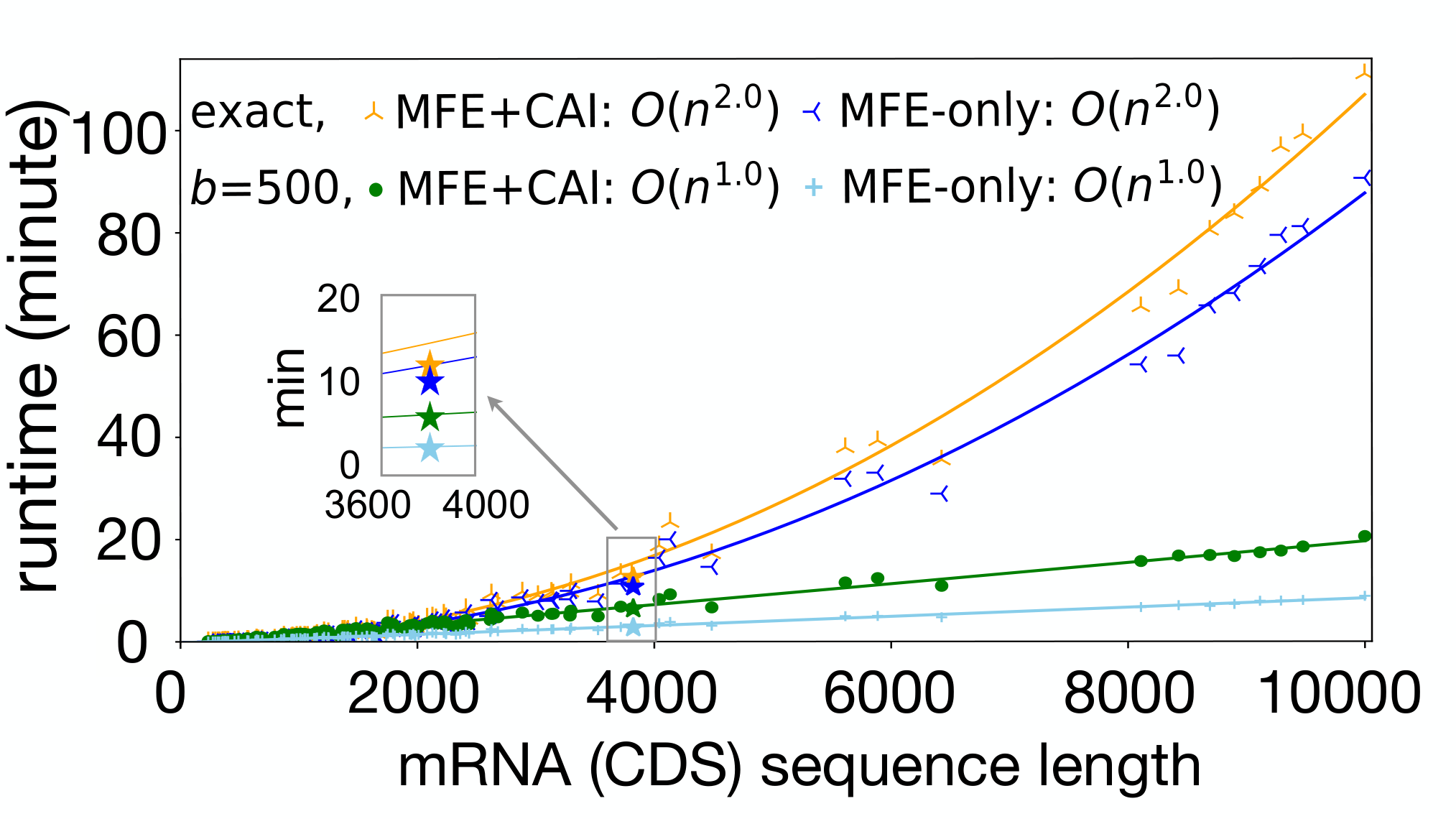
Fig. 3A benchmarked the runtime of LinearDesign on UniProt proteins [21]. LinearDesign was shown in a combination of two optimization objectives, MFE-only (objective 1) vs. MFE+CAI (objectives 1 & 2), and two search modes, exact search vs. beam search (beam size ). Empirically, LinearDesign scales quadratically with mRNA sequence length for practical applications ( nt) thanks to the DFA representation and lattice parsing (see Fig. S8 for analysis). Next, our CAI-integrated exact search (CAI weight ) had the same empirical complexity, and was only slower than the MFE-only version thanks to the convenience of adding CAI in our DFA representation. Last, our beam search version () further speeds up our design and scales linearly with sequence length, taking only 2.7 minutes (vs. 10.7 minutes for exact search) on the SARS-CoV-2 Spike protein (for MFE-only), with an approximation error (i.e., energy gap %, defined as ) of just 1.2%. In fact, as sequences get longer, this percentage stabilizes, suggesting that beam search quality does not degrade with sequence length; see Fig. S9 for details.
As shown in Figs. 3B–C, for a GC-favoring codon preference (such as human), the conventional codon optimization method does improve stability, but only slightly, since its optimization directions (the pink arrows) are largely orthogonal to the stability optimization directions (the blue arrows). By contrast, our LinearDesign can directly optimize stability and find the optimally stable mRNAs () on both the Spike protein and the enhanced gene fluorescent protein (eGFP), which have the lowest MFEs that are lower than the optimal-CAI’s (). Also, our optimally stable designs have mostly double-stranded secondary structures (Fig. 3D), which are predicted to be much less prone to degradation [5]. LinearDesign also finds the sequence with the lowest MFE for a given CAI and vice versa, thus forming the feasibility limit of mRNA design (the blue curves in Fig. 3B–C, with ranging from 0 to ). Furthermore, when the codon bias prefers AU-rich codons (such as yeast), codon optimization actually worsens stability (Fig. S10).
In vitro and In vivo Experimental Results
We performed experimental assays to study the chemical stability, protein expression, and immunogenicity of LinearDesign-generated mRNA molecules (Fig. 4). All mRNA sequences in this study encode the SARS-CoV-2 Spike protein without the 2P mutation [22], with unmodified (natural) nucleotides and the same UTRs. We used LinearDesign (with beam search plus a -best algorithm [23] for suboptimal candidates) to generate seven mRNA sequences ( a–g in Fig. 4A), which were compared to the benchmark sequence (baseline h ) designed by a commonly-used codon optimization algorithm, OptimumGene™. The seven LinearDesign sequences were selected to be widely distributed in the unexplored high-stability territory (the region in Fig. 4A where kcal/mol, inaccessible to codon optimization), and to separate the impacts of MFE and CAI, we designed sequences that are almost identical in either MFE (b–c // d–e–f) or CAI (a–c–f // b–e // d–g–h). It is well-known that translation efficiency drops if the 5’-leader region is particularly structured [5], so we did not optimize for the first 5 amino acids and used a heuristic to select the first 15 nucleotides. It is also suggested that long stems may induce unwanted innate immune responses [24], so we avoided them in our designs, which is why we did not study the lowest-MFE candidates closest to the optimal boundary (the blue curve) which usually contain long stems. See Methods §1.10 for details. It is worth mentioning that some UTR structures are crucial for translation [25], and we observe that our stable designs (a–f), having more structured coding regions, form fewer base pairs with, and thus interfere less with the structures of, commonly used UTRs than codon-optimized ones (Tab. S2). This suggests that LinearDesign is likely to be effective independent of the choice of UTRs.
In-solution Structure Compactness and Chemical Stability
 |
 |
|||||||||||||||||||||||||||||||||||||||||||||||||||||||||||||||||||||||||||||||||||||||||||||||||||||||||||||||||||||||||||||||||||||||||||||||||
| A | B | C | D | |||||||||||||||||||||||||||||||||||||||||||||||||||||||||||||||||||||||||||||||||||||||||||||||||||||||||||||||||||||||||||||||||||||||||||||||
| E | F | G | ||||||||||||||||||||||||||||||||||||||||||||||||||||||||||||||||||||||||||||||||||||||||||||||||||||||||||||||||||||||||||||||||||||||||||||||||
| H | ||||||||||||||||||||||||||||||||||||||||||||||||||||||||||||||||||||||||||||||||||||||||||||||||||||||||||||||||||||||||||||||||||||||||||||||||||
| ||||||||||||||||||||||||||||||||||||||||||||||||||||||||||||||||||||||||||||||||||||||||||||||||||||||||||||||||||||||||||||||||||||||||||||||||||
We then studied the structure compactness of mRNA molecules, which is hypothesized to be correlated with the folding free energy change. We performed Electrophoretic Mobility Shift Assay (EMSA) using Agarose gel electrophoresis at 30°C. An mRNA molecule with a lower MFE contains more secondary structures and thus exhibits more compact shape and smaller hydrodynamic size, which makes it move faster in the agarose gel matrix. We can see that the gel mobility pattern in Fig. 4B correlated with the MFEs of the eight designs almost perfectly: sequence a, with the lowest MFE, moved the fastest, followed by sequences b and c, then by sequences d, e, and f, then by sequence g, and finally by the baseline sequence h, which has the highest MFE.
To evaluate the chemical stability, we incubated the designed mRNA molecules in RNA storage buffer (Thermo Fisher) at 37°C followed by quantification of intact mRNA as a function of time. Overall, the chemical stability results also correlated well with the MFEs. The lowest-MFE design (a) degraded the slowest, and the highest-MFE baseline (h) the fastest, followed by the design (g) with the second highest MFE. For example, after day 4, there was only 2.8% intact molecules of h and 18.1% of g, while design a still had 36.9% and four other designs (b–d and f) also had around 30%. After day 5, sequence h had 0% remaining, sequence g had 8.8%, but the lower-MFE designs (a–f) still had 14.7%–19.2% left (Fig. 4C). These results suggest that low-MFE designs have longer half-lives, which will contribute to higher protein expression levels (see below).
Cellular Protein Expression
Sufficient antigen expression is one of the prerequisites for the induction of antibody responses so we evaluated the designed mRNA molecules for protein expression. The SARS-CoV-2 Spike protein is a transmembrane protein that can be directly detected on viable mRNA-transfected cells by flow cytometry. Following transfection into HEK-293 cells, we measured the amount of Spike proteins generated by all designs after 24 hours. Of note, 5 out of 7 mRNA molecules (designs a–d and g) showed substantially higher protein expression levels than the benchmark h (Fig. 4). For example, designs d and g (with CAIs almost identical to h, but lower MFEs) were 1.5 and 1.4 better, respectively, and the lowest MFE design a was also 1.5 better. In general, our results are consistent with Mauger et al.’s [5] that low MFE and high CAI synergize to improve protein expression, but we were able to test this hypothesis using mRNA molecules with much lower MFEs than they could, thanks to LinearDesign’s ability to explore the previously unreachable design space.
In vivo Immunogenicity
Ultimately, we tested whether our designs could endow mRNA vaccines with higher immunogenicity, which is usually represented by the magnitude of elicited antibody and T cell responses. We employed a lipid based delivery system for LinearDesign-generated mRNA vaccines [28], and further evaluated and compared the immunogenicity of each design side-by-side. C57BL/6 mice were intramuscularly immunized with two doses of vaccines at an interval of 2 weeks. Neutralizing antibodies, Spike protein-specific Immunoglobulin G (IgG), as well as antigen-specific interferon (IFN)--secreting T cells were assessed (see Fig. 4). Interestingly, all vaccine candidates carrying LinearDesign-generated mRNA molecules were able to elicit high levels of binding IgG and neutralizing antibodies. While in contrast, none or low levels of neutralizing antibodies were induced by the benchmark h. Similar results were also observed on the antigen-specific T cell response, where a robust T helper Type 1 (Th1)-biased T cell response was induced only by vaccines containing LinearDesign-generated mRNAs. Overall, our designs a–d, which are closer to the optimal boundary (shaded in Fig. 4A), i.e., strong in both MFE and CAI, led to a surprising increase in neutralizing antibody titers and increase in OD values for Spike-specific binding antibody than the benchmark (codon-optimized baseline h). These ratios were much higher than the corresponding ratios for cellular protein expression (), because the latter was only measured for 24 hours. We suspect that LinearDesign-generated mRNA molecules have longer functional half-lives in vivo (beyond 24 hours), which induce higher levels of antibody response.
Discussion
An effective mRNA design strategy is of utmost importance, especially for the development of mRNA vaccines that have shown great promise in fighting the current and future pandemics. However, it is extremely challenging due to the prohibitively large search space. We, instead, presented a surprisingly simple solution to this problem by formulating the design space as DFAs and reducing the mRNA design problem to lattice parsing in computational linguistics. This unexpected cross-disciplinary analogy provides an efficient algorithm that scales for practical applications, taking only 10.7 minutes for the SARS-CoV-2 Spike protein, and can jointly optimize stability and codon optimality using weighted DFAs. Our DFA framework can also apply to non-standard genetic codes, modified nucleotides, and coding constraints such as avoiding certain adjacent codon pairs. Finally, to provide suboptimal candidates for vaccine development and further speed up the design for long sequences, we provide an -time approximate variant.
The mRNA sequences generated by LinearDesign were comprehensively characterized in this study and demonstrated superiority over the commonly-used codon optimization benchmark in three attributes critical for vaccine performance: chemical stability, translation efficiency, and immunogenicity. In particular, four of our seven designs showed increase in neutralizing antibody titers and increase in binding antibody levels over the benchmark. Given that chemical modification is widely believed to be critical to the recent success of mRNA vaccines [29, 10, 1, 2],22 2 CureVac does not use modification either, but uses codon optimization and engineers the non-coding regions [3]; our algorithm is orthogonal to, and can be used with, their engineering efforts. it is intriguing that our designed mRNAs without chemical modification (with reduced cost in manufacturing) still showed high levels of stability, translation efficiency, and immunogenicity. On the other hand, our algorithm is orthogonal to chemical modification and can be combined with it once the corresponding energy model is available. By unleashing the previously inaccessible region of highly stable and efficient sequences, LinearDesign is a timely and promising tool for mRNA vaccine development which is of utmost importance to the current and future pandemics. But more importantly, it is also a general and principled method for molecule design in mRNA medicine, and can be used for all therapeutic proteins including monoclonal antibodies and anti-cancer drugs.
References
- [1] Baden LR, et al. (2021) Efficacy and safety of the mRNA-1273 SARS-CoV-2 vaccine. New England Journal of Medicine 384(5):403–416.
- [2] Polack FP, et al. (2020) Safety and efficacy of the BNT162b2 mRNA Covid-19 vaccine. New England Journal of Medicine.
- [3] Gebre MS, et al. (2021) Optimization of non-coding regions for a non-modified mRNA COVID-19 vaccine. Nature pp. 1–8.
- [4] Crommelin DJ, Anchordoquy TJ, Volkin DB, Jiskoot W, Mastrobattista E (2021) Addressing the cold reality of mRNA vaccine stability. Journal of Pharmaceutical Sciences 110(3):997–1001.
- [5] Mauger DM, et al. (2019) mRNA structure regulates protein expression through changes in functional half-life. Proceedings of the National Academy of Sciences U.S.A. 116(48):24075–24083.
- [6] Hall KB (2005) Best-first Word-lattice Parsing: Techniques for integrated syntactic language modeling. (Brown University).
- [7] Schlake T, et al. (2019) mRNA: a novel avenue to antibody therapy? Molecular Therapy 27(4):773–784.
- [8] Reinhard K, et al. (2020) An RNA vaccine drives expansion and efficacy of claudin-CAR-T cells against solid tumors. Science 367(6476):446–453.
- [9] Wolff JA, et al. (1990) Direct gene transfer into mouse muscle in vivo. Science 247(4949):1465–1468.
- [10] Pardi N, Hogan MJ, Porter FW, Weissman D (2018) mRNA vaccines—a new era in vaccinology. Nature Reviews Drug Discovery 17(4):261–279.
- [11] Kon E, Elia U, Peer D (2021) Principles for designing an optimal mRNA lipid nanoparticle vaccine. Current Opinion in Biotechnology 73:329–336.
- [12] Gustafsson C, Govindarajan S, Minshull J (2004) Codon bias and heterologous protein expression. Trends in Biotechnology 22(7):346–353.
- [13] Nabiyouni M, Prakash A, Fedorov A (2013) Vertebrate codon bias indicates a highly GC-rich ancestral genome. Gene 519(1):113–119.
- [14] Sahin U, Karikó K, Türeci Ö (2014) mRNA-based therapeutics—developing a new class of drugs. Nature reviews Drug discovery 13(10):759–780.
- [15] Sharp PM, Li WH (1987) The codon adaptation index-a measure of directional synonymous codon usage bias, and its potential applications. Nucleic Acids Research 15(3):1281–1295.
- [16] Durbin R, Eddy SR, Krogh A, Mitchison G (1998) Biological Sequence Analysis: Probabilistic Models of Proteins and Nucleic Acids. (Cambridge University Press, Cambridge, UK).
- [17] Bar-Hillel Y, Perles M, Shamir E (1961) On formal properties of simple phrase structure grammars. Zeitschrift für Phonetik, Sprachwissenschaft und Kommunikationsforschung 14(2):143–172.
- [18] Cohen B, Skiena S (2003) Natural selection and algorithmic design of mRNA. Journal of Computational Biology 10(3-4):419–432.
- [19] Terai G, Kamegai S, Asai K (2016) CDSfold: an algorithm for designing a protein-coding sequence with the most stable secondary structure. Bioinformatics 32(6):828–834.
- [20] Huang L, et al. (2019) LinearFold: linear-time approximate RNA folding by 5’-to-3’ dynamic programming and beam search. Bioinformatics 35(14):i295–i304.
- [21] Consertium U (2005) UniProt: a hub for protein information. Nucleic Acids Research 42:D204–D12.
- [22] Wrapp D, et al. (2020) Cryo-EM structure of the 2019-nCoV spike in the prefusion conformation. Science 367(6483):1260–1263.
- [23] Huang L, Chiang D (2005) Better k-best parsing. Proceedings of the Ninth International Workshop on Parsing Technologies pp. 53–64.
- [24] Liu L, et al. (2008) Structural basis of toll-like receptor 3 signaling with double-stranded RNA. Science 320(5874):379–381.
- [25] Mignone F, Gissi C, Liuni S, Pesole G (2002) Untranslated regions of mRNAs. Genome biology 3(3):1–10.
- [26] Jeong DE, et al. (2021) Assemblies of putative SARS-CoV2-spike-encoding mRNA sequences for vaccines BNT-162b2 and mRNA-1273 (version 0.1 beta 03/23/21).
- [27] Turner DH, Mathews DH (2010) NNDB: the nearest neighbor parameter database for predicting stability of nucleic acid secondary structure. Nucleic Acids Research 38(suppl_1):D280–D282.
- [28] Rana MM (2021) Polymer-based nano-therapies to combat COVID-19 related respiratory injury: progress, prospects, and challenges. Journal of Biomaterials Science, Polymer Edition pp. 1–31.
- [29] Karikó K, et al. (2008) Incorporation of pseudouridine into mRNA yields superior nonimmunogenic vector with increased translational capacity and biological stability. Molecular Therapy 16(11):1833–1840.
Availability
Web server: http://rna.baidu.com. Please contact rna@baidu.com if you need more advanced features.
Author Contributions
L.H. conceived and directed the project. L.H. designed the basic algorithm for the Nussinov model and wrote a Python prototype, and H.Z. and L.Z. extended this algorithm to the Turner model, and implemented it in C++, which Z.L. optimized. L.H., H.Z., and L.Z. designed the CAI integration algorithm which L.Z. and H.Z. implemented. L.Z. implemented the beam search and -best modules, and handled design constraints. K.L. made the webserver. B.L. implemented a baseline. Y.Z. supervised the in vitro and in vivo experiments. A.L., X.M., F.Z. performed the protein expression and immunogenicity assays, and C.X. performed chemical stability and structure compactness assays. D.H.M. discussed the approach and provided guidance for in silico analysis and writing. L.H., H.Z., L.Z., D.H.M., A.L., C.X., and Y.Z. wrote the manuscript. The work of H.Z., L.Z., K.L., and L.H. were done at Baidu Research USA.
Acknowledgments
We thank Rhiju Das (Stanford) for introducing the mRNA design problem to us, Robin Li (Baidu) for connecting Baidu Research with Stemirna, Julia Li (Baidu Research) for coordinating resources for this project, Goro Terai and Kiyoshi Asai (Univ. of Tokyo) for sending us the CDSfold code, Sharon Aviran (UC Davis) for spotting a typo in the hyperparameter in our earlier version, Alicia Solórzano (Pfizer) for the question on LinearDesign’s independence of the choice of UTRs, Jinzhong Lin (Fudan) for early discussions, and Sizhen Li (Oregon State Univ.) for proofreading and help on LaTeX. We thank Sanofi and many other vaccine companies worldwide for licensing and early adoption of LinearDesign. D.H.M. is supported by National Institutes of Health grant R01GM076485.
Methods
§1 Details of LinearDesign Algorithm
§1.1 Optimization Objectives
There are two objectives in mRNA design: stability and codon optimality. The optimal-stability mRNA design problem can be formalized as follows. Given a protein sequence where each is an amino acid residue, we find the optimal mRNA sequence that has the lowest minimum folding free energy change (MFE) among all possible mRNA sequences encoding that protein:
| (1) | |||||
| (2) |
where is the set of candidate mRNA sequences, is the set of all possible secondary structures for mRNA sequence , and is the free energy change of structure for mRNA according to an energy model. This is clearly a double minimization objective involving the per-sequence minimization over all of its possible structures (i.e., RNA folding; Eq. 2) which has well-known dynamic programming solutions, and the global minimization over all sequences (i.e., optimal mRNA design; Eq. 1) which we will solve using lattice parsing (§1.3).
Next, we integrate codon optimality by adding Codon Adaptation Index (CAI) [1], defined as the geometric mean of the codon optimality of each codon in the mRNA :
where is the th triplet codon in , and is the relative adaptiveness of codon , defined as the frequency of divided by the frequency of its most frequent synonymous codon (). Because CAI is always between 0 and 1 but MFE is generally proportional to the mRNA sequence length, we scale CAI by the number of codons and use a hyperparameter to balance MFE and CAI ( being purely MFE), and define a novel joint objective:
which can be simplified by expanding CAI:
| (3) | |||||
This joint objective is basically MFE plus (a scaled) sum of the negative logarithm of each codon’s relative adaptiveness. Now the joint optimization can be defined as:
See Fig. 2D for examples of relative adaptiveness calculation.
§1.2 DFA Representations for Codons and mRNA Candidate Sequences
Informally, a DFA is a directed graph with labeled edges and distinct start and end states. For our purpose each edge is labeled by a nucleotide, so that for each codon DFA, each start-to-end path represents a triplet codon. Formally, a DFA is a 5-tuple , where is the set of states, is the alphabet (here ), is the start state (always in this work), is the set of end states (in this work the end state is unique, i.e., ), and is the transition function that takes a state and a symbol and returns the next state , i.e., encodes a labeled edge .
After building DFAs for each amino acid, we can concatenate them into a single DFA for a protein sequence , which represents all possible mRNA sequences that translate into that protein
by stitching the end state of each DFA with the start state of the next. The new end state of the mRNA DFA is .
§1.3 Objective 1 (Stability): Stochastic Context-Free Grammar, Lattice Parsing, and Intersection
A stochastic context-free grammar (SCFG) is a context-free grammar in which each rule is augmented with a weight. More formally, an SCFG is a 4-tuple where is the set of non-terminals, is the set of terminals (identical to the alphabet in the DFA, in this case ), is the set of weight-associated context-free writing rules, and is the start symbol. Each rule in has the form where is a non-terminal that can be rewritten according to this rule into a sequence of non-terminals and terminals (the star ∗ means repeating zero or more times) and is the weight associated with this rule.
SCFGs are commonly used to represent the RNA folding energy model. The weight of a derivation (parse tree, or a secondary structure in this case) is the sum of weights of the productions used in that derivation [2]. For example, for a very simple Nussinov-Jacobson-style model [3], which simplifies the energy model to individual base pairs, we can define this SCFG as in Fig. S2E, where each gc pair gets a score of , and each au pair gets a score of . Thus, the standard RNA secondary structure prediction problem can be cast as a parsing problem: given the above SCFG and an input RNA sequence, find the minimum-weight derivation in that can generate the sequence. This can be solved by the classical CKY algorithm from computational linguistics [4, 5, 6].
The optimal-stability mRNA design problem is now a simple extension of the above single-sequence folding problem to the case of multiple inputs: instead of finding the minimum free energy structure (minimum weight derivation) for a given sequence, we find the minimum free energy structure (and its corresponding sequence) among all possible structures for all possible sequences (see Fig. S2). This can be solved by lattice parsing on the DFA, which is a generalization of CKY from a single sequence to a DFA. Take the bifurcation rule for example. In CKY, if you have derived non-terminal for span , notated , and if you have also derived , you can combine the two spans, i.e., , and use the above rule to derive . Similarly, in lattice parsing, if you have derived both (i.e., there is a path that can be derived from ) and , you can combine them to a longer path and derive with the above rule. While the runtime for CKY scales where is the grammar constant (the number of rules) and is the RNA sequence length, the runtime for lattice parsing similarly scales where is the number of states in the DFA. For mRNA design with the standard genetic code, because each position has either one or two states ( and ), so its time complexity is also actually identical to single-sequence folding, just with a larger constant. See Methods §1.6 for details of this algorithm and Figs. S3–S4 for the pseudocode.
More formally, in theoretical computer science, lattice parsing with an CFG on a DFA is also known as the intersection between the languages of and (i.e., the sets of sequences allowed by and ), notated , which was solved by the Bar-Hillel construction in 1961 [7]. In order to adapt it to mRNA design, we need to extend this concept to the case of weighted (i.e., stochastic) grammars and weighted DFAs (the latter is needed for CAI integration; see below). While the language of CFG is the set of sequences generated by , the language of the SCFG for RNA folding free energy model defines a mapping from each RNA sequence to its MFE, i.e., . This can be written as a relation:
And we also extend the language of a DFA to a trivial weighted language (which will facilitate the incorporation of CAI into DFA below):
Next we extend the intersection from two sets to two weighted sets and :
Now we can show that optimal-stability mRNA design problem can be solved via weighted intersection between and , i.e., we can construct a new “intersected” stochastic grammar that has the same weights (i.e., energy model) as the original grammar but only generates sequences in the DFA:
§1.4 Adding Objective 2 (Codon Optimality): Weighted DFA for CAI Integration
As described in the main text and Fig. 2D, our novel joint optimization objective (Eq. 3) factors the CAI of each mRNA candidate onto the relative adaptiveness of each of its codons, and thus can be easily incorporated into the DFA as edge weights. To do this we need to extend the definition of DFA to weighted DFA, where the transition function now returns a state and a weight, i.e., , which encodes a weighted label edge . Now the set of outgoing and incoming edges are also updated to:
In this case, the weighted DFA defines a mapping from each candidate mRNA sequence to its negative logarithm of CAI scaled by the number of codons, i.e., . More formally,
Now the weighted intersection defined above can be extended to incorporate the hyperparameter and derive the joint objective:
§1.5 Bottom-Up Dynamic Programming
Next, we describe how to implement the dynamic programming algorithm behind lattice parsing (or equivalently, intersection between the languages of a stochastic context-free grammar and a weighted DFA) to solve the joint optimization problem. For simplicity reasons, here we use bottom-up dynamic programming on a modified Nussinov-Jacobson energy model. Fig. S3 gives the pseudocode for this simplified version. We first build up the mRNA DFA for the given protein, and initialize two hash tables, to store the best score of each state, and to store the best backpointer. For the base cases (), we set for optimal-stability design, and for the joint optimization where
| (4) |
is the minimum (-scaled) cost of any path in the CAI-integrated DFA. Next, for each state it goes through the pairing rule and bifurcation rules, and updates if a better score is found. After filling out the hash tables bottom-up, we can backtrace the best mRNA sequence stored with the backpointers. See Fig. S4 for details of Update and Backtrace functions.
§1.6 Left-to-Right Dynamic Programming and Beam Search
Inspired by our previous work, LinearFold [8], we further developed a linear-time approximation algorithm for mRNA design. We apply beam pruning [9], a classical pruning technique, to significantly narrow down the search space without sacrificing too much search quality.
Fig. S5 gives the pseudocode of simplified LinearDesign algorithm for the Nussinov model, based on left-to-right dynamic programming and beam pruning. LinearDesign replaces bottom-up dynamic programming with a left-to-right parsing. At each step (the th position of mRNA sequence), we only keep the top states with the lowest cost and prune out the less promising states, since they are unlikely to be the optimal sequence. Here , the beam size, is a user-adjustable parameter to balance runtime and search quality. Notice that we use as default in LinearFold [20], but in LinearDesign we usually use a larger beam size of because the search space is larger.
Our real system uses a left-to-right dynamic programming with beam pruning on the Turner nearest neighbor free energy model [10, 11]. We implement the thermodynamic parameters following Vienna RNAfold [12], except for the dangling ends. Dangling ends refer to stabilizing interactions for multiloops and external loops[13], which require knowledge of the nucleotide sequence outside of the state . Though it could be integrated in LinearDesign, the implementation becomes more involved.
§1.7 DFAs for Other Genetic Codes, Coding Constraints, and Modified Nucleotides
The DFA framework can also represent less common cases such as alternative genetic codes, modified nucleotides, and coding constraints. First, DFA can encode non-standard genetic codes, such as alternative nuclear code for some yeast [14] and mitochondrial codes [15] (Fig. S6A). Second, we may want to avoid some unwanted or rare codons (such as the amber stop codon) which is an easy change on the codon DFAs (Fig. S6B), or certain adjacent codon pairs that modulate translation efficiency [16], which is beyond the scope of single codon DFAs but easy on the mRNA DFA (Fig. S6C). Similarly, we may want to disallow certain restriction enzyme recognition sites, which span across multiple codons (S7). Finally, chemically modified nucleotides such as pseudouridine () have been widely used in mRNA vaccines [17], which can also be incorporated in the DFA (Fig. S6D).
§1.8 Related Work
Two previous studies also tackled our objective 1 (optimal-stability mRNA design) via dynamic programming, but their algorithms are ad-hoc and complicated [18, 19]. By contrast, our work solves the harder and more general problem of joint optimization between stability and codon optimality (which subsumes their objective as a special case), yet using a much simpler and extendable solution. First, our work is the first to use automata theory to compactly and conveniently represent the exponentially large mRNA design space. Second, our reduction of mRNA design to lattice parsing induces a simple yet efficient solution based on classical results in computational linguistics and theoretical computer science, which scales rather than for practical applications (Figs. 3 & S8). Third, we define a novel joint optimization objective that factors the (logarithm of) CAI of an mRNA additively onto its individual codons, making it possible to incorporate codon optimality into dynamic programming. Codon usage is an important factor in mRNA design [20] that previous work was unable to jointly optimize.33 3 CDSfold [19] uses simulated annealing to improve CAI by fine-tuning from the MFE solution, but this is a heuristic with no guarantees, and their objective formulation, unlike ours, does not factor onto individual codons, thus cannot be incorporated into dynamic programming. Fourth, our DFA framework is so general that it can also represent arbitrary (non-standard) genetic codes, modified nucleotides, and coding constraints such as adjacent codon pair preference, which previous work could not handle even with major modifications. Fifth, we further develop a faster, linear-time, approximate version which greatly reduces runtime for long sequences with small sacrifices in search quality, which we also use to generate multiple suboptimal candidates with varying folding stability and codon optimality as candidates for experimentation. Last but not least, extensive experiments confirm that compared to the standard codon optimization benchmark, our designs are substantially better in chemical stability and protein expression in vitro, and the corresponding mRNA vaccines elicit up to 23 higher antibody responses in vivo (see Fig. 4).
§1.9 Benchmark Dataset and Machine
To estimate the time complexity of LinearDesign, we collected 114 human protein sequences from UniProt [21], with length from 78 to 3,333 amino acids (not including the stop codon). We benchmarked LinearDesign on a Linux machine with 2 Intel Xeon E5-2660 v3 CPUs (2.60 GHz) and 377 GB memory, and used Clang (11.0.0) to compile.
§1.10 Additional Design Constraints
Some studies have shown that protein expression level drops if the 5’-end leader region has more secondary structure [22, 23, 24, 25, 20]. To design sequences with less structures at 5’-end leader region, we take a simple “design, enumerate and concatenate” strategy to loose structure of the leader region: (1) design the CDS region except for the 5’-end leader region (i.e., the first 15 nucleotides); (2) enumerate all possible subsequences in the 5’-end leader region; and (3) concatenate each subsequence with the designed sequence, refold, and choose the one whose 5’-end leader region has the most unpaired nucleotides.
§2 Details of In vitro and In vivo Experiments
§2.1 Preparation of mRNA Vaccine
mRNA molecules were synthesized from corresponding linearized plasmid DNA template using T7 RNA polymerase, which flanked the open-reading frame (ORF) of Spike antigen with the 5’ and 3’ untranslated regions and a 70 poly-A tail. Cleancap analog was included to obtain capped RNA. The transcription reaction was incubated at 37°C for 6–8 hours, followed by treatment with DNase. RNA was then purified using Carboxylated microspheres. For the preparation of mRNA vaccines, lipopolyplex delivery platform was used to encapsulate the mRNA cargo as previously reported [29].
§2.2 Electrophoretic Mobility Shift Assay (EMSA) and Integrity assay of mRNA
To compare the electrophoretic mobility of mRNA molecules, mRNA samples were stored in Ambion® RNA storage buffer (Cat. # AM7001, Thermo Fisher, Mg2+ = 0mM). After denaturing at 70°C for 5 mins followed by cooling on ice, the mRNA samples were loaded on 1% agrose gel to run at 130V for 1h at 4°C. Gel image was taken by Gel Doc XR+ Gel Documentation System (Bio-Rad). (Fig. 4B)
RNA integrity was assayed by Qsep100TM Capillary Electrophoresis System. Intact mRNA was calculated as the percentage of full-length mRNA in solution. (Fig. 4C)
§2.3 Protein Expression Assay
Cell Culture
Human embryonic kidney (HEK)293T cells were cultured in Dulbecco’s modified Eagle’s medium (DMEM) (Hyclone) containing 10% fetal bovine serum (FBS) (GEMINI) and 1% Penicillin-Streptomycin (Gibco). All cells were cultured at 37°C in a 5% CO2 condition.
Measurement of Protein Expression from mRNA
Cells were transfected with mRNA molecules using Lipofectamine MessengerMAX (Thermo Scientific). Briefly, 2 of mRNA was mixed with 6 of Lipofectamine reagent first and then incubated with cells for 24 or 48 hours. For flow cytometric analysis, cells were collected and stained with live/dead cell dye (Fixable Viability Stain 510, BD) for 5 min. After washing, cells were incubated with anti-RBD chimeric mAb (1:100 dilution, Sino Biological) for 30 min, followed by washing and incubation with PE-anti-human IgG Fc (1:100 dilution, Biolgend) for 30 min. Samples were then acquired on BD Canto II (BD Biosciences). Data were analyzed using FlowJo V10.1 (Tree Star). (Fig. 4A and D)
§2.4 Immunization
C57BL/6 mice (6-8 weeks) were intramuscularly immunized twice with 10 of mRNA vaccines at a 2-week interval. Sera and spleens were collected 14 days after boost immunization. All experiments using mouse model were conducted under the ethical regulations and were approved by local ethical committees.
Surrogate Virus Neutralization (sVNT) Assay (Neutralizing Antibody Assay)
Neutralizing antibody titer was measured using sVNT assay as previously resported [30] with some modifications. Briefly, 96-well plates (Greiner Bio-one) were coated with hACE2 protein (100ng/well, Genscript) overnight at 4°C. Plates were washed with PBST and blocked with 2% BSA for 2 hours at RT. HRP-conjugated RBD (100 ng/ml) were incubated with serially diluted serum from immunized mice at an equal volume (60 each) for 30 min at 37°C. Sera collected from mice receiving PBS injection were used as negative control. Following this, a 100- mixture of RBD and serum was added into each well and incubated for 15 min at 37°C. After washing, TMB substrate (Invitrogen) was used for development and the absorbance was read at 450 nm using BioTek microplate reader. The IC50 value was calculated using 4 parameter logistic non-linear regression. (Fig. 4E)
Enzyme-linked Immunosorbent Assays (Binding Antibody Assay)
Recombinant SARS-CoV-2 Spike ectodomain protein (100 ng/well, Genscript) diluted in coating buffer (Biolegend) were coated into 96-well EIA/RIA plates (Greiner Bio-one) overnight at 4°C. The plates were then washed with PBS-T (0.05% Tween-20) and were blocked with 2% BSA in PBST for 2 hours at room temperature (RT). Serum samples (1:6400 diluted) were added and incubated for 2 hours at RT. After washing, total IgG was evaluated using HRP-conjugated goat anti-mouse IgG Ab (1:10,000) for 1 hour. TMB substrate (Invitrogen) was used for development and the absorbance was read at 450 nm using BioTek microplate reader. (Fig. 4F)
Enzyme-linked Immunospot (ELISpot) Assay (T Cell Response Assay)
Frequency of Spike antigen-specific IFN--secereting T cells was evaluated using Mouse IFN- ELISpotplus Kit (Mabtech) according to the manual. Briefly, 3105 murine splenocytes were added to wells pre-coated with anti-mouse IFN- capturing Abs and were incubated with Spike protein (10 ) for 20 hours. After washing, plates were incubated with Streptavidin-ALP (1:1000) for 1 hour at RT. Spots were developed with BCIP/NBT substrate solution and counted using Immunospot S6 analyzer (CTL). (Fig. 4G)
Supplementary Figures and Tables
| A | D | |
|
|
{forest} |
|
| B | C | |
| A B | |||
| C codon DFAs | D mRNA DFA |
| E stochastic grammar | F single-sequence folding | G from single-sequence folding to lattice parsing |
| H lattice parsing |
| A | ||
| alternative genetic code | ||
|
|
|
|
| B | |
| avoiding certain codon | |
|
|
|
| C | D | |
| avoiding a specific adjacent codon pair | chemically modified nucleotides | |
|
|
|
| A |
| B |
| C |
| A | B |
| of items generated bifurcation pairing in Nussinov model single-seq. folding CDSfold LinearDesign | |
| C | |
| A | B | C |
 |
 |
| A | B |

| sequence | MFE | Molecular | ||||
| of CDS | (kcal/mol) | CAI | GC% | U% | weight | |
| a | -2,287.3 | 0.756 | 54.8 | 22.7 | 1,229,541 | |
| b | -2,213.2 | 0.851 | 57.0 | 20.8 | 1,229,943 | |
| c | -2,206.0 | 0.757 | 55.3 | 22.2 | 1,230,380 | |
| d | -1,967.4 | 0.935 | 58.4 | 19.1 | 1,229,927 | |
| e | -1,961.3 | 0.851 | 56.8 | 21.1 | 1,229,328 | |
| f | -1,969.3 | 0.755 | 54.7 | 23.0 | 1,230,153 | |
| g | -1,639.3 | 0.935 | 58.6 | 18.9 | 1,229,526 | |
| h | -1,244.4 | 0.936 | 55.0 | 21.2 | 1,228,180 | |
| MFE-Optimal | -2,486.7 | 0.732 | 54.3 | 22.9 | 1,229,980 | |
| CAI-Optimal | -1,384.1 | 1.000 | 63.8 | 14.5 | 1,229,426 | |
| Wildtype | -966.7 | 0.655 | 37.3 | 33.3 | 1,221,872 | |
| CV2CoV | -1,384.4 | 0.903 | 63.9 | 15.7 | 1,226,373 | |
| mRNA-1273 | -1,369.2 | 0.978 | 62.3 | 15.5 | 1,229,366 | |
| BNT-162b2 | -1,217.2 | 0.946 | 57.0 | 19.1 | 1,227,844 |
| sequence | MFE | Stemirna UTRs | BioNTech UTRs | Moderna UTRs | CureVac UTRs | human -globin UTRs | |||||||||||||||
| of CDS | of CDS | MFE | tot. | 5’ | 3’ | MFE | tot. | 5’ | 3’ | MFE | tot. | 5’ | 3’ | MFE | tot. | 5’ | 3’ | MFE | tot. | 5’ | 3’ |
| kcal/mol | kcal/mol | kcal/mol | kcal/mol | kcal/mol | |||||||||||||||||
| a | -2287.3 | -2325.1 | 14 | 12 | 2 | -2378.0 | 8 | 5 | 3 | -2333.3 | 12 | 10 | 2 | -2313.4 | 5 | 5 | 0 | -2327.2 | 9 | 0 | 9 |
| b | -2213.2 | -2252.1 | 15 | 13 | 2 | -2302.0 | 5 | 5 | 0 | -2258.1 | 14 | 12 | 2 | -2235.7 | 5 | 5 | 0 | -2252.0 | 29 | 0 | 29 |
| c | -2206.0 | -2240.8 | 10 | 8 | 2 | -2294.1 | 6 | 6 | 0 | -2248.1 | 10 | 8 | 2 | -2229.7 | 17 | 17 | 0 | -2242.3 | 11 | 7 | 4 |
| d | -1967.4 | -2002.5 | 13 | 9 | 4 | -2056.4 | 10 | 5 | 5 | -2010.7 | 12 | 10 | 2 | -1991.8 | 3 | 0 | 3 | -2005.8 | 14 | 0 | 14 |
| e | -1961.3 | -1999.1 | 14 | 12 | 2 | -2057.3 | 15 | 5 | 10 | -2008.9 | 16 | 14 | 2 | -1989.6 | 19 | 12 | 7 | -2002.2 | 18 | 0 | 18 |
| f | -1969.3 | -2006.5 | 11 | 9 | 2 | -2060.9 | 11 | 5 | 6 | -2014.2 | 6 | 0 | 6 | -1993.8 | 11 | 0 | 11 | -2007.4 | 9 | 0 | 9 |
| g | -1639.3 | -1681.5 | 23 | 5 | 18 | -1743.0 | 33 | 4 | 29 | -1686.8 | 61 | 0 | 61 | -1673.4 | 22 | 22 | 0 | -1687.3 | 46 | 11 | 35 |
| h | -1244.4 | -1284.9 | 18 | 8 | 10 | -1345.3 | 72 | 8 | 64 | -1292.9 | 25 | 17 | 8 | -1285.5 | 27 | 19 | 8 | -1291.4 | 21 | 0 | 21 |
| CureVac | -1384.4 | -1424.4 | 21 | 5 | 16 | -1479.0 | 33 | 5 | 28 | -1430.5 | 82 | 26 | 56 | -1419.4 | 76 | 61 | 15 | -1425.5 | 20 | 0 | 20 |
| Moderna | -1369.2 | -1411.6 | 29 | 4 | 25 | -1464.3 | 24 | 4 | 20 | -1419.1 | 59 | 12 | 47 | -1406.6 | 63 | 45 | 18 | -1418.3 | 26 | 0 | 26 |
| BioNTech | -1217.2 | -1259.1 | 34 | 5 | 29 | -1316.3 | 98 | 6 | 92 | -1266.3 | 47 | 15 | 32 | -1253.9 | 58 | 54 | 4 | -1265.6 | 42 | 6 | 36 |
| MFE-opt. | -2486.7 | -2522.3 | 3 | 3 | 0 | -2575.9 | 1 | 1 | 0 | -2532.2 | 3 | 3 | 0 | -2512.5 | 2 | 2 | 0 | -2522.6 | 13 | 0 | 13 |
| CAI-opt. | -1384.1 | -1424.1 | 29 | 4 | 25 | -1478.0 | 58 | 0 | 58 | -1430.9 | 35 | 7 | 28 | -1420.4 | 53 | 53 | 0 | -1431.5 | 33 | 5 | 28 |
| Wildtype | -966.7 | -1007.0 | 21 | 19 | 2 | -1060.6 | 29 | 21 | 8 | -1019.1 | 27 | 25 | 2 | -1000.3 | 18 | 18 | 0 | -1011.7 | 56 | 9 | 47 |
References In Supplementary Materials
- [1] Sharp PM, Li WH (1987) The codon adaptation index-a measure of directional synonymous codon usage bias, and its potential applications. Nucleic Acids Research 15(3):1281–1295.
- [2] Rivas E (2013) The four ingredients of single-sequence RNA secondary structure prediction. a unifying perspective. RNA Biology 10(7):1185–1196.
- [3] Nussinov R, Jacobson AB (1980) Fast algorithm for predicting the secondary structure of single-stranded RNA. Proceedings of the National Academy of Sciences U.S.A. 77(11):6309–6313.
- [4] Kasami T (1966) An efficient recognition and syntax-analysis algorithm for context-free languages. Coordinated Science Laboratory Report no. R-257.
- [5] Younger DH (1967) Recognition and parsing of context-free languages in time . Information and Control 10(2):189–208.
- [6] Rivas E, Lang R, Eddy. R (2012) A range of complex probabilistic models for RNA secondary structure prediction that includes the nearest-neighbor model and more. RNA 18(2):193–212.
- [7] Bar-Hillel Y, Perles M, Shamir E (1961) On formal properties of simple phrase structure grammars. Zeitschrift für Phonetik, Sprachwissenschaft und Kommunikationsforschung 14(2):143–172.
- [8] Huang L, et al. (2019) LinearFold: linear-time approximate RNA folding by 5’-to-3’ dynamic programming and beam search. Bioinformatics 35(14):i295–i304.
- [9] Huang L, Fayong S, Guo Y (2012) Structured perceptron with inexact search in Proceedings of the 2012 Conference of the North American Chapter of the Association for Computational Linguistics: Human Language Technologies. (Association for Computational Linguistics, Montréal, Canada), pp. 142–151.
- [10] Mathews DH, Sabina J, Zuker M, Turner DH (1999) Expanded sequence dependence of thermodynamic parameters improves prediction of RNA secondary structure. Journal of Molecular Biology 288(5):911–940.
- [11] Mathews DH, et al. (2004) Incorporating chemical modification constraints into a dynamic programming algorithm for prediction of RNA secondary structure. Proceedings of the National Academy of Sciences U.S.A. 101(19):7287–7292.
- [12] Lorenz R, et al. (2011) ViennaRNA package 2.0. Algorithms for Molecular Biology 6(1):1.
- [13] Turner DH, Mathews DH (2010) NNDB: the nearest neighbor parameter database for predicting stability of nucleic acid secondary structure. Nucleic Acids Research 38(suppl_1):D280–D282.
- [14] Kawaguchi Y, Honda H, Taniguchi-Morimura J, Iwasaki S (1989) The codon CUG is read as serine in an asporogenic yeast candida cylindracea. Nature 341(6238):164–166.
- [15] Bonitz SG, et al. (1980) Codon recognition rules in yeast mitochondria. Proceedings of the National Academy of Sciences U.S.A. 77(6):3167–3170.
- [16] Gamble CE, Brule CE, Dean KM, Fields S, Grayhack EJ (2016) Adjacent codons act in concert to modulate translation efficiency in yeast. Cell 166(3):679–690.
- [17] Karikó K, et al. (2008) Incorporation of pseudouridine into mRNA yields superior nonimmunogenic vector with increased translational capacity and biological stability. Molecular Therapy 16(11):1833–1840.
- [18] Cohen B, Skiena S (2003) Natural selection and algorithmic design of mRNA. Journal of Computational Biology 10(3-4):419–432.
- [19] Terai G, Kamegai S, Asai K (2016) CDSfold: an algorithm for designing a protein-coding sequence with the most stable secondary structure. Bioinformatics 32(6):828–834.
- [20] Mauger DM, et al. (2019) mRNA structure regulates protein expression through changes in functional half-life. Proceedings of the National Academy of Sciences U.S.A. 116(48):24075–24083.
- [21] Consertium U (2005) UniProt: a hub for protein information. Nucleic Acids Research 42:D204–D12.
- [22] Ding Y, et al. (2013) In vivo genome-wide profiling of RNA secondary structure reveals novel regulatory features. Nature 505.
- [23] Wan Y, et al. (2014) Landscape and variation of RNA secondary structure across the human transcriptome. Nature 505:706–709.
- [24] Shah P, Ding Y, Niemczyk M, Kudla G, Plotkin JB (2013) Rate-limiting steps in yeast protein translation. Cell 153:1589–601.
- [25] Tuller T, Zur H (2014) Multiple roles of the coding sequence 5’ end in gene expression regulation. Nucleic Acids Research 43(1):13–28.
- [26] Liu L, et al. (2008) Structural basis of toll-like receptor 3 signaling with double-stranded RNA. Science 320(5874):379–381.
- [27] Husain B, Mukerji I, Cole JL (2012) Analysis of high-affinity binding of protein kinase R to double-stranded RNA. Biochemistry 51(44):8764–8770.
- [28] Hur S (2019) Double-stranded RNA sensors and modulators in innate immunity. Annual Review of Immunology 37:349–375.
- [29] Persano S, et al. (2017) Lipopolyplex potentiates anti-tumor immunity of mRNA-based vaccination. Biomaterials 125:81–89.
- [30] Tan CW, et al. (2020) A SARS-CoV-2 surrogate virus neutralization test based on antibody-mediated blockage of ACE2–spike protein–protein interaction. Nature Biotechnology 38(9):1073–1078.
- [31] Ohama T, et al. (1993) Non-universal decoding of the leucine codon CUG in several Candida species. Nucleic Acids Research 21(17):4039–4045.
- [32] Shulgina Y, Eddy SR (2021) A computational screen for alternative genetic codes in over 250,000 genomes. eLife 10:e71402.
- [33] Fredens J, et al. (2019) Total synthesis of Escherichia coli with a recoded genome. Nature 569(7757):514–518.