AMP-Net: Denoising based Deep Unfolding for Compressive Image Sensing
Abstract
Most compressive sensing (CS) reconstruction methods can be divided into two categories, i.e. model-based methods and classical deep network methods. By unfolding the iterative optimization algorithm for model-based methods onto networks, deep unfolding methods have the good interpretation of model-based methods and the high speed of classical deep network methods. In this paper, to solve the visual image CS problem, we propose a deep unfolding model dubbed AMP-Net. Rather than learning regularization terms, it is established by unfolding the iterative denoising process of the well-known approximate message passing algorithm. Furthermore, AMP-Net integrates deblocking modules in order to eliminate the blocking artifacts that usually appear in CS of visual images. In addition, the sampling matrix is jointly trained with other network parameters to enhance the reconstruction performance. Experimental results show that the proposed AMP-Net has better reconstruction accuracy than other state-of-the-art methods with high reconstruction speed and a small number of network parameters.
Index Terms:
compressive sensing, deep unfolding, approximate message passing, image denoising, image reconstruction.I Introduction
Compressive sensing (CS) requires much fewer measurements than the classical Nyquist sampling to reconstruct a signal [1]. It has been applied in a series of imaging applications, including single-pixel camera [2], magnetic resonance imaging (MRI) [3], and snapshot compressive imaging (SCI) [4].
CS performs fast imaging by sampling few measurements, i. e. , where is the original signal, consists of the samples, is the sampling matrix with . The image recovery from compressive samples is to solve an under-determined linear inverse system, and the corresponding optimization model can be formulated as follows:
| (1) |
where is the regularization term.
To solve this optimization problem, model-based recovery methods exploit some data structures by employing structure-inducing regularizers [5], such as sparsity in some transformation domains [6, 7, 8, 9], low rank [10, 11, 12, 13, 14, 15], and so on [16, 17, 18, 19, 20]. A number of non-linear iterative algorithms can be used to solve these optimization problems [21, 22, 11], such as sparse Bayesian learning [23], orthogonal matching pursuit (OMP) [24], fast iterative shrinkage-thresholding algorithm (FISTA) [25], approximate message passing (AMP) [26], etc. These methods usually have theoretical guarantees.
In these years, some deep-learning-based methods have been developed for the image recovery problem [27]. Classical deep networks directly map the compressive samples as input to the estimations as output [28, 29, 30, 31, 32]. These networks consist of stacked non-linear operational layers, such as autoencoders [29], convolutional neural networks (CNNs) [33], generative adversarial networks (GANs) [34], etc. Their parameters can be trained by the well-known backpropagation algorithm. Compared with the iterative optimization algorithms, these classical deep neural networks can quickly reconstruct images. Nevertheless, due to the black box characteristic of these models, there is no good interpretation and theoretical guarantee. These completely data-driven end-to-end manners may have risks for some undesired effects [35]. Therefore, it can be beneficial to integrate the prior knowledge and the structure of the operators.
Motivated by the iterative algorithm that processes data step by step, deep unfolding maps iterative restoration algorithms onto deep neural networks [36, 37, 38, 39]. It tries to make a compromise between the iterative recovery methods and network methods, and enjoys a good balance between reconstruction speed and interpretation. Deep unfolding methods are first developed to solve the sparse linear inverse problem and the unfolded algorithms include ISTA [36, 40], AMP [41] and iterative hard thresholding (IHT) algorithm [42]. However, it is usually necessary for these methods to obtain additional pre-trained dictionaries to recover images.

In recent years, some non-linear iterative algorithms are unfolded to solve image CS problems. For example, ADMM is unfolded for MRI [38] and SCI [4], and the primal-dual algorithm is developed to reconstruct CT [43]. AMP [44] and ISTA [37] are exploited to reconstruct visual images. And the half-quadratic splitting (HQS) algorithm [39] and the linear inverse operation [45] are developed to solve common image inverse problems. Some methods [38, 4, 37] design deep unfolding models by pre-assuming specific regularizers, such as norm for sparsity in some basis. Carefully designed regularization terms are intuitive, but may ignore other image intrinsic structures. It has been proved that combining multiple kinds of image prior knowledge can get better reconstruction results than single one [12, 13, 46]. To integrate more information, some methods use deep networks to model an appropriate regularizer [37, 43, 39, 45]. But due to the uncertainty and unrepresentability of the regularizer, it is difficult to learn the regularizer directly. Instead, some information related to the regularizer is learned, such as denoising prior [39], gradient [47], inverse information [45]. However, to learn this information, classical deep neural networks usually contain a large number of parameters, which makes the application of related models limited. In this paper, we establish the deep unfolding model by unfolding the iterative denoising process from the denoising perspective of the AMP algorithm.
The AMP algorithm interprets a classical linear operation as the sum of the original data and a noise term [26], where is an estimate of . To obtain the original data, related non-linear operations in each iteration can be regarded as a series of denoising processes which depend on different image priors. In this paper, we call this interpretation the denoising perspective of the AMP algorithm. Based on this theory, [44] employs CNNs for denoising or approximating the bias named Onsager correction term. However, the denoiser is designed without considering the sampling matrix. In this paper, we analyze the noise term in more detail, and combine CNNs and the sampling matrix to fit the noise term jointly. Furthermore, based on that, a control parameter can be introduced to enhance the flexibility of the reconstruction. Such a strategy makes the representation of the image prior more flexible and intuitive with fewer demanded parameters.
Besides, in CS systems, some methods [48, 29, 30, 37] sample and reconstruct images block-by-block. This strategy brings less burden to the hardware. However, for these block-based methods, additional deblocking operations must be applied to eliminate blocking artifacts. Some methods [29, 30] use artificial deblockers to erase the artifacts, such as BM3D. Some classical deep networks perform image reconstruction and deblocking at the same time [31, 32]. In this paper, we propose a trainable deblocking module, which not only can be used in AMP-Net, but also can be plugged in other deep learning methods.
In addition, recently the sampling matrix optimization is employed in some model-based methods and classical deep neural networks [20, 30, 31, 49, 50], which are designed for image CS[20, 30, 31, 50] and video CS[49]. In such a strategy, the sampling matrix is trained with other parameters using gradient descent way related algorithms [51]. By limiting the value of the sampling matrix, different forms of sampling matrices can be obtained, including floating-point matrix [20, 30, 31], sparse matrix [50] and binarized matrix [31, 49]. In this paper, we focus on the trained floating-point matrix. Since the sampling matrix plays an important role in both sampling and reconstruction in most deep unfolding methods [37, 39, 45], an appropriate sampling matrix may effectively improve the reconstruction performance. In this work, we jointly train the sampling matrix with other parameters of the designed deep unfolding model.
In general, in this paper, we propose a novel deep unfolding model dubbed AMP-Net to solve the visual image CS problem. Fig. 1 illustrates the framework of AMP-Net. AMP-Net is composed of a sampling model and a reconstruction model. In the sampling model, images are measured block-by-block using the same sampling matrix. The reconstruction model is established by unfolding the iterative denoising process, which is inspired by the denoising perspective of the AMP algorithm. The reconstruction model is an unfolding form of the denoising process with iterations. It consists of an initialization module and reconstruction modules. The initialization module is used to generate a reasonable initial estimation. Each reconstruction module contains a denoising module and a deblocking module. The denoising module processes each image block, and the deblocking module is for the whole image. Experimental results demonstrate that the proposed method outperforms the state-of-the-art ones in terms of reconstruction accuracy and computational complexity.
The main contributions of this paper can be summarized as follows:
- •
We develop a novel deep unfolding model named AMP-Net which is inspired by the denoising perspective of the AMP algorithm. With a detailed analysis of the noise term, we integrate CNNs and the sampling matrix for accurate noise estimation.
- •
To eliminate the blocking artifacts, a trainable deblocking module is designed following the denoising module. To the best of our knowledge, this is the first work which learns deblockers and integrates them into a deep unfolding model. And experimental results reveal that this strategy also benefits other deep learning methods.
- •
In AMP-Net, the sampling matrix is trained with other parameters jointly due to its contributions in both sampling and reconstruction. In this way, the produced optimized matrix is data-driven and provides performance improvement not only for AMP-Net but for other reconstruction methods.
II Background
In this section, the denoising perspective of the AMP algorithm is introduced and some works related to AMP-Net are presented.
II-A The Denoising Perspective of the AMP Algorithm
The AMP algorithm analyzes a classical scheme of iterative non-linear algorithms [25, 26] as follows:
| (2) | ||||
| (3) |
where is the transpose of sampling matrix , is the non-linear function, and is the number of the iteration. If the initialized input and the original data are defined as and , then we can have
| (4) |
where is the identity matrix in the size of . The detailed derivation of (4) can be found in Appendix A. By extending (4) to the -th iteration, we can get
| (5) |
where the entries of the sampling matrix are independent and identically distributed as , and denotes the Gaussian distribution with the mean value and the variance . Under this assumption, it can be proved that is also a Gaussian distributed vector with the variance [26]. Then, (5) can be reformulated into the sum of the original signal and a noise term as follows:
| (6) |
where denotes the noise term.
The AMP algorithm interprets the non-linear function as a denoising function varying with different signal priors. For example, if signals are assumed to be sparse without value limitation, can be the soft thresholding function [25]. In this paper, we call such interpretation as the denoising perspective of the AMP algorithm.
Significantly, it is worth noting that has no relation with the regularizer in model-based methods. It is only affected by the original image and the input of each iteration. Therefore, it can be fitted by supervised learning, while the image prior can be learned in the noise term learning process. Such a strategy makes the representation of the image prior more flexible and intuitive with no need to figure out the specific form of the regularization term. And it can be noticed that if decreases in each iteration, the Euclidean distance between the reconstruction result and would get smaller as the iteration number increases.
II-B Related Works
Model-based methods are based on regularization terms inspired by image priors. Sparsity in some transformation domains, such as DCT [6], wavelet [52] and gradient domain [48], has been exploited to reconstruct visual images. For example, Li et al. [48] used a second order total variation (TV) regularizer to build an optimization problem and applied the augmented Lagrangian method to recover each image block. However, the fixed domain may result in poor performance. To improve the reconstruction performance, some elaborate priors have been exploited, such as denoising prior [17, 18] and network prior [19, 20]. Specifically, Metzler et al. [17] combined the BM3D denoiser with the AMP algorithm to develop a new framework named D-AMP for image reconstruction. And Wu et al. [20] employed a pre-trained deep neural network to represent the image prior and applied three times of gradient descend to reconstruct images. In this framework namely DCS, the sampling matrix is pre-trained.
For classical deep network methods, Mousavi et al. [29] designed a stacked denoising autoencoder (SDA) to reconstruct images from sampled data for the first time. After that, Lohit et al. [30] proposed a CNN-based model namely ReconNet to improve the reconstruction performance of visual images, where a popular denoiser called BM3D is employed for image deblocking in postprocessing. Shi et al. [31] proposed a novel sampling-reconstruction framework named CSNet based on residual CNNs. Although the sampling matrix can be jointly trained with the reconstruction model in these three methods, it is not integrated into the reconstruction model. For example, CSNet directly replaces the sampling model with a convolutional layer, which is not considered in the following reconstruction model. However, in AMP-Net, the sampling matrix plays an important role in the reconstruction model. And by training the sampling matrix, while producing better measurements, the performance of the reconstruction model can be further improved.
Deep unfolding methods combine the advantages of model-based methods and classical deep network methods. For example, the popular algorithm ISTA is unfolded as ISTA-Net [37], which is commonly used to solve optimization problems with a sparsity-inducing regularizer. It employs CNNs to learn the appropriate transformation operations and trainable soft thresholding functions to reflect the sparsity of data. Gilton et al. [45] developed a deep unfolding model named Neumann Network (NN) for common image inverse problems by truncating Neumann series with a data-driven non-linear regularizer.
Similar to AMP-Net, three methods namely DPDNN, LDIT and LDAMP apply denoising priors. Dong et al. [39] designed a deep unfolding model dubbed DPDNN to solve common inverse problems, which unfolds the denoising process inspired by HQS algorithm. In each reconstruction module of DPDNN, the deep neural network aims to learn the information of the regularizer, and two parameters are introduced to control the step size and the trade-off between the regularizer and the data fitting term. However, AMP-Net applies deep neural networks for noise approximation and introduces only one control parameter.
Metzler et al. [44] proposed LDIT and LDAMP inspired by the denoising-based iterative thresholding (DIT) algorithm and the AMP algorithm respectively. And different from LDIT, LDAMP introduces an addictive bias term named Onsager correction term before denoising. The main difference between the proposed AMP-Net and LDIT or LDAMP is the method for noise estimation. LDIT and AMP-Net both try to estimate the noise term which is formulated as . However, they employ different estimation strategies. In detail, LDIT employs a CNN to estimate the entire noise term directly, but AMP-Net uses a CNN to fit only and then multiplies the sampling matrix to estimate the noise. In addition, a trainable parameter is introduced to improve the flexibility of AMP-Net.
III AMP-Net
In this section, we will illustrate the detail of AMP-Net. As shown in Fig. 1, AMP-Net is composed of a sampling model and a reconstruction model which contains an initialization module and a series of stacked reconstruction modules.
Note that we mainly focus on single-channel images in this study while colorful images can be sampled and recovered channel by channel.
III-A Sampling Model
The sampling model samples images block-by-block and is similar to the one in CSNet [31]. However, it is not composed of convolutional kernels but a simple sampling matrix due to its relevance to the reconstruction process.
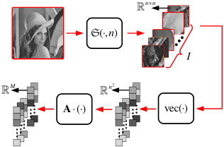
To demonstrate the sampling process, we denote as a splitting function which divides a single-channel image as into a series of non-overlapping image blocks. Each image block is denoted as , where and . And is defined as a vectorization function which vectorize an image block to a vector, and satisfies and . The sampling process of the sampling model is shown in Fig. 2 and can be expressed as
| (7) |
where is the sampling matrix for image blocks and is the measurement. Each column of is the vectorized measurement of an image block.
Moreover, in order to further improve the performance of AMP-Net, is simultaneously trained with other parameters for its contributions in both sampling and reconstruction. And the derivation of its gradient for updating can refer to Appendix B.
III-B Reconstruction Model
Due to the inspiration of the denoising perspective of the AMP algorithm, the reconstruction model is established by unfolding the iterative denoising process. This model is composed of an initialization module and a series of reconstruction modules. The initialization module is used to generate a reasonable initial estimation. The subsequent reconstruction modules are derived by mapping the iterative denoising process onto a deep network. Each module stands for an iteration. And each reconstruction module contains a denoising module and a deblocking module.

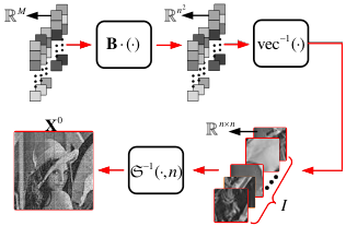
Initialization module. The image is initialized by linear operations of the observations. Fig. 3 shows the initialization process. is defined as a concatenation function which merges all the image blocks into a whole image and satisfies . Meanwhile, is a reshaping function which reshapes the vectorized image to its original shape and satisfies . The initialization process can be formulated as
| (8) |
where is a trainable matrix for initialization and denotes the initialized image.
Denoising module. The denoising module is designed to reconstruct each image block. By assuming that and inspired by (5), the original data can be obtained by calculating
| (9) |
If is obtained, the reconstruction can be achieved by linear operations. To this end, we replace with a non-linear trainable function and extend (III-B) to an iterative version, which can be expressed as
| (10) |
By regarding as the noise term, the reconstruction process in (III-B) can be interpreted as the denoising process. And because is used to fit , the noise term is not limited to the Gaussian noise.
Moreover, a trainable parameter is introduced to enhance the flexibility of the reconstruction process. With , the iterative reconstruction process can be expressed as
| (11) |
The detailed derivation of (III-B) is similar to (III-B) and can be found in Appendix C. Significantly, is similar to the step size in other deep unfolding algorithms [40, 37], but it is a parameter to control the noise and the reconstruction ability of the module in this paper. Therefore, is named as the control parameter, and (III-B) would degenerate to (III-B) when equals 1.
In this paper, is designed to be a CNN. As shown in Fig. 4, is constructed of four convolutional layers, of which the first three layers with bias terms are followed by the Rectified Linear Unit (ReLU) [53] and the last convolutional layer has no bias term. The filter size of each convolutional layer is . To make sure that the output has the same size as the input, the padding size of each convolutional layer is set to be 1. The numbers of output channels of the four convolutional layers are 32, 32, 32 and 1, respectively.
By extending (III-B) to the reconstruction of the whole image, the mathematical expression of the denoising module of the -th reconstruction module is as follows:
| (12) |
where
| (13) | ||||
| (14) |
And Fig. 4 provides a graphical illustration of the -th reconstruction module of AMP-Net.
As we can see, plays an important role in the reconstruction process (III-B). If there is an appropriate sampling matrix, the reconstruction performance would get improved. This probably partly explains why the sampling matrix training strategy is effective for recovery. Furthermore, we emphasize that , , and do not introduce additional floating-point calculations.
Deblocking module. Reconstructing images block-by-block without overlapping may lead to a situation that additional deblocking operations must be carried out. Some methods [29, 30] use hand-crafted denoisers to deblock images. However, artificial denoisers may ignore some semantic information that is helpful for deblocking. In this paper, a trainable deblocking module is developed to eliminate the blocking artifacts and further improve the reconstruction performance.
| Method | Trainablity | Interpretation | Fixed computational | Sampling matrix | Deblocking | Regularization |
|---|---|---|---|---|---|---|
| complexity | training | operation | term | |||
| TVAL3 [48] | ||||||
| D-AMP [17] | ||||||
| DCS [20] | ||||||
| ReconNet [30] | ||||||
| [31] | ||||||
| [37] | ||||||
| LDIT [44] | ||||||
| LDAMP [44] | ||||||
| DPDNN [39] | ||||||
| NN [45] | ||||||
| AMP-Net |
In detail, can be further expressed as where denotes the additive blocking artifacts from the -th denoising module. To map to , a non-linear learnable function is designed to fit . With the similar structure of ResNet [54], the process of image deblocking in the -th reconstruction module is illustrated in Fig. 4 and can be expressed as
| (15) |
where and denote the input and the output, respectively. The input of is the whole concatenated image rather than each image block. In fact, is a CNN with the same structure as in this study but different parameter values. Significantly, this process can also be regarded as the further denoising of the image, and processing the whole image gives AMP-Net the potential of image deblocking.
Input: , , , , , , ,
Output: output
Sampling process:
Reconstruction process:
III-C Loss Function
In this paper, for easy reference, AMP-Net- is named as the AMP-Net with denoising modules. AMP-Net--B is AMP-Net- with deblocking modules and AMP-Net--M is AMP-Net- with the sampling matrix training strategy. And AMP-Net--BM is AMP-Net- with both of them.
The trainable parameters of AMP-Net--BM contain the measurement matrix , initialization matrix , the control parameters , all the trainable parameters in set as , and all the trainable parameters in set as . denotes the trainable parameters of and denotes the trainable parameters of . Algorithm 1 describes the forward propagation of AMP-Net--BM.
In this paper, we use mean square error (MSE) to describe the difference between the original image and the recovered image. Then the loss function of AMP-Net--BM can be formulated as
| (16) |
where is the -th original image in the training set, denotes the size of and denotes the size of the training set. We emphasize that the forward propagation processes and the loss functions of AMP-Net-, AMP-Net--B and AMP-Net--M can be easily derived from Algorithm 1 and (16) by erasing some elements.
IV Experimental Results
In this section, numerical experiments are performed on the visual image CS reconstruction. Firstly, the effectiveness of the unfolding strategy, deblocking module and sampling matrix learning strategy of AMP-net is validated individually in section IV-B, IV-C and IV-D. Then the performance of AMP-Net with blocking modules and the sampling matrix optimization is compared with some state-of-the-art reconstruction methods.
| Method | 50 | 40 | 30 | 25 | 10 | 4 | 1 |
|---|---|---|---|---|---|---|---|
| PSNR (dB)/SSIM | |||||||
| TVAL3 | 33.39/0.8157 | 31.21/0.7531 | 29.00/0.6764 | 27.63/0.6238 | 22.45/0.3758 | 17.88/0.1997 | 14.90/0.0646 |
| D-AMP | 37.34/0.8504 | 35.22/0.8078 | 32.64/0.7544 | 31.62/0.7233 | 19.87/0.3757 | 11.28/0.0971 | 5.58/0.0034 |
| ReconNet | 32.12/0.9137 | 30.59/0.8928 | 28.72/0.8517 | 28.04/0.8303 | 24.07/0.6958 | 21.00/0.5817 | 17.54/0.4426 |
| LDIT | 37.06/0.9626 | 34.92/0.9470 | 32.69/0.9223 | 31.35/0.9042 | 25.56/0.7691 | 21.45/0.6075 | 17.58/0.4449 |
| LDAMP | 35.90/0.9531 | 34.07/0.9383 | 32.01/0.9144 | 29.93/0.8783 | 24.94/0.7483 | 21.30/0.5985 | 17.51/0.4409 |
| DPDNN | 35.85/0.9532 | 34.30/0.9411 | 32.06/0.9145 | 30.63/0.8924 | 24.53/0.7392 | 21.11/0.6029 | 17.59/0.4459 |
| NN | 31.41/0.8871 | 29.51/0.8523 | 27.64/0.8095 | 26.57/0.7842 | 22.99/0.6591 | 20.65/0.5525 | 17.67/0.4324 |
| 38.08/0.9680 | 35.93/0.9537 | 33.66/0.9330 | 32.27/0.9167 | 25.93/0.7840 | 21.14/0.5947 | 17.48/0.4403 | |
| AMP-Net-6 | 37.48/0.9650 | 35.27/0.9495 | 32.96/0.9254 | 31.71/0.9090 | 25.72/0.7750 | 21.52/0.6100 | 17.53/0.4426 |
| AMP-Net-9 | 37.78/0.9667 | 35.63/0.9523 | 33.40/0.9307 | 32.05/0.9140 | 25.93/0.7828 | 21.69/0.6224 | 17.58/0.4397 |
| Method | 50 | 40 | 30 | 25 | 10 | 4 | 1 |
|---|---|---|---|---|---|---|---|
| PSNR (dB)/SSIM | |||||||
| ReconNet | 30.85/0.8949 | 29.47/0.8647 | 27.95/0.8190 | 27.20/0.7914 | 23.98/0.6472 | 21.69/0.5557 | 18.96/0.4531 |
| LDIT | 34.27/0.9453 | 32.23/0.9184 | 30.23/0.8799 | 29.10/0.8523 | 24.94/0.7040 | 22.04/0.5759 | 19.00/0.4564 |
| LDAMP | 33.45/0.9359 | 31.79/0.9116 | 29.89/0.8724 | 28.35/0.8297 | 24.61/0.6920 | 21.93/0.5721 | 18.94/0.4512 |
| DPDNN | 33.56/0.9373 | 32.05/0.9164 | 29.98/0.8759 | 28.87/0.8491 | 24.37/0.6863 | 21.80/0.5716 | 18.97/0.4544 |
| NN | 30.47/0.8882 | 28.84/0.8511 | 27.23/0.8037 | 26.42/0.7757 | 23.44/0.6443 | 21.49/0.5451 | 19.06/0.4474 |
| 34.92/0.9510 | 32.87/0.9264 | 30.77/0.8901 | 29.64/0.8638 | 25.11/0.7124 | 21.82/0.5661 | 18.92/0.4529 | |
| AMP-Net-6 | 34.55/0.9478 | 32.50/0.9223 | 30.43/0.8840 | 29.33/0.8574 | 25.02/0.7095 | 22.09/0.5779 | 18.99/0.4543 |
| AMP-Net-9 | 34.79/0.9504 | 32.75/0.9253 | 30.67/0.8887 | 29.53/0.8625 | 25.12/0.7153 | 22.22/0.5851 | 18.97/0.4541 |
IV-A Experimental settings
All of our experiments are performed on two datasets: BSDS500 [55] and Set11 [30]. BSDS500 contains 500 colorful visual images which are divided into three parts: the training set (200 images), the validation set (100 images) and the test set (200 images). And Set11 [30] contains 11 grey-scale images. We use the luminance components of BSDS500 for training, validation and testing, and use Set11 for testing.
In this study, we set the size of each image block as 33. Two training sets are generated for models with and without trainable deblocking operations respectively. (a) Training set 1: 448 sub-images with the size are randomly extracted from the luminance component of each image in the training set of BSDS500 [31]. (b) Training set 2: 977 images with the size are randomly extracted from the luminance component of each image in the training set of BSDS500 [37]. The validation set of BSDS500 is used to choose the best model for testing. And the test set of BSDS500 and Set11 are used for testing. Peak Signal-to-Noise Ratio (PSNR) and Structural Similarity Index (SSIM) are used for evaluation. The higher PSNR and SSIM are, the better the models perform. The average PSNR on the validation set are calculated at the end of each training epoch, and the model with the highest PSNR is regarded as the best model for testing.
Before training, is initialized randomly as a Gaussian matrix and its rows are orthogonalized. The control parameter is initialized as 1, is initialized as and other trainable parameters are initialized randomly. And we emphasize that all models use the same initialized sampling matrix when the CS ratio is the same. The optimization algorithm employed for training is Adam [51]. In this section, the numbers of the reconstruction module of AMP-Net are set to 2, 4, 6, or 9. All models are trained for 100 epochs with batch size 32 and learning rate 0.0001. All the experiments are implemented on a platform with an AMD Ryzen7 2700X CPU and an RTX2080Ti GPU.
Methods compared with AMP-Net are TVAL3 [48], D-AMP [17], DCS [20], ReconNet [30], [31], LDIT [44], LDAMP [44], DPDNN [39], NN [45], [37]. TVAL3, D-AMP, DCS are model-based methods. ReconNet and are classical deep network methods. LDIT, LDAMP, DPDNN, NN and are deep unfolding methods. In this paper, all methods are modified accordingly to solve the block-based image CS problem. Table I highlights the difference between these comparison methods and our method, in terms of whether to have interpretation, whether to have deblocking operations, whether to apply the sampling matrix training strategy and more. Significantly, since LDIT and LDAMP are also derived from the AMP algorithm, for fair comparison, their residual CNNs are designed to have the same number of layers as of AMP-Net in this paper.
| Method | 30% | 10% | ||||
|---|---|---|---|---|---|---|
| No-D | BM3D | DM | No-D | BM3D | DM | |
| PSNR (dB)/SSIM | ||||||
| ReconNet[30] | 29.68/0.8713 | 29.89/0.8802 | 29.77/0.8809 | 24.33/0.7232 | 23.69/0.6483 | 24.81/0.7477 |
| LDIT[44] | 32.95/0.9249 | 32.99/0.9254 | 33.68/0.9343 | 25.86/0.7791 | 25.95/0.7872 | 26.83/0.8122 |
| LDAMP[44] | 32.45/0.9186 | 32.50/0.9198 | 32.28/0.9168 | 25.34/0.7604 | 25.44/0.7709 | 26.03/0.7887 |
| DPDNN[39] | 32.61/0.9220 | 32.60/0.9220 | 33.97/0.9378 | 25.30/0.7668 | 25.39/0.7762 | 27.32/0.8262 |
| NN[45] | 27.78/0.8147 | 27.29/0.8153 | 29.96/0.8763 | 24.08/0.7025 | 24.12/0.7102 | 24.44/0.7312 |
| [37] | 33.04/0.9264 | 33.10/0.9270 | 34.40/0.9404 | 25.56/0.7689 | 25.66/0.7780 | 26.78/0.8102 |
| AMP-Net-6 | 33.34/0.9292 | 33.33/0.9261 | 34.01/0.9370 | 26.09/0.7878 | 26.22/0.7963 | 27.05/0.8180 |
| AMP-Net-9 | 33.65/0.9331 | 33.59/0.9288 | 34.41/0.9407 | 26.44/0.7975 | 26.55/0.8045 | 27.35/0.8262 |
IV-B Validating the unfolding strategy of AMP-Net
In this subsection, we verify the effectiveness of the unfolding strategy of AMP-Net. We compare AMP-Net- with other eight state-of-the-art methods, namely TVAL3 [48], D-AMP [17], ReconNet [30], LDIT [44], LDAMP [44], DPDNN [39], NN [45] and [37]. In this subsection, all methods reconstruct images block-by-block and do not apply deblocking operations and sampling mask training strategies. Because reconstructs and deblocks images at the same time and the sampling matrix optimization is important to and DCS, we compare AMP-Net with and DCS in Section IV-E. All trainable models are trained on training set 2.
Table II shows the test results of AMP-Net-6, AMP-Net-9 and other methods on Set11 at different CS ratios of 50%, 40%, 30%, 25%, 10%, 4% and 1%. Table II contains the average PSNR (dB) and SSIM where the best is marked in bold. And except for and AMP-Net-9, which has 9 reconstruction modules, all other deep unfolding models have only 6 reconstruction modules.
From Table II, it can be found that TVAL3 and D-AMP have worse performance at low CS ratios of 4% and 1%. ReconNet does not work well at high CS ratios but at low CS ratios. For the block-based image CS problem, LDIT has better performance than LDAMP in our paper which may be because the learned Onsager correction term losses its advantages while the CNN is not deep enough. NN shows worse reconstruction results at high CS ratios of 50%, 40%, 30% and 25% but better results than two model-based methods at 10%, 4% and 1%. And as a deep unfolding method for common image inverse problem, DPDNN does not has a significant advantage in the image CS. AMP-Net-6 performs better than DPDNN and NN. The reason why AMP-Net is superior to DPDNN may be that AMP-Net is established by analyzing noise items which are highly correlated with the image CS problem, and this strategy makes AMP-Net more specific to the image CS problem. As a model derived from the AMP algorithm, AMP-Net-6 has higher PSNR and SSIM than other AMP-based methods, namely D-AMP, LDIT and LDAMP, at most CS ratios. With the same number of reconstruction modules as 9, performs better at high CS ratios of 50%, 40%, 30%, 25%, but AMP-Net has better performance at low ratios.
To further evaluate the generalization performance of AMP-Net, we compare AMP-Net-6, AMP-Net-9 with ReconNet, LDIT, LDAMP, , DPDNN and NN on the test set of BSDS500. Table III shows the average PSNR and SSIM where the best is marked in bold. From Table III, it is clear that AMP-Net-6 has better performance than ReconNet, LDIT, LDAMP, DPDNN and NN. And AMP-Net-9 performs better than at CS ratios of 10%, 4% and 1%.
Moreover, Fig. 5 and Fig. 6 show the average PSNR of 7 deep unfolding methods with different numbers of reconstruction modules tested on the test set of BSDS500 at two different CS ratios of 30% and 10%. AMP-Net∗ is AMP-Net with fixed to 1. It can be found that with different numbers of reconstruction modules, AMP-Net- performs best at the CS ratio of 10%, and is also very competitive when the CS ratio is 30% and the number of reconstruction modules is smaller than 9. Significantly, when equals 1, AMP-Net- still has better performance than LDIT, which may be because our noise estimation strategy is more effective. We conclude that the unfolding strategy of AMP-Net is effective and AMP-Net has a good generalization performance.
IV-C Validating the Capability of the Deblocking Module
In this subsection, we validate the capability of the deblocking module. Firstly, to show the effectiveness of the deblocking module on AMP-Net, we train AMP-Net-6, AMP-Net-6-B, AMP-Net-9 and AMP-Net-9-B on training set 1 at CS ratios of 30% and 10%, respectively. Secondly, to prove that the deblocking module can be applied in other deep learning methods, we plug the deblocking module in ReconNet, LDIT, LDAMP, , DPDNN and NN, and train them on training set 1 by employing concatenation functions. Except for , which has 9 reconstruction modules, all other deep unfolding models have only 6 reconstruction modules. Significantly, the deblocking module is attached to ReconNet and NN, and plugged in each iteration of the other four deep unfolding models. It is worth noting that ReconNet uses MSE as its loss function in this subsection because its adversarial loss is only designed for each block.
Table IV shows the average PSNR and SSIM of models above tested on Set11 at CS ratios of 30% and 10% under different conditions, including no deblocking, with BM3D, with the deblocking module. BM3D is applied for deblocking using the strategy in [30]. Fig. 7 shows the reconstruction results of the 8 methods on Monarch image in Set11 at the CS ratio of 10% with different deblocking strategies.

1) The performance improvement with the deblocking module. Comparing the PSNR and SSIM in Table IV and Fig. 7, models with the deblocking module have higher PSNR and SSIM than other versions. It benefits from the joint training of deblocking modules and other parameters. Therefore, we demonstrate that with deblocking modules, reconstruction models can provide better recovery results.
2) The analysis of the deblocking ability. From Fig. 7, with the same training strategy, models without deblocking modules still generate images with blocking artifacts which are clearly visible in the red-circle-marked areas. This means that the blocking artifacts are inevitably introduced due to the block-by-block reconstruction of images. Because BM3D is designed to remove Gaussian noise, the image denoised by BM3D still has visible artifacts. However, there is no obvious blocking artifact in images generated by models with the deblocking module. Therefore, we demonstrate that with deblocking modules, the blocking artifacts can be erased effectively.
3) The universality of the deblocking module. From table IV, it is clear that models with the deblocking module outperform models without it. It means that the deblocking module can be universal in other deep learning models.
IV-D Evaluating the Sampling Matrix Training Strategy
In this subsection, we validate the improvement of the reconstruction performance on AMP-Net brought by the sampling matrix training strategy. In addition, we numerically show that using the trained sampling matrix of AMP-Net, most methods can have better reconstruction performance.
Firstly, we train AMP-Net-6-M and AMP-Net-9-M on the training set 2 at CS ratios of 30%, 10% and 4%. Table V and Table VI show the average PSNR and SSIM of AMP-Net-6, AMP-Net-6-M, AMP-Net-9 and AMP-Net-9-M tested on Set11 and the test set of BSDS500. Obviously, with the trained sampling matrix, AMP-Net-6-M and AMP-Net-9-M have higher PSNR and SSIM than AMP-Net-6 and AMP-Net-9 at all CS ratios. We emphasize that with the same CS ratio, by training the sampling matrix, PSNR and SSIM can be roughly improved by 2dB and 0.1, respectively. Therefore, it demonstrates that the sampling matrix training strategy do improve the reconstruction performance of AMP-Net.
| Method | 30% | 10% | 4% |
|---|---|---|---|
| PSNR (dB)/SSIM | |||
| AMP-Net-6 | 32.96/0.9254 | 25.72/0.7750 | 21.52/0.6100 |
| AMP-Net-6-M | 35.56/0.9557 | 28.74/0.8659 | 24.53/0.7428 |
| AMP-Net-9 | 33.40/0.9307 | 25.93/0.7828 | 21.69/0.6224 |
| AMP-Net-9-M | 35.68/0.9567 | 28.84/0.8684 | 24.65/0.7516 |
| Method | 30% | 10% | 4% |
|---|---|---|---|
| PSNR (dB)/SSIM | |||
| AMP-Net-6 | 30.43/0.8840 | 25.02/0.7095 | 22.09/0.5779 |
| AMP-Net-6-M | 32.91/0.9330 | 27.48/0.8045 | 24.68/0.6814 |
| AMP-Net-9 | 30.67/0.8887 | 25.12/0.7153 | 22.22/0.5851 |
| AMP-Net-9-M | 32.99/0.9342 | 27.51/0.8053 | 24.66/0.6833 |
| Method | 50 | 40 | 30 | 25 | 10 | 4 | 1 | Time (s) |
|---|---|---|---|---|---|---|---|---|
| PSNR (dB)/SSIM | CPU/GPU | |||||||
| TVAL3 [48] | 33.39/0.8157 | 31.21/0.7531 | 29.00/0.6764 | 27.63/0.6238 | 22.45/0.3758 | 17.88/0.1997 | 14.90/0.0646 | 2.379/—— |
| D-AMP [17] | 37.34/0.8504 | 35.22/0.8078 | 32.64/0.7544 | 31.62/0.7233 | 19.87/0.3757 | 11.28/0.0971 | 5.58/0.0034 | 39.139/—— |
| DCS [20] | 22.30/0.5452 | 21.99/0.5033 | 21.98/0.5358 | 21.85/0.5116 | 21.53/0.4546 | 18.03/0.2202 | 17.12/0.3251 | 1.829/0.036 |
| ReconNet [30] | 37.42/0.9609 | 35.48/0.9676 | 33.17/0.9380 | 32.07/0.9246 | 27.63/0.8487 | 24.29/0.7382 | 20.16/0.5431 | 0.087/0.004 |
| [31] | 38.19/0.9739 | 36.15/0.9625 | 33.90/0.9449 | 32.76/0.9322 | 27.76/0.8513 | 24.24/0.7412 | 20.09/0.5334 | 0.448/0.007 |
| LDIT[44] | 37.06/0.9626 | 34.92/0.9470 | 32.69/0.9223 | 31.35/0.9042 | 25.56/0.7691 | 21.45/0.6075 | 17.58/0.4449 | 0.150/0.008 |
| LDAMP[44] | 35.90/0.9531 | 34.07/0.9383 | 32.01/0.9144 | 29.93/0.8783 | 24.94/0.7483 | 21.30/0.5985 | 17.51/0.4409 | 0.312/0.015 |
| DPDNN [39] | 35.85/0.9532 | 34.30/0.9411 | 32.06/0.9145 | 30.63/0.8924 | 24.53/0.7392 | 21.11/0.6029 | 17.59/0.4459 | 2.439/0.058 |
| NN [45] | 31.41/0.8871 | 29.51/0.8523 | 27.64/0.8095 | 26.57/0.7842 | 22.99/0.6591 | 20.65/0.5525 | 17.67/0.4324 | 10.253/0.058 |
| [37] | 38.08/0.9680 | 35.93/0.9537 | 33.66/0.9330 | 32.27/0.9167 | 25.93/0.7840 | 21.14/0.5947 | 17.48/0.4403 | 1.126/0.027 |
| AMP-Net-2-BM | 39.48/0.9781 | 37.52/0.9686 | 35.21/0.9530 | 33.92/0.9417 | 28.67/0.8654 | 24.72/0.7562 | 20.41/0.5539 | 0.170/0.008 |
| AMP-Net-4-BM | 40.07/ 0.9795 | 38.03/ 0.9705 | 35.67/ 0.9564 | 34.38/ 0.9451 | 29.05/ 0.8728 | 25.07/ 0.7680 | 20.35/ 0.5563 | 0.333/0.014 |
| AMP-Net-6-BM | 40.27/ 0.9804 | 38.23/ 0.9713 | 35.90/ 0.9574 | 34.59/ 0.9477 | 29.45/ 0.8787 | 25.16/ 0.7692 | 20.57/ 0.5639 | 0.500/0.020 |
| AMP-Net-9-BM | 40.34/ 0.9807 | 38.28/ 0.9715 | 36.03/ 0.9586 | 34.63/ 0.9481 | 29.40/ 0.8779 | 25.26/ 0.7722 | 20.20/ 0.5581 | 0.544/0.027 |
Secondly, we fix and use the sampling matrix of AMP-Net-6-M to train or test other models, including TVAL3, DAMP, ReconNet, LDIT, LDAMP, DPDNN, NN and . All trainable models are trained on the training set 2. Except for , which has 9 reconstruction modules, all other deep unfolding models have only 6 reconstruction modules. Fig. 8 shows the histogram of the average PSNR and SSIM of models with the random sampling matrix in Gaussian distribution and models with the sampling matrix of AMP-Net-6-M at the CS ratio of 30%. Due to characteristics of the Monte-Carlo approximation of AMP, the sampling matrix of D-AMP should be i.i.d. Gaussian matrix [56]. That might be the reason why the performance of D-AMP decreases using the sampling matrix of AMP-Net-6-M. However, it is obvious that with the sampling matrix of AMP-Net-6-M, most models can perform better.
IV-E Validating the performance of AMP-Net--BM
In this subsection, we evaluate the performance of AMP-Net--BM, and compare it with other state-of-the-art methods. To do so, we train AMP-Net--BM, where contains 2, 4, 6 and 9 in this subsection. Methods for comparison include TVAL3, D-AMP, DCS, ReconNet, , LDIT, LDAMP, DPDNN, NN and . In this subsection, comparison models are trained and tested based on the settings in their original papers. In detail, the sampling matrices of DCS, ReconNet and are trained. ReconNet combines the adversarial loss and MSE for training, and enables BM3D for deblocking. AMP-Net--BM and are trained on training set 1 because of the existence of trainable deblocking operations, while the other models take training set 2 due to their characteristics of image recovery in a block-by-block way. Moreover, except for with 9 reconstruction modules, the rest compared deep unfolding models have only 6 reconstruction modules.
| Method | 50 | 40 | 30 | 25 | 10 | 4 | 1 | PN |
|---|---|---|---|---|---|---|---|---|
| PSNR (dB)/SSIM | ||||||||
| ReconNet [30] | 35.32/0.9631 | 33.46/0.9458 | 31.49/0.9171 | 30.51/0.8971 | 26.85/0.7837 | 24.44/0.6693 | 21.45/0.5322 | 22914 |
| [31] | 35.89/0.9677 | 33.96/0.9513 | 31.94/0.9251 | 30.91/0.9067 | 27.01/0.7949 | 24.41/0.6747 | 21.42/0.5261 | 370560 |
| LDIT[44] | 34.27/0.9453 | 32.23/0.9184 | 30.23/0.8799 | 29.10/0.8523 | 24.94/0.7040 | 22.04/0.5759 | 19.00/0.4564 | 114624 |
| LDAMP[44] | 33.45/0.9359 | 31.79/0.9116 | 29.89/0.8724 | 28.35/0.8297 | 24.61/0.6920 | 21.93/0.5721 | 18.94/0.4512 | 229248 |
| DPDNN [39] | 33.56/0.9373 | 32.05/0.9164 | 29.98/0.8759 | 28.87/0.8491 | 24.37/0.6863 | 21.80/0.5716 | 18.97/0.4544 | 1363712 |
| NN [45] | 30.47/0.8882 | 28.84/0.8511 | 27.23/0.8037 | 26.42/0.7757 | 23.44/0.6443 | 21.49/0.5451 | 19.06/0.4474 | 2954516 |
| [37] | 34.92/0.9510 | 32.87/0.9264 | 30.77/0.8901 | 29.64/0.8638 | 25.11/0.7124 | 21.82/0.5661 | 18.92/0.4529 | 336978 |
| AMP-Net-2-BM | 36.89/0.9720 | 34.88/0.9567 | 32.74/0.9319 | 31.62/0.9134 | 27.50/0.8051 | 24.77/0.6873 | 21.77/0.5416 | 76418 |
| AMP-Net-4-BM | 37.30/ 0.9735 | 35.22/ 0.9587 | 33.04/ 0.9348 | 31.88/ 0.9168 | 27.70/ 0.8108 | 24.92/ 0.6938 | 21.79/ 0.5473 | 152836 |
| AMP-Net-6-BM | 37.48/ 0.9744 | 35.34/ 0.9594 | 33.17/ 0.9358 | 32.01/ 0.9188 | 27.82/ 0.8133 | 24.95/ 0.6949 | 21.90/ 0.5501 | 229254 |
| AMP-Net-9-BM | 37.51/ 0.9750 | 35.43/ 0.9600 | 33.24/ 0.9367 | 32.05/ 0.9195 | 27.84/ 0.8138 | 25.04/ 0.6971 | 21.82/ 0.5503 | 343881 |
| CS ratio | AMP-Net | AMP-Net | AMP-Net | AMP-Net | AMP-Net | AMP-Net | AMP-Net | AMP-Net |
|---|---|---|---|---|---|---|---|---|
| -6 | -6-B | -6-M | -6-BM | -9 | -9-B | -9-M | -9-BM | |
| PSNR (dB)/SSIM | ||||||||
| 30% | 30.43/0.8840 | 31.07/0.8956 | 32.91/0.9330 | 33.17/0.9358 | 30.67/0.8887 | 31.30/0.8995 | 32.99/0.9342 | 33.24/0.9367 |
| 10% | 25.02/0.7095 | 25.72/0.7376 | 27.48/0.8045 | 27.82/0.8133 | 25.12/0.7153 | 25.84/0.7424 | 27.51/0.8053 | 27.84/0.8138 |
| 4% | 22.09/0.5779 | 22.86/0.6169 | 24.68/0.6814 | 24.95/0.6949 | 22.22/0.5851 | 22.95/0.6218 | 24.66/0.6833 | 25.04/0.6971 |
| Index | AMP-Net | AMP-Net | AMP-Net | AMP-Net |
|---|---|---|---|---|
| - | --B | --M | --BM | |
| Times (s) | 0.033/0.002 | 0.060/0.003 | 0.033/0.002 | 0.060/0.003 |
| PN | 19105 | 38209 | 19105 | 38209 |
Table VII and Table VIII show the test results on Set11 and the test set of BSDS500 at different CS ratios, where the best, the second and the third results are marked with red front, green front and blue front, respectively. The last column of Table VII is the time consuming analysis (average reconstruction time of a 256256 gray-scale image) of each method, in which the time analysis of ReconNet does not include the deblocking of BM3D. The last column of Table VIII contains the parameter number of each deep-learning-based model. Fig. 9 and Fig. 10 show the reconstructed Monarch and Parrots images in Set11 at CS ratios of 30% and 10%.
It can be noticed that with deblocking modules and the sampling matrix training strategy, AMP-Net outperfroms other methods. Especially, compared with ReconNet and , which have both deblocking operations and trained sampling matrices, AMP-Net--BM still works better due to its deep unfolding strategy. And as the number of the reconstruction modules increases, the performance gets better. In addition, from the last columns of Table VII and VIII, it can be noticed that when is small, AMP-Net--BM reconstructs image fast and has a small parameter number, while maintaining a good performance.
In addition, in order to visually demonstrate the improvement of the performance of AMP-Net brought by the deblocking module and the sampling matrix training strategy, we compare AMP-Net-, AMP-Net--B, AMP-Net--M and AMP-Net--BM. Table IX shows the average PSNR and SSIM of different versions of AMP-Net with different numbers of reconstruction modules at CS ratios of 30%, 10% and 4%. And Table X contains the time consuming analysis (average reconstruction time (GPU/CPU) of a 256256 gray-scale image) and the parameter number of each reconstruction module of different versions of AMP-Net. Obviously, the deblocking module and trained sampling matrix can improve the performance of AMP-Net, and AMP-Net with both of them performs best. Meanwhile, it can be noticed that combined with the deblocking module, the model can have a larger number of parameters but better performance.
V Conclusion
In this paper, we design a deep unfolding model named AMP-Net based on the denoising perspective of the AMP algorithm to solve the visual image CS problem. Experimental results show the effectiveness of the unfolding, the deblocking and the sampling matrix training strategy of AMP-Net. Meanwhile, generalized analysis of the deblocking and the sampling matrix training strategy over other reconstruction methods is also conducted. It reveals the versatility of these two strategies in other reconstruction methods. Finally, the performance of AMP-Net--BM is validated with a comprehensive comparison with state-of-the-art reconstruction methods. Results demonstrate that AMP-Net-2-BM has better performance than other ten state-of-the-art methods. And as the number of the reconstruction module increases, the results get better.


Appendix A Derivation of (4)
We have and . By combining two of them and the linear operation in (3), we can get
| (17) |
Appendix B The Gradient of
We present the gradient of in the backpropagation training process. Because the sampling matrix is used for processing image blocks in sampling and reconstruction, we only consider the one-block case. In addition, because , , and do not introduce floating-point calculations, the gradients calculations can exclude them. Define the gradient of as , where is the gradient in the sampling model and denotes the gradient in the reconstruction model.
Assume that the gradient of is known and is expressed as , then according to (7) and (8), can be written as
| (18) |
can be expressed as
| (19) |
where is the gradient in -th reconstruction module and is the number of reconstruction modules. Assume that the gradient of is known and is expressed as , then according to (III-B), can be expressed as
| (20) | ||||
| (21) |
Furthermore, can be calculated from , and it can be expressed as
| (22) |
Appendix C Derivation of (III-B)
References
- [1] E. J. Candès and M. B. Wakin, “An introduction to compressive sampling,” IEEE Signal Processing Magazine, vol. 25, no. 2, pp. 21–30, 2008.
- [2] M. F. Duarte, M. A. Davenport, D. Takhar, J. N. Laska, T. Sun, K. F. Kelly, and R. G. Baraniuk, “Single-pixel imaging via compressive sampling,” IEEE Signal Processing Magazine, vol. 25, no. 2, pp. 83–91, 2008.
- [3] Y. Liu, S. Wu, X. Huang, B. Chen, and C. Zhu, “Hybrid CS-DMRI: Periodic time-variant subsampling and omnidirectional total variation based reconstruction,” IEEE Transactions on Medical Imaging, vol. 36, no. 10, pp. 2148–2159, 2017.
- [4] J. Ma, X.-Y. Liu, Z. Shou, and X. Yuan, “Deep tensor ADMM-Net for snapshot compressive imaging,” in Proceedings of the IEEE International Conference on Computer Vision, 2019, pp. 10 223–10 232.
- [5] R. G. Baraniuk, V. Cevher, M. F. Duarte, and C. Hegde, “Model-based compressive sensing,” IEEE Transactions on information theory, vol. 56, no. 4, pp. 1982–2001, 2010.
- [6] S. Mallat, A wavelet tour of signal processing. Elsevier, 1999.
- [7] M. Elad, Sparse and redundant representations: from theory to applications in signal and image processing. Springer Science & Business Media, 2010.
- [8] S. Nam, M. Davies, M. Elad, and R. Gribonval, “The cosparse analysis model and algorithms?” Applied and Computational Harmonic Analysis, vol. 34, pp. 30–56, 2013.
- [9] J. Liu, C. Zhu, and Y. Liu, “Smooth compact tensor ring regression,” IEEE Transactions on Knowledge and Data Engineering, 2020.
- [10] J.-F. Cai, E. J. Candès, and Z. Shen, “A singular value thresholding algorithm for matrix completion,” SIAM Journal on Optimization, vol. 20, no. 4, pp. 1956–1982, 2010.
- [11] Z. Long, Y. Liu, L. Chen, and C. Zhu, “Low rank tensor completion for multiway visual data,” Signal Processing, vol. 155, pp. 301–316, 2019.
- [12] Y. Liu, Z. Long, and C. Zhu, “Image completion using low tensor tree rank and total variation minimization,” IEEE Transactions on Multimedia, vol. 21, no. 2, pp. 338–350, 2019.
- [13] Y. Liu, Z. Long, H. Huang, and C. Zhu, “Low CP rank and Tucker rank tensor completion for estimating missing components in image data,” IEEE Transactions on Circuits and Systems for Video Technology, vol. 30, no. 4, pp. 944–954, 2020.
- [14] Y. Liu, J. Liu, and C. Zhu, “Low-rank tensor train coefficient array estimation for tensor-on-tensor regression,” IEEE Transactions on Neural Networks and Learning Systems, vol. 31, no. 12, pp. 5402–5411, 2020.
- [15] J. Liu, C. Zhu, Z. Long, H. Huang, and Y. Liu, “Low-rank tensor ring learning for multi-linear regression,” Pattern Recognition, 2020.
- [16] Y. Liu, M. De Vos, I. Gligorijevic, V. Matic, Y. Li, and S. Van Huffel, “Multi-structural signal recovery for biomedical compressive sensing,” IEEE Transactions on Biomedical Engineering, vol. 60, no. 10, pp. 2794–2805, 2013.
- [17] C. A. Metzler, A. Maleki, and R. G. Baraniuk, “From denoising to compressed sensing,” IEEE Transactions on Information Theory, vol. 62, no. 9, pp. 5117–5144, 2016.
- [18] K. Zhang, W. Zuo, S. Gu, and L. Zhang, “Learning deep CNN denoiser prior for image restoration,” in The IEEE Conference on Computer Vision and Pattern Recognition, 2017, pp. 3929–3938.
- [19] D. Ulyanov, A. Vedaldi, and V. Lempitsky, “Deep image prior,” in The IEEE Conference on Computer Vision and Pattern Recognition, 2018, pp. 9446–9454.
- [20] Y. Wu, M. Rosca, and T. Lillicrap, “Deep compressed sensing,” in The Thirty-sixth International Conference on Machine Learning (ICML), 2019, pp. 6850–6860.
- [21] J. A. Tropp and S. J. Wright, “Computational methods for sparse solution of linear inverse problems,” Proceedings of the IEEE, vol. 98, no. 6, pp. 948–958, 2010.
- [22] E. J. Candes and Y. Plan, “Matrix completion with noise,” Proceedings of the IEEE, vol. 98, no. 6, pp. 925–936, 2010.
- [23] D. P. Wipf and B. D. Rao, “Sparse bayesian learning for basis selection,” IEEE Transactions on Signal processing, vol. 52, no. 8, pp. 2153–2164, 2004.
- [24] J. A. Tropp and A. C. Gilbert, “Signal recovery from random measurements via orthogonal matching pursuit,” IEEE Transactions on Information Theory, vol. 53, no. 12, pp. 4655–4666, 2007.
- [25] A. Beck and M. Teboulle, “A fast iterative shrinkage-thresholding algorithm for linear inverse problems,” SIAM Journal on Imaging Sciences, vol. 2, no. 1, pp. 183–202, 2009.
- [26] D. L. Donoho, A. Maleki, and A. Montanari, “Message-passing algorithms for compressed sensing,” Proceedings of the National Academy of Sciences, vol. 106, no. 45, pp. 18 914–18 919, 2009.
- [27] S. Ravishankar, J. C. Ye, and J. A. Fessler, “Image reconstruction: From sparsity to data-adaptive methods and machine learning,” Proceedings of IEEE, vol. 108, no. 1, pp. 86–109, 2019.
- [28] C. Dong, C. C. Loy, K. He, and X. Tang, “Image super-resolution using deep convolutional networks,” IEEE Transactions on Pattern Analysis and Machine Intelligence, vol. 38, no. 2, pp. 295–307, 2015.
- [29] A. Mousavi, A. B. Patel, and R. G. Baraniuk, “A deep learning approach to structured signal recovery,” in The 53rd Annual Allerton Conference on Communication, Control, and Computing. IEEE, 2015, pp. 1336–1343.
- [30] S. Lohit, K. Kulkarni, R. Kerviche, P. Turaga, and A. Ashok, “Convolutional neural networks for noniterative reconstruction of compressively sensed images,” IEEE Transactions on Computational Imaging, vol. 4, no. 3, pp. 326–340, 2018.
- [31] W. Shi, F. Jiang, S. Liu, and D. Zhao, “Image compressed sensing using convolutional neural network,” IEEE Transactions on Image Processing, vol. 29, pp. 375–388, 2019.
- [32] W. Shi, F. Jiang, S. Liu, and D. Zhao, “Scalable convolutional neural network for image compressed sensing,” in The IEEE Conference on Computer Vision and Pattern Recognition, 2019, pp. 12 290–12 299.
- [33] A. Krizhevsky, I. Sutskever, and G. E. Hinton, “Image-net classification with deep convolutional neural networks,” in Advances in Neural Information Processing Systems, 2012, pp. 1097–1105.
- [34] I. Goodfellow, J. Pouget-Abadie, M. Mirza, B. Xu, D. Warde-Farley, S. Ozair, A. Courville, and Y. Bengio, “Generative adversarial nets,” in Advances in Neural Information Processing Systems, 2014, pp. 2672–2680.
- [35] Y. Huang, T. Würfl, K. Breininger, L. Liu, G. Lauritsch, and A. Maier, “Some investigations on robustness of deep learning in limited angle tomography,” in International Conference on Medical Image Computing and Computer-Assisted Intervention. Springer, 2018, pp. 145–153.
- [36] K. Gregor and Y. LeCun, “Learning fast approximations of sparse coding,” in The 27th International Conference on International Conference on Machine Learning. Omnipress, 2010, pp. 399–406.
- [37] J. Zhang and B. Ghanem, “ISTA-Net: Interpretable optimization-inspired deep network for image compressive sensing,” in The IEEE Conference on Computer Vision and Pattern Recognition, 2018, pp. 1828–1837.
- [38] J. Sun, H. Li, Z. Xu et al., “Deep ADMM-Net for compressive sensing MRI,” in Advances in Neural Information Processing Systems, 2016, pp. 10–18.
- [39] W. Dong, P. Wang, W. Yin, G. Shi, F. Wu, and X. Lu, “Denoising prior driven deep neural network for image restoration,” IEEE Transactions on Pattern Analysis and Machine Intelligence, vol. 41, no. 10, pp. 2305–2318, 2018.
- [40] X. Chen, J. Liu, Z. Wang, and W. Yin, “Theoretical linear convergence of unfolded ISTA and its practical weights and thresholds,” in Advances in Neural Information Processing Systems, 2018, pp. 9061–9071.
- [41] M. Borgerding, P. Schniter, and S. Rangan, “AMP-inspired deep networks for sparse linear inverse problems,” IEEE Transactions on Signal Processing, vol. 65, no. 16, pp. 4293–4308, 2017.
- [42] Z. Wang, Q. Ling, and T. S. Huang, “Learning deep l0 encoders,” in The Thirtieth AAAI Conference on Artificial Intelligence, 2016, pp. 2194–2200.
- [43] J. Adler and O. Öktem, “Learned primal-dual reconstruction,” IEEE Transactions on Medical Imaging, vol. 37, no. 6, pp. 1322–1332, 2018.
- [44] C. Metzler, A. Mousavi, and R. Baraniuk, “Learned D-AMP: Principled neural network based compressive image recovery,” in Advances in Neural Information Processing Systems, 2017, pp. 1772–1783.
- [45] D. Gilton, G. Ongie, and R. Willett, “Neumann networks for linear inverse problems in imaging,” IEEE Transactions on Computational Imaging, vol. 6, pp. 328–343, 2019.
- [46] S. G. Lingala, Y. Hu, E. DiBella, and M. Jacob, “Accelerated dynamic MRI exploiting sparsity and low-rank structure: k-t SLR,” IEEE Transactions on Medical Imaging, vol. 30, no. 5, pp. 1042–1054, 2011.
- [47] S. Diamond, V. Sitzmann, F. Heide, and G. Wetzstein, “Unrolled optimization with deep priors,” arXiv preprint arXiv:1705.08041, 2017.
- [48] C. Li, W. Yin, H. Jiang, and Y. Zhang, “An efficient augmented Lagrangian method with applications to total variation minimization,” Computational Optimization and Applications, vol. 56, no. 3, pp. 507–530, 2013.
- [49] M. Iliadis, L. Spinoulas, and A. K. Katsaggelos, “Deepbinarymask: Learning a binary mask for video compressive sensing,” Digital Signal Processing, vol. 96, p. 102591, 2020.
- [50] W. Cui, F. Jiang, X. Gao, W. Tao, and D. Zhao, “Deep neural network based sparse measurement matrix for image compressed sensing,” in 25th IEEE International Conference on Image Processing (ICIP), 2018.
- [51] D. P. Kingma and J. Ba, “ADAM: A method for stochastic optimization,” in International Conference on Learning Representations, 2015.
- [52] S. Mun and J. E. Fowler, “Block compressed sensing of images using directional transforms,” in 16th IEEE International Conference on Image Processing. IEEE, 2009, pp. 3021–3024.
- [53] V. Nair and G. E. Hinton, “Rectified linear units improve restricted Boltzmann machines,” in The 27th International Conference on Machine Learning, 2010, pp. 807–814.
- [54] K. He, X. Zhang, S. Ren, and J. Sun, “Deep residual learning for image recognition,” in The IEEE Conference on Computer Vision and Pattern Recognition, 2016, pp. 770–778.
- [55] P. Arbelaez, M. Maire, C. Fowlkes, and J. Malik, “Contour detection and hierarchical image segmentation,” IEEE Transactions on Pattern Analysis and Machine Intelligence, vol. 33, no. 5, pp. 898–916, 2010.
- [56] S. Rangan, P. Schniter, and A. K. Fletcher, “Vector approximate message passing,” IEEE Transactions on Information Theory, vol. 65, no. 10, pp. 6664–6684, 2019.