Almost exact energies for the Gaussian-2 set with the semistochastic heat-bath configuration interaction method
Abstract
The recently developed semistochastic heat-bath configuration interaction (SHCI) method is a systematically improvable selected configuration interaction plus perturbation theory method capable of giving essentially exact energies for larger systems than is possible with other such methods. We compute SHCI atomization energies for 55 molecules which have been used as a test set in prior studies because their atomization energies are known from experiment. Basis sets from cc-pVDZ to cc-pV5Z are used, totaling up to 500 orbitals and a Hilbert space of Slater determinants for the largest molecules. For each basis, an extrapolated energy well within chemical accuracy (1 kcal/mol or 1.6 mHa/mol) of the exact energy for that basis is computed using only a tiny fraction of the entire Hilbert space. We also use our almost exact energies to benchmark coupled-cluster [CCSD(T)] energies. The energies are extrapolated to the complete basis set limit and compared to the experimental atomization energies. The extrapolations are done both without and with a basis-set correction based on density-functional theory. The mean absolute deviations from experiment for these extrapolations are 0.46 kcal/mol and 0.51 kcal/mol, respectively. Orbital optimization methods used to obtain improved convergence of the SHCI energies are also discussed.
I Introduction
The recently developed semistochastic heat-bath configuration interaction (SHCI) method Holmes et al. 2016; Sharma et al. 2017; Holmes et al. 2017; Smith et al. 2017; Mussard and Sharma 2018; Chien et al. 2018; Li et al. 2018 is a systematically improvable quantum chemistry method capable of providing essentially exact energies for small many-electron systems. It has been successfully applied to a number of challenging problems in quantum chemistry, including the potential energy curve of the chromium dimer Li et al. 2020 for which coupled cluster with single, double, and perturbative triple excitations [CCSD(T)], the gold standard of single-reference quantum chemistry, does not give even a qualitatively correct description. It has also been used as the reference method for calculations on transition metal atoms, ions, and monoxides Williams et al. 2020 to test the accuracy of a wide variety of other electronic-structure methods.
SHCI is an example of the selected configuration interaction (SCI) plus perturbation theory (SCI+PT) methods Bender and Davidson 1969; Whitten and Hackmeyer 1969; Huron et al. 1973; Buenker and Peyerimhoff 1974; Evangelisti et al. 1983; Giner et al. 2013; Evangelista 2014; Scemama et al. 2016; Garniron et al. 2017; Loos et al. 2018; Hait et al. 2019; Loos et al. 2020 which have two stages. In the first stage a variational wave function is constructed iteratively, starting from a determinant that is expected to have a significant amplitude in the final wave function, e.g., the Hartree-Fock (HF) determinant. The number of determinants in the variational wave function is controlled by a parameter . In the second stage, second-order perturbation theory is used to improve upon the variational energy. The total energy (sum of the variational energy and the perturbative correction) is computed at several values of and extrapolated to to obtain an estimate for the full configuration interaction (FCI) energy. The efficiency of SHCI depends on the choice of the orbitals – natural orbitals lead to faster convergence of the energy relative to HF orbitals and optimized orbitals yield yet faster convergence.
In this paper, the SHCI method is reviewed in Section II, our orbital optimization schemes are described in Section III, the basis-set correction and extrapolation that we use are discussed in Section IV, and the details of the calculations are given in Section V. In Section VI we apply SHCI to the 55 first- and second-row molecules that served as the training set for the Gaussian-2 (G2) protocol Curtiss et al. 1991 because accurate experimental atomization energies were believed to be known for them. The G2 protocol is one of several quantum chemistry composite methods that combine low-order methods on large basis sets and high-order coupled-cluster methods on smaller basis sets to compute accurate thermochemical properties (see, e.g., Refs. Curtiss et al. 2007; Feller and Peterson 1999; Tajti et al. 2004; Karton et al. 2006; Thorpe et al. 2019.). These 55 molecules, which we refer to as the G2 set, have previously been used to test the accuracy of coupled-cluster-based methods Feller and Peterson 1999 and quantum Monte Carlo (QMC) methods Jeffrey C. Grossman 2002; Nemec et al. 2010; Petruzielo et al. 2012; Caffarel et al. 2016. We employ the correlation consistent basis sets cc-pVZ for = 2 (D), 3 (T), 4 (Q), and 5 Dunning 1989, keeping the core electrons frozen, to obtain SHCI energies that we believe are well within 1 mHa of the exact (FCI) energies for each of the molecules and basis sets. Hence these calculations provide a set of reference energies that can be used to test other accurate electronic-structure methods.
The molecules in the G2 set are sufficiently weakly correlated that one would expect CCSD(T) to be reasonably accurate, but not at the level of 1 mHa. Hence, we calculate also the CCSD(T) energies using the same basis sets in order to use SHCI to evaluate the errors in the CCSD(T) energies, as FCI is not feasible for most of these systems. The SHCI energies are then extrapolated to the complete-basis-set (CBS) limit, both without and with a basis-set correction based on density-functional theory (DFT) Giner et al. 2018; Loo; Giner et al. 2019; Giner et al. 2020. Corrections taken from the literature for zero-point energy, relativistic effects, and core-valence correlation are then applied to obtain our predictions for the atomization energies, which are then compared to the best available experimental values. For some systems the available experimental values differ substantially from each other and for at least one system we believe that the theoretical estimates are more accurate than the best experimental value.
II Review of the SHCI method
In this section, we review the SHCI method, emphasizing the two important ways it differs from other SCI+PT methods. In the following, we use for the set of variational determinants, and for the set of perturbative determinants, that is, the set of determinants that are connected to the variational determinants by at least one non-zero Hamiltonian matrix element but are not present in .
II.1 Variational stage
SHCI starts from an initial determinant and generates the variational wave function through an iterative process. At each iteration, the variational wave function, , is written as a linear combination of the determinants in the space
| (1) |
and new determinants, , from the space that satisfy the criterion
| (2) |
are added to the space, where is the Hamiltonian matrix element between determinants and , and is a user-defined parameter that controls the accuracy of the variational stage 11 1 Since the absolute values of for the most important determinants tends to go down as more determinants are included in the wave function, a somewhat better selection of determinants is obtained by using a larger value of in the initial iterations.. (When , the method becomes equivalent to FCI.) After adding the new determinants to , the Hamiltonian matrix is constructed and diagonalized using the diagonally preconditioned Davidson method Davidson 1989 to obtain an improved estimate of the lowest eigenvalue, , and eigenvector, . This process is repeated until the change in the variational energy falls below a certain threshold.
Other SCI methods use different criteria, based on either the first-order perturbative coefficient of the wave function,
| (3) |
or the second-order perturbative correction to the energy,
| (4) |
where . The reason we choose instead the selection criterion in Eq. (2) is that it can be implemented very efficiently without checking the vast majority of the determinants that do not meet the criterion, by taking advantage of the fact that most of the Hamiltonian matrix elements correspond to double excitations, and their values do not depend on the determinants themselves but only on the four orbitals whose occupancies change during the double excitation. Therefore, at the beginning of an SHCI calculation, for each pair of spin-orbitals, the absolute values of the Hamiltonian matrix elements obtained by doubly exciting from that pair of orbitals is computed and stored in decreasing order by magnitude, along with the corresponding pairs of orbitals the electrons would excite to. Then the double excitations that meet the criterion in Eq. (2) can be generated by looping over all pairs of occupied orbitals in the reference determinant, and traversing the array of sorted double-excitation matrix elements for each pair. As soon as the cutoff is reached, the loop for that pair of occupied orbitals is exited. Although the criterion in Eq. (2) does not include information from the diagonal elements, this selection criterion is not significantly different from either of the criteria in Eqs. (3) and (4) because the terms in the numerators of Eqs. (3) and (4) span many orders of magnitude, so the sums are highly correlated with the largest-magnitude term in the sums in Eqs. (3) or (4), and because the denominator is never small after several determinants have been included in . It was demonstrated in Ref. Holmes et al. 2016 that the selected determinants give only slightly inferior convergence to those selected using the criterion in Eq. (3). This is greatly outweighed by the improved selection speed. Moreover, one could use the criterion in Eq. (2) with a smaller value of as a preselection criterion, and then select determinants using the criterion in Eq. (4) or something close to it, thereby having the benefit of both a fast selection method and a close to optimal choice of determinants. We use a similar, but somewhat more complicated criterion, also for the selection of the determinants connected to those in by a single excitation, but this improvement is of lesser importance because the number of determinants connected by single excitations is much smaller than the number connected by double excitations. With these improvements the time required for selecting determinants is negligible, and the most time consuming step by far in the variational stage is the construction of the sparse Hamiltonian matrix. Details for doing this efficiently are given in Ref. Li et al. 2018.
II.2 Perturbative stage
In common with most other SCI+PT methods, the perturbative correction is computed using Epstein-Nesbet perturbation theory Epstein 1926; Nesbet 1955. The variational wave function is used to define the zeroth-order Hamiltonian, , and the perturbation, ,
| (5) |
The first-order energy correction is zero, and the second-order energy correction is
| (6) |
where is the first-order wave-function correction. The SHCI total energy is
| (7) |
It is expensive to evaluate the expression in Eq. (6) because the outer summation includes all determinants in the space and their number is , where is the number of variational determinants, is the number of electrons, and is the number of unoccupied orbitals. The straightforward and time-efficient approach to computing the perturbative correction requires storing the partial sum for each unique , while looping over all the determinants . This creates a severe memory bottleneck. An alternative approach, which is widely used, does not require storing the unique , but requires checking whether the determinant was already generated by checking its connection with variational determinants whose connections have already been included. This entails some additional computational expense.
The SHCI algorithm instead uses two other strategies to reduce both the computational time and the storage requirement. First, SHCI screens the sum Holmes et al. 2016 using a second threshold, (where ) as the criterion for selecting perturbative determinants ,
| (8) |
where indicates that only terms in the sum for which are included. Similar to the variational stage, we find the connected determinants efficiently with precomputed arrays of double excitations sorted by the magnitude of their Hamiltonian matrix elements Holmes et al. 2016. Note that the vast number of terms that do not meet this criterion are never evaluated.
Even with this screening, the simultaneous storage of all terms indexed by in Eq. (8) can exceed computer memory when is chosen small enough to obtain essentially the exact perturbation energy. The second innovation in the calculation of the SHCI perturbative correction is to overcome this memory bottleneck by evaluating it semistochastically. The most important contributions are evaluated deterministically and the rest are sampled stochastically. Our original method used a two-step perturbative algorithm Sharma et al. 2017, but our later three-step perturbative algorithm Li et al. 2018 is even more efficient. The three steps are:
- 1.
A deterministic step with cutoff , wherein all the variational determinants are used, and all the perturbative batches are summed over.
- 2.
A “pseudo-stochastic” step, with cutoff , wherein all the variational determinants are used, but the perturbative determinants are partitioned into batches. Typically only a small fraction of these batches need be summed over to achieve an error much smaller than the target error.
- 3.
A stochastic step, with cutoff , wherein a few stochastic samples of variational determinants, each consisting of determinants, are sampled with probability , and only one of the perturbative batches is randomly selected per variational sample.
Using this semistochastic algorithm, the statistical error of our calculations for each is at most 20 Ha, which is negligible on the scale of the desired accuracy. Having a small statistical error is important for doing a reliable extrapolation to the limit. This is done Holmes et al. 2017 by computing at 5 or 6 values of and using a weighted quadratic fit of to to obtain at , using weights proportional to . Fig. 1 shows the convergence of for the system that has the largest extrapolation distance (difference between the energy at the smallest used and the estimated energy at ), namely, SO2 in the cc-pV5Z basis set.

We note that, subsequent to our first semistochastic paper Sharma et al. 2017, a completely different, but also efficient, semistochastic approach has been presented in Ref. Garniron et al. 2017.
III Orbital optimization
SHCI gives an estimate of the exact FCI energy by extrapolating energies evaluated at several to , the FCI limit. This results in an extrapolation error that disappears in the limit that the extrapolation distance goes to zero.
The extrapolation distance can be reduced by decreasing , but this is limited by the available computer memory and time. An alternative approach is to optimize the orbitals to obtain more compact configuration-interaction (CI) expansions with lower variational energies.

The first step to orbital optimization is to find the SHCI natural orbitals, i.e., the eigenstates of the one-body reduced density matrix. These orbitals have a definite occupation number for a given variational wave function and the most occupied ones represent in some sense the most important degrees of freedom.
Orbitals can be further optimized by directly minimizing the energy of the variational wave function through the orbital rotation parameters :
| (9) |
where is a real anti-Hermitian operator such that parameterizes unitary transformations in orbital space. For a system with real-valued orbitals, this yields at most orbital optimization parameters, which are the elements of the real antisymmetric matrix . In reality, the number of parameters will often be less than this due to point-group symmetry. Depending on the particular optimization algorithm used, the gradient and sometimes part of the Hessian of the energy with respect to the orbital parameters are needed, either of which requires computing both the one- and two-body density matrices of the variational wave function. In addition to the orbital parameters, the CI parameters (which are much more numerous) must be optimized as well. We next discuss some of the optimization methods we have studied.
III.1 Newton’s method
Newton’s method is a straightforward method for optimizing the parameters. The parameters at iteration are given by
| (10) |
where and are the gradient and the Hessian of the energy with respect to the parameters at iteration . In practice it is more efficient to find the parameter changes by solving the set of linear equations:
| (11) |
However, the problem is that the number of parameters is typically much too large for even this to be practical. Typically, even using a rather large value of the threshold parameter for the optimization step, there are millions of CI parameters whereas there are only thousands of orbital parameters. So, one resorts to alternating the optimization of the CI parameters using the usual Davidson algorithm, and optimizing the orbital parameters in the much smaller space of orbital rotations using Newton’s method. This alternating optimization often converges very slowly because the coupling between the CI parameters and the orbital parameters is strong as can be seen in Fig. 2. Note that the orbital optimization problem in SHCI is more difficult than that in the usual complete-active-space self-consistent-field (CASSCF) method for two reasons. First, none of the orbital rotations among orbitals of the same symmetry are redundant, so the number of orbital parameters that need to be optimized is much larger. Second, the coupling between the CI parameters and the orbital parameters is stronger.
In quantum chemistry problems, the orbital part of the Hessian matrix is often diagonally dominant. In that case one can save significant computer time by ignoring the off-diagonal elements. We refer to this as the “diagonal Newton” method, and Fig. 2 shows that for this molecule it converges at the same rate as Newton’s method. The convergence of both methods is limited by the lack of coupling between the CI and orbital parameters.
III.2 AMSGrad
AMSGrad is a momentum-based gradient-descent method commonly used in machine learning Reddi et al.. It avoids the expensive Hessian calculations since only gradient information is needed. At each iteration, it employs running averages of the gradient components and their squares, determined by the mixing parameters , according to
| (12) |
The learning parameters and together determine the level of aggressiveness of the descent and is a small constant for numerical stability. We have found empirically that with a suitable level of aggressiveness, AMSGrad oscillates for the first few iterations but eventually descends at a much quicker pace per iteration compared to either Newton or diagonal Newton, as can be seen in Fig. 2. In addition each iteration takes less time since only the gradient is needed. For a variety of systems we have found that the parameters give reasonably good convergence, even though they are much different from the values recommended in the literature.
III.3 Accelerated Newton’s method
Finally, we have developed a heuristic overshooting method that achieves yet better convergence for most systems. Here, the overshooting tries to account for the coupling between CI and orbital parameters, but it may be more generally useful whenever alternating optimization of subsets of parameters is done.
At each iteration, a diagonal Newton step is calculated for the orbital parameters, but, instead of using the proposed step, it is amplified by a factor determined by the cosine of the angle between the previous step and the current step :
| (13) |
where is initialized to and each time . The cosine in the expression is calculated in a “scale-invariant” way to make it invariant under a rescaling of some of the parameters, i.e., in the usual definition we define the inner product as , where the Hessian can again be approximated by its diagonal. Another scale invariant choice for the inner product is , and that works equally well.
As shown in Fig. 2, this accelerated scheme optimizes much faster than the previous schemes. For instance, after 4 iterations, the gain in variational energy is already better than that after 20 iterations using the conventional Newton’s method. Compared to AMSGrad, the higher per iteration cost is more than made up by the greatly reduced number of iterations needed. For this system, not only does the energy drop significantly but the number of determinants decreases as well. For the accelerated scheme the drop is from 145,370 to 93,882 determinants. However, for some systems the number of determinants increases, thereby partly offsetting the benefit of the energy gain.
IV Basis-set correction and extrapolation
We employ the correlation consistent polarized valence (cc-pVZ) basis sets with 2 (D), 3 (T), 4 (Q), 5. The energies computed for each atom or molecule are extrapolated to the CBS limit using separate extrapolations for the HF energy and the correlation energy, Helgaker et al. 1997; Halkier et al. 1998; Halkier et al. 1999
| (14) | |||||
| (15) |
where is the cardinal number of the basis set. The only exception is Li, for which the lowest HF energy is taken as the CBS energy because the energies for cannot be fit by a decaying exponential. Note that the correlation energy extrapolation has 2 parameters, so it is necessary to use only the and basis sets, whereas the HF extrapolation has 3 parameters and so it is necessary to use the , and basis sets. Consequently, the extrapolation error is larger for the HF energy than for the correlation energy, mostly for molecules containing second-row atoms, as we have verified for some systems by going to the basis sets. In order to partially cure this problem the cc-pV(+d)Z basis sets, which have one additional set of d basis functions, were introduced Dunning et al. 2001 for the second-row atoms Al through Ar. For H, He, and first-row atoms the cc-pVZ and cc-pV(+d)Z basis sets are identical. Hence all the CBS energies presented in this paper use extrapolated HF energies obtained from Eq. (14) but with replaced by , where are the HF energies in the cc-pV(+d)Z basis sets. We find that although the cc-pV(+d)Z basis sets of course give lower total energies than the cc-pVZ basis sets for each , the estimated CBS energies are higher. Of the systems we study, replacing the cc-pVZ basis sets with the cc-pV(+d)Z basis sets has the largest effect for SO2 and SO, reducing the atomization energies by 3.68 kcal/mol and 0.82 kcal/mol, respectively. The large change in the estimated CBS energy of SO2 has previously been noted in Refs. Wilson and Dunning 2003; Bauschlicher Jr. and Partridge 1995; Bauschlicher Jr. and Ricca 1998.
To estimate the total energies in the CBS limit, we also employ the DFT-based basis-set correction recently developed in Refs. Giner et al. 2018; Loo; Giner et al. 2019; Giner et al. 2020. In this scheme, the total SHCI energy in a given basis set is corrected as
where is a basis-set-dependent functional of the density , the spin polarization , and the local range-separation function
| (17) |
In Eq. (17), is the complementary short-range correlation energy per particle with multideterminant reference (md) that was constructed in Ref. Loo based on the Perdew-Burke-Ernzerhof (PBE) Perdew et al. 1996 correlation functional and the on-top pair density of the uniform-electron gas. The local range-separation function provides a local measure of the incompleteness of the basis set and is defined as
| (18) |
where is the on-top value of the effective two-electron interaction in the basis set
| (19) |
with
| (20) | |||
| (21) |
where are the two-electron integrals and is the opposite-spin two-body density matrix. Since is very weakly dependent on , we calculate at the HF level only. Consistently, are the HF orbitals, and and are also calculated at the HF level. Since the core electrons are frozen in SHCI, we use the frozen-core variant Loo; Giner et al. 2020 of this DFT basis-set correction which means that in Eqs. (20) and (21) the sums over are restricted to the set of active (i.e., non-core) occupied HF orbitals . Yet, the local range-separation function probes the entire basis set through the sums over , which run over the set of all (occupied + virtual) HF orbitals .
For a fixed basis set, the energy functional provides an estimate of the energy missing in FCI to reach the CBS limit. It has the desirable property of vanishing in the CBS limit, i.e. , and thus the DFT basis-set correction does not alter the CBS limit, i.e. , but just accelerates the basis convergence.
Based on the analysis of basis convergence in range-separated DFT Franck et al. 2015, we assume an exponential basis convergence of which gives us another estimate of the CBS limit of via the extrapolation
| (22) |
using . The only exceptions are Be and Cl, whose cc-pV5Z energy is higher than the cc-pVQZ energy and for which the cc-pV5Z energy is taken as the CBS energy.
V Computational details
The HF and CCSD(T) calculations are done with PySCF Sun et al. 2018 or MOLPRO Werner et al. 2012. The starting integrals are computed for HF orbitals. The core orbitals are kept fixed for all the subsequent steps. Then we construct integrals in the SHCI natural orbital basis by computing and diagonalizing the one-body density matrix and rotating the integrals in the HF basis to the natural orbital basis. Next we use the methods discussed in Section III to construct the integrals in the optimized orbital basis. We use a fairly large value of (typically ) to construct the natural orbitals and the optimized orbitals. For some systems the natural orbital basis is reasonably close to the optimal one, but for most systems the optimized orbital bases result in considerable gains in efficiency. The final SHCI calculations using the optimized orbitals employ smaller values of (typically 5 values ranging from to ), which are then used to extrapolate to the limit. The system with the largest extrapolation distance, SO2 in the cc-pV5Z basis, was shown as an example in Fig. 1.
The PBE-based basis-set correction described in Section IV is calculated independently from the SHCI calculations using the software QUANTUM PACKAGE Garniron et al. 2019. If the HF two-body density matrix is used in Eqs. (20) and (21), the basis-set correction has a computational cost of where is the number of real-space grid points used for numerical integration in Eq. (17) and here is the total number of orbitals (including core orbitals) in the basis set. The two-electron integrals in the HF orbital basis, involving up to two virtual orbitals, are also needed and the cost for doing the integral transformation to compute these is . However, most of these integrals (aside from those involving the core orbitals) are needed for SHCI anyway. So, the DFT-based basis-set correction does not increase the computational time of SHCI calculations appreciably.
The geometries are taken from the Supplementary Material of Ref. Petruzielo et al. 2012, which in turn took them from the papers cited therein. They are provided in the Supplementary Material sup. The only exceptions are HCO and C2H4 for which we took the geometry from Ref. Loo, because these geometries gave lower CBS-extrapolated energies by approximately 1.5 mHa. In order to compare to experimental atomization energies, the CBS SHCI energies are corrected for zero-point energies (ZPE), core-valence correlation (CV), scalar relativity (SR), and spin-orbit (SO) effects. We take the corrections from the literature. Since most of the papers do not have all the 55 molecules we studied, we take the corrections from Refs. Feller et al. 2008; Feller and Peterson 1999 in that order, i.e., we take it from the first of these references that contains corrections for that molecule. The source of the corrections is indicated in Table 1 next to the entry for the zero-point energy (ZPE). Similarly the experimental values quoted in Table 1 are taken from Refs. Ruscic and Bross; ATc; NIS; Feller and Peterson 1999 in that order.
| SHCI | SHCI+PBE | ||||||||
| molecule | SHCI | ZPE | SR+SO | CV | experiment | deviation | deviation | ||
| LiH | 57.71 | -1.99 Feller et al. 2008 | -0.02 | 55.70 NIS | 56.00 | 0.30 | 56.02 | 0.32 | |
| BeH | 50.23 | -2.92 Feller et al. 2008 | -0.02 | 47.70 Vasiliu et al. 2017 | 47.80 | 0.10 | 47.80 | 0.10 | |
| CH | 84.11 | -4.04 Feller et al. 2008 | -0.08 | 79.97 Ruscic and Bross | 80.13 | 0.16 | 80.16 | 0.19 | |
| CH2() | 190.01 | -10.55 Feller et al. 2008 | -0.23 | 179.83 Ruscic and Bross | 180.05 | 0.22 | 179.95 | 0.12 | |
| CH2() | 181.12 | -10.29 Feller et al. 2008 | -0.17 | 170.83 Ruscic and Bross | 171.05 | 0.22 | 171.10 | 0.27 | |
| CH3 | 306.93 | -18.55 Feller et al. 2008 | -0.25 | 289.11 Ruscic and Bross | 289.20 | 0.09 | 289.18 | 0.07 | |
| CH4 | 419.25 | -27.74 Feller et al. 2008 | -0.27 | 392.47 Ruscic and Bross | 392.50 | 0.03 | 392.56 | 0.09 | |
| NH | 83.09 | -4.64 Feller et al. 2008 | -0.07 | 78.36 Ruscic and Bross | 78.49 | 0.13 | 78.55 | 0.19 | |
| NH2 | 182.50 | -11.84 Feller et al. 2008 | 0.08 | 170.59 Ruscic and Bross | 171.06 | 0.47 | 171.10 | 0.51 | |
| NH3 | 297.91 | -21.33 Feller et al. 2008 | -0.25 | 276.59 Ruscic and Bross | 276.98 | 0.39 | 276.97 | 0.38 | |
| OH | 107.26 | -5.29 Feller et al. 2008 | -0.24 | 101.73 Ruscic and Bross | 101.87 | 0.14 | 101.81 | 0.08 | |
| H2O | 233.01 | -13.26 Feller et al. 2008 | -0.49 | 219.37 Ruscic and Bross | 219.64 | 0.27 | 219.51 | 0.14 | |
| HF | 141.76 | -5.86 Feller et al. 2008 | -0.58 | 135.27 Ruscic and Bross | 135.49 | 0.22 | 135.37 | 0.10 | |
| SiH2() | 153.90 | -7.30 Feller and Peterson 1999 | -0.60 | 144.10 NIS | 146.00 | 1.90 | 146.05 | 1.95 | |
| SiH2() | 133.31 | -7.50 Feller and Peterson 1999 | -0.80 | 123.40 Feller and Peterson 1999 | 124.51 | 1.11 | 124.42 | 1.02 | |
| SiH3 | 228.22 | -13.20 Feller and Peterson 1999 | -0.80 | 212.20 NIS | 214.02 | 1.82 | 214.02 | 1.82 | |
| SiH4 | 324.80 | -19.40 Feller and Peterson 1999 | -1.00 | 302.60 NIS | 304.20 | 1.60 | 304.27 | 1.67 | |
| PH2 | 154.24 | -8.40 Feller and Peterson 1999 | -0.20 | 144.70 Feller and Peterson 1999 | 145.94 | 1.24 | 145.96 | 1.26 | |
| PH3 | 241.91 | -14.44 Feller et al. 2008 | -0.44 | 227.10 NIS | 227.36 | 0.26 | 227.36 | 0.26 | |
| H2S | 183.63 | -9.40 Feller et al. 2008 | -0.93 | 173.20 NIS | 173.54 | 0.34 | 173.41 | 0.21 | |
| HCl | 107.41 | -4.24 Feller and Peterson 1999 | -1.00 | 102.21 Ruscic and Bross | 102.47 | 0.26 | 102.30 | 0.09 | |
| Li2 | 24.14 | -0.50 Feller et al. 2008 | 0.00 | 23.90 NIS | 23.84 | -0.06 | 23.84 | -0.06 | |
| LiF | 138.15 | -1.30 Feller and Peterson 1999 | -0.60 | 137.60 NIS | 137.15 | -0.45 | 137.34 | -0.26 | |
| C2H2 | 403.16 | -16.50 Feller et al. 2008 | -0.46 | 388.64 Ruscic and Bross | 388.67 | 0.03 | 388.84 | 0.20 | |
| C2H4 | 561.72 | -31.66 Feller et al. 2008 | -0.50 | 532.04 Ruscic and Bross | 531.92 | -0.12 | 532.09 | 0.05 | |
| C2H6 | 711.36 | -46.23 Feller et al. 2008 | -0.56 | 666.19 Ruscic and Bross | 666.99 | 0.80 | 666.97 | 0.78 | |
| CN | 180.24 | -2.95 Feller et al. 2008 | -0.24 | 178.12 Ruscic and Bross | 178.15 | 0.03 | 178.58 | 0.46 | |
| HCN | 311.91 | -9.95 Feller et al. 2008 | -0.31 | 303.14 Ruscic and Bross | 303.32 | 0.18 | 303.76 | 0.62 | |
| CO | 258.61 | -3.09 Feller et al. 2008 | -0.46 | 256.23 Ruscic and Bross | 256.01 | -0.22 | 256.47 | 0.24 | |
| HCO | 278.10 | -8.09 Feller et al. 2008 | -0.59 | 270.76 Ruscic and Bross | 270.58 | -0.18 | 270.92 | 0.16 | |
| H2CO | 373.42 | -16.52 Feller et al. 2008 | -0.65 | 357.48 Ruscic and Bross | 357.55 | 0.07 | 357.88 | 0.40 | |
| H3COH | 512.44 | -31.72 Feller and Peterson 1999 | -0.80 | 480.97 Ruscic and Bross | 481.42 | 0.45 | 481.52 | 0.55 | |
| N2 | 227.66 | -3.36 Feller et al. 2008 | -0.14 | 224.94 Ruscic and Bross | 224.96 | 0.02 | 225.62 | 0.68 | |
| N2H4 | 438.61 | -32.68 Feller et al. 2008 | -0.51 | 404.81 Ruscic and Bross | 406.56 | 1.75 | 406.60 | 1.79 | |
| NO | 152.33 | -2.71 Feller et al. 2008 | -0.23 | 149.81 Ruscic and Bross | 149.81 | 0.00 | 150.23 | 0.42 | |
| O2 | 120.50 | -2.25 Feller et al. 2008 | -0.62 | 117.99 Ruscic and Bross | 117.87 | -0.12 | 117.95 | -0.04 | |
| H2O2 | 269.21 | -16.44 Feller et al. 2008 | -0.82 | 252.21 Ruscic and Bross | 252.31 | 0.10 | 252.33 | 0.12 | |
| F2 | 39.09 | -1.30 Feller et al. 2008 | -0.79 | 36.93 Ruscic and Bross | 36.89 | -0.04 | 36.93 | 0.00 | |
| CO2 | 388.19 | -7.24 Feller et al. 2008 | -1.01 | 381.98 Ruscic and Bross | 381.71 | -0.27 | 382.46 | 0.48 | |
| Na2 | 16.74 | -0.20 Feller and Peterson 1999 | 0.00 | 17.00 NIS | 16.84 | -0.16 | 16.85 | -0.15 | |
| Si2 | 76.66 | -0.73 Feller et al. 2008 | -1.01 | 74.40 NIS | 75.05 | 0.65 | 75.03 | 0.63 | |
| P2 | 116.66 | -1.11 Feller et al. 2008 | -0.25 | 116.00 NIS | 116.07 | 0.07 | 116.29 | 0.29 | |
| S2 | 103.95 | -1.04 Feller et al. 2008 | -1.40 | 100.80 NIS | 101.85 | 1.05 | 101.51 | 0.71 | |
| Cl2 | 59.92 | -0.80 Feller et al. 2008 | -1.82 | 57.18 Ruscic and Bross | 57.17 | -0.01 | 56.75 | -0.43 | |
| NaCl | 100.03 | -0.50 Feller and Peterson 1999 | -1.10 | 97.40 NIS | 97.23 | -0.17 | 96.85 | -0.55 | |
| SiO | 192.01 | -1.78 Feller et al. 2008 | -0.90 | 189.80 NIS | 190.28 | 0.48 | 190.53 | 0.73 | |
| CS | 171.55 | -1.83 Feller et al. 2008 | -0.80 | 170.40 NIS | 169.67 | -0.73 | 169.67 | -0.73 | |
| SO | 126.15 | -1.63 Feller et al. 2008 | -1.09 | 123.50 NIS | 123.84 | 0.34 | 123.67 | 0.17 | |
| ClO | 65.58 | -1.22 Feller et al. 2008 | -0.81 | 63.42 Ruscic and Bross | 63.61 | 0.19 | 63.07 | -0.35 | |
| ClF | 62.95 | -1.12 Feller et al. 2008 | -1.39 | 60.35 Ruscic and Bross | 60.34 | -0.01 | 59.99 | -0.36 | |
| Si2H6 | 535.40 | -30.50 Feller and Peterson 1999 | -2.00 | 500.10 Feller and Peterson 1999 | 502.90 | 2.80 | 503.34 | 3.24 | |
| CH3Cl | 395.06 | -23.19 Feller and Peterson 1999 | -1.40 | 371.35 Ruscic and Bross | 371.67 | 0.32 | 371.53 | 0.18 | |
| H3CSH | 474.48 | -28.60 Feller and Peterson 1999 | -1.20 | 445.10 NIS | 446.18 | 1.08 | 445.91 | 0.81 | |
| HOCl | 166.62 | -8.18 Feller and Peterson 1999 | -1.50 | 156.88 Ruscic and Bross | 157.34 | 0.46 | 156.93 | 0.05 | |
| SO2 | 260.36 | -4.38 Feller et al. 2008 | -1.79 | 254.46 ATc | 255.11 | 0.65 | 255.00 | 0.54 | |
VI Results
VI.1 Accuracy of CCSD(T)



We have computed the total energies for each of the 55 molecules and their 12 constituent atoms in the four basis sets mentioned in Section IV. The accuracy of these energies should be considerably better than 1 mHa, as discussed later in this section. These energies are provided in CSV files in the Supplementary Material sup and can serve as a reference for other approximate methods. In particular, we have used it to test the accuracy of CCSD(T). None of the 67 systems studied is strongly correlated, so one would expect the CCSD(T) energies to be reasonably accurate. This is in fact the case, as can be seen from Fig. 3, which shows the deviation of the CCSD(T) total energies from the SHCI total energies. CCSD(T) deviates from SHCI by 1-2 mHa for the lighter systems and 3-4 mHa for the heavier ones. For systems with two or fewer valence electrons, the two methods agree exactly as they must, and for all the systems with more electrons, CCSD(T) underestimates the correlation energy. The mean absolute deviation (MAD) is roughly independent of the basis size, being 0.99, 1.06, 1.09, and 1.05 mHa, respectively, for the four basis sets. The pattern of the errors is very similar for the four basis sets. Although the absolute value of the correlation energy grows with the size of the basis set by a few tens of percent going from cc-pVDZ to cc-pV5Z basis sets, the error that CCSD(T) makes does not grow in proportion.
The same set of molecules have also recently been computed by another SCI+PT method Tubman et al. 2020. In their calculation they correlate all the electrons, so the energies they obtain are not directly comparable to ours. They employ only the cc-pVDZ and cc-pVTZ basis sets so they cannot extrapolate to the CBS limit. Further, they employ at the most only determinants, whereas we employ a few times determinants for the larger molecules and basis sets. Consequently when they compare to CCSD(T) energies, they find two systems for the cc-pVDZ basis set and several systems for the cc-pVTZ basis set where their energies are higher than those from CCSD(T). In contrast, as shown in Fig. 3, we find that our SHCI energies are always lower than CCSD(T) energies and further that the pattern of the energy differences is very similar for the various basis sets.
VI.2 Atomization energies
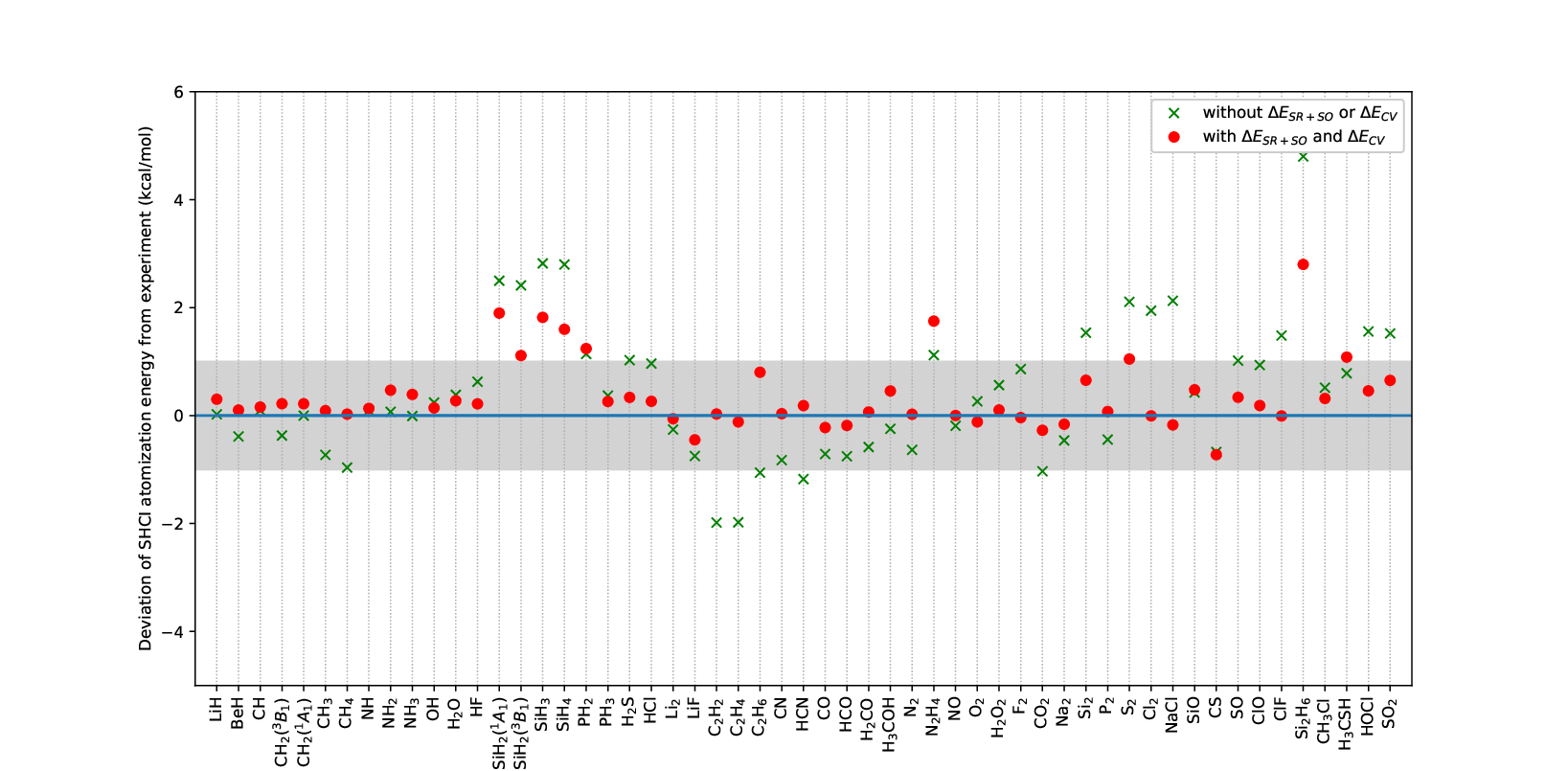
Table 1 shows the difference between the SHCI total energies for the molecules and their constituent atoms, extrapolated to the CBS limit according to Eqs. (14) and (15). It also shows the ZPE, SR+SO, and CV corrections taken from the literature and the final prediction for the SHCI atomization energy, , and how much it differs from the best available experimental values. The difference between the SHCI and experiment is also plotted in Fig. 4, both before and after the corrections are applied.
There are 3 possible sources of discrepancy between the calculated and the experimental atomization energies: (1) The extrapolation to the CBS limit may not be accurate; (2) the literature values of the ZPE, SR+SO, and CV corrections may not be accurate; 3) the experimental values have errors. It seems likely, as discussed below, that all three of these play a role for some of the systems.
We show in Fig. 5 the convergence of the atomization energies with basis size. The SHCI atomization energies in fact have two extrapolation errors. The first and more benign error comes from extrapolating SHCI total energies for each basis set to the FCI limit, i.e., . This error can be reduced by employing smaller and/or using better optimized orbitals. For the four basis sets = 2 (D), 3 (T), 4 (Q), and 5, the largest extrapolation distances in the total energy of these 55 molecules and 12 atoms are 0.97, 2.36, 3.34, and 2.90 mHa, respectively. 22 2 The extrapolation distance depends on the value of in Eq. 2 and on how well the orbitals are optimized to improve the convergence of the energy. Assuming that the extrapolated energies are in error by no more than a fifth of the extrapolation distance, all these energies should be accurate to considerably better than 1 mHa. Further, the typical extrapolation distances are much smaller, especially for the lighter systems: the median distances for the four basis sets are 2.92, 14.4, 56.4, and 77.0 Ha, respectively. The second source of error comes from extrapolation to the CBS limit, using Eqs. (14) and (15), and is less under control. For these 67 systems, the maximum and median CBS extrapolation distances are 21.8 and 6.47 mHa, respectively. This CBS extrapolation error is likely to be an important error for those systems where the extrapolation distance (the energy difference between the black dots and red crosses in Fig. 5) is large.
To further study the magnitude of the CBS extrapolation error, we add the PBE-based basis-set correction discussed in Sec. IV to the SHCI energies for each basis set [see Eqs. (IV) and (17)] and then extrapolate the corrected energies to the CBS limit according to Eq. (22), which gives us an alternative way to estimate the CBS limit of the SHCI energies. The PBE-based corrections can also be found in the Supplemental Material sup. It is apparent from Table 1 that the deviations of the SHCI and the SHCI+PBE energies from experiment are strongly correlated, thereby giving us a reasonable measure of confidence in our two extrapolations as well as an estimate of the extrapolation errors. Fig. 6 shows the same information as Fig. 5 after the PBE-based basis-set correction has been included. As summarized in Table 2, for each basis set the MAD from experiment decreases by about a factor of 3 compared to that without the basis-set correction. 33 3 To avoid confusion, we note that in Ref. Loo it was found that CCSD(T)+PBE had a MAD of only 1.96, 0.85, and 0.31 kcal/mol with respect to the CCSD(T) CBS limit for the cc-pVDZ, cc-pVTZ, and cc-pVQZ basis sets, respectively. These considerably smaller values compared to those in Table 2 are the result of a one-body basis-set correction that was always included by adding the cc-pV5Z HF energy to the CCSD(T) correlation energies for the different basis sets. Of course one could do the same for the SHCI energies in the current paper. In particular, SHCI+PBE gives a MAD of only 0.55 kcal/mol already with the cc-pVQZ basis set. The cc-pV5Z basis set has a MAD of only 0.49 kcal/mol. Applying the CBS extrapolation to SHCI+PBE gives a somewhat larger MAD from experiment of 0.51 kcal/mol, as the computed atomization energies are too small for the smaller basis sets but increase with increasing basis size and for the majority of the molecules the computed CBS atomization energies are larger than experiment.
As seen from Figs. 5 and 6 the predicted CBS atomization energy of Si2H6 is more than 3 kcal/mol larger than experiment. However, even the value is larger than experiment, so the discrepancy cannot be attributed to an inaccurate CBS extrapolation, but instead to either inaccurate ZPE, SR+SO, and CV corrections, or, to errors in the experimental value. The ZPE correction for Si2H6 is quite large, -30.50 mHa, so even a small fractional error in its estimate could account for the discrepancy in the atomization energy. In fact, these statements hold for all seven molecules in Fig. 6 that have cc-pV5Z atomization energies that are larger than experiment by more than 1 kcal/mol. Note that there are several systems for which the atomization energies are overestimated in Figs. 5 and 6 by more than 1 kcal/mol, but none for which they are underestimated by more than 1 kcal/mol.
The majority of the deviations fall below 1 kcal/mol, reaching chemical accuracy as can be seen in Table 1 and Figs. 5 and 6. As regards those where the deviations are larger than 1 kcal/mol it should also be kept in mind that that in addition to the uncertainties in the corrections, especially the ZPE correction, the experimental values may also be inaccurate, particularly for those atomization energies that are not available from the ATcT database Ruscic and Bross. For example, for PH2 the two available experimental values differ by 4.5 kcal/mol and our computed value differs by +1.5 kcal/mol from Ref. Feller and Peterson 1999 and -3.0 kcal/mol from Ref. NIS. For the molecules in the ATcT database the MAD is only 0.24 kcal/mol before the PBE-based basis set correction is applied and 0.32 kcal/mol after it is applied.
| Method | MAD | MAX |
| SHCI cc-pVDZ | 20.77 | 54.32 |
| SHCI cc-pVTZ | 6.83 | 17.43 |
| SHCI cc-pVQZ | 2.47 | 7.38 |
| SHCI cc-pV5Z | 1.20 | 3.15 |
| SHCI CBS | 0.46 | 2.80 |
| SHCI+PBE cc-pVDZ | 6.52 | 27.72 |
| SHCI+PBE cc-pVTZ | 1.47 | 6.02 |
| SHCI+PBE cc-pVQZ | 0.55 | 3.55 |
| SHCI+PBE cc-pV5Z | 0.49 | 3.36 |
| SHCI+PBE CBS | 0.51 | 3.24 |
Compared to other methods, our MAD of 0.46 kcal/mol is significantly less than the MAD of 1.2 to 3.2 kcal/mol obtained in various QMC studies Jeffrey C. Grossman 2002; Nemec et al. 2010; Petruzielo et al. 2012. Diffusion Monte Carlo works directly in the CBS limit, but the fixed-node approximation is the dominant error. Using trial wave functions with Slater determinants chosen from an SCI method, it should be easily possible to reduce considerably the fixed-node error as demonstrated in Refs. Giner et al. 2013; Giner et al. 2016; Dash et al. 2018. Our MAD is comparable to results reported from composite coupled-cluster-based methods Feller and Peterson 1999; Martin and de Oliveira 1999; Haunschild and Klopper 2012. The HEAT studies performed all-electron calculations using the coupled-cluster method with up to quadruple excitations on a somewhat different set of molecules consisting solely of first-row elementsTajti et al. 2004. Unfortunately, none of the molecules for which we have discrepancies of more than 1 kcal/mol were included. For the 19 molecules also present in the G2 set, the MAD of HEAT, SHCI, and SHCI+PBE are 0.07, 0.16, and 0.27 kcal/mol, respectively. It should be noted that HEAT is a composite quantum chemistry method, and for the lower levels of theory it employs larger basis sets than those we used, thereby significantly reducing the CBS extrapolation error.
VII Conclusion and outlook
The SHCI method enables the calculation of essentially exact energies within basis sets up to cc-pV5Z of all the molecules in the G2 set. After extrapolation to the CBS limit and addition of ZPE, SR+SO and CV corrections, the MAD from the experimental atomization energies is only about 0.5 kcal/mol. However, depending on whether we use the PBE-based basis-set corrections or not, there there are 7 or 9 molecules where the computed atomization energy is more than 1 kcal/mol larger than experiment (and none for which it is more than 1 kcal/mol smaller than experiment). These differences are mostly due to a combination of errors in the various corrections applied and in the experiments rather than lack of convergence of the SHCI energies to the FCI energies. With additional computational effort it would be possible to reduce the uncertainties in the computed energies. First, instead of adding on a CV energy correction, one could use the cc-pwCVnZ basis sets to include the correlation contribution from the core electrons. This could also make the basis-set extrapolation more reliable. Although this entails a large increase in the Hilbert space, the increase in the computational cost of the SHCI is not prohibitive because relatively few of the core excitations have a large amplitude. Second, relativistic effects could also be included within the SHCI method, as has already been demonstrated Mussard and Sharma 2018. Third, the computation of the ZPE correction would require calculating derivatives with respect to the nuclear coordinates. This could also be done, but would be the most computationally expensive part of the calculation. Fourth, the CBS extrapolation could be improved either by employing better basis sets or using a better DFT-based basis-set correction that employs the SHCI rather than the HF density matrix. With these improvements, the computed energies could be sufficiently accurate to reliably pinpoint errors in experimental values of atomization energies.
Acknowledgements.
This work was supported in part by the AFOSR under grant FA9550-18-1-0095. Y.Y. acknowledges support from the Molecular Sciences Software Institute, funded by U.S. National Science Foundation grant ACI-1547580. Some of the computations were performed at the Bridges cluster at the Pittsburgh Supercomputing Center supported by NSF grant ACI-1445606. We thank Pierre-François Loos for valuable comments on the manuscript and helping us converge the HF calculation of Si2 to the correct ground state, and one of the referees for suggesting that we use the cc-pV(+d)Z basis sets to improve the basis-set convergence.Data availability
The data that support the findings of this study are available within the article and the supplementary material of the arXiv version of this paper Yao et al..
References
- Holmes et al. (2016) A. A. Holmes, N. M. Tubman, and C. J. Umrigar, J. Chem. Theory Comput. 12, 3674 (2016).
- Sharma et al. (2017) S. Sharma, A. A. Holmes, G. Jeanmairet, A. Alavi, and C. J. Umrigar, J. Chem. Theory Comput. 13, 1595 (2017).
- Holmes et al. (2017) A. A. Holmes, C. J. Umrigar, and S. Sharma, J. Chem. Phys. 147, 164111 (2017).
- Smith et al. (2017) J. E. Smith, B. Mussard, A. A. Holmes, and S. Sharma, J. Chem. Theory Comput. 13, 5468 (2017).
- Mussard and Sharma (2018) B. Mussard and S. Sharma, J. Chem. Theory Comput. 14, 154 (2018).
- Chien et al. (2018) A. D. Chien, A. A. Holmes, M. Otten, C. J. Umrigar, S. Sharma, and P. M. Zimmerman, J. Phys. Chem. A 122, 2714 (2018).
- Li et al. (2018) J. Li, M. Otten, A. A. Holmes, S. Sharma, and C. J. Umrigar, J. Chem. Phys. 149, 214110 (2018).
- Li et al. (2020) J. Li, Y. Yao, A. Holmes, M. Otten, S. Sharma, and C. J. Umrigar, Phys. Rev. Research 2, 012015(R) (2020).
- Williams et al. (2020) K. T. Williams, Y. Yao, J. Li, L. Chen, H. Shi, M. Motta, C. Niu, U. Ray, S. Guo, R. J. Anderson, J. Li, L. N. Tran, C.-N. Yeh, B. Mussard, S. Sharma, F. Bruneval, M. van Schilfgaarde, G. H. Booth, G. K.-L. Chan, S. Zhang, E. Gull, D. Zgid, A. Millis, C. J. Umrigar, and L. K. Wagner, Phys. Rev. X 10, 011041 (2020).
- Bender and Davidson (1969) C. F. Bender and E. R. Davidson, Phys. Rev. 183, 23 (1969).
- Whitten and Hackmeyer (1969) J. L. Whitten and M. Hackmeyer, J. Chem. Phys 51, 5584 (1969).
- Huron et al. (1973) B. Huron, J. P. Malrieu, and P. Rancurel, J. Chem. Phys. 58, 5745 (1973).
- Buenker and Peyerimhoff (1974) R. J. Buenker and S. D. Peyerimhoff, Theor. Chim. Acta 35, 33 (1974).
- Evangelisti et al. (1983) S. Evangelisti, J.-P. Daudey, and J.-P. Malrieu, Chem. Phys. 75, 91 (1983).
- Giner et al. (2013) E. Giner, A. Scemama, and M. Caffarel, Can. J. Chem. 91, 879 (2013).
- Evangelista (2014) F. A. Evangelista, J. Chem. Phys. 140, 124114 (2014).
- Scemama et al. (2016) A. Scemama, T. Applencourt, E. Giner, and M. Caffarel, J. Comp. Chem. 37, 1866 (2016).
- Garniron et al. (2017) Y. Garniron, A. Scemama, P.-F. Loos, and M. Caffarel, J. Chem. Phys. 147, 034101 (2017).
- Loos et al. (2018) P.-F. Loos, A. Scemama, A. Blondel, Y. Garniron, M. Caffarel, and D. Jacquemin, J. Chem. Theory Comput. 14, 4360−4379 (2018).
- Hait et al. (2019) D. Hait, N. M. Tubman, D. S. Levine, K. B. Whaley, and M. Head-Gordon, J. Chem. Theory Comput. 15, 5370 (2019).
- Loos et al. (2020) P.-F. Loos, F. Lipparini, M. Boggio-Pasqua, A. Scemama, and D. Jacquemin, J. Chem. Theory Comput. 16, 1711 (2020).
- Curtiss et al. (1991) L. A. Curtiss, K. Raghavachari, G. W. Trucks, and J. A. Pople, J. Chem. Phys. 94, 7221 (1991).
- Curtiss et al. (2007) L. A. Curtiss, P. C. Redfern, and K. Raghavachari, J. Chem. Phys. 126, 084108 (2007).
- Feller and Peterson (1999) D. Feller and K. A. Peterson, J. Chem. Phys. 110, 8384 (1999).
- Tajti et al. (2004) A. Tajti, P. G. Szálay, A. G. Csaszar, M. Kállay, J. Gauss, E. F. Valeev, B. Flowers, J. Vázquez, and J. F. Stanton, J. Chem. Phys. 121, 11599 (2004).
- Karton et al. (2006) A. Karton, E. Rabinovich, J. M. L. Martin, and B. Ruscic, J. Chem. Phys. 125, 144108 (2006).
- Thorpe et al. (2019) J. H. Thorpe, C. A. Lopez, T. L. Nguyen, J. H. Baraban, D. H. Bross, B. Ruscic, and J. F. Stanton, J. Chem. Phys. 150, 224102 (2019).
- Jeffrey C. Grossman (2002) Jeffrey C. Grossman, Phys. Rev. Lett. 117, 1434 (2002).
- Nemec et al. (2010) N. Nemec, M. D. Towler, and R. J. Needs, J. Chem. Phys. 132, 034111 (2010).
- Petruzielo et al. (2012) F. R. Petruzielo, J. Toulouse, and C. J. Umrigar, J. Chem. Phys. 136, 124116 (2012).
- Caffarel et al. (2016) M. Caffarel, T. Applecourt, E. Giner, and A. Scemama, in Recent Progress in Quantum Monte Carlo, ACS Symposium Series, Vol. 1234 (2016) pp. 15–46.
- Dunning (1989) T. H. Dunning, J. Chem. Phys. 90, 1007 (1989).
- Giner et al. (2018) E. Giner, B. Pradines, A. Ferté, R. Assaraf, A. Savin, and J. Toulouse, J. Chem. Phys. 149, 194301 (2018).
- (34) .
- Giner et al. (2019) E. Giner, A. Scemama, J. Toulouse, and P.-F. Loos, J. Chem. Phys. 151, 144118 (2019).
- Giner et al. (2020) E. Giner, A. Scemama, P.-F. Loos, and J. Toulouse, J. Chem. Phys. 152, 174104 (2020).
- (37) Since the absolute values of for the most important determinants tends to go down as more determinants are included in the wave function, a somewhat better selection of determinants is obtained by using a larger value of in the initial iterations.
- Davidson (1989) E. R. Davidson, Comput. Phys. Commun. 53, 49 (1989).
- Epstein (1926) P. S. Epstein, Phys. Rev. 28, 695 (1926).
- Nesbet (1955) R. K. Nesbet, Proc. R. Soc. London, Ser. A. 230, 312 (1955).
- (41) S. J. Reddi, S. Kale, and S. Kumar, ICLR Published as a conference paper at the International Conference on Learning Representations, 2018.
- Helgaker et al. (1997) T. Helgaker, W. Klopper, H. Koch, and J. Noga, J. Chem. Phys. 106, 9639 (1997).
- Halkier et al. (1998) A. Halkier, T. Helgaker, P. Jørgensen, W. Klopper, H. Koch, J. Olsen, and A. K. Wilson, Chem. Phys. Lett. 286, 243 (1998).
- Halkier et al. (1999) A. Halkier, T. Helgaker, P. Jørgensen, W. Klopper, and J. Olsen, Chem. Phys. Lett. 302, 437 (1999).
- Dunning et al. (2001) T. H. Dunning, K. A. Peterson, and A. K. Wilson, J. Chem. Phys. 114, 9244 (2001).
- Wilson and Dunning (2003) A. K. Wilson and T. H. Dunning, J. Chem. Phys. 119, 11712 (2003).
- Bauschlicher Jr. and Partridge (1995) C. W. Bauschlicher Jr. and H. Partridge, Chem. Phys. Lett. 240, 533 (1995).
- Bauschlicher Jr. and Ricca (1998) C. W. Bauschlicher Jr. and A. Ricca, J. Phys. Chem. A 102, 8044 (1998).
- Perdew et al. (1996) J. P. Perdew, K. Burke, and M. Ernzerhof, Phys. Rev. Lett. 77, 3865 (1996).
- Franck et al. (2015) O. Franck, B. Mussard, E. Luppi, and J. Toulouse, J. Chem. Phys. 142, 074107 (2015).
- Sun et al. (2018) Q. Sun, T. C. Berkelbach, N. S. Blunt, G. H. Booth, S. Guo, Z. Li, J. Liu, J. D. McClain, E. R. Sayfutyarova, S. Sharma, S. Wouters, and G. K.-L. Chan, Wiley Interdisciplinary Reviews: Computational Molecular Science 8, e1340 (2018).
- Werner et al. (2012) H.-J. Werner, P. J. Knowles, G. Knizia, F. R. Manby, and M. Schütz, Wiley Interdiscip. Rev.: Comput. Mol. Sci. 2, 242 (2012).
- Garniron et al. (2019) Y. Garniron, T. Applencourt, K. Gasperich, A. Benali, A. Ferté, J. Paquier, B. Pradines, R. Assaraf, P. Reinhardt, J. Toulouse, P. Barbaresco, N. Renon, G. David, J.-P. Malrieu, M. Véril, M. Caffarel, P.-F. Loos, E. Giner, and A. Scemama, J. Chem. Theory Comput. 15, 3591 (2019).
- (54) The Supplementary Material, available at arxiv.org/src/2004.10059v2/anc, has CSV files containing geometries, HF, CCSD, CCSD(T) and SHCI energies, and, PBE-based basis set corrections.
- Feller et al. (2008) D. Feller, K. A. Peterson, and D. A. Dixon, J. Chem. Phys. 129, 204105 (2008).
- (56) B. Ruscic and D. H. Bross, Active Thermochemical Tables (ATcT) values based on ver. 1.122g of the Thermochemical Network (2019), see https://atct.anl.gov/.
- (57) B. Ruscic, A. Fernandez, J. M. L. Martin, R. E. Pinzon, D. Kodeboyina, G. von Laszewski, D. G. Archer, R. D. Chirico, M. Frenkel, and J. W. Magee, unpublished results obtained from Active Thermochemical Tables ver. 1.25 using the adjunct Thermochemical Network describing key sulfur-containing species ver. 1.056a, as reported in Ref. Karton et al. 2006.
- (58) “NIST computational chemistry comparison and benchmark database,” Release 20, August 2019, Editor: Russell D. Johnson III.
- Vasiliu et al. (2017) M. Vasiliu, K. A. Peterson, and D. A. Dixon, J. Chem. Theory Comput. 13, 649 (2017).
- Tubman et al. (2020) N. M. Tubman, C. D. Freeman, D. S. Levine, D. Hait, M. Head-Gordon, and K. B. Whaley, J. Chem. Theory Comput. 16, 2139 (2020).
- (61) The extrapolation distance depends on the value of in Eq. 2 and on how well the orbitals are optimized to improve the convergence of the energy.
- (62) To avoid confusion, we note that in Ref. \rev@citealpnumLooPraSceTouGin-JPCL-19 it was found that CCSD(T)+PBE had a MAD of only 1.96, 0.85, and 0.31 kcal/mol with respect to the CCSD(T) CBS limit for the cc-pVDZ, cc-pVTZ, and cc-pVQZ basis sets, respectively. These considerably smaller values compared to those in Table 2 are the result of a one-body basis-set correction that was always included by adding the cc-pV5Z HF energy to the CCSD(T) correlation energies for the different basis sets. Of course one could do the same for the SHCI energies in the current paper.
- Giner et al. (2016) E. Giner, R. Assaraf, and J. Toulouse, Mol. Phys. 114, 910 (2016).
- Dash et al. (2018) M. Dash, S. Moroni, A. Scemama, and C. Filippi, J. Chem. Theory Comput. 14, 4176 (2018).
- Martin and de Oliveira (1999) J. M. L. Martin and G. de Oliveira, J. Chem. Phys. 111, 1843 (1999).
- Haunschild and Klopper (2012) R. Haunschild and W. Klopper, J. Chem. Phys. 136, 164102 (2012).
- (67) Y. Yao, E. Giner, J. Li, J. Toulouse, and C. J. Umrigar, https://arxiv.org/abs/2004.10059 .