Dynamic Pricing and Mean Field Analysis for Controlling Age of Information
Abstract
Today many mobile users in various zones are invited to sense and send back real-time useful information to keep the freshness of the content updates in such zones. However, due to the sampling cost in sensing and transmission, a user may not have the incentive to contribute real-time information to help reduce the age of information (AoI). We propose dynamic pricing for each zone to offer age-dependent monetary returns and encourage users to sample information at different rates over time. This dynamic pricing design problem needs to well balance the monetary payments as rewards to users and the AoI evolution, and is challenging to solve especially under the incomplete information about users’ arrivals and their private sampling costs. After formulating the problem as a nonlinear constrained dynamic program, to avoid the curse of dimensionality, we first propose to approximate the dynamic AoI reduction as a time-average term and successfully solve the approximate dynamic pricing in closed-form. Further, we extend the AoI control from a single zone to many zones with heterogeneous user arrival rates and initial ages, where each zone cares not only its own AoI dynamics but also the average AoI of all the zones in a mean field game system to provide a holistic service. Accordingly, we propose decentralized mean field pricing for each zone to self-operate by using a mean field term to estimate the average age dynamics of all the zones, which does not even require many zones to exchange their local data with each other.
Index Terms:
Age of Information, dynamic pricing, nonlinear constrained dynamic programming, mean field gameI Introduction
Customers today prefer not to miss any useful information or breaking news even if in minute, making it imperative for a content provider to keep the posted information fresh for profit [2],[3]. The real-time information can be traffic condition, news, sales promotion, and air quality index, which will become outdated and useless over time. To keep information fresh, many content providers now invite and pay the mobile crowd including smartphone users and drivers to sample real-time information frequently [4]. Such crowdsensing approach also saves a content provider’s own cost of deploying an expensive sensor network across the city or nation. Recently, the fast development of wireless communication networks and sensors in portable devices enables the mobile users to sample and send back real-time information.
Age of information (AoI) is recently proposed as an important performance metric to quantify the freshness of the information. The literature focuses on the technological issues of the AoI such as the frequency of status updates and queueing delay analysis. In [5], the communication time of the status update systems is considered, and it proves the existence of an optimal packet generation rate at a source to keep its status as timely as possible. The Peak Age-of-Information (PAoI) metric, which is the average maximum age before a new update is received, is considered in [6] for a single-class M/M/1 queueing system. [7] shows a counter-intuitive phenomenon that zero-wait policy, i.e., a fresh update is submitted once the previous update is delivered, does not always minimize the age. Considering random packet arrivals, [8] and [9] study how to keep many customers updated over a wireless broadcast network and a Markov decision process (MDP) is formulated to find dynamic scheduling algorithms. Noting the time-varying availability of energy at the source will affect the update packet transmission rate, [10] derives an offline solution that minimizes both the time average age and the peak age for an arbitrary energy replenishment. [11] studies the jointly status sampling and updating processes that can minimize the average AoI at the destination under an average energy cost constraint for each IoT device, and shows that the optimal policy is threshold based related to the AoI state at the device and the AoI state at the destination. [12] further discusses the independent device’s waiting rate optimization in ultra-dense IoT systems by implementing mean-field games. To analytically prove the optimality of Whittle’s index policy for minimizing the AoI, [13] introduces a fluid limit model to approximate the behavior of the system and show that the performance of the policy improves as the number of users increases. For a large number of source nodes, [14] applies a mean-field approach to approximate the state distribution over the set of nodes and derives the decentralized status update policy in closed-form. [15] considers the users’ tradeoff between content update costs and their messages aging, and proposes an age threshold for the users to activate their mobile devices and update information.
However, the economic issues of controlling AoI over different zones are largely overlooked in the literature. On one hand, individuals incur sampling costs when sense and send back their real-time information to content providers, and they should be rewarded and well motivated to contribute their information updates [4]. On the other hand, recruiting a large crowdsensing pool implies a large total sampling cost to compensate, which should be taken into account in a content provider’s sustainable management of its AoI ([16], [17]). As AoI changes over time, the pricing to reward and motivate users’ sensing efforts should be dynamic and age-dependent to optimally balance the AoI evolution and the sampling cost to compensate, yet this new dynamic pricing problem is difficult to solve due to the curse of dimensionality.
Further, we face another challenge for optimally deciding the dynamic pricing in a zone: incomplete information about users’ private sampling costs and their random arrivals at the target zone to help sample. Individuals are different in nature and incur different sampling costs to reflect their heterogeneity (e.g., in battery energy consumption and privacy concern when sampling). A user will accept the price offer to sample only if his sampling cost is lower, yet the provider does not know such private cost when deciding and announcing pricing initially. In addition, users’ mobilities and their arrivals in different zones to sense are random and different.
Our key novelty and main contributions are summarized as follows.
- •
Dynamic pricing and mean field analysis for controlling AoI: To our best knowledge, this paper is the first work studying the dynamic pricing for motivating and controlling AoI update over time, and we take into account the users’ random arrivals and their hidden sampling costs. We first look at a single zone to control its individual AoI, by studying how to decide the dynamic pricing to minimize its discounted AoI and monetary payment over time. When extending to the case of many self-operated zones with heterogeneous user arrival rates and initial ages, we further study how to design the decentralized mean field pricing, where each zone cares not only its own AoI dynamics but also the average AoI of all the zones in a mean field game system.
- •
Approximate dynamic pricing for a single zone: In the nonlinear constrained dynamic pricing problem of a single zone, we propose to approximate the dynamic AoI reduction as a time-average term and successfully solve the approximate dynamic pricing in closed-form. We prove that if the current AoI is high, a high price offer should be decided to encourage many users to sample. Then we determine the time-average estimator based on Brouwer’s fixed-point theorem. We further provide the steady-state analysis for an infinite time horizon, and show that the pricing scheme (though in closed-form) can be further simplified to an -optimal version without recursive computing over time.
- •
Decentralized mean field pricing for multiple zones: For multiple zones with heterogeneous user arrival rates and initial ages, each zone should further take the average AoI of all the zones into account to provide a holistic service. To reduce the complexity of designing the dynamic pricing for many zones, we propose a mean field term to precisely estimate the average age among all the zones at each time slot. We show that the resulting decentralized dynamic pricing of each zone converges quickly, and a higher user arrival rate results in lower price. When there are a large number of zones, we prove that it is not necessary for zones to exchange their local data with each other, and the system is still ensured stable to reach almost sure asymptotic Nash equilibrium under our mean field pricing.
The rest of this paper is organized as follows. The system model and problem formulation are given in Section II. In Section III, we first look at a single zone to control its AoI and solve the approximate dynamic pricing in closed-form. Section IV provides the steady-state analysis of our approximate dynamic pricing for an infinite time horizon. The extension to many self-operated zones is studied in Section V. Section VI concludes this paper.
I-A Related Work
As discussed, the economic issues of controlling AoI in target sensing zones are largely overlooked in the literature. In the few prior works considering the AoI-economics, [16] discusses how the data providers charge the data users for each update to maximize their profits and how the data users decide their data update schedule to minimize their total costs. [17] studies two platforms’ data update schemes under negative network externality due to limited bandwidth. [18] discusses how to incentivize selfish users to provide fresh information by using fixed unit reward. In the other applications of economics and game theory, there are some related works on dynamic pricing (e.g.,[19]–[23]). For example, in [20], dynamic WiFi pricing is discussed under incomplete information of the user’s service valuation and utility type. To alleviate data congestion, time-dependent pricing is proposed in [21] for Internet service providers to time-shift users’ data demand from peak to off-peak periods. [22] considers the dynamic pricing of electricity in a retail market by finding the tradeoff between consumer surplus and retail profit. In [23], the UAV’s dynamic service pricing is analyzed by taking into consideration the UAV’s energy capacities for hovering and servicing.
However, these works don’t consider the system state evolution (e.g., the age dynamics in our problem) affected by the dynamic pricing, not to mention the mean field game framework for large population systems to provide decentralized control. Note that prior works on mean field game systems (e.g., [24]) and decentralized coordination systems (e.g., [25]) do not study the dynamic pricing for controlling the time-average state performance. In this paper, we study the dynamic pricing for controlling the weighted sum AoI and analytically solve the decentralized mean field pricing for large zone population.

II System Model and Problem Formulation
We illustrate the information update process for a single zone case in Fig. 1. The extension to multiple zones’ AoI control in a mean field game will be presented in Sections V and V-D. Here, we consider a discrete time horizon with time slot . The provider first announces price at the beginning of time slot , and a mobile user or sensor may arrive randomly in this target zone in this time slot and (if so) he further decides to sample or not by comparing the price offer and its own sampling cost . If the user appears and accepts to sample (), its sensor data (e.g., about traffic and road condition) is transmitted with random transmission delay to reach the provider’s app for end-customers to access.
We consider that the users (e.g., drivers in a traffic flow) arrive in each zone according to a Poisson process as in the related literature (e.g., [26] and [27]) with average number of user arrivals per unit time . Then, the probability of the random number of user arrivals in the -th time slot of interval being equal to is with small enough duration for each time slot. Note that becomes trivial as long as we set small. Thus, each time slot’s duration is properly selected to be short such that it is almost sure to have at most one user arrival at a time.11 1 For multi-zone case in Section V, to ensure at most one user arrival in a time slot for every zone, the time duration is chosen by , where is the time duration that at most one user arrive in a time slot for zone . As shown in Fig. 1, if a user arrives in time slot , ; otherwise, , with the user arrival rate in each time slot . Further, the users’ sampling costs are i.i.d. according to a cumulative distribution function (CDF) , where upperbound is estimated from historical data. Though all potential users’ costs follow the same distribution, their realized costs are different in general. Under the incomplete information, the provider does not know the users’ arrivals for potential sampling at time or the arriving user’s particular cost . It only knows the user arrival probability in each time slot and the cost distribution . In this paper, we consider non-trivial user arrival rate and small transmission delay . Otherwise, the provider should always set the price to be the upperbound to encourage the rarely arriving users to sample and reduce the AoI.

We adopt the Age of Information (AoI) as the performance metric to quantify the freshness of the information packet at end-customer side. Let be the instantaneous or realized AoI at the beginning of time slot . Considering a linearly increasing actual age model as in Fig. 2 for the discrete time horizon with age increasement of each time slot normalized to one time slot duration, the new age at time increases from to , if the information is not sampled by any user at time . If a user arrives at time , i.e., , and further accepts the price , i.e., , a new status packet will be generated and transmitted. Then, the new age at time drops to by noting the small transmission delay (e.g., in milliseconds) due to small data size of real-time information (e.g., traffic speed). Without loss of generality, we assume the status sampling and transmission are accomplished within a time slot [28].22 2 This is reasonable as the information sampling plus transmission delay (in milliseconds) is not comparable to each time slot’s duration (in seconds or minutes), and the latter time scale is used to model a new user’s physical arrival in the zone. Then, the dynamics of the instantaneous AoI is given as
| (1) |
As long as follows the i.i.d. distribution over any time slot, we denote as the expected transmission delay of a new data sample. Denote as the conditional probability to incur AoI at time , given price is applied under instantaneous AoI at time . According to (1), given the CDF of an arriving user’s cost , the conditional probability that the AoI at time will reduce to is ; and the conditional probability that the AoI at time will increase to is . Therefore, the expected AoI at time is
| (2) |
For ease of reading, we rewrite the conditional expectation in (II) as . Considering uniform distribution for the users’ private costs (i.e., , ), according to (II), the dynamics of the expected age to next time is given as:
| (3) |
which shows nonlinear AoI evolution due to the product of the expected age and in the second term above.
Since the probability that a user appears and accepts the price is , the expected payment to this user is . Note that the optimal price should not exceed the maximum cost of the user as it is unnecessary for the provider to over-pay. The objective of the provider is to determine the optimal dynamic pricing that minimizes the expected total discounted cost over time, which is the summation of the square expected age and expected monetary payment over time:
| (4) |
where is the discount factor and indicates the provider values the current costs than that of future. We choose the typical square expected age as in many economics papers [29] to reflect the fact that the platform provider’s profit loss should be convexly increasing in the age of its provided information.33 3 The end-customers are sensitive to information freshness and many media platforms (e.g., Netflix, navigation apps) want to keep provided information as fresh as possible. If the AoI is large, the user experience is bad due to outdated information and the end-customers may switch to other providers, which leads to profit loss.
The problem in (II)-(4) is a nonlinear constrained dynamic program, which is challenging to solve analytically due to the curse of dimensionality. Imagining that a huge number of time-dependent prices must be jointly designed with the price interval , then the computation complexity is formidably high and increases exponentially in . To analytically solve this problem for useful insights and guidelines to the provider, we will propose an approximation of dynamic pricing in the following section.
III Approximation of Dynamic Pricing
To analytically obtain the optimal dynamic prices for the nonlinear constrained dynamic problem in (II)-(4), we approximate the nonlinear dynamics constraint of the expected age in (II) into linear dynamics. Specifically, we propose a time-average term as an estimator to approximate the possible age reduction at each time slot in (II), i.e.,
| (5) |
Here, the time-average estimator is viewed as the time-average age reduction of each time slot and its estimation should also take into account the time discount factor , i.e.,44 4 There is no need to include in estimation, as it will not affect the AoI in any previous time slot .
| (6) |
Note that when time discount factor , by applying L’Hôpital’s rule, we have .
In the following, given any estimator , we analyze the approximate dynamic pricing in Section III-A. Later in Section III-B, we will further analyze how to determine the estimator for finalizing pricing update. We will also show that this approximate dynamic pricing approaches the optimal dynamic pricing well.
III-A Analysis of Approximate Dynamic Pricing
Though the dynamic programming problem (4)-(5) now has only linear AoI evolution constraint in (5), it is still not easy to solve by considering the huge number of price combinations over time. We denote the cost objective function from initial time as
| (7) |
and the value function given the initial age as
| (8) |
Then, we have the dynamic programming equation at time :
| (9) |
s.t. (5)


In the following, we will analyze the optimal solution to the dynamic problem above by using dynamic control techniques.
Proposition III.1
The approximate dynamic pricing as the optimal solution to the dynamic program (4)-(5) is monotonically increasing in and given by55 5 Note that (10) automatically satisfies the constraint as long as the transmission delay is not huge and the zone has non-trivial user arrival rate . In extreme case of for the first few time slots (e.g., due to huge initial age ), we can simply reset to be the upperbound and expected age will decrease and ensure in the long run.
| (10) |
with , and the resulting expected age at time is
| (11) |
where
| (12) |
| (13) |
with on the boundary.
Proof Sketch: According to the first-order condition when solving (9) in the backward induction process, we notice that is a linear function of . Thus, the value function in (9) should follow the following quadratic structure with respect to :
| (14) |
yet we still need to determine . This will be accomplished by finding the recursion in the following.
First, we have on the boundary due to . Given as in (14), the dynamic programming equation at time is
| (15) |
Substitute in (5) into (15) and let , we obtain the optimal price in (10). Then, we substitute in (10) into in (15), and obtain as a function of and . Finally, by reformulating in (15) and noting that , we obtain the recursive functions of and in (12) and (13). Substitute in (10) into (5), we obtain the expected age in (11).
Note that in (10) also applies to the case without discount factor (i.e., ) and we expect a less myopic pricing to control future age increment. Fig. 3 simulates the system dynamics over time under the approximate dynamic price in (10). We can see that when the initial age is low, is low initially to save sampling cost and can allow the age to increase mildly. The price then increases with the increased age until both of them reach steady-states. This is consistent with the monotonically increasing relationship between and in (10). Yet when close to the end of the time horizon , the price decreases to to save immediate sampling expense without worrying its effect to increase the future age. Consequently, the expected age increases again but only lasts for a few time slots.
III-B Update of Estimator for Finalizing Pricing
Now we are ready to update the estimator defined in (6) for finalizing dynamic pricing in (10). The estimator is affected by all the estimated ages over the time horizon , which will in turn affect in (11) in the closed loop. Thus we next determine by finding the fixed point of (6), which will be shown to exist in our problem.

For any , we substitute in (6) into in (11), and define
| (16) |
which tells is a function of all the ages . Then, we summarize by using the following vector function for :
| (17) |
The fixed point (if any) in should be reached to let replicate in (6) in the first place.
Note that in (12) and in (13), we have the following upperbound for (16):
| (18) |
Define continuous space in dimensions. Since each in (16) is continuous in , the vector function in (17) is a continuous mapping from to . According to the Brouwer’s fixed-point theorem, we have the following proposition.
Proposition III.2
in (17) has a fixed point in .
Given the existence of the fixed point, we are ready to find the estimator in (6). Accordingly, we propose Algorithm 1: given any initial estimator in round , we can iteratively obtain the resulting expected ages according to (11), and then check whether the resulting estimator in next round converges to the last-round estimator . By repeating the iteration process until is in the neighborhood of with error , we obtain the fixed point and the computation complexity of Algorithm 1 is . As shown in Fig. 4, converges to the fixed point within iterations. After obtaining the value of along with and , we just need to substitute them into the closed-form solution in (10) and obtain approximate dynamic pricing.


In the following, we examine the performance of the approximate dynamic pricing in (10) in the original AoI dynamics system (II) without linearizing the age reduction in (5). We wonder if the approximate pricing obtained after linearization still ensures the expected age in the original AoI dynamics to converge and reach a steady-state. If so, we want to further examine the performance gap between the total expected costs under the optimal dynamic price (obtained via exhaustive search) and our approximate dynamic price in the original system.
First, by applying the approximate dynamic pricing in (10) to the original AoI dynamics in (II), Fig. 5 shows that the expected age still converges to a steady-state only after a few time slots, which shows that our approximate pricing is feasible to control the AoI evolution in the original system. This figure is similar to Fig. 3(b) in the linearized AoI dynamics system (under the same parameter setting). Thus, we can tell that the time-average estimator approximates the age evolution well.
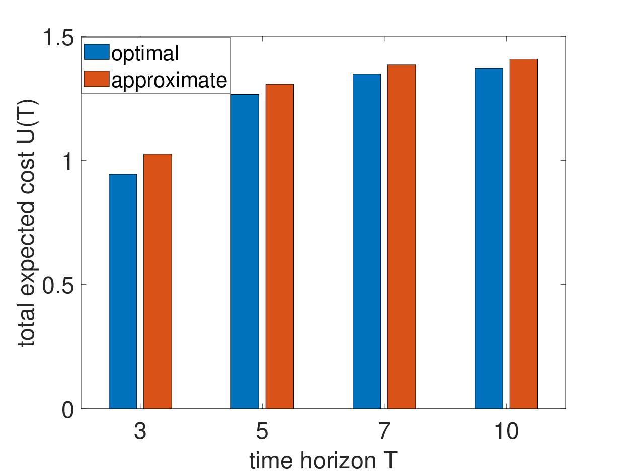
Although we may imagine that the approximate dynamic pricing will cause performance losses (though saving computational complexity greatly), Fig. 6 shows that the total expected cost gap between the optimal dynamic pricing and our approximate dynamic pricing in the original system (II)-(4) is small.
III-C Extension to Other Distributions of Users’ Private Costs

Our results can also be extended to some other continuous distributions of users’ private costs with CDF function by applying the first-order approximation on . To be specific, we first use a linear function to approximate , where and are coefficients returned by linear regression. Take the truncated normal distribution for example, it has original CDF:
| (19) |
with mean and variance . As shown in Fig. 7, we approximate it as the linear function , which is truncated within .
Then, based on the linear approximation , similar to our analysis in Sections III-A and III-B, we can obtain the approximate dynamic pricing as in (10). It is shown in Fig. 8 that, for the truncated normal distribution of users’ private costs, the total expected cost gap between the optimal dynamic pricing (obtained via exhaustive search with original CDF in (19)) and our approximate dynamic pricing in (10) (with the first-order approximation of the CDF ) in the original nonlinear system is small.
IV Steady-state Analysis of Dynamic Pricing


We wonder how our approximate dynamic pricing and its performance would be in the steady-state, by looking at the infinite time horizon in this section. As , there is no ending time and we do not observe the surge of pricing and age as in Figs. 3 and 5 when closing to the end . We will show that the approximate dynamic pricing can be further simplified to an -optimal version without recursive computing in (10) over time. Specifically, the steady-state characterizations of in (12) and in (13) can be found by iterating the dynamic equations until they converge. The following lemma shows the steady-states of and , both of which exist and are nicely given in closed-form.
Proof: Starting from the boundary condition , according to in (12) and in (13), we can obtain and backward given and at next time slot. Rewrite above as
| (22) |
Starting from and note that , we have . Note that (22) is increasing with and , we can conclude that is bounded increasing sequence in the reverse time order and will converge to the steady-state , which can be solved as (IV.1) by removing the time subscripts from (12).

By removing the time subscripts from (13), the steady-state is solved as in (21). In the following, we will show that is bounded increasing sequence in the reverse time order and converges to . According to in (13), define as the right-hand side of (13) given the steady-state , i.e.,
| (23) |
Take the derivative of with respect to , we have
| (24) |
According to , we have . Thus, and increases with . Since is an increasing sequence and converges to , .
Starting from , we have . Since increases with , as shown in Fig. 11, the equation set intersects with the vertical axis with . The slope of each equation satisfies . Therefore, starting from , we have based on . Then, from , we have based on . Thus, we can obtain until .
Figs. 9 and 10 simulate the dynamics of in (12) and in (13). We can see that both and fast converge to their steady-states in a few rounds.
Proposition IV.1
For the infinite time horizon case, the approximate pricing is simplified from (10) to
| (25) |
and the resulting expected age at time is
| (26) |
As , the expected age converge to
| (27) |
and the optimal dynamic pricing converges to
| (28) |
In the following, we prove the existence and uniqueness of the fixed point estimator for the infinite time horizon.
Proposition IV.2
For the infinite time horizon, the estimator exists and can be solved as the unique positive solution to the following equation:
| (29) |
where in (IV.1) is a function of .
Proof: Note that is estimated by in (6). Since converges to (27), as , we can further estimate as
| (30) |
It is easy to check that and above increase with . Thus, increases with . Note that is close to for small delay , and . Since the right-hand side of (29) is a constant, the positive fixed point is the unique solution to (29).
IV-A -optimality for the Simplified Pricing in (25)
We note that the approximate dynamic pricing is further simplified to (25) by using the steady-states in (IV.1) and in (21) for infinite time horizon. It is unlike (10) which still recursively updates in (12) and in (13) for updating in finite horizon case. By using this simple dynamic price without recursive computing over time, we wonder its performance for a finite horizon and denote the resulting expected discounted cost objective as . In the following proposition, we prove that under simplified approximate dynamic pricing in (25) is -optimal compared with the expected discounted cost in (4) under approximate dynamic pricing in (10).
Proposition IV.3
, there always exists an such that
| (31) |
and we have for a sufficiently large horizon .
Proof: Since and converge to the steady-states and respectively in the reverse time order, there exists a time threshold ( time slots before the end of time horizon ) such that for any , and . Then, for any , we have in (IV.1). Moreover, according to (10) and (25), we have for any . Therefore, the expected discounted cost in (4) under (10) can be rewritten as
| (32) |
where .
Given the fixed threshold time slots before the end of the time horizon , according to (33) and (34), we have and . Thus, we have
| (35) |
Similarly, we can show that . Since in (10) is optimal for finite horizon, we have . Combine (IV-A) and (IV-A), we have , and thus for , there always exists a such that with .

As shown in Fig. 12, we numerically show the difference between and reduces as increases, which approaches for sufficiently large . This is consistent with this proposition above and tells that the simple pricing in (25) performs well once is large (e.g., in this numerical example and is not necessarily infinite). In addition, Fig. 12 also shows that the convergence rate of (25) to approach (10) decreases with the discounted factor . This is because as increases, the impact of the ages and prices of further time slots on the total cost objective would increase, which will result in greater cost gap.
V Decentralized Pricing and Mean Field Analysis for Multi-zone AoI System
In this section, we extend the AoI control from a single zone to many self-operated zones who coordinate to provide the same type of information service (e.g., live traffic guidance) to end-customers. In reality, there are a large number of zones in a city to update the information (e.g., traffic road information), and the users arriving in each zone are invited to sense and send back real-time information to keep the overall information fresh. Due to the heterogeneity of the zones (e.g., downtown or suburban areas), we practically consider that their user arrival rates and initial AoI are different.
V-A Modelling of Multi-zone AoI System
More specifically, we consider zones with heterogenous user arrival rates and initial ages , and they self-operate to decide pricing incentives locally and control their own AoI dynamics. In reality, the user arrival rates of neighboring zones may be correlated. Denote the joint probability mass function of users’ arrivals in zone and other zones as , where , indicates the user’s arrival in time slot and otherwise. As users’ random arrivals over time in each zone are identical distributed, for each zone , its user arrival rate is given by its marginal probability . For example, if there are two zones and and their user arrival rates are closely related in the joint probability of users’ arrivals in both zones. Given and , the user arrival rate of zone is updated to . As end-customers are moving and may travel across various zones, each self-operated zone not only needs to care about the AoI within its own zone but also the other zones’ information freshness to ensure overall service experience to end-customers [30]. For example, Waze and Waycare share their traffic data sampled in different zones to provide the same type of live guidance service and guide the drivers to travel between different zones [31].
In this new multi-zone self-operated system, each zone should consider a weighted sum AoI consisting of its own age and the average age of all the zones, i.e., with zone ’s weight . A special case of this model is where each zone is not cooperative at all and only cares about its own AoI. As studied in Sections III and IV, then the system operation simply degenerates to independent operation by each zone, and our dynamic pricing schemes in Propositions III.1 and IV.1 for each zone can be applied. In the general model with in this section, however, the average information age across all the zones exhibits network externality and makes the multi-zone joint pricing design over time and zone (space) more challenging here.
Note that the weighted sum AoI of each zone is affected by all the other zones’ AoI and their corresponding dynamic pricing. Different from (II)-(4), the objective of each zone is to choose its optimal dynamic pricing as the best response to and minimize its expected discounted cost, i.e.,
| (37) |
| (38) |
where are different due to different user arrival rates and initial ages in different zones. Only when , the multi-zone decentralized pricing problem degenerates to the single zone problem in (II)-(4).
Similar to the analysis method in Section III, we first transform the nonlinear dynamics of the expected age in (38) to linear dynamics, by introducing a time-average estimator for zone . That is, the AoI dynamics in (38) changes to
| (39) |
where the time-average term is estimated in the following way as in (6):
| (40) |
Note that is different for different zones and is affected by all the zones’ user arrival rates and ages , over time due to the multi-zone coupling of weighted sum AoI in the objective (37).
V-B Analysis of Decentralized Mean Field Pricing
In this section, we first propose mean-field term to approximate the average age dynamics of all the zones for the ease of operation at individual zones, and then analyze the decentralized mean-field pricing for each zone given any mean-field term and any zone’s time-average estimator. Later in Section V-C, we will further analyze how to determine the mean field term and time-average estimators for finalizing pricing update.
Regarding the minimization of the discounted cost function in (37), the dynamic pricing design of each zone must take into account the average age of all the zones. In practice, it is not easy for each zone to keep tracking AoI dynamics of many other zones for adapting its own pricing due to large communication overhead. To make the AoI control of each self-operated zone easy to implement in practice, we desire a decentralized dynamic pricing without requiring all the zones to exchange information with each other from time to time. Therefore, we propose the following mean field term which should satisfy
| (41) |
to estimate the average information age over time. Then each zone aims to design the decentralized mean field pricing according to for minimizing its estimated total discounted cost. The problem changes from (37)-(38) to the following:
| (42) |
s.t. (39)
Given any mean-field term in (41) and any zone ’s time-average estimator in (40), we can analyze the decentralized mean field pricing scheme for the dynamic system in (39) and (V-B), by using the similar method as in Proposition III.1.
Proposition V.1
In the dynamic system in (39) and (V-B), the optimal decentralized mean field pricing of zone at time is
| (43) |
with , and in (V.1) is a function of mean field term , which is affected by AoI of all the other zones. The resulting expected age at time is
| (44) |
where is a function of , and are obtained recursively:
| (45) |
| (46) |
with .
We can see that, different from Proposition III.1 for a single zone, here in (V.1) depends on the mean field term and the weight of zone . Notice that the dynamic pricing of zone will affect and thus . Thus, will also affect the age of any other zone via .
V-C Update of Mean Field Term and Time-average Estimators for Finalizing Pricing
Given the optimal decentralized pricing in (V.1), we are ready to determine the mean field term and time-average estimators . Note that the estimators to estimate the dynamic age reduction of zone and to estimate the average age are affected by in (V.1) of all the zones over time, which will in turn affect the age of each zone at time . Given the user arrival rates and initial ages of all the zones, we next determine and by finding the fixed points of (40) and (41), respectively.
Proposition V.2
Proof: For any zone , substitute and into in (V.1), we can see that the age of zone at time is a function of the ages of all the zones over time. Define the following function as a mapping from to zone ’s age in (33) at time :
| (47) |
To summarize any possible mapping in (47), we can define the following vector function as a mapping from to the set of all the zones’ ages over time:
| (48) |
Thus, the fixed point to in (V-C) should be reached to let and replicate and , respectively.
We can check that . Define set . Since is continuous, is a continuous mapping from to . According to the Brouwer’s fixed-point theorem, has a fixed point in .


Let us explain the procedure of Algorithm 2 in the following. Given any initial estimators and in round , we iteratively obtain the resulting expected ages for each zone according to (V.1). By repeating the iteration process until and within arbitrarily small error , the computation complexity of Algorithm 2 is . Different from Algorithm 1 for searching only in the time domain, here Algorithm 2 jointly searches through both time and zone domains. As shown in Figs. 13 and 14, the local estimator of each zone and mean field estimator of each time slot converge to the fixed point and within iterations, respectively.
In the simulations, by applying the decentralized mean field pricing in (V.1) to the original nonlinear system (38), we first consider zones with identical initial age and weight , and choose varying user arrival rate to show the impact of user arrival rates on the mean field pricing. As shown in Fig. 15, the mean field pricing of each zone converges to a steady-state fast (within time slots), and a higher user arrival rate motivates this zone to set a lower mean field pricing as compared to the other zones. This is because the zone can patiently wait for a target user with low sampling cost if there are more user arrivals to sample. When close to the end of the time horizon , the price decreases to to save immediate sampling expense without worrying the future age.


In another simulation, we examine the convergence of the expected age by applying in (V.1) to the original nonlinear AoI dynamics (38). As shown in Fig. 16, for heterogeneous zones with different user arrival rates , initial ages and weight , , the expected age of each zone converges to a steady-state quickly. When close to the end of the time horizon , the expected age increases again due to decreasing to the end. Fig. 16 also shows that our mean field term approximates well to the average age under original AoI dynamics (38).
V-D Decentralized Pricing and Mean Field Term Estimation using Large Population Limit
Our mean field term estimation in Algorithm 2 require each zone to know any other zone ’s local data, i.e., initial age and user arrival rate . Such local data are not constant all the time but change over different time periods (e.g., from off-peak to peak hours). Even each zone manages to collect such data over time, yet such local data sharing among a large number of zones (in a metropolis) introduces a large of communication overhead. In this section, we want to extend the decentralized solution developed in last section using large population limit.
We propose to employ the large population limit to determine the joint empirical distribution of the arrival rates and initial ages, and then predict the mean field term accordingly. To be specific, when the zone population is sufficiently large, the arrival rate and initial age of any individual zone no longer play important roles. We care about the occurrence frequency of any possible value and any value in the respective feasible sets and to determine the age evolution as well as the mean field term . Define the joint empirical CDF of the zones for the two dimensional sequences with feasible sets and as:
| (49) |
Then, according to the joint empirical CDF , we have
| (50) |
where is the expected age of a typical zone at time with arrival rate and initial age .
Suppose there exists a continuous CDF with such that as widely adopted in large population models [24], [32]. Since we want the mean field term to replicate and we only know the joint cumulative distribution instead of realized and , we employ the large population limit to estimate , i.e.,
| (51) |
Then, for any given mean field estimator in (51), we can obtain the decentralized dynamic pricing in (V.1) and expected age in (V.1) as in Proposition V.1. Given the joint cumulative distribution , we can also determine the fixed point mean field estimator according to Algorithm 2, by replacing in Line of Algorithm 2 with
| (52) |
Here, we should note that in Algorithm 2, and calculated according to (45) and (V.1) are functions of , and thus the resulting age is a function of and .
In the following proposition, we show that the mean field term introduced in (51) is a perfect estimator of the average age , as long as the zone population is sufficiently large.

Proof: In the following proof, we first consider the one dimensional case by fixing the initial ages of all the zones to be the same. Then, the mean field term in (51) can be simplified as
| (54) |
where is the expected age of the zone at time with user arrival rate .
Then, we extend the domain of from to in order to use Helly-Bray Theorem. Assume . Define
| (56) |
Thus, we have extended function to with and . Since in (45) and in (V.1) are continuous in , and the denominators of in (V.1) are positive, is continuous in . Note that is bounded, according to Helly-Bray Theorem, if converges weakly to ,
| (57) |
Thus,
| (58) |
We can extend this result similarly in the two dimension case with both heterogeneous initial ages and user arrival rates.
V-D1 Almost Sure Asymptotic Nash Equilibrium
In the following, we will analyze the performance of the decentralized mean field pricing in (V.1), which is designed based on the mean field estimator without requiring each zone to know the other zones’ initial ages and user arrival rates. Note that such lack of information may disrupt the decentralized mean field pricing and hinder the multi-zone self-operated system to converge to a stable state. Thus, our main concern here is whether the decentralized mean field pricing scheme in (V.1) (with in (51) locally estimated by each zone) ensures system stability to reach almost sure asymptotic Nash equilibrium.
Definition V.1
A set of dynamic pricing with is called an almost sure asymptotic Nash equilibrium with respect to the total expected cost objective in (37), if there exists a sequence of non-negative variables such that for any ,
where .
We next prove that the system stability is ensured by our decentralized pricing in (V.1) and in (51).
Proposition V.4
Proof: For any , we have
| (61) |
By the Cauchy-Schwarz inequality, we have
| (62) |
Since is bounded due to bounded , and thus .
Note that is the optimal solution with respect to the estimated discounted cost function in (V-B), i.e., . Then, similar to the above analysis, we have
| (63) |
Based on Proposition V.3, for any , . Therefore, we have .
VI Conclusion
In this paper, we have studied the AoI control by using dynamic pricing to well balance the AoI evolution and monetary payments over time. We have formulated this problem as a nonlinear constrained dynamic program under the incomplete information about users’ random arrivals and their private sampling costs. To avoid the curse of dimensionality, we first propose a weighted time-average term to estimate the dynamic AoI reduction, and successfully solve the approximate dynamic pricing in closed-form. We further provide the steady-state analysis for an infinite time horizon, and show that the pricing scheme (though in closed-form) can be further simplified to an -optimal version without recursive computing over time. Finally, we extend the AoI control from a single zone to many zones with heterogeneous user arrival rates and initial ages, where each zone cares not only its own AoI dynamics but also the average AoI of all the zones to provide a holistic service. Accordingly, we design decentralized mean field pricing for each zone to self-operate by using a mean field term to estimate the average age dynamics of all the zones, which does not even require many zones to exchange their local data with each other.
References
- [1] X. Wang and L. Duan, “Dynamic pricing for controlling age of information,” in IEEE International Symposium on Information Theory (ISIT), 2019.
- [2] D. Guan, “Five industries that should take a cue from Netflix and crowdsource parts of its tech,” TechCrunch, 2016.
- [3] T. NewsDesk, Google Improves Maps Data With New Crowdsourcing Features, 2016.
- [4] L. Duan, T. Kubo, K. Sugiyama, J. Huang, T. Hasegawa, and J. Walrand, “Motivating smartphone collaboration in data acquisition and distributed computing,” in IEEE Transactions on Mobile Computing, 2014.
- [5] S. Kaul, R. Yates, and M. Gruteser, “Real-time status: How often should one update?” in Proceedings of IEEE INFOCOM, 2012.
- [6] M. Costa, M. Codreanu, and A. Ephremides, “Age of information with packet management,” in IEEE International Symposium on Information Theory (ISIT), 2014.
- [7] Y. Sun, E. Uysal-Biyikoglu, R. D. Yates, C. E. Koksal, and N. B. Shroff, “Update or wait: How to keep your data fresh,” IEEE Transactions on Information Theory, vol. 63, no. 11, pp. 7492–7508, 2017.
- [8] Y.-P. Hsu, E. Modiano, and L. Duan, “Age of information: Design and analysis of optimal scheduling algorithms,” in IEEE International Symposium on Information Theory (ISIT), 2017.
- [9] ——, “Scheduling algorithms for minimizing age of information in wireless broadcast networks with random arrivals,” IEEE Transactions on Mobile Computing, forthcoming, 2019.
- [10] B. T. Bacinoglu, E. T. Ceran, and E. Uysal-Biyikoglu, “Age of information under energy replenishment constraints,” in IEEE Information Theory and Applications Workshop (ITA), 2015.
- [11] B. Zhou and W. Saad, “Joint status sampling and updating for minimizing age of information in the internet of things,” IEEE Transactions on Communications, vol. 67, no. 11, pp. 7468–7482, 2019.
- [12] ——, “Age of information in ultra-dense iot systems: Performance and mean-field game analysis,” arXiv preprint arXiv:2006.15756, 2020.
- [13] A. Maatouk, S. Kriouile, M. Assaad, and A. Ephremides, “On the optimality of the whittles index policy for minimizing the age of information,” IEEE Transactions on Wireless Communications, 2020.
- [14] Z. Jiang, S. Zhou, Z. Niu, and C. Yu, “A unified sampling and scheduling approach for status update in multiaccess wireless networks,” in IEEE INFOCOM 2019-IEEE Conference on Computer Communications. IEEE, 2019, pp. 208–216.
- [15] E. Altman, R. El-Azouzi, D. S. Menasche, and Y. Xu, “Forever young: Aging control for hybrid networks,” in Proceedings of the Twentieth ACM International Symposium on Mobile Ad Hoc Networking and Computing (MobiHoc), 2019, pp. 91–100.
- [16] M. Zhang, A. Arafa, J. Huang, and H. V. Poor, “How to price fresh data,” in The International Symposium on Modeling and Optimization in Mobile, Ad Hoc, and Wireless Networks (WiOpt), 2019.
- [17] S. Hao and L. Duan, “Regulating competition in age of information under network externalities,” IEEE Journal on Selected Areas in Communications, 2020.
- [18] B. Li and J. Liu, “Can we achieve fresh information with selfish users in mobile crowd-learning?” in 2019 International Symposium on Modeling and Optimization in Mobile, Ad Hoc, and Wireless Networks (WiOPT). IEEE, 2019, pp. 1–8.
- [19] A. Gershkov and B. Moldovanu, Dynamic Allocation and Pricing: A Mechanism Design Approach. MIT Press, 2014, vol. 9.
- [20] J. Musacchio and J. Walrand, “Wifi access point pricing as a dynamic game,” IEEE/ACM Transactions on Networking, vol. 14, no. 2, pp. 289–301, 2006.
- [21] S. Sen, C. Joe-Wong, S. Ha, and M. Chiang, “Incentivizing time-shifting of data: A survey of time-dependent pricing for internet access,” IEEE Communications Magazine, vol. 50, no. 11, pp. 91–99, 2012.
- [22] L. Jia and L. Tong, “Dynamic pricing and distributed energy management for demand response,” IEEE Transactions on Smart Grid, vol. 7, no. 2, pp. 1128–1136, 2016.
- [23] X. Wang and L. Duan, “Dynamic pricing and capacity allocation of uav-provided mobile services,” in IEEE International Conference on Computer Communications (INFOCOM), 2019, pp. 1855–1863.
- [24] M. Huang, P. E. Caines, and R. P. Malhamé, “Large-population cost-coupled LQG problems with nonuniform agents: individual-mass behavior and decentralized -Nash equilibria,” IEEE transactions on automatic control, vol. 52, no. 9, pp. 1560–1571, 2007.
- [25] Y. Guo, M. Pan, Y. Fang, and P. P. Khargonekar, “Decentralized coordination of energy utilization for residential households in the smart grid,” IEEE transactions on smart grid, vol. 4, no. 3, pp. 1341–1350, 2013.
- [26] B. D. Greenshields, D. Schapiro, and E. L. Ericksen, Traffic performance at urban street intersections, 1946.
- [27] D. L. Gerlough and A. Schuhl, Use of Poisson distribution in highway traffic. Eno Foundation for Highway Traffic Control Saugatuck, Conn., 1955.
- [28] ETSI, “Why do we need 5G,” https://www.etsi.org/technologies/5G.
- [29] S. Wang, “Microeconomic Theory,” Springer Texts in Business and Economics, Springer, 2018.
- [30] Y. Li, C. A. Courcoubetis, and L. Duan, “Dynamic routing for social information sharing,” IEEE Journal on Selected Areas in Communications, vol. 35, no. 3, pp. 571–585, 2017.
- [31] C. Shu, “Waze signs data-sharing deal with ai-based traffic management startup waycare,” TechCrunch, 2018.
- [32] M. Huang, R. P. Malhamé, and P. E. Caines, “Nash equilibria for large-population linear stochastic systems of weakly coupled agents,” Analysis, control and optimization of complex dynamic systems, pp. 215–252, Springer, 2005.