Characterization of the umbra–penumbra boundary by the vertical component of the magnetic field

For this study, 11 data sets of fully-fledged sunspots were selected from the GRIS archive ¹¹ 1 sdc.leibniz-kis.de, where observations since 2014 are publicly available. The GRIS instrument (Collados et al. 2012) is a slit-spectograph in the infrared regime providing high resolution spectropolarimetric data. It is attached to the 1.5 m GREGOR telescope situated at the Observatorio del Teide, Tenerife (Schmidt et al. 2012); the telescope is equipped with an adaptive optics system (Berkefeld et al. 2012).
The selection criteria used to obtain our samples of sunspots were that a) the Fe I $15\,648\text{\,}\mathrm{\SIUnitSymbolAngstrom}$ and the $15\,662\text{\,}\mathrm{\SIUnitSymbolAngstrom}$ line were recorded simultaneously, b) the sunspot contained a fully-fledged penumbra, c) the heliocentric angle was not larger than $35\text{\,}\mathrm{\SIUnitSymbolDegree}$, and d) the data quality (especially seeing) was sufficient. In Table 1, a list of these data sets is shown. The recorded spectral windows were approximately $40\text{\,}\mathrm{\SIUnitSymbolAngstrom}$ wide, with central positions that differed only slightly. The wavelength pixel size was $\delta_{\lambda}\approx$0.04\text{\,}\mathrm{\SIUnitSymbolAngstrom}$$ and the spatial pixel size, as obtained from a correlation with HMI data (Borrero et al. 2016), was $\delta_{xy}\approx$0.135\text{\,}\mathrm{\SIUnitSymbolArcsecond}$$. The data was demodulated and corrected with the standard GRIS pipelines (see Franz et al. 2016, for a description of some of the included methods) and we worked with the data cubes from the level 2 data, which includes a wavelength calibration and the derivation of the spot coordinates based on HMI images. In addition, we corrected for the daily variations of solar flux (creating an intensity gradient for subsequent slit positions) with a linear fit over the scanning direction.

The SIR inversion code (Ruiz Cobo & del Toro Iniesta 1992) offers the possibility of providing a spatial straylight profile $\mathbf{I_{\mathrm{stray}}}$ for each pixel:

Using Eq. 1, this straylight profile is added to the full-Stokes synthetic profile $\mathbf{I^{*}}$ of the respective atmosphere before the fit is compared to the actual observed full-Stokes profile $\mathbf{I_{\mathrm{obs}}}$. We calculated a specific full-Stokes spatial straylight profile for each pixel separately. Following the idea by Borrero et al. 2016, we calculated the straylight profile as the sum over all pixels of the map. However, each pixel was weighted with a two-dimensional Gaussian centered at the respective pixel, so that neighboring pixels contribute more. The full width at half maximum (FWHM) of this Gaussian was $47.1\text{\,}\mathrm{\SIUnitSymbolArcsecond}$ (equivalent to a standard deviation of $\sigma=$20\text{\,}\mathrm{\SIUnitSymbolArcsecond}$$), as estimated by Borrero et al. 2016. The advantage of a local straylight profile is that, in addition to intensity straylight profiles, meaningful Stokes Q, U, and V straylight profiles can be obtained. Neighboring pixels are assumed to have a more similar polarization signal than far-away pixels, and therefore cancellation effects in Q, U, and V are less probable.
The factor $\alpha$ in Eq. 1 controls how much of the actually observed profile is attributed to straylight. We calculated this straylight factor separately for each data set (sunspot map) by calculating the Stokes-I spectrum of the resulting effective intensity profile $\mathbf{I^{*}}$. Since our data sets are all at small heliocentric angles, we assumed that there are pixels in the umbra, where the magnetic field is parallel to the line of sight (LOS). For these pixels the magnetic fields are strong enough so that the Fe I line at $15\,648\text{\,}\mathrm{\SIUnitSymbolAngstrom}$ with an effective Landé factor of 3 is fully split. Therefore, only the $\sigma$-components are expected to be seen and no $\pi$-component should be visible in the Stokes-I spectrum. Separately for each data set, the $\alpha$ value was increased in steps of 0.01 until the maximum Stokes-I value of $\mathbf{I^{*}}$ between the $\sigma$-components met the continuum intensity level. The condition we used was that less than 0.1 % of the umbral pixels (depending on the data set, there are between 5000 and 45000 umbral pixels) were allowed to have a higher value than the continuum. This was done to ensure the stability of our computations in the cases where single pixels show irregular behavior. Actual straylight contamination might still be higher, but using higher values for $\alpha$ would lead to an undesired overcorrection (line center going into emission; see Fig. 1) for numerous pixels. This method of correcting for straylight can therefore be regarded as conservative. It is also simple enough that it can be applied automatically to many data sets, and no manual interaction is needed. The average profile shown in Fig. 1 illustrates the effect of changing $\alpha$. The $\alpha$ value we used for data set 26apr14.007 is $0.10$. At this value, single pixels (i.e., 0.1 % of the umbral pixels) are already in emission, while the average corrected profile is not yet in emission.

The resulting values for $\alpha$ were mostly in the range between 0.10 and 0.15 (see Fig. 3) with one exception. The big sunspot of data set 21may16.003 had molecular blends in the dark parts of the umbra (present because of strong magnetic fields and reduced temperatures). Therefore, a calculation of $\alpha$ including a comparison between continuum intensity and intensity at the $\pi$-component (line center) was not possible in the umbra. For this special case, we used the average $\alpha$ value of the other ten data sets ($\overline{\alpha}=0.12$).

The 11 sunspot spectropolarimetric data sets were inverted with the SIR (Stokes Inversion based on Response functions) code (Ruiz Cobo & del Toro Iniesta 1992). The Fe I $15\,648\text{\,}\mathrm{\SIUnitSymbolAngstrom}$ and $15\,662\text{\,}\mathrm{\SIUnitSymbolAngstrom}$ lines were inverted simultaneously. Each inversion run consisted of three cycles with (1,2,4) nodes for the temperature and (1,1,1) nodes for the magnetic field components and the LOS velocity. In the first cycle, equal weights for the Stokes parameters were used and in the last two, more weight was put on Q, U, and V. This inversion run was repeated three times, each time randomizing the initial values for temperature, magnetic field strength, inclination, azimuth, and LOS velocity. The run with the best $\chi^{2}$-value (sum of the squared differences between observed and fitted profile, scaled with the signal-to-noise ratio) was chosen. In this way a good compromise between computation time and performance in terms of stability, agreement of fit with input profiles, and smoothness of resulting maps was achieved. The initial model was based on the hot umbra model introduced by Collados et al. 1994. However, the input model was randomized for each run to prevent the algorithm from finding a local minimum close to the initial model instead of finding the global minimum.
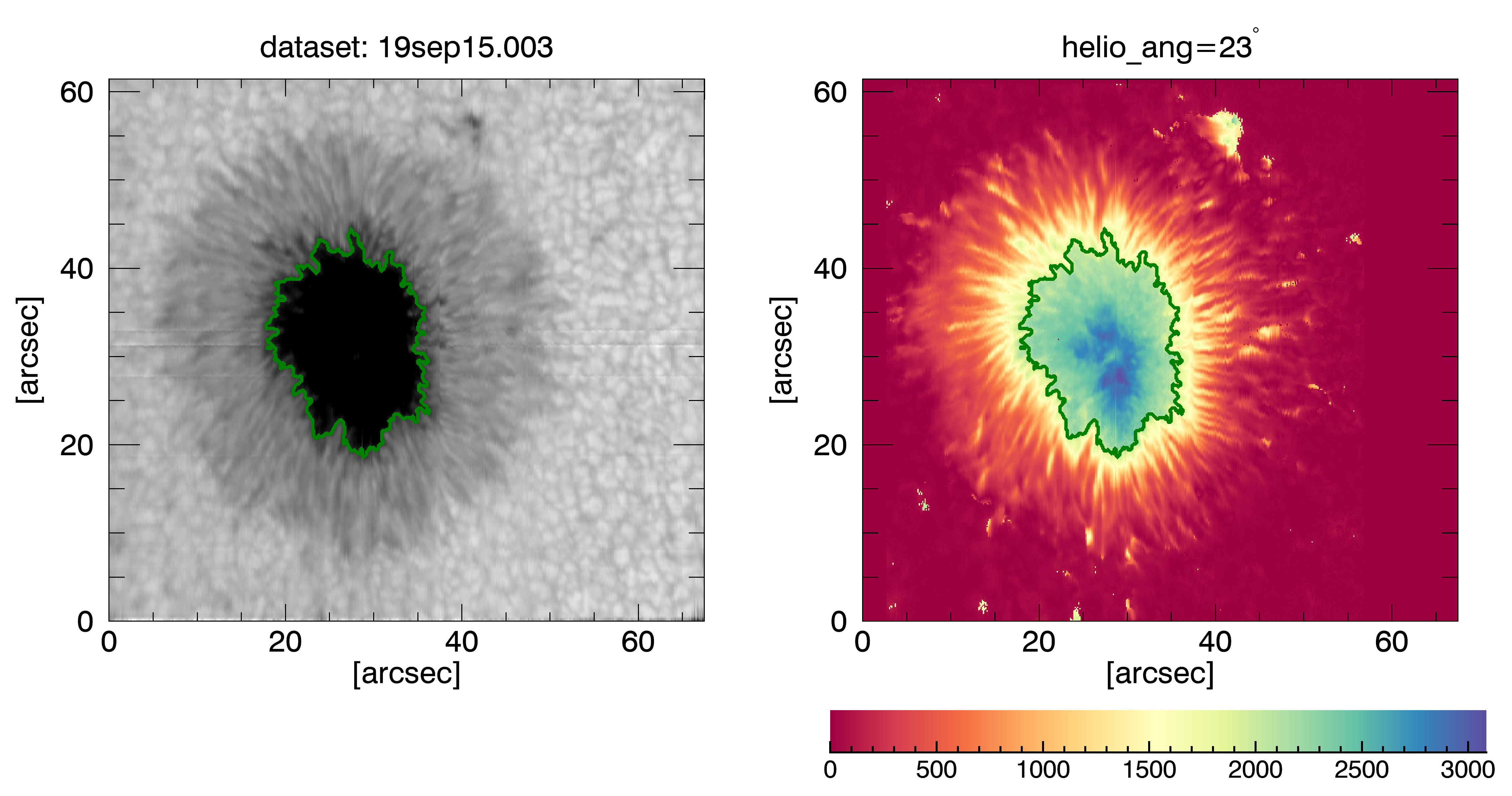
The magnetic field vector produced by the inversion was transformed from the LOS reference frame to the local reference frame (LRF) and the azimuthal ambiguity was resolved with the interactive AZAM code (Lites et al. 1995). After that, maps of $B_{\perp}$ and $B_{\parallel}$ (the component of the magnetic field that is vertical and parallel to the local surface, respectively) were calculated as $B_{\perp}=B\cdot\sin(\theta)$ and $B_{\parallel}=B\cdot\cos(\theta)$ . An example of such a map is shown in Fig. 2.

The boundary between the penumbra and umbra was first defined as a contour at a specific value in the straylight-corrected continuum intensity maps. For space-based data like Hinode, a fixed value can be used to find this contour, like done e.g. by Jurčák et al. 2018. In order to investigate whether this is possible for GRIS data, the contour level value was at first chosen manually by increasing/decreasing the value until the resulting contour was considered well outlining the umbra from a visual inspection. An example of such a contour is shown in Fig. 2.

The resulting values for each data set are shown in Table 1 and are plotted in Fig. 3. There was a difference of up to 0.09 between the values of the different data sets. However, by visual inspection we find that a change in the intensity level of more than 0.01 leads to contours that are clearly not at the umbra–penumbra boundary. This value of 0.01 also defines the error bars in Fig. 3. We therefore continued working with the manually found contours instead of using a fixed value. We ascribe the differences in contour level values mostly to different observing conditions, particularly to seeing, that alter the contrast in the intensity maps. Our straylight correction is too simple and crude to remove all the effects of seeing. In order to verify the effect of our straylight correction, we also plotted intensity level values calculated in uncorrected maps (orange data points in Fig. 3). A linear regression (slope: 0.182) showed that in the uncorrected data there was a trend towards higher $\alpha$ values being related to higher values for the intensity contour. A linear regression with the straylight corrected data (slope: -0.037) showed that while the scattering of the data remained, this trend was removed by the straylight correction.

For each data set, the median over the values of $B_{\perp}$ and $B_{\parallel}$ along the intensity contour was calculated. We denote these average quantities by $\overline{B_{\perp}}$ and $\overline{B_{\parallel}}$. Figure 5 shows these values and how they are grouped around the average value between the data sets. We identify the average value of $\overline{B_{\perp}}=$1787\text{\,}\mathrm{gauss}$$ as the critical constant below which penumbral magneto-convection can operate.
In order to compare the behavior of the averaged vertical and horizontal components of the magnetic field at the umbral boundary, i.e., $\overline{B_{\perp}}$ to $\overline{B_{\parallel}}$, Fig. 6 also shows these quantities normalized to their respective average values over the different data sets. From this visualization it becomes apparent that the $\overline{B_{\perp}}$ values are less widely spread than the $\overline{B_{\parallel}}$ values. The standard deviations of $\overline{B_{\perp}}$ and $\overline{B_{\parallel}}$ with respect to the different data sets were $\sigma_{\perp}=0.052$ and $\sigma_{\parallel}=0.126$, normalized to the average value.

Errors in our calculations come from the errors in the $B_{\perp}$ and $B_{\parallel}$ maps and from errors in finding the intensity contours. As these contours were found by choosing the corresponding level values $I_{c}$ manually and from a visual inspection, they introduce a certain subjectivity. The experience from plotting contours for many (50+) GRIS data sets showed that contours at $I_{c}\pm 0.01$ could be chosen by a different person or in a second run. We denote the corresponding contours with $C_{+}$ and $C_{-}$. In Fig. 7, these contours are plotted for two example data sets.

We calculated the difference between the average of $B_{\perp}$ over the contour $C_{+}$ to the average over contour $C_{-}$. Averaged over all data sets, the difference between these two values is $88\text{\,}\mathrm{gauss}$, which is equivalent to an uncertainty of $\pm$44\text{\,}\mathrm{gauss}$$.
Uncertainties in the $B_{\perp}$ maps have several sources. To begin with, the GRIS data (Stokes profiles) has an uncertainty. Optical properties along the beam path can also change over the years due to natural degradation and when readjusting optical elements. In addition, the seeing changes the profiles for each slit position, which translates into uncorrected straylight residuals. These errors are difficult to quantify. Furthermore, errors are introduced during our analysis. The SIR inversion code provides errors in terms of agreement between the fitted profiles and the input data, but these errors do not reflect how well the input model suits the complexity of the data. Our model assumes a magnetic field vector and a velocity that is constant in height. We chose this simplification to achieve robustness, so that the same inversion strategy can be used for all data sets. However, it does not capture the same features in the profiles that a more complex model would (e.g., three lobes in Stokes-V). Further possible error sources for the $B_{\perp}$ or $B_{\parallel}$ value of single pixels are the azimuthal disambiguation and the transformation of the magnetic field vector from the LOS to the local reference frame. As we average over contours that typically consist of around $5001000\text{\,}$ pixels, random errors are reduced for the quantities $\overline{B_{\perp}}$ and $\overline{B_{\parallel}}$.
For this study we used the difference between the contours $C_{+}$ and $C_{-}$ to derive an uncertainty of $\pm$44\text{\,}\mathrm{gauss}$$ coming from manually identifying the intensity contours. As it is difficult to calculate an exact number for the uncertainty of the $B_{\perp}$ and $B_{\parallel}$ maps including averaging over contours, we used a pragmatic approach by estimating that this uncertainty is comparable to the uncertainty in selecting the intensity contours. Conservatively rounding up, this leads to a total uncertainty of $\pm$100\text{\,}\mathrm{gauss}$$ for $\overline{B_{\perp}}$ and $\overline{B_{\parallel}}$ values. This number is to be understood as an estimate rather than a precisely calculated quantity.

Another approach to check whether a constant value of $B_{\perp}$ can serve to distinguish between umbral and penumbral magneto-convection is to compare intensity contours to contours calculated in maps of $B_{\perp}$ at this constant value. For each data set we calculated contours in maps of $B_{\perp}$ at the average value of $\overline{B_{\perp}}=$1787\text{\,}\mathrm{gauss}$$ calculated in section 3.1. In Fig. 8 these contours are compared to the manually identified intensity contours. We used the geometrical difference $\Delta P$ between these contours as a parameter to asses how well they coincide. As in Schmassmann et al. 2018, we define $\Delta P$ as the area (in pixels) that is enclosed by one of the two contours, but not the other. This value is divided by the length of the contour (in pixels) for normalization. For each data set, this value is shown in the captions of the subplots in Fig. 8. Additionally, we show a data set with a contour at $\overline{B_{\mathrm{abs}}}$ (average value of $B_{\mathrm{abs}}$ over the contours of all 11 sunspots). Like contours at average $\overline{B_{\parallel}}$ values, these contours do not outline the umbra. They are often fragmented and for large sunspots the contour lies outside the umbra–penumbra boundary, while it lies inside the umbra–penumbra boundary for smaller ones.

We analyzed the vertical component of the magnetic field $B_{\perp}$ at the boundary between umbra and penumbra. The average value over the manually found intensity contour, $\overline{B_{\perp}}$, was compared to the average of the horizontal component, $\overline{B_{\parallel}}$. The $\overline{B_{\perp}}$ values were less widely scattered between the data sets than the $\overline{B_{\parallel}}$ values (see Fig. 6), resulting in a normalized standard deviation that is 2.4 times smaller. In addition, the absolute value of the standard deviation of $\overline{B_{\perp}}$ values for the different data sets was $94\text{\,}\mathrm{gauss}$, which is in the same range as the estimated uncertainty of $100\text{\,}\mathrm{gauss}$. We therefore interpret the deviations of $\overline{B_{\perp}}$ values from the average over the data sets as being caused by our measurement uncertainty. This result is in line with the finding of $B_{\perp}$ taking a constant value at the umbra–penumbra boundary for stable sunspots (Jurčák et al. 2018).
It should be noted, however, that there are single outliers in $B_{\perp}$ values along contours of single data sets (see Fig. 4). In Fig. 8 this is seen as regions where the contour at $B_{\perp}=$1787\text{\,}\mathrm{gauss}$$ does not exactly match the intensity contours. This behavior is quantified as the geometric difference $\Delta P$. For all the data sets except 16aug16.001, this number is in the range of 2 pixels or smaller, so the deviations between the contours can be considered small. We interpret the locations where the contours do not match as regions where the umbra–penumbra boundary is not completely stable. A comparison with HMI continuum images accessed via JHelioviewer (not shown here) confirmed that the spots where the intensity contour and the contour at $B_{\perp}=$1787\text{\,}\mathrm{gauss}$$ match least closely were indeed undergoing evolution during the time of the GRIS observations. The sunspot in data set 16aug16.001, for example, expelled the pore (enclosed by the red contour but not the white one) on subsequent days. In most regions, the intensity contours and the contours at $B_{\perp}=$1787\text{\,}\mathrm{gauss}$$ match remarkably well. This is clearly not the case for contours plotted at the average value of $B_{\parallel}$ and $B_{\mathrm{abs}}$. In theses cases contours are often fragmented, and for large sunspots the contour lies outside the umbra–penumbra boundary, while it lies inside the umbra–penumbra boundary for smaller ones. An example of such a contour for one data set is shown in Fig. 8. Overall, these findings support the existence of a constant value of $B_{\perp}$ at the umbra–penumbra boundary.

In addition to providing further statistical evidence to the Jurčák criterion from ground-based observations for the first time, we obtain the critical value of $1787\pm 100\text{\,}\mathrm{gauss}$ at the umbra–penumbra boundary for GRIS data in the $1.5\text{\,}\mathrm{\SIUnitSymbolMicro m}$ (near-IR) range. Previously, this parameter had been determined only from Hinode/SP observations (Jurčák et al. 2018; Jurčák 2011) and for HMI observations (Schmassmann et al. 2018). For the Hinode/SP data (Fe I $6302\text{\,}\mathrm{\SIUnitSymbolAngstrom}$) a value of $1867^{+18}_{-16}$ $\text{\,}\mathrm{gauss}$ was derived, and for HMI (Fe I $6173\text{\,}\mathrm{\SIUnitSymbolAngstrom}$) a value of $1692\pm 15\text{\,}\mathrm{gauss}$. The question is now how to interpret the differences of $80\text{\,}\mathrm{gauss}$ (Hinode/SP) and $-95\text{\,}\mathrm{gauss}$ (HMI), respectively, from the GRIS value. It should be noted that in all three studies a certain degree of arbitrariness is introduced by either setting a fixed intensity value to define the contours in intensity (Jurčák et al. 2018; Schmassmann et al. 2018) or by defining them manually as was done in this work. This effect is not included in the respective uncertainties of the HMI and Hinode values. As shown in Sect. 3.2, differences in $\overline{B_{\perp}}$ values in the $50100\text{\,}\mathrm{gauss}$ range can be obtained by using a different intensity threshold. In this sense, all values are comparable.
In order to compare magnetic field values in general, both instrumental effects (e.g., the spectral and spatial resolution of the instrument, the seeing during the observations) and the atmospheric height ranges of the respective lines have to be considered. An overview of the parameters discussed in the following paragraphs is shown in Table 2.

References

- Balthasar (2018) Balthasar, H. 2018, Sol. Phys., 293, 120
- Benko et al. (2018) Benko, M., González Manrique, S. J., Balthasar, H., et al. 2018, A&A, 620, A191
- Berkefeld et al. (2012) Berkefeld , T., Schmidt, D., Soltau, D., von der Lühe, O., & Heidecke, F. 2012, Astronomische Nachrichten, 333, 863
- Borrero et al. (2016) Borrero, J. M., Asensio Ramos, A., Collados, M., et al. 2016, A&A, 596, A2
- Borrero & Ichimoto (2011) Borrero, J. M. & Ichimoto, K. 2011, Living Reviews in Solar Physics, 8, 4
- Collados et al. (2012) Collados, M., López, R., Páez, E., et al. 2012, Astronomische Nachrichten, 333, 872
- Collados et al. (1994) Collados, M., Martinez Pillet, V., Ruiz Cobo, B., del Toro Iniesta, J. C., & Vazquez, M. 1994, A&A, 291, 622
- Evershed (1909) Evershed, J. 1909, The Observatory, 32, 291
- Franz et al. (2016) Franz, M., Collados, M., Bethge, C., et al. 2016, A&A, 596, A4
- Garcia (2018) Garcia, M. 2018, Master Thesis at Universidad de la Laguna / Instituto de Astrofisica de Canarias / Leibniz-Institut f’́ur Sonnenphysik
- Hoeksema et al. (2014) Hoeksema, J. T., Liu, Y., Hayashi, K., et al. 2014, Sol. Phys., 289, 3483
- Jurčák (2011) Jurčák, J. 2011, A&A, 531, A118
- Jurčák et al. (2014) Jurčák, J., Bello González, N., Schlichenmaier, R., & Rezaei, R. 2014, PASJ, 66, S3
- Jurčák et al. (2015) Jurčák, J., Bello González, N., Schlichenmaier, R., & Rezaei, R. 2015, A&A, 580, L1
- Jurčák et al. (2017) Jurčák, J., Bello González, N., Schlichenmaier, R., & Rezaei, R. 2017, A&A, 597, A60
- Jurčák et al. (2018) Jurčák, J., Rezaei, R., González, N. B., Schlichenmaier, R., & Vomlel, J. 2018, A&A, 611, L4
- Lites et al. (2013) Lites, B. W., Akin, D. L., Card, G., et al. 2013, Sol. Phys., 283, 579
- Lites et al. (1995) Lites, B. W., Low, B. C., Martinez Pillet, V., et al. 1995, ApJ, 446, 877
- Ortiz et al. (2010) Ortiz, A., Bellot Rubio, L. R., & Rouppe van der Voort, L. 2010, ApJ, 713, 1282
- Rempel & Schlichenmaier (2011) Rempel, M. & Schlichenmaier, R. 2011, Living Reviews in Solar Physics, 8, 3
- Ruiz Cobo & del Toro Iniesta (1992) Ruiz Cobo, B. & del Toro Iniesta, J. 1992, ApJ, 398, 375
- Sainz Dalda (2017) Sainz Dalda, A. 2017, ApJ, 851, 111
- Schmassmann et al. (2018) Schmassmann, M., Schlichenmaier, R., & Bello González, N. 2018, A&A, 620, A104
- Schmidt et al. (2012) Schmidt, W., von der Lühe, O., Volkmer, R., et al. 2012, Astronomische Nachrichten, 333, 796
- Solanki et al. (2006) Solanki, S. K., Inhester, B., & Schüssler, M. 2006, Reports on Progress in Physics, 69, 563
- Solanki & Montavon (1993) Solanki, S. K. & Montavon, C. A. P. 1993, A&A, 275, 283
- Tiwari et al. (2013) Tiwari, S. K., van Noort, M., Lagg, A., & Solanki, S. K. 2013, A&A, 557, A25