AMC-Loss: Angular Margin Contrastive Loss for Improved Explainability in Image Classification

Hongjun Choi Anirudh Som Pavan Turaga Affiliation: Geometric Media Lab Affiliation: School of Arts, Media and Engineering, Arizona State University Affiliation: School of Electrical, Computer and Energy Engineering, Arizona State University Affiliation: hchoi71@asu.edu, asom2@asu.edu, pturaga@asu.edu

Abstract

Deep-learning architectures for classification problems involve the cross-entropy loss sometimes assisted with auxiliary loss functions like center loss, contrastive loss and triplet loss. These auxiliary loss functions facilitate better discrimination between the different classes of interest. However, recent studies hint at the fact that these loss functions do not take into account the intrinsic angular distribution exhibited by the low-level and high-level feature representations. This results in less compactness between samples from the same class and unclear boundary separations between data clusters of different classes. In this paper, we address this issue by proposing the use of geometric constraints, rooted in Riemannian geometry. Specifically, we propose Angular Margin Contrastive Loss (AMC-Loss), a new loss function to be used along with the traditional cross-entropy loss. The AMC-Loss employs the discriminative angular distance metric that is equivalent to geodesic distance on a hypersphere manifold such that it can serve a clear geometric interpretation. We demonstrate the effectiveness of AMC-Loss by providing quantitative and qualitative results. We find that although the proposed geometrically constrained loss-function improves quantitative results modestly, it has a qualitatively surprisingly beneficial effect on increasing the interpretability of deep-net decisions as seen by the visual explanations generated by techniques such as the Grad-CAM. Our code is available at https://github.com/hchoi71/AMC-Loss.

^†^†footnotetext: This work was supported in part by NSF CAREER grant number 1452163 and ARO grant number W911NF-17-1-0293.

1 Introduction

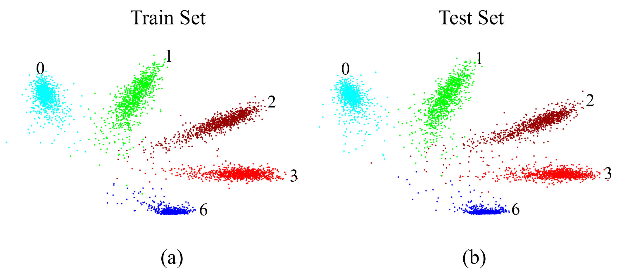
Refer to caption — Figure 1: The intrinsic ‘angular’ distribution exhibited in deep features under the cross-entropy loss in MNIST (a) train set, (b) test set where we use $10K/10K$ train/test samples for this visualization. We set the output dimension of the penultimate layer as $2$ and directly plot them in the $2$ -dimension space. We select $5$ different classes ( $0$ , $1$ , $2$ , $3$ , $6$ digits) among $10$ classes and each color denotes a class.

Deep learning methods have witnessed great success in solving classification tasks. Especially, the convolutional neural networks (CNNs) have recently drawn a lot of attention in the computer vision community due to its wide range of applications, such as object he2016deep; he2015delving, scene zhou2014object; zhou2014learning, action recognition baccouche2011sequential; ji20123d and so on. The CNN architecture is formed by a stack of convolutional layers which are a collection of filters with learnable weights and biases. Each filter creates feature maps that learn various aspects of an image to differentiate one from the other. In this regard, an essential part of training the networks is the final softmax layer to obtain the predicted probability of belonging to each class. The most common loss function used in the classification task is the cross-entropy loss which computes the cross-entropy over given probability distributions returned by the softmax layer. However, the cross-entropy loss has a few limitations since it only penalizes the classification loss and does not take into account the inter-class separability and intra-class compactness.

To address this issue, many works have gone into utilizing auxiliary loss to enhance the discriminative power of deep features along with cross-entropy loss such as center loss wen2016discriminative and contrastive loss sun2014deep_pred, where features extracted from the penultimate layer are referred to as deep features in this work. These approaches have greatly improved the clustering quality of deep features. For instance, the center loss which penalizes the Euclidean distance between deep features and their corresponding class centers is a novel technique to enforce extra intra-class distances to be minimized. Even though center loss can improve the intra-class compactness, it would not make distances between different classes not far enough apart, leading to only little changes in inter-class separability. To this end, as an alternative approach, one might want to use contrastive loss in taking into account inter-class separability at the same time. The contrastive loss can be used to learn embedding features to make similar data points close together while maintaining dissimilar ones apart from each other. However, the contrastive loss has to choose a couple of sample pairs to get the loss, so traditional contrastive loss needs careful pre-selection for data pairs (e.g, the neighboring samples/non-neighboring samples). Due to the huge scale of the training set, constructing image pairs inevitably increases the computational complexity, resulting in slow convergence during training. Furthermore, the aforementioned auxiliary loss functions have relied on the Euclidean metric in terms of approximating the semantic similarity of given samples. Meanwhile, studies verified by liu2017sphereface; wen2016discriminative hint at the fact that the deep features learned by the cross-entropy loss have an intrinsically ‘angular’ distribution as also depicted in Figure 1, thus seemingly rendering the Euclidean constraint insufficient to combine with the traditional cross-entropy loss. In summary, the weaknesses of the Euclidean contrastive loss include: a) intrinsic mismatch in geometric properties of the learnt features compared to the loss function itself, b) increases the computational complexity by constructing data pairs.

Motivated by these weaknesses, we present the following contributions: (1) First, we introduce a simple representation of images that are mapped as points on a unit-Hilbert hypersphere, which more closely matches the geometric properties of the learnt penultimate features. Also, this results in closed-form expressions to compute the geodesic distances between two points. We are able to directly deploy this geometric constraint into existing contrastive loss formulations. Indeed, our approach can deal with intrinsic angles between deep features on a hyperspherical manifold. (2) Second, designing efficient data pairs is required to compute the geodesic distance between two instances. As a result, we adopt the doubly stochastic sampled data pairs as suggested in luo2018smooth, leading to reduced overall computational cost significantly. During training, it does not require much extra time cost with $1$ - $2$ seconds per epoch.

As a preview of the results, we make the surprising finding that the proposed AMC-Loss results in more explainable interpretations of deep-classification networks, when input activation maps are visualized by the technique of Grad-CAM selvaraju2017grad. Generally, the blue regions indicate small or inhibitory weights while the red regions represent large or excitatory weights. Interpreting what parts of the input are most important for the final decision is crucial to make deep-nets more explainable and interpretable. For instance, as seen in Figure 2, we generated the activation maps from the model trained by three different loss functions, the cross-entropy loss, the Euclidean contrastive loss with cross-entropy loss (refer to this loss as + Eucd in the rest of the paper) and AMC-Loss with cross-entropy loss (denote this by + AMC-Loss) respectively. In the airplane image, the Euclidean variants seem to be reacting to the body parts of the airplane, but also to the sky. The proposed AMC-Loss results in a more tightly bounded activation map. Based on additional visualization shown later in section 4, it appears that the cross-entropy loss pays attention to important parts of objects, but also pays attention to a lot of background information. The Euclidean contrastive loss, when combined with the basic cross-entropy, leads to fuzzy and generally un-interpretable activation maps. Whereas, the addition of the AMC-Loss results in more compact maps that are also interpretable as distinct object parts, while also reducing the effect of the background.

The rest of the paper is outlined as follows: Section 2 provides a background study. In Section 3, we describe the proposed framework in detail and in Section 4 we provide both qualitative and quantitative results. Section 5 concludes the paper.

2 Background

The cross-entropy loss together with softmax activation is one of the most widely used loss functions in image classification hinton2012improving; he2016deep; he2015delving. Following this, many joint supervision loss functions with cross-entropy loss have been proposed to generate more discriminative features wen2016discriminative; sun2014deep_pred; luo2018smooth. In this section, we focus on revisiting these typical loss functions including related spherical-type loss.

Cross-entropy Loss

The cross-entropy loss function is defined as: $L_{C}=-\frac{1}{N}\sum_{i=1}^{N}\log\frac{e^{W^{T}_{y_{i}}x_{i}+b_{y_{i}}}}{\sum_{j=1}^{n}e^{W^{T}_{j}x_{i}+b_{j}}},$ where, $x_{i}\in\mathbb{R}^{d}$ denotes the deep features of the $i$ -th image, belonging to the $y_{i}$ -th class. $W_{j}\in\mathbb{R}^{d}$ represents the $j$ -th column of the weights $W\in\mathbb{R}^{d\times n}$ and $b_{j}\in\mathbb{R}^{n}$ is the bias term. The batch size and the class number are $N$ and $n$ , respectively. Although the cross-entropy loss is widely used, it does not explicitly optimize the embedding feature to maximize inter-class distance, which results in a performance gap under large intra-class variations.

Contrastive loss

To address this issue, many related works have attempted to train the network with an auxiliary loss and a cross-entropy loss simultaneously during training. For instance, Yi et al. sun2014deep proposed the contrastive loss for face recognition to enforce inter-class separability while preserving intra-class compactness. In specific, one needs to carefully select data pairs to be grouped into neighboring and non-neighboring samples beforehand. That is, if samples belong to the neighbors, the matrix $S_{ij}$ which measures the similarity between samples sets to $1$ , otherwise $S_{ij}$ sets to $0$ , meaning samples of different classes. We then denote the contrastive loss as:

L_{E}=\begin{cases}\left\|x_{i}-x_{j}\right\|^{2}&\text{if }S_{ij}=1\\ \max(0,m_{e}-\left\|x_{i}-x_{j}\right\|)^{2},&\text{if }S_{ij}=0\end{cases}

(1)

where $m_{e}>0$ is a pre-defined Euclidean margin and $\left\|\cdot\right\|$ is the Euclidean distance between deep features $x_{i}$ and $x_{j}$ . Consequently, the neighboring samples are encouraged to minimize their distances while the non-neighboring samples are pushed apart from each other with a minimum distance of $m_{e}$ . The value $m_{e}$ is the margin of separation between neighbors and non-neighbors and can be decided empirically. When $m_{e}$ is large, it pushes dissimilar and similar samples further apart thus acting as a margin.

Spherical-type Loss

The existing contrastive loss adopts the Euclidean metric on deep features. However, as mentioned in the previous section, the Euclidean-based loss functions are incompatible with the cross-entropy loss due to intrinsic angular distributions visible in deeply learned features as presented in Figure 1. Weiyang et al. liu2017sphereface proposed SphereFace to address this issue by introducing angles between deep features and their corresponding weights in a multiplicative way for a face recognition task. For example, for binary class case, the decision boundary for class $1$ and class $2$ become $\left\|\mathbf{x}\right\|(\cos(m\theta_{1})-cos(\theta_{2}))$ and $\left\|\mathbf{x}\right\|(\cos(\theta_{1})-cos(m\theta_{2}))$ where $m$ quantitatively controls the angular margin and $\theta$ is the angle between weight $\mathbf{W}_{i}$ and feature vector $\mathbf{x}$ . Other avenues proposed alternatives to softmax by exploring a spherical family of functions: the spherical softmax and Taylor softmax de2015exploration. In spherical softmax, one replaces the exponential function by a quadratic function and the Taylor softmax replaces the exponential function by the second-order Taylor expansion. These alternative formulations allow us to compute exact gradients without computing all the logits, leading to reducing the cost of computing gradients. Although they showed that these functions do not outperform when the length of an output vector is large e.g, in language modeling tasks with large vocabulary size, they surpassed the traditional softmax on MNIST and CIFAR10 dataset. Our work is complementary to these and can be combined with them in that AMC-Loss intuitively respects the angular distributions empirically observed in deep features.

3 Proposed Method

In this section, we elaborate on our approach. A brief overview of the proposed framework for image classification tasks is shown in Figure 3. The CNNs take the input that is passed through a stack of convolutional (Conv. $1,2,3$ ) layers, where the filters were used with a small receptive field: $3\times 3$ . At the last configuration, it utilizes $1\times 1$ convolution filters, which can be seen as a linear transformation of the input channels. The max pooling is performed over a $2\times 2$ pixel window. The final convolutional layer is then fed to a global average pooling layer, which yields a vector, called a deep feature in this paper. Based on the proposed method, this deep feature is represented as a point on the hypersphere by restricting unit-norm features $z_{i}=x_{i}/\left\|x_{i}\right\|$ , and apply them to the AMC-Loss. The final fully connected layer has a softmax activation function to produce the predicted probability of each class. Finally, the cross-entropy loss function can be used along with AMC-Loss. That is, during training, our approach estimates a particular embedding position for an image by the hypersphere representations and updates the parameters through the network such that it keeps similar points together and dissimilar ones apart by penalizing the geodesic distance between given two points, $d(z_{i},z_{j})=\cos^{-1}\langle\,z_{i},z_{j}\rangle$ .

3.1 AMC-Loss

Intuitively, AMC-Loss minimizes the geodesic distance for points of the same class while encouraging points of different classes to have a more distinct separation with a minimum angular margin $m_{g}$ . To this end, we propose the AMC-Loss while preserving the existing contrastive loss formulation, as formulated in (2).

\displaystyle L_{A}=\begin{cases}(\cos^{-1}\langle\,z_{i},z_{j}\rangle)^{2}&\text{if }S_{ij}=1\\ \max(0,m_{g}-\cos^{-1}\langle\,z_{i},z_{j}\rangle)^{2}&\text{if }S_{ij}=0\end{cases}

(2)

where, instead of the Euclidean margin $m_{e}$ , $m_{g}>0$ becomes an angular margin. In (2), $S_{ij}=0$ is assigned to non-neighboring pairs whereas $S_{ij}=1$ is allotted to neighboring pairs. Ideally, all possible training sample combinations can be considered in the matrix $S_{ij}$ . However, due to the large size of training pairs, instead of updating parameters with respect to the entire training set, we perform the update based on a mini-batch. The CNN model is iteratively optimized using gradient descent by joint-supervision with the cross-entropy loss and the AMC-Loss. Even though we perform updates at the mini-batch level, it still involves the computational burden to compute the geodesic distance for all combinations of samples in a batch – thereby resulting in slow-convergence during training.

Specifically, constructing the matrix $S_{ij}$ involving all data pairs $(x_{i},x_{j})\in B$ where mini-batch $B$ is of size $n$ , requires $\mathcal{O}(n^{2})$ computations in total. Also, computing geodesic distance between two points related to $S_{ij}$ is $\mathcal{O}(p)$ where $p$ denotes $p$ -dimensional vector, resulting in the overall computational cost of $\mathcal{O}(n^{2}p)$ , which is slow for large $n$ . To address this issue, following luo2018smooth, we adopt the doubly stochastic sampled data pairs in computing the geodesic. In each iteration, we sample a mini-batch $B$ into two groups, $B_{1}$ and $B_{2}$ groups, where each group has $n/2$ samples. Then we are able to directly compare two groups and compute corresponding geodesic distance element-wise. Finally, the overall cost can be reduced down to $\mathcal{O}(\frac{np}{2})$ . Additionally, without the need for pre-selection for data pairs beforehand, we can build the matrix $S_{ij}$ based on the predicted labels from the output of networks $\tilde{f}$ as follows:

\displaystyle S_{ij}=\begin{cases}1&\text{if }\tilde{y}_{i}=\tilde{y}_{j}\\ 0&\text{if }\tilde{y}_{i}\neq\tilde{y}_{j}.\end{cases}

(3)

The predicted label corresponding to $i$ -th input image is given by $\tilde{y}_{i}=\text{argmax}_{k}[\tilde{f}_{i}]_{k}$ , where $\text{argmax}_{k}[\cdot]_{k}$ directly indicates the class label having the maximum probability among classes. We present the pseudo-code in algorithm 1.

Algorithm 1 Mini-batch training of AMC-Loss

Input: $x_{i}$ = training inputs, $y_{i}$ corresponding input labels
Require: $z_{i}$ = normalized deep feature of $x_{i}$
Require: $w(t)$ = weight function
Require: $f_{\theta}(x)$ = CNNs with parameter $\theta$

1: for

t

[1,\text{num\_epochs}]

2: for each minibatch

B

\tilde{f}_{i}

\leftarrow

f(x_{i}\in B)

4: for

(x_{i},x_{j})

in a minibatch pairs from

B

5: compute

S_{ij}

based on Eq. 3.

6: loss

\leftarrow

L_{C}

7: +

w(t)[\lambda\frac{1}{|B|}\sum_{i,j\in B}L_{A}(z_{i},z_{j},S_{ij})

8: update

\theta

using optimizers (Adam)

9: return

\theta

Clearly, the CNNs supervised by AMC-Loss are trainable and can be optimized by standard SGD. A scalar $\lambda$ denotes the balancing parameter between the cross-entropy loss and $L_{A}$ . We additionally conduct experiments to illustrate how the balancing parameter $\lambda$ and angular margin $m_{g}$ influence performance in section 4.3. As the weight function $w(t)$ , we use the Gaussian ramp-up and ramp-down curve to put weights on $L_{A}$ during training. We describe this weight function in more detail next.

3.2 Training Details

We implemented our code in Python $3.7$ with Tensorflow $1.12.0$ . All models including baseline have been trained for $300$ epochs using Adam optimizer with mini-batch of size $n=128$ and maximum learning rate $0.003$ . We use the default Adam momentum parameters $\beta_{1}=0.9$ and $\beta_{2}=0.999$ . Following laine2016temporal, we ramp up the weight parameter $w(t)$ and learning rate during the first $80$ epoch with weight $w(t)=\exp[-5(1-\frac{t}{80})^{2}]$ and ramp down the learning rate and Adam $\beta_{1}$ to $0.5$ during the last 50 epochs. The ramp-down function is $\exp[-12.5(1-\frac{300-t}{50})^{2}]$ . The balancing coefficient of $\lambda$ is set to $0.1$ in all experiments. To compare with the Euclidean contrastive loss, we keep the same architecture and other hyper-parameters settings with $\lambda=0.1$ and $m_{e}=1.0$ . The Euclidean margin $m_{e}=1.0$ and angular margin $m_{g}=0.5$ were chosen from different variations, leading to the best performance.

4 Experiments

In this section, we show the effectiveness of the AMC-Loss by visualizing deep features in Section 4.1 and presenting the classification accuracy on several public datasets in Section 4.2 with a supportive visualization result. Then we investigate the sensitiveness of the balancing parameter $\lambda$ and the angular margin $m_{g}$ in Section 4.3.

4.1 Improved Clustering

As our proposed framework encourages the deep features to be discriminative on the hyperspherical manifold, we trained the model with the proposed loss function by restricting the feature dimension to three for more intuitive visualization on a sphere. The learnt features are shown in Figure 4. We measure the clustering performance based on the following metrics rosenberg2007v:

Homogeneity: A clustering result satisfies homogeneity if all of its clusters contain only data points that are members of a single class.

Completeness: A clustering result satisfies completeness if all the data points that are members of a given class are elements of the same cluster.

Further, we visualize the deep features learned by AMC-Loss and compare them with learnt features by baseline models on SVHN test data by projecting them to $2$ -dimensions using tSNE maaten2008visualizing in Figure 5. As we can see in this plot, the features learned by + AMC-Loss are more separable for inter-class samples and more compact for intra-class samples as also seen in homogeneity and completeness.

4.2 Image Classification

Besides feature representations, we tabulate classification performance on the benchmark dataset in Table 1. The reported results are averaged over $5$ runs. In order to check the significance of the proposed method, we calculate the p-value with respect to only + Eucd so that we directly compare the Euclidean constraint with the proposed geometric constraint. The p-value is the area of the two-sided $t$ -distribution that falls outside $\pm t$ . Although + AMC-Loss does not yield as good results as the + Eucd on MNIST dataset, it outperforms + Eucd on other datasets with p-value of less than $0.05$ .

Model	MNIST		CIFAR10
Model	Mean $\pm$ SD	p-Value	Mean $\pm$ SD	p-Value
Cross-entropy	99.63 $\pm$ 0.01	-	82.35 $\pm$ 0.17	-
+ Eucd	99.65 $\pm$ 0.01	-	82.60 $\pm$ 0.21	-
+ AMC-Loss	99.66 $\pm$ 0.01	0.1525	82.97 $\pm$ 0.20	0.0214

Model	SVHN		CIFAR100
Model	Mean $\pm$ SD	p-Value	Mean $\pm$ SD	p-Value
Cross-entropy	94.03 $\pm$ 0.11	-	65.16 $\pm$ 0.12	-
+ Eucd	95.29 $\pm$ 0.06	-	65.57 $\pm$ 0.20	-
+ AMC-Loss	95.52 $\pm$ 0.05	0.0002	66.19 $\pm$ 0.22	0.0016

Table 1: Classification results on benchmark datasets, averaged over 5 runs. p-values are calculated with respect to the + Eucd baseline model.

MNIST. It consists of the $60,000$ gray-scale training images and $10,000$ test images from handwritten digits $0$ to $9$ .

CIFAR10. The CIFAR10 dataset consists of $32\times 32$ natural RGB images from $10$ classes such as airplanes, cats, cars and horses and so on. We have $50,000$ training examples and $10,000$ test examples.

CIFAR100. The CIFAR100 dataset consists of $32\times 32$ natural RGB images, but they have $20$ super-class (coarse label) and $100$ classes (fine label). Note, we evaluate the performance with $20$ super-class.

SVHN. Each example in SVHN is $32\times 32$ color house-number images and we use the official $73,257$ training images and $26,032$ test images.

We provide the activation maps of test images per class in Figure 6. In this figure, the AMC-Loss shows qualitatively better performance, in the sense that foreground objects become more distinct and salient with high weights while focusing less on the background. On the other hand, the + Eucd loss, including the cross-entropy loss, appears more spread out and less ‘on target’. By emphasizing important regions, the AMC-Loss may bring out stronger explainable performance.

4.3 Robustness to Parameter Tuning

We evaluate our model to see sensitivity to the balancing parameter $\lambda$ and the angular margin $m_{g}$ on the CIFAR10 dataset. The hyper-parameter $\lambda$ controls the balance between the cross-entropy loss and AMC-Loss and $m_{g}$ determines the minimum angular distance of how far points of non-neighbors are pushed apart. Both of them are essential to our model. We first fix $m_{g}$ to $0.5$ and vary $\lambda$ from $1$ to $0.001$ to learn different models. Likewise, we evaluate the performance by varying angular margin from $0.5$ to $1.5$ with fixed $\lambda=0.1$ . The trend accuracy of these models is shown in Figure 7 along with the p-value.

5 Conclusion

In this work, we have studied a simple analytic geometric constraint imposed on the penultimate feature layer, motivated by empirical observations of the shape of feature distributions. The proposed AMC-loss is a more natural way to introduce the contrastive term in combination with the traditional cross-entropy loss function. By representing image features as points on hypersphere manifold, we have shown that deep features learned by the angular metric can enhance discriminative power modestly. More importantly, we find that the use of the AMC-loss results in models that are seemingly more explainable. This is a rather unexpected finding. As seen in our experiments, the proposed method can enable deep features to be more distinct by improving localization of important regions. Our work is complementary to similar efforts that impose spherical-type losses; the AMC-Loss extends these ideas into contrastive losses, while showing that the resultant deep-net is more explainable.

Appendix A Network architectures

Input: $32\times 32\times 3$ image for CIFAR10, SVHN, CIFAR100
Add Gaussian noise $\sigma$ = $0.15$
$3\times 3$ conv. 128 lReLU ( $\alpha=0.1$ ) same padding
$3\times 3$ conv. 128 lReLU ( $\alpha=0.1$ ) same padding
$3\times 3$ conv. 128 lReLU ( $\alpha=0.1$ ) same padding
$2\times 2$ max-pool, dropout $0.5$
$3\times 3$ conv. 256 lReLU ( $\alpha=0.1$ ) same padding
$3\times 3$ conv. 256 lReLU ( $\alpha=0.1$ ) same padding
$3\times 3$ conv. 256 lReLU ( $\alpha=0.1$ ) same padding
$2\times 2$ max-pool, dropout $0.5$
$3\times 3$ conv. 512 lReLU ( $\alpha=0.1$ ) valid padding
$1\times 1$ conv. 256 lReLU ( $\alpha=0.1$ )
$1\times 1$ conv. 128 lReLU ( $\alpha=0.1$ )
Global average pool $6\times 6$ $\rightarrow$ $1\times 1$
Fully connected $128$ $\rightarrow$ $10$ softmax
Input: $28\times 28\times 1$ image for Figure 1 and Figure 4
Add Gaussian noise $\sigma$ = $0.15$
$3\times 3$ conv. 64 lReLU ( $\alpha=0.1$ ) same padding
$2\times 2$ max-pool, dropout $0.5$
$3\times 3$ conv. 64 lReLU ( $\alpha=0.1$ ) same padding
$2\times 2$ max-pool, dropout $0.5$
$3\times 3$ conv. 128 lReLU ( $\alpha=0.1$ ) valid padding
$1\times 1$ conv. 64 lReLU ( $\alpha=0.1$ ) same padding
Global average pool $5\times 5$ $\rightarrow$ $1\times 1$
Fully connected 3 $\rightarrow$ $10$ softmax

Table 2: The network architectures used in all experiments. The output of the global average pooling layer is

128

for all experiments(exceptions are Figure 1 with

2

-dimension and Figure 4 with

3

-dimension).

As suggested in laine2016temporal; luo2018smooth, we use the same CNN architectures for our experiments, but we use standard batch normalization. The architecture in the top panel of Table 2 is used to produce results for Figures 5, 2, and 7, and Table 1. The bottom architecture is used for Figure 1 and 4. For the angular distribution in Figure 1 and the spherical representation in Figure 4, we trained the model for $150$ epochs using Adam Optimizer with batch size of $128$ and maximum learning rate $0.003$ . We apply ramp up during the first $40$ epochs and ramp down for the last $30$ epochs.

References

(1) Moez Baccouche, Franck Mamalet, Christian Wolf, Christophe Garcia, and Atilla Baskurt. Sequential deep learning for human action recognition. In International workshop on human behavior understanding, pages 29–39. Springer, 2011.
(2) Alexandre de Brébisson and Pascal Vincent. An exploration of softmax alternatives belonging to the spherical loss family. arXiv preprint arXiv:1511.05042, 2015.
(3) Kaiming He, Xiangyu Zhang, Shaoqing Ren, and Jian Sun. Delving deep into rectifiers: Surpassing human-level performance on imagenet classification. In Proceedings of the IEEE international conference on computer vision, pages 1026–1034, 2015.
(4) Kaiming He, Xiangyu Zhang, Shaoqing Ren, and Jian Sun. Deep residual learning for image recognition. In Proceedings of the IEEE conference on computer vision and pattern recognition, pages 770–778, 2016.
(5) Geoffrey E Hinton, Nitish Srivastava, Alex Krizhevsky, Ilya Sutskever, and Ruslan R Salakhutdinov. Improving neural networks by preventing co-adaptation of feature detectors. arXiv preprint arXiv:1207.0580, 2012.
(6) Shuiwang Ji, Wei Xu, Ming Yang, and Kai Yu. 3d convolutional neural networks for human action recognition. IEEE transactions on pattern analysis and machine intelligence, 35(1):221–231, 2012.
(7) Samuli Laine and Timo Aila. Temporal ensembling for semi-supervised learning. arXiv preprint arXiv:1610.02242, 2016.
(8) Weiyang Liu, Yandong Wen, Zhiding Yu, Ming Li, Bhiksha Raj, and Le Song. Sphereface: Deep hypersphere embedding for face recognition. In Proceedings of the IEEE conference on computer vision and pattern recognition, pages 212–220, 2017.
(9) Yucen Luo, Jun Zhu, Mengxi Li, Yong Ren, and Bo Zhang. Smooth neighbors on teacher graphs for semi-supervised learning. In Proceedings of the IEEE conference on computer vision and pattern recognition, pages 8896–8905, 2018.
(10) Laurens van der Maaten and Geoffrey Hinton. Visualizing data using t-sne. Journal of machine learning research, 9(Nov):2579–2605, 2008.
(11) Andrew Rosenberg and Julia Hirschberg. V-measure: A conditional entropy-based external cluster evaluation measure. In Proceedings of the 2007 joint conference on empirical methods in natural language processing and computational natural language learning (EMNLP-CoNLL), pages 410–420, 2007.
(12) Ramprasaath R Selvaraju, Michael Cogswell, Abhishek Das, Ramakrishna Vedantam, Devi Parikh, and Dhruv Batra. Grad-cam: Visual explanations from deep networks via gradient-based localization. In Proceedings of the IEEE international conference on computer vision, pages 618–626, 2017.
(13) Yi Sun, Yuheng Chen, Xiaogang Wang, and Xiaoou Tang. Deep learning face representation by joint identification-verification. In Advances in neural information processing systems, pages 1988–1996, 2014.
(14) Yi Sun, Xiaogang Wang, and Xiaoou Tang. Deep learning face representation from predicting 10,000 classes. In Proceedings of the IEEE conference on computer vision and pattern recognition, pages 1891–1898, 2014.
(15) Yandong Wen, Kaipeng Zhang, Zhifeng Li, and Yu Qiao. A discriminative feature learning approach for deep face recognition. In European conference on computer vision, pages 499–515. Springer, 2016.
(16) Bolei Zhou, Aditya Khosla, Agata Lapedriza, Aude Oliva, and Antonio Torralba. Object detectors emerge in deep scene cnns. arXiv preprint arXiv:1412.6856, 2014.
(17) Bolei Zhou, Agata Lapedriza, Jianxiong Xiao, Antonio Torralba, and Aude Oliva. Learning deep features for scene recognition using places database. In Advances in neural information processing systems, pages 487–495, 2014.