Revealing Cluster Structures Based on
Mixed Sampling Frequenciesii
i
Opinions expressed herein are those of the authors alone and do not necessarily reflect the views of the Federal Reserve System.
We thank Gianni Amisano, Eric Ghysels, Michael Owyang and the participants of Midwest Econometrics Group 2018 Meeting, the joint meeting of 11th International Conference of the ERCIM WG on Computational and Methodological Statistics and 12th International Conference on Computational and Financial Econometrics, and the Federal Reserve System Econometrics conference in 2020. Rho and Liu are partially supported by NSF-CPS grant #1739422.
A primitive version of this paper had been circulated under the title “Panel Nonparametric MIDAS Model: A Clustering Approach” by the first two authors.
Yeonwoo Rho1, Yun Liu2, and Hie Joo Ahn3 iiii ii Emails: Y. Rho (yrho@mtu.edu), Y. Liu (AnnaLiu@quickenloans.com), and H. Ahn (HieJoo.Ahn@frb.gov)
1Michigan Technological University
2Quicken Loans
3Federal Reserve Board
August 11, 2026
Abstract
This paper proposes a new linearized mixed data sampling (MIDAS) model and develops a framework to infer clusters in a panel regression with mixed frequency data. The linearized MIDAS estimation method is more flexible and substantially simpler to implement than competing approaches. We show that the proposed clustering algorithm successfully recovers true membership in the cross-section, both in theory and in simulations, without requiring prior knowledge of the number of clusters. This methodology is applied to a mixed-frequency Okun’s law model for state-level data in the U.S. and uncovers four meaningful clusters based on the dynamic features of state-level labor markets.
key words: Clustering; forecasting; mixed data sampling regression model; panel data; penalized regression.
1 Introduction
Following technological advances, the diffusion of social media, and the efforts of statistical agencies and private companies, new data sources have recently become available for empirical research in economics. In many cases, these data are characterized by large time series and cross sectional dimensions, with detailed information on economic agents often at a level of disaggregation more granular than that of traditional data sources. Due to the increasing availability of richer cross-section data, it has become particularly important to efficiently summarize and identify the most important features of subjects in the cross-section. With the increased capacity in handling higher sampling frequency data, the mixed data sampling (MIDAS) models (e.g., Ghysels et al. 2007) are now widely used in practical applications in forecasting variables that inherently have a low sampling frequency. One of the purposes of MIDAS models is to understand how high-frequency variables are related to the low-frequency variables of interest, which is essentially captured by the shape of MIDAS weight function. With the aim of properly accounting for unit heterogeneity, this paper proposes a new empirical method to identify distinct groups in a panel data based on their MIDAS weights.
Previous studies on MIDAS models with panel data (e.g. Andreou et al. 2010) arbitrarily divided observations into different groups. This approach crucially depends on prior knowledge and homogeneity within each group is not necessarily guaranteed. To avoid such issues, we propose to construct an entirely data-driven clustering algorithm by adapting Ma and Huang 2017’s clustering idea to a panel setting. This clustering is based on how close coefficient estimations are between subjects in the panel. Closer estimates are penalized, resulting in unanimous coefficient estimates within the same cluster. An important feature of this clustering idea is that the clustering procedure is entirely data-driven, including the number of clusters.
The proposed clustering algorithm can be combined with, in principle, any MIDAS models.iiiiii iii This is because the proposed clustering algorithm can be applied to a general panel data setting. In this paper, we focus on its applications to mixed frequency settings for brevity. In practice, however, the accompanying MIDAS estimation procedure needs to be computationally efficient. This is because the penalized regression idea of Ma and Huang 2017 requires a complicated optimization process as well as grid searches of a few tuning parameters. Unfortunately, existing MIDAS models are either too complicated or too time-consuming to be used in combination with the clustering methods with penalized regression. In parametric MIDAS models, arbitrary parametric functions (e.g., exponential Almon lag function, beta function) are used to model the coefficients on high-frequency variables. As these parametric functions are highly nonlinear in general, complicated numerical optimization is required for estimation. As this estimation is numerically costly and challenging, practitioners often give MIDAS models a wide berth. The recently proposed nonparametric MIDAS model by Breitung and Roling 2015 does not require any arbitrary choice of parametric functional forms in specifying the distributed lags structure of the coefficients on high frequency variables. However, the tuning parameters of Breitung and Roling 2015’s methodology require demanding numerical search, which adds heavy computational burden to the proposed clustering algorithm.
This paper fills this gap in the literature by devising a novel linearized MIDAS model based on the Fourier flexible form and polynomials. The Fourier flexible form and polynomials allow the trajectory of coefficients on high-frequency variables to be flexibly determined by the data. Our model requires just ordinary least squares (OLS), which eschews estimation difficulty. Unlike Breitung and Roling 2015’s methodology, the tuning parameters involved with our method do not require heavy computations. In addition, an arbitrary choice of these tuning parameters work reasonably well, a powerful feature when combining MIDAS models with the proposed clustering method.
Simulations conducted in this paper show many desirable features of our method. First, the proposed linearized MIDAS model tends to provide better one-step-ahead forecasts than Breitung and Roling 2015.iviv iv Since Breitung and Roling 2015 reported better estimation and forecasting results of their method compared to parametric MIDAS models, we can infer that our method would also have a similar advantage to the parametric MIDAS. Second, for our MIDAS method, an arbitrary choice of tuning parameters works reasonably well, thought it can be further improved by a data-driven choice. Third, our MIDAS clustering method is faster in computation and yields more precise parameter estimation and better forecasting properties than other clustering approaches in the data environment of mixed-sampling frequencies.
As a relevant empirical application, we use our method to explore heterogeneity in labor market dynamics across states in the U.S. using a mixed-frequency panel Okun’s law model. Okun’s law is an empirical relationship that relates changes in unemployment rate to GDP growth. Usually an Okun’s law model is specified at quarterly frequency, as GDP growth is available only quarterly. In our application, we include weekly initial claims of unemployment insurance (UI) benefits as the high-frequency indicator, which is known as the most timely indicator of job losses. By doing so, the model can better characterize the sudden rise in unemployment rate at the onset of a recession, picking up sudden bursts in layoffs. An additionally desirable feature of the mixed-frequency Okun’s law model is that it can be used to nowcast the unemployment rate at the state level on a weekly basis.
The algorithm identifies four clusters among states based on the responsiveness of unemployment rate to GDP growth and on the pattern of coefficients on weekly initial claims within the quarter. The coefficients on GDP growth and initial claims most likely reflect the structural aspects of state-level labor markets (e.g. the industry composition) and the local labor-market practices of hirings and layoffs. Hence, the clusters identified by the model most likely capture relevant heterogeneity in the functioning of labor markets in different states.
We relate the identified clusters to observable state–level attributes such as the small-firms employment share, industry composition, the relevance of oil production, and the share of long-term unemployment out of total unemployment. Each cluster exhibits multi-dimensional attributes, suggesting that the differences in labor-market dynamics across states cannot be determined or accurately summarized by one or two observable factors. Another way to say this is that the clustering algorithm is able to capture a state’s unobserved attributes which are not fully reflected in the data but are nevertheless crucial for unemployment dynamics. In this regard, our proposed methodology can reveal similarities and differences across states in the functioning of their labor markets purely based on the data, and can provide a new understanding of regional heterogeneity in labor market dynamics.
The rest of this paper is organized as follows. Section 2 introduces the proposed linearized MIDAS approach using the Fourier flexible form and polynomials. Subsection 2.1 introduces the linearized MIDAS estimation in a non-panel setting. Subsection 2.2 demonstrates our linearized MIDAS method’s estimation and forecasting accuracy in finite samples. Section 3 presents the clustering algorithm. The proposed clustering approach accompanied with our MIDAS method delivers accurate estimates, as proven in theory and shown in the finite sample simulations. Section 4.1 provides an empirical application of the method. Details on algorithms used in simulations and technical proofs are relegated to Sections A and B, respectively, in the supplementary material.
The following notation will be used throughout the paper. The -norm of a vector is . For an matrix with its th element being , indicates the -norm induced by the corresponding vector norm. That is, . In particular, and . For a symmetric and positive definite matrix , let and indicate the smallest and largest eigenvalues of , respectively. It is worth noting that . is a identity matrix and denotes the Kronecker product. For any real number , denotes the largest integer that is smaller than or equal to . The symbol denotes the indicator function.
2 Linearized MIDAS
In this section, we introduce our linearized MIDAS approach using the Fourier flexible form [Gallant 1981]. We first introduce the framework, then confirm that the proposed linearized MIDAS model is a good approximation of popular parametric MIDAS models in finite samples.
2.1 Linearized MIDAS with the Fourier flexible form and polynomials
Consider the following MIDAS model with the forecast lead :
| (1) |
for . Here, is the -vector of low-frequency covariates at time , and is the corresponding coefficient vector. The vector is the high-frequency variable at and are the coefficients that aggregate to the low-frequency. In a parametric MIDAS model, the coefficients can be written as a multiple of , where weights are assumed to be generated by, for example, an exponential Almon lag function
and and are parameters that need to be estimated from data. However, the form of is somewhat limited, and it requires nonlinear estimation. In this paper, we propose to model using the Fourier flexible form and polynomials. The MIDAS coefficients are assumed to be generated by
| (2) |
for some positive integers and . The Fourier flexible form has been frequently used in macroeconomics and finance since Gallant 1981. It has been demonstrated that the Fourier flexible form is capable of approximating most forms of nonlinear time trends to any degree of accuracy if a sufficient number of parameters is used, and that a small is often enough to reasonably approximate smooth functions with finite numbers of breaks [Becker et al. 2004, Becker et al. 2006, Enders and Lee 2012, Rodrigues and Robert Taylor 2012, Güriş 2017, Perron et al. 2017]. In addition to the Fourier flexible form, we also consider a few polynomial trends to cover wider range of nonlinear functions, following suggestions in Perron et al. 2017.vv v Our approach assumes that the underlying nonlinear MIDAS weight function can be approximated by (2) with fixed and . If as , it is well-known that any bounded function can be precisely approximated by (2); in this case, the proposed MIDAS model can be considered nonparametric. However, as seen in our simulations, (2) works reasonably well with an arbitrary choice of relatively small and . In this paper, we choose to make our argument with fixed and , and call our method “linearlized” to emphasize its computational advantage and its ability to concisely represent a wide range of nonlinear MIDAS weight functions.
The MIDAS model (1) with the Fourier flexible form (2) can be expressed as
where , , , , , , and
| (3) |
Here, the matrix can be understood as a Fourier transform operator. This Fourier transformation summarizes the information in an -dimensional vector into a -dimensional vector where , and are transformed high-frequency data for and , and are defined as , , and vivi vi Note that can effectively summarize the information in , because relatively small and are enough to capture main characteristics of a nonlinear trend function. For instance, Enders and Lee 2012 reported that even a single frequency allows for multiple smooth breaks..
Unlike parametric MIDAS models, this model is linear. Noting that , the ordinary least squares (OLS) estimator of can be written as
| (4) |
where , and is an identity matrix. Under some regularity conditions, can be estimated consistently by the OLS estimator .
2.2 Simulation: linearized MIDAS
This subsection consists of two parts. The first part compares our proposed linearized MIDAS estimation with an existing nonparametric MIDAS [Breitung and Roling 2015]. Breitung and Roling 2015 imposes a smoothness condition on , which involves a tuning parameter. In our simulations, their tuning parameter is chosen by a modified Akaike information criterion (AIC) as proposed in Breitung and Roling 2015. See Section A.1 in the supplementary material for more details. Our method is based on a generic choice of and with and . The second part of this subsection investigates if data-driven choices of and can improve the quality of our linearized MIDAS estimation.
The simulation setting considered in the first part is similar to that of Breitung and Roling 2015. For ,
| (5) |
where , , , , , , and the frequency ratio . For the AR(1) high-frequency regressor, and are considered. Five MIDAS weight functions are considered:
- •
Exponential Decline: ;
- •
Hump-Shaped: ;
- •
Linear Decline: ;
- •
Cyclical: ;
- •
Discrete: where the value is assigned to the last one fifth elements and 0 to the rest.
For the evaluation of the estimation accuracy, the root mean square errors (RMSE) of estimators of are considered. Our estimator is brought back to the original scale by taking . The RMSE of our method is calculated as The number of Monte-Carlo (MC) replications is 1000. For the comparison of forecasting accuracy, the root mean square forecast error (RMSFE) of the one-step-ahead forecast is considered. The number of MC replications is 250. The RMSFE is calculated as following:
- 1.
Obtain the estimated parameter in the regression model for .
- 2.
Calculate the one-step-ahead forecast using , that is, .
- 3.
Repeat steps 1-2 and obtain for . Here, is calculated using for all .
- 4.
Once the estimated responses for are calculated, calculate the RMSFE of the predicted response:
Table 1 presents the medians of RMSEs of estimation using Breitung and Roling 2015 (B&R) and our method (Fourier). For both methods, the estimation accuracy generally increases as the frequency ratio or the sample size become larger. For all five shapes of MIDAS weights, our approach substantially improves estimation accuracy compared with B&R’s method. This improvement is more substantial when the sample size or the frequency ratio is relatively large. This finding implies that our approach tends to capture the flexibility of various shapes of MIDAS weights more precisely than B&R’s approach. Another notable feature is that does not have much effect on the accuracy of the estimation for both methods. It seems that the MIDAS shape matters, but not the magnitude of the signal. Table 2 presents the median one-step ahead RMSFEs. For both methods, the forecasts become more accurate as the sample size , or the frequency ratio increases for all five MIDAS shapes. In general, the Fourier flexible form tends to provide slightly more precise forecasts compared with the B&R’s method. These results show that the proposed the Fourier flexible form approach tends to deliver more accurate estimation and forecasting compared with a competing method.
It is remarkable that our linearized approach using the Fourier flexible form and polynomials generally outperforms Breitung and Roling 2015’s method in terms of estimation and forecasting accuracy despite its disadvantage in the tuning parameter selections. The tuning parameter in Breitung and Roling 2015, in Section A.1 in the supplementary material, requires a careful choice of its range, for which trial-and-error is often the only option. Then the objective function in Section A.1 should be optimized over a fine grid within that range. For instance, if one searches over and considers 100 equally-spaced grid points, Breitung and Roling 2015’s MIDAS needs to solve at least 100 quadratic programmings with constraints. This process can be computationally demanding. On the contrary, our linearized MIDAS with an arbitrary choice of requires only one OLS estimation.
The second part of this subsection shows that our method can be further improved by using a data-driven choice of the tuning parameters . Notice that even if we consider data-driven , the search for the optimal tuning parameters is not as demanding as that of Breitung and Roling 2015. This is because and should be nonnegative integers, rather than real numbers. In addition, relatively small and would be enough to approximate most forms of MIDAS weights as mentioned in, for instance, Enders and Lee 2012. The simulation setting in the second part is the same as previous one. Results for , , are presented, as other cases delivered similar results in unreported simulations. The number of MC replications is 1000. The tuning parameters are considered, which requires only 25 OLS estimations per each MC replication.
Three popular information criteria—AIC, modified AIC, and Bayesian information criterion (BIC)—are considered:
| (6) |
| (7) |
| (8) |
is similar to the modified AIC considered in Breitung and Roling 2015.
The left half of Table 3 presents the median RMSEs of the estimation accuracy of the proposed linearized MIDAS method with . The last rows report the median RMSEs with () optimized by the three information criteria along with the average of optimal choices of () in parentheses. The right half of Table 3 reports the median RMSFEs of the forecasting accuracy. The last rows report the median RMSFEs with optimal ()s: each for in step 1 of RMSFE calculation is estimated using the optimal with the first data. The average of mean optimal () is reported in parentheses.
For most MIDAS curves, the information criteria help reduce estimation errors, compared to our generic choice of in the previous simulation. The case that benefits the most is the linear decline MIDAS weight function, where has an obvious advantage over other choices. Exponential decline and hump shaped weight functions also improve with data-driven choices of . This could be due to the fact that these shapes can roughly be approximated by a second order polynomial. In this case, the trigometric functions would prevent the model from capturing the reducing-to-zero behavior at one end of the MIDAS curve. The information criteria likely help make the right decision to drop the trigometric part. On the contrary, for the discrete weight function, there is no obvious winner in . Information criteria still does a reasonable job and so as our arbitrary choice . The forecasting part of the table unveils similar patterns, although RMSFEs do not vary as drastically as RMSEs according to the choices of (). The three information criteria deliver similar results, although the BIC tends to achieve the smallest RMSEs and RMSFEs.
| T | Method | ||||||||||||||||
|---|---|---|---|---|---|---|---|---|---|---|---|---|---|---|---|---|---|
| 100 | B&R | 0.9066 | 0.9195 | 0.9168 | 0.6568 | 0.6561 | 0.6534 | 0.5704 | 0.5618 | 0.5700 | 0.4858 | 0.4811 | 0.4820 | 0.4435 | 0.4455 | 0.4432 | |
| Fourier | 0.5695 | 0.5829 | 0.5851 | 0.2340 | 0.2340 | 0.2299 | 0.1341 | 0.1306 | 0.1322 | 0.0717 | 0.0931 | 0.1188 | 0.0618 | 0.0898 | 0.1179 | ||
| Exp | 200 | B&R | 0.8630 | 0.8790 | 0.8801 | 0.5811 | 0.5806 | 0.5911 | 0.4940 | 0.4914 | 0.4941 | 0.3962 | 0.3962 | 0.3989 | 0.3814 | 0.3795 | 0.3786 |
| Decline | Fourier | 0.4162 | 0.4157 | 0.4068 | 0.1560 | 0.1560 | 0.1596 | 0.0918 | 0.0920 | 0.0917 | 0.0627 | 0.0873 | 0.1127 | 0.0594 | 0.0872 | 0.1156 | |
| 400 | B&R | 0.8383 | 0.8441 | 0.8489 | 0.5435 | 0.5435 | 0.5378 | 0.4441 | 0.4421 | 0.4443 | 0.3410 | 0.3407 | 0.3418 | 0.3130 | 0.3143 | 0.3126 | |
| Fourier | 0.2850 | 0.2818 | 0.2851 | 0.1086 | 0.1086 | 0.1093 | 0.0649 | 0.0641 | 0.0649 | 0.0583 | 0.0840 | 0.1104 | 0.0583 | 0.0862 | 0.1146 | ||
| 100 | B&R | 0.9052 | 0.9172 | 0.9172 | 0.6563 | 0.6554 | 0.6537 | 0.5692 | 0.5696 | 0.5620 | 0.4868 | 0.4828 | 0.4820 | 0.4465 | 0.4411 | 0.4437 | |
| Fourier | 0.5695 | 0.5829 | 0.5851 | 0.2339 | 0.2339 | 0.2298 | 0.1341 | 0.1341 | 0.1307 | 0.0465 | 0.0468 | 0.0459 | 0.0227 | 0.0232 | 0.0240 | ||
| Hump | 200 | B&R | 0.8639 | 0.8796 | 0.8776 | 0.5817 | 0.5804 | 0.5913 | 0.4935 | 0.4935 | 0.4915 | 0.4022 | 0.3993 | 0.4014 | 0.3779 | 0.3795 | 0.3777 |
| Shaped | Fourier | 0.4162 | 0.4157 | 0.4069 | 0.1560 | 0.1560 | 0.1597 | 0.0920 | 0.0920 | 0.0921 | 0.0322 | 0.0321 | 0.0325 | 0.0163 | 0.0164 | 0.0176 | |
| 400 | B&R | 0.8390 | 0.8439 | 0.8490 | 0.5435 | 0.5442 | 0.5378 | 0.4440 | 0.4440 | 0.4420 | 0.3407 | 0.3412 | 0.3392 | 0.3133 | 0.3152 | 0.3133 | |
| Fourier | 0.2850 | 0.2818 | 0.2851 | 0.1085 | 0.1122 | 0.1092 | 0.0651 | 0.0650 | 0.0640 | 0.0222 | 0.0226 | 0.0221 | 0.0116 | 0.0124 | 0.0136 | ||
| 100 | B&R | 0.9064 | 0.9191 | 0.9147 | 0.6406 | 0.6511 | 0.6448 | 0.5686 | 0.5613 | 0.5661 | 0.4868 | 0.4828 | 0.4822 | 0.4465 | 0.4411 | 0.4437 | |
| Fourier | 0.5694 | 0.5829 | 0.5851 | 0.2234 | 0.2201 | 0.2164 | 0.1341 | 0.1307 | 0.1350 | 0.0465 | 0.0468 | 0.0459 | 0.0222 | 0.0225 | 0.0223 | ||
| Linear | 200 | B&R | 0.8635 | 0.8786 | 0.8787 | 0.5836 | 0.5829 | 0.5854 | 0.4935 | 0.4917 | 0.4953 | 0.4023 | 0.3993 | 0.4014 | 0.3779 | 0.3795 | 0.3777 |
| Decline | Fourier | 0.4162 | 0.4157 | 0.4068 | 0.1551 | 0.1537 | 0.1498 | 0.0920 | 0.0920 | 0.0922 | 0.0321 | 0.0321 | 0.0325 | 0.0158 | 0.0153 | 0.0155 | |
| 400 | B&R | 0.8379 | 0.8441 | 0.8483 | 0.5294 | 0.5314 | 0.5369 | 0.4433 | 0.4416 | 0.4416 | 0.3406 | 0.3412 | 0.3393 | 0.3133 | 0.3152 | 0.3133 | |
| Fourier | 0.2850 | 0.2818 | 0.2851 | 0.1046 | 0.1052 | 0.1060 | 0.0651 | 0.0640 | 0.0649 | 0.0222 | 0.0226 | 0.0221 | 0.1087 | 0.0109 | 0.0110 | ||
| 100 | B&R | 0.9144 | 0.9256 | 0.9257 | 0.6578 | 0.6538 | 0.6569 | 0.5698 | 0.5611 | 0.5662 | 0.4870 | 0.4828 | 0.4820 | 0.4465 | 0.4411 | 0.4437 | |
| Fourier | 0.5689 | 0.5825 | 0.5694 | 0.2340 | 0.2297 | 0.2304 | 0.1341 | 0.1307 | 0.1350 | 0.0465 | 0.0468 | 0.0459 | 0.0222 | 0.0225 | 0.0223 | ||
| Cyclical | 200 | B&R | 0.8677 | 0.8774 | 0.8807 | 0.5796 | 0.5897 | 0.5893 | 0.4935 | 0.4915 | 0.4964 | 0.4022 | 0.3992 | 0.4014 | 0.3779 | 0.3795 | 0.3777 |
| Fourier | 0.4163 | 0.4159 | 0.4061 | 0.1560 | 0.1597 | 0.1599 | 0.9196 | 0.0920 | 0.0922 | 0.0321 | 0.0321 | 0.0325 | 0.0158 | 0.0153 | 0.0155 | ||
| 400 | B&R | 0.8426 | 0.8456 | 0.8472 | 0.5480 | 0.5390 | 0.5340 | 0.4435 | 0.4421 | 0.4405 | 0.3407 | 0.3411 | 0.3391 | 0.3133 | 0.3152 | 0.3133 | |
| Fourier | 0.2848 | 0.2818 | 0.2850 | 0.1085 | 0.1092 | 0.1101 | 0.6507 | 0.0640 | 0.0649 | 0.0222 | 0.0226 | 0.0221 | 0.0109 | 0.0109 | 0.0110 | ||
| 100 | B&R | 1.0838 | 1.2615 | 1.4540 | 0.6833 | 0.7113 | 0.7555 | 0.5797 | 0.5868 | 0.6062 | 0.4876 | 0.4839 | 0.4849 | 0.4465 | 0.4411 | 0.4440 | |
| Fourier | 0.7854 | 0.9965 | 1.2264 | 0.3704 | 0.4870 | 0.6196 | 0.2356 | 0.3177 | 0.4095 | 0.0908 | 0.1262 | 0.1634 | 0.0393 | 0.0533 | 0.0683 | ||
| Discrete | 200 | B&R | 1.0064 | 1.1517 | 1.3293 | 0.6044 | 0.6375 | 0.6785 | 0.5019 | 0.5105 | 0.5275 | 0.4033 | 0.4008 | 0.4048 | 0.3781 | 0.3796 | 0.3781 |
| Fourier | 0.6779 | 0.9027 | 1.1426 | 0.3260 | 0.4562 | 0.5928 | 0.2132 | 0.3028 | 0.3956 | 0.0841 | 0.1209 | 0.1589 | 0.0356 | 0.0503 | 0.0657 | ||
| 400 | B&R | 0.9444 | 1.0658 | 1.2004 | 0.5636 | 0.5837 | 0.6115 | 0.4505 | 0.4584 | 0.4713 | 0.3408 | 0.3429 | 0.3414 | 0.3135 | 0.3153 | 0.3134 | |
| Fourier | 0.6053 | 0.8492 | 1.1063 | 0.3055 | 0.4420 | 0.5810 | 0.2030 | 0.2958 | 0.3903 | 0.0807 | 0.1185 | 0.1569 | 0.0336 | 0.0490 | 0.0645 | ||
- •
Each cell reports the median of RMSEs of 1000 MC samples, which is further multiplied by 100.
| T | Method | ||||||||||||||||
|---|---|---|---|---|---|---|---|---|---|---|---|---|---|---|---|---|---|
| 100 | B&R | 0.2106 | 0.2076 | 0.2107 | 0.1990 | 0.2001 | 0.2000 | 0.1967 | 0.1984 | 0.2021 | 0.2424 | 0.2320 | 0.2381 | 0.3187 | 0.3186 | 0.3220 | |
| Fourier | 0.1358 | 0.1366 | 0.1367 | 0.1375 | 0.1380 | 0.1378 | 0.1380 | 0.1366 | 0.1409 | 0.1515 | 0.1630 | 0.1880 | 0.2598 | 0.3504 | 0.4526 | ||
| Exp | 200 | B&R | 0.2044 | 0.2056 | 0.2062 | 0.1888 | 0.1887 | 0.1881 | 0.1848 | 0.1842 | 0.1830 | 0.1897 | 0.1890 | 0.1895 | 0.2602 | 0.2631 | 0.2603 |
| Decline | Fourier | 0.1310 | 0.1319 | 0.1303 | 0.1317 | 0.1295 | 0.1296 | 0.1316 | 0.1309 | 0.1310 | 0.1343 | 0.1370 | 0.1421 | 0.2457 | 0.3346 | 0.4289 | |
| 400 | B&R | 0.2015 | 0.2028 | 0.2032 | 0.1837 | 0.1857 | 0.1857 | 0.1760 | 0.1757 | 0.1743 | 0.1680 | 0.1684 | 0.1681 | 0.1926 | 0.1923 | 0.1924 | |
| Fourier | 0.1280 | 0.1283 | 0.1277 | 0.1280 | 0.1289 | 0.1282 | 0.1276 | 0.1280 | 0.1283 | 0.1316 | 0.1349 | 0.1400 | 0.2376 | 0.3257 | 0.4220 | ||
| 100 | B&R | 0.2105 | 0.2077 | 0.2107 | 0.1990 | 0.2001 | 0.2001 | 0.1968 | 0.1984 | 0.2021 | 0.2423 | 0.2320 | 0.2381 | 0.3181 | 0.3189 | 0.3228 | |
| Fourier | 0.1358 | 0.1365 | 0.1367 | 0.1374 | 0.1379 | 0.1374 | 0.1376 | 0.1363 | 0.1397 | 0.1380 | 0.1360 | 0.1371 | 0.1379 | 0.1385 | 0.1416 | ||
| Hump | 200 | B&R | 0.2045 | 0.2057 | 0.2063 | 0.1887 | 0.1884 | 0.1880 | 0.1850 | 0.1841 | 0.1830 | 0.1897 | 0.1890 | 0.1895 | 0.2601 | 0.2631 | 0.2601 |
| Shaped | Fourier | 0.1310 | 0.1320 | 0.1302 | 0.1317 | 0.1294 | 0.1296 | 0.1314 | 0.1309 | 0.1305 | 0.1311 | 0.1312 | 0.1298 | 0.1296 | 0.1324 | 0.1326 | |
| 400 | B&R | 0.2017 | 0.2028 | 0.2031 | 0.1837 | 0.1859 | 0.1856 | 0.1757 | 0.1756 | 0.1743 | 0.1680 | 0.1684 | 0.1681 | 0.1926 | 0.1923 | 0.1925 | |
| Fourier | 0.1279 | 0.1283 | 0.1277 | 0.1279 | 0.1287 | 0.1278 | 0.1273 | 0.1274 | 0.1273 | 0.1281 | 0.1279 | 0.1278 | 0.1275 | 0.1285 | 0.1294 | ||
| 100 | B&R | 0.2106 | 0.2076 | 0.2107 | 0.1991 | 0.2001 | 0.2002 | 0.1974 | 0.1986 | 0.2021 | 0.2423 | 0.2320 | 0.2381 | 0.3181 | 0.3189 | 0.3228 | |
| Fourier | 0.1359 | 0.1366 | 0.1368 | 0.1375 | 0.1378 | 0.1377 | 0.1377 | 0.1360 | 0.1402 | 0.1380 | 0.1362 | 0.1376 | 0.1378 | 0.1377 | 0.1405 | ||
| Linear | 200 | B&R | 0.2045 | 0.2056 | 0.2062 | 0.1887 | 0.1883 | 0.1881 | 0.1851 | 0.1844 | 0.1830 | 0.1897 | 0.1890 | 0.1895 | 0.2601 | 0.2631 | 0.2183 |
| Decline | Fourier | 0.1311 | 0.1319 | 0.1304 | 0.1317 | 0.1296 | 0.1296 | 0.1313 | 0.1309 | 0.1306 | 0.1314 | 0.1313 | 0.1300 | 0.1292 | 0.1307 | 0.1314 | |
| 400 | B&R | 0.2015 | 0.2028 | 0.2073 | 0.1838 | 0.1857 | 0.1856 | 0.1757 | 0.1757 | 0.1743 | 0.1680 | 0.1684 | 0.1681 | 0.1926 | 0.1923 | 0.1925 | |
| Fourier | 0.1281 | 0.1284 | 0.1277 | 0.1280 | 0.1288 | 0.1280 | 0.1274 | 0.1276 | 0.1277 | 0.1281 | 0.1280 | 0.1281 | 0.1271 | 0.1275 | 0.1283 | ||
| 100 | B&R | 0.2102 | 0.2078 | 0.2119 | 0.1990 | 0.1999 | 0.2000 | 0.1971 | 0.1983 | 0.2021 | 0.2423 | 0.2320 | 0.2381 | 0.3181 | 0.3189 | 0.3228 | |
| Fourier | 0.1353 | 0.1367 | 0.1368 | 0.1376 | 0.1381 | 0.1371 | 0.1375 | 0.1367 | 0.1398 | 0.1380 | 0.1362 | 0.1373 | 0.1380 | 0.1374 | 0.1395 | ||
| Cyclical | 200 | B&R | 0.2035 | 0.2061 | 0.2063 | 0.1890 | 0.1890 | 0.1880 | 0.1849 | 0.1842 | 0.1832 | 0.1897 | 0.1890 | 0.1890 | 0.2601 | 0.2631 | 0.2601 |
| Fourier | 0.1310 | 0.1320 | 0.1301 | 0.1315 | 0.1295 | 0.1297 | 0.1314 | 0.1310 | 0.1305 | 0.1310 | 0.1309 | 0.1309 | 0.1293 | 0.1307 | 0.1308 | ||
| 400 | B&R | 0.2017 | 0.2026 | 0.2029 | 0.1839 | 0.1859 | 0.1856 | 0.1758 | 0.1756 | 0.1745 | 0.1680 | 0.1684 | 0.1684 | 0.1926 | 0.1923 | 0.1925 | |
| Fourier | 0.1280 | 0.1282 | 0.1278 | 0.1278 | 0.1286 | 0.1278 | 0.1273 | 0.1273 | 0.1274 | 0.1281 | 0.1278 | 0.1278 | 0.1270 | 0.1276 | 0.1276 | ||
| 100 | B&R | 0.2113 | 0.2116 | 0.2140 | 0.1998 | 0.2011 | 0.2005 | 0.1967 | 0.1989 | 0.2029 | 0.2420 | 0.2325 | 0.2382 | 0.3177 | 0.3188 | 0.3236 | |
| Fourier | 0.1365 | 0.1406 | 0.1427 | 0.1400 | 0.1432 | 0.1447 | 0.1409 | 0.1437 | 0.1507 | 0.1442 | 0.1479 | 0.1566 | 0.1433 | 0.1512 | 0.1626 | ||
| Discrete | 200 | B&R | 0.2039 | 0.2083 | 0.2090 | 0.1891 | 0.1898 | 0.1890 | 0.1853 | 0.1845 | 0.1836 | 0.1899 | 0.1888 | 0.1894 | 0.2603 | 0.2633 | 0.2604 |
| Fourier | 0.1320 | 0.1349 | 0.1354 | 0.1335 | 0.1338 | 0.1368 | 0.1336 | 0.1367 | 0.1411 | 0.1361 | 0.1409 | 0.1498 | 0.1360 | 0.1452 | 0.1532 | ||
| 400 | B&R | 0.2023 | 0.2039 | 0.2049 | 0.1844 | 0.1861 | 0.1857 | 0.1758 | 0.1757 | 0.1750 | 0.1680 | 0.1682 | 0.1682 | 0.1927 | 0.1923 | 0.1923 | |
| Fourier | 0.1290 | 0.1312 | 0.1317 | 0.1296 | 0.1331 | 0.1355 | 0.1300 | 0.1328 | 0.1371 | 0.1329 | 0.1387 | 0.1464 | 0.1320 | 0.1411 | 0.1511 | ||
- •
Each cell reports the median of RMSFEs of 250 MC samples.
| Estimation Accuracy (RMSE) | Forecasting Accuracy (RMSFE) | ||||||||||
| Exp | Hump | Lin | Cyc | Disc | Exp | Hump | Lin | Cyc | Disc | ||
| 0 | 0 | 0.2608 | 0.3692 | 0.1908 | 3.4477 | 2.0037 | 0.1362 | 0.1460 | 0.1328 | 0.6442 | 0.3357 |
| 0 | 1 | 0.1572 | 0.1977 | 0.1646 | 0.3943 | 1.5726 | 0.1302 | 0.1313 | 0.1294 | 0.1340 | 0.1912 |
| 0 | 2 | 0.2444 | 0.2636 | 0.2595 | 0.3494 | 1.1081 | 0.1333 | 0.1332 | 0.1316 | 0.1330 | 0.1461 |
| 0 | 3 | 0.3935 | 0.4024 | 0.4024 | 0.4511 | 0.8412 | 0.1356 | 0.1361 | 0.1348 | 0.1356 | 0.1384 |
| 0 | 4 | 0.5680 | 0.5896 | 0.5906 | 0.5975 | 0.8697 | 0.1393 | 0.1396 | 0.1386 | 0.1388 | 0.1398 |
| 1 | 0 | 0.1583 | 0.1794 | 0.0603 | 2.4440 | 1.4500 | 0.1300 | 0.1305 | 0.1277 | 0.2637 | 0.2046 |
| 1 | 1 | 0.1643 | 0.1628 | 0.1647 | 0.1652 | 0.8425 | 0.1314 | 0.1316 | 0.1302 | 0.1298 | 0.1371 |
| 1 | 2 | 0.2958 | 0.2989 | 0.3131 | 0.3046 | 0.7507 | 0.1346 | 0.1345 | 0.1334 | 0.1332 | 0.1364 |
| 1 | 3 | 0.4634 | 0.4773 | 0.4774 | 0.4757 | 0.7360 | 0.1374 | 0.1378 | 0.1363 | 0.1368 | 0.1380 |
| 1 | 4 | 0.6722 | 0.6739 | 0.6857 | 0.6680 | 0.8299 | 0.1414 | 0.1413 | 0.1402 | 0.1400 | 0.1415 |
| 2 | 0 | 0.1088 | 0.1272 | 0.1044 | 2.4506 | 0.9642 | 0.1297 | 0.1305 | 0.1287 | 0.2667 | 0.1449 |
| 2 | 1 | 0.2301 | 0.2317 | 0.2431 | 0.2343 | 0.8490 | 0.1329 | 0.1334 | 0.1314 | 0.1320 | 0.1367 |
| 2 | 2 | 0.3882 | 0.3993 | 0.4093 | 0.4000 | 0.7503 | 0.1359 | 0.1361 | 0.1348 | 0.1352 | 0.1374 |
| 2 | 3 | 0.5747 | 0.5754 | 0.5956 | 0.5833 | 0.7969 | 0.1392 | 0.1396 | 0.1384 | 0.1384 | 0.1397 |
| 2 | 4 | 0.7836 | 0.7951 | 0.8010 | 0.7841 | 0.9171 | 0.1433 | 0.1430 | 0.1420 | 0.1416 | 0.1434 |
| 3 | 0 | 0.1624 | 0.1651 | 0.1679 | 0.4340 | 0.8755 | 0.1314 | 0.1316 | 0.1301 | 0.1320 | 0.1363 |
| 3 | 1 | 0.3112 | 0.3168 | 0.3285 | 0.3197 | 0.7931 | 0.1342 | 0.1346 | 0.1333 | 0.1334 | 0.1369 |
| 3 | 2 | 0.4869 | 0.4971 | 0.4971 | 0.5039 | 0.7697 | 0.1377 | 0.1377 | 0.1365 | 0.1368 | 0.1382 |
| 3 | 3 | 0.6895 | 0.7004 | 0.7231 | 0.6837 | 0.8700 | 0.1412 | 0.1416 | 0.1405 | 0.1397 | 0.1418 |
| 3 | 4 | 0.9070 | 0.9206 | 0.9306 | 0.9074 | 0.9963 | 0.1453 | 0.1452 | 0.1443 | 0.1440 | 0.1452 |
| 4 | 0 | 0.2358 | 0.2371 | 0.2476 | 0.4726 | 0.8863 | 0.1327 | 0.1334 | 0.1313 | 0.1338 | 0.1374 |
| 4 | 1 | 0.3995 | 0.4139 | 0.4266 | 0.4131 | 0.7408 | 0.1359 | 0.1360 | 0.1349 | 0.1352 | 0.1370 |
| 4 | 2 | 0.5924 | 0.6089 | 0.6109 | 0.6145 | 0.8497 | 0.1392 | 0.1397 | 0.1384 | 0.1384 | 0.1401 |
| 4 | 3 | 0.8116 | 0.8167 | 0.8309 | 0.8148 | 0.9270 | 0.1432 | 0.1432 | 0.1421 | 0.1419 | 0.1436 |
| 4 | 4 | 1.0166 | 1.0345 | 1.0370 | 1.0279 | 1.1010 | 0.1475 | 0.1469 | 0.1465 | 0.1460 | 0.1474 |
| AIC | 0.1645 | 0.1867 | 0.1073 | 0.3660 | 0.8623 | 0.1347 | 0.1353 | 0.1344 | 0.1363 | 0.1414 | |
| (1.2,0.7) | (1.2,0.6) | (1.2,0.5) | (1.4,1.3) | (1.9,2.1) | (1.2,0.8) | (1.2,0.8) | (1.1,0.7) | (1.4,1.4) | (1.9,1.8) | ||
| AICc | 0.1601 | 0.1831 | 0.0931 | 0.3275 | 0.8575 | 0.1324 | 0.1326 | 0.1308 | 0.1337 | 0.1393 | |
| (1.1,0.5) | (1.2,0.5) | (1.0,0.4) | (1.3,1.2) | (1.8,1.7) | (1.0,0.4) | (1.0,0.4) | (0.9,0.3) | (1.2,1.0) | (1.8,1.2) | ||
| BIC | 0.1590 | 0.1803 | 0.0694 | 0.2465 | 0.8650 | 0.1322 | 0.1318 | 0.1302 | 0.1333 | 0.1393 | |
| (0.9,0.2) | (1.0,0.2) | (0.8,0.0) | (1.0,0.9) | (1.9,0.9) | (0.7,0.1) | (0.9,0.2) | (0.6,0.1) | (0.9,0.9) | (1.8,0.8) | ||
- •
Each cell reports median RMSEs and RMSFEs of 1000 MC replications when , , and . RMSEs are divided by 100, as in Table 1. The smallest RMSEs (or RMSFEs) of each column among the fixed and IC-driven s are boldfaced. Our arbitrary choice of in the previous simulation is lightly shaded. The last rows present median RMSEs and RMSFEs when s are chosen by information criteria. The averages of optimal s are reported in parentheses.
3 Panel Data and Clustering
In this section, a clustering procedure of MIDAS coefficients for panel data is proposed. The high-frequency regressors are aggregated using the linearized MIDAS coefficient functions introduced in Section 2 for each cross-section object. These coefficients are further clustered using a penalized regression approach. The linearity of our MIDAS model confers a great advantage to the proposed clustering procedure, as the clustering alone would require quite heavy computations. We first review relevant literature on clustering.
3.1 Literature Review on Clustering Based on Penalized Regression
In this paper, we propose to adapt Ma and Huang 2017’s clustering idea to a panel setting.viivii vii There is a large literature on clustering in a panel setting using other clustering methods such as -means. For brevity, we focus only on those with penalized regression idea in this literature review. Ma and Huang 2017 introduced a penalized method for cross-sectional data. Their clustering is based on intercepts. The penalty functions used in Ma and Huang 2017 are minimax concave penalty (MCP) [Zhang 2010] and smoothly clipped absolute deviations penalty (SCAD) [Fan and Li 2001], which not only share the sparsity properties like Lasso but are also asymptotically unbiased. Later on, Ma et al. 2019 extended their work, increasing the number of parameters used in clustering. However, neither Ma and Huang 2017 nor Ma et al. 2019 can be applied to a panel data setting. Indeed, their method is based on strong assumptions that make it nontrivial to extend to panel data.
Zhu and Qu 2018 is the only study, to the best of our knowledge, that extends Ma and Huang’s clustering procedure to a data environment similar to panel data. Zhu and Qu 2018 applied Ma and Huang 2017’s algorithm to repeated cross-section data with one dependent variable and one covariate. In their model, the dependent variable is assumed to vary smoothly in response to the covariate, and this smooth function is estimated using a nonparametric B-spline. Strictly speaking, Zhu and Qu 2018’s method is not designed for panel data, but if their covariate is allowed to vary over time, Zhu and Qu 2018’s setting can be viewed as a simple panel setup. Lv et al. 2019 further extended Zhu and Qu 2018’s approach allowing for one random effect as an additional covariate.
The clustering procedure we propose is based on Ma and Huang 2017 and Ma et al. 2019. It should be noted that this extension is nontrivial. In particular, the assumption (C3) in Ma et al. 2019 requires all variables on the right-hand side of the equation to be non-random and have length exactly 1. This assumption may be appropriate for a clinical trial setting, for which Ma and Huang 2017, Ma et al. 2019, Zhu and Qu 2018, Lv et al. 2019, and other related papers are developed. However, this assumption is too strong for a more general panel data setting where time-varying regressors are included. The theory we present circumvent this issue.
Su et al. 2016, to our best knowledge, is the first study that developed a clustering algorithm using penalized regression based on similarity in the coefficients in a truly panel setting. Su et al. 2016 modified the traditional Lasso penalty in regression models into classifier-Lasso (C-Lasso) that penalizes the difference between the estimated parameters of each subject and the estimated average parameters of groups. C-Lasso requires a predetermined maximum for the number of groups and a choice of tuning parameter.
Our clustering algorithm based on Ma and Huang 2017’s idea can actually be an appealing alternative to Su et al. 2016’s method in a general panel setting for the following two reasons. First, Su et al. 2016’s method requires to pre-specify a possible range for the number of clusters. If there is no prior knowledge of the number of clusters and if the size of cross-section is large, finding right clusters can become computationally challenging. In addition, the form of their penalty function makes computation much heavier if the pre-specified maximum number of clusters is large. Our clustering method does not require any information on the number of clusters. When possible number of clusters is large or unknown, our method has a computational advantage. Second, in simulation studies in Section 3.3, our clustering approach generally produces more accurate estimations and forecasts than Su et al. 2016’s counterpart.
The next subsection introduces our MIDAS clustering algorithm.
3.2 Clustering based on MIDAS weights
Suppose there are subjects in the cross-section of panel data. For simplicity, all subjects are assumed to have the same sample size and frequency ratio . For the -th subject, let be the -vector of covariates including the intercept at time (), and let be the corresponding coefficient. Consider the following MIDAS model with lead :
or equivalently,
| (9) |
where , , , is a matrix with -th row being , and is a matrix with -th row being .
We assume that the MIDAS coefficients takes the Fourier flexible form as in (2). For each subject , , where is from (3). Let and . The equation (9) can be rewritten as
| (10) |
Concatenating the in (10) into , a vector of length , we have:
| (11) |
where , , , and . Let . In our formulation, is a vector of length and is of length viiiviii viii The framework introduced in this section and in Section 2.1 considers only one high-frequency variable. However, our framework can easily extend to accommodate more than one high-frequency variables. For instance, if two high-frequency variables are considered, the length of will be , where and are the numbers of trigonometric functions and polynomials considered for the second high-frequency variable. The subsequent clustering procedure is also straightforward. .
Remark 1.
The arguments in this section should still be valid with different sample sizes and different frequency ratios for different subjects/time periods, at the expense of more complicated notation and slight changes in the results. The major complication arises from the need of using different for each and . That is, , where
should be used, and is a vector of length rather than . As this makes the notation for the subsequent proofs more complicated without adding fundamental differences, this generalization is not pursued in this paper. In contrast, it is necessary to use the same and for all subjects , to allow for direct comparison of coefficients .
Consider the estimation of parameters in (11) if the subjects can be separated into a small number of groups. Denote the number of groups by . The advantage of the proposed procedure is that it does not require any prior knowledge of group information or the number of groups. The only information required is the features of cluster. For example, if we are willing to assume that a cluster has the same parameters of interest–that is, all elements in are the same within a group--the clusters are identified solely based on parameter estimates.ixix ix It is possible to relax this assumption by letting some of be individual-specific, rather than assuming all parameters are strongly tied with groups. If there are subject-specific coefficients, a similar argument would still work, although some rates and conditions would change. In particular, the number of coefficients that are subject-specific should be added following a similar argument to Ma and Huang 2017, Ma et al. 2019. However, for brevity, this direction will be not elaborated in this paper.
An OLS solution of (11) would minimize but this would not reflect the relevant group information. To reveal clusters, we propose a penalized regression method to force all elements in to have similar values within a group. Our method is based on the assumption that if two subjects and belong to the same group, the difference of their group-specific parameter would be zero, i.e., . In this case, the OLS estimator of would also be somewhat close to a zero vector, though it would not be exactly zero. However, since and are in the same group, should be better estimated to be exactly zero, rather than “somewhat close” to zero. This can be forced by imposing a penalty for small values of . In particular, if the number of groups is much smaller than the number of subjects , only a small number of would be nonzero. The following penalized objective function is considered:
| (12) |
where is an appropriate penalty function, and and are tuning parameters that discipline clustering. Clustering using a penalized regression as in (12) has been explored in a number of papers [Ma and Huang 2017, Zhu and Qu 2018, Lv et al. 2019, Ma et al. 2019]. As illustrated in the previously-mentioned papers, this optimization problem can be solved using the alternating direction method of multipliers (ADMM) algorithm, which can also be implemented in our setting. Section A.2 in the supplementary material introduces the ADMM algorithm in our setting, proving that the proposed algorithm is convergent. The tuning parameters and can be chosen by minimizing information criteria such as
where the estimated coefficients and the estimated number of groups are obtained by minimizing (12) and depend on the choice of the two tuning parameters and .
The rest of this section presents theoretical properties of the estimators that solve the optimization problem in (12). Let be the true number of groups and be the set of subject indices that corresponds to the -th group, for . Assume that each subject belongs to exactly one group; that is, are mutually exclusive and . Denote be the number of elements in , for . Define and . Let be the true parameter of the -th subject, and the true common vector for the group . The common value for the s of the group is denoted by ; that is, for all and for any . Set , , and . Denote the estimated group by , for , where is the estimated number of groups. For an estimate of , the corresponding estimated group parameter for the -th group is defined as . Note that are the distinct values, since the clustering algorithm would lead to [Ma and Huang 2017].
Let be an matrix with -th element being 1 if -th subject belongs to the -th group, and 0 otherwise. Then where . An oracle estimator of can be defined as , where . The matrix is invertible as long as . Here, the estimator is called an oracle estimator since it utilizes the knowledge of the true group memberships in , which is not feasible in practice. Asymptotic properties of this oracle estimator will be presented in Theorem 1. Then the asymptotic equivalence of our estimator and the oracle estimator will be introduced in Theorem 2.
Assumption 1.
The number of clusters is much smaller than the number of subjects, i.e., . In this paper, the case with is considered. The smallest group size is smaller than .
Assumption 2.
Assume , , and for some constants , and that do not depend on . Further, assume that for any , there exist such that
Assumption 3.
The penalty function is symmetric, nondecreasing, and concave in , on . There exists a positive constant such that is constant for all . Assume that is differentiable, is continuous except for a finite number of , , and .
Assumption 4.
There exists a constant such that
for any real numbers , for and .
Assumption 1 assures sparsity, which is often necessary for the validity of the penalized regression such as (12). We also limit our interest to the case with more than one cluster, but similar arguments also works for the homogeneous casexx x The extension to a homogeneous case can be done similarly to that of Ma and Huang 2017.. Assumption 2 is reasonable considering the usual assumption that the smallest eigenvalue of is bounded by where is the sample size and is some constant. This condition can be relaxed allowing different for different groups. In such a case, our results would not hold if the number of clusters grows to infinity. It would still work as long as is finite, by choosing in the statement of Theorem 1. Assumption 3 is adapted from Ma and Huang 2017 and is conventional in the literature. Popular penalty functions such as MCP and SCAD penalty satisfy this assumption. Assumption 4 holds for any independent subgaussian vector , which is commonly assumed in high-dimensional settings.
Remark 2.
Assumption 2 is more appropriate for time series data than those in Ma and Huang 2017, Ma et al. 2019. For instance, assumption (C3) in Ma et al. 2019 requires, for a given , , for and for , if the clustering is solely based on , but not on . Here, are the elements of Fourier transformed high-frequency variable xixi xi Note that this setting is slightly different from our setting, where both and are considered in the clustering procedure. Treatments for variables that are not included in the clustering is described in Section A.5 in the supplementary material.. If we were to extend these assumptions to a panel setting, one might modify them to , for and for . These assumptions are unnecessarily strong for panel data. The former assumption, , cannot be satisfied for a time series unless it is properly standardized. Standardizing relevant variables before clustering is often necessary, but only for the variables that are involved in clustering. In this case, clustering is not based on , standardizing this variable would add a redundant step that would not even affect the clustering results. The latter assumption, , is also too strong, as it requires standardizing within its true cluster, even before any clustering can be done. To remedy the issues in Ma and Huang 2017, Ma et al. 2019, we lifted these strong assumptions and replaced them with Assumption 2 above, which is more appropriate for time series. Lemmas in Section B.1 of the supplementary material address the issues in proofs due to the absence of these strong assumptions.
The following theorem provides conditions for the convergence of the oracle estimator .
Theorem 1.
The proof of Theorem 1 can be found in Section B in the supplementary material. Theorem 1 implies that with an appropriate choice of , the oracle estimator converges to the true parameter in probability.
Corollary 1.
Under the assumptions of Theorem 1, the oracle estimator converges to the true parameter in probability if one of the following conditions holds:
- 1.
The number is fixed, and .
- 2.
The number , and is fixed. The number is either fixed or . Further, the size of the smallest group is large enough such that for a positive constant . x
- 3.
The number , and . The number is either fixed or . Further, the size of the smallest group is large enough such that for a positive constant .
Corollary 1 states that the oracle estimator is consistent if is fixed, or if the size of the smallest group grows somewhat comparably to the increase of . More specifically, if is fixed, increasing information across time is necessary for consistent estimation. On the contrary, when increasing information across panel can be obtained, can be held fixed, as long as all the groups have reasonable sizes.
Theorem 2 demonstrates that the proposed estimator of the parameter is equivalent to the oracle estimator with probability approaching to 1, which implies that our estimator converges to the true parameter without prior knowledge of the true group memberships. For our clustering algorithm to work properly, groups should be distinctive enough. Assumption 5 states that the pairwise differences of the true parameters should be large enough for different groups.
Assumption 5.
The minimal difference of the common values between two panels is
for some constant .
Theorem 2.
Assume the conditions of Theorem 1 and Assumption 5 hold. For , where is given in Theorem 1, the local minimizer of (12) is almost surely the same as the oracle estimator , if one of the following conditions hold:
- 1.
Suppose , and is fixed. The size of the smallest group is large enough such that for a positive constant ;
- 2.
Suppose , and is fixed. The size of the smallest group is large enough such that for a positive constant ;
- 3.
Suppose . The size of the smallest group is large enough such that one of the following conditions is met:
- (a)
For a positive constant , ; or,
- (b)
for a positive constant , .
- (a)
That is, if one of the above conditions holds, as ,
Theorem 2 demonstrates that our estimator with prior knowledge of the group information is, asymptotically, as good as the oracle estimator with probability 1, under the presented set of assumptions.xiixii xii The theoretical results presented in this section handle the case with . In the homogeneous panel case, similar arguments can be made, following Ma et al. 2019. The details are not presented in this paper, but are available upon request. There are a couple of differences between the two estimators, and . The first note-worthy difference is that the oracle estimator converges to the true parameter with probability 1, even when is fixed, whereas the non-oracle estimator does need . This is expected since the oracle estimator already knows the true group membership, so that increasing the information in time domain only can make the estimator precise enough. On the contrary, the non-oracle estimator needs increasing information in cross-section to estimate the group memberships correctly. The other difference is that the non-oracle needs stronger assumption on the minimum group size. Again, this is natural, since the non-oracle estimator lacks the group information.
3.3 Simulation: Clustering
The simulation settings in this section are designed to achieve two goals. The first goal is demonstrating the clustering accuracy of the proposed method in finite samples, and providing a guidance on the choice of the tuning parameters involved in our method, in particular, and . The other goal is comparing the performance of the proposed method with other clustering algorithms using the penalized regression idea. To our best knowledge, the only other such clustering algorithm is Su et al. 2016 (SSP, hereafter). This method is employed in our MIDAS context by taking the Fourier transformation and applying SSP’s penalty function as in equation (A.4) in Section A.4 in the supplementary material, rather than (12). This method is labeled as “Fourier-SSP.” In addition, our penalty function (12) does not limit how the MIDAS part should be handled. Therefore, B&R’s approach can be adapted in place of the Fourier flexible form for our method. This method is labeled as “B&R-clust.” Our method is labeled as “F-clust”. Sections A.3 and A.4 in the supplementary material provide algorithms and relevant details of theses two additional clustering methods.
Section 3.3.1 provides the finite sample performance of F-clust and B&R-clust for different values of . Section 3.3.2 provides guidance on the choice of and for our method. Using the optimal suggested in Section 3.3.2, Section 3.3.3 compares the three methods, F-clust, B&R-clust, and Fouier-SSP, in term of parameter estimation accuracy and forecasting accuracy.
In all simulation settings, two clusters with the exponential decline and the cyclical function shapes shown in Section 2.2 are considered. In each cluster, 15 independent time series are generated. That is, there are 30 coefficient vectors, and two groups are expected after clustering. Each data process follows (5) shown in Section 2.2; , , , , , and are considered. Notice that are all null-vectors, that is, . The ADMM algorithm used for the optimization problem (12) requires one additional parameter, . See Algorithm 1 in Section A.2 in the supplementary material for more details. Following the choice of Zhu and Qu 2018, is used. The clustering algorithm was forced to stop at the 3,000-th iteration if the stopping conditions cannot be satisfied during the process. For the Fourier flexible form and polynomials, an arbitrary choice of is considered. The simulation results are already reasonable, so data-driven s is not considered in this section.
Remark 3.
The B&R-clust method involves an additional tuning parameter ( in Section A.3 in the supplementary material) to mange the amount of smoothing. According to the simulation results in Breitung and Roling 2015, the choice of is sensitive to the sample size. In all our simulations, comparisons are made with the optimal choice of B&R-clust for each pair of and . The optimal is chosen in that minimizes AIC. It should be noted that by involving an additional parameter, the B&R-clust method is much more time-consuming than our proposed method, F-clust. This additional parameter also tends to make it difficult to find the optimal values for other tuning parameters by increasing the dimension of the parameter space by one.
Remark 4.
Besides the difficulties involved with the tuning parameter choices, there is yet another reason that our Fourier-based methods are much faster than other methods based on B&R’s MIDAS in general. This is because our the Fourier flexible form and polynomials reduces the number of parameters from to , where small values of and are generally acceptable. Since our linearized MIDAS model handles much smaller design matrices, it is natural that the estimation is much faster.
3.3.1 Clustering Performance
This section explores the clustering accuracy of the proposed method and B&R-clust over a range of and . As measures of clustering accuracy, the Rand index [Rand 1971], the adjusted Rand index (ARI) [Hubert and Arabie 1985], Jaccard Index [Jaccard 1912], the estimated number of groups , and the median of RMSE of are presented. In particular, the first three measures (Rand, ARI, and Jaccard) assess the similarity of the estimated clusters and the true clusters, and defined as and Here, TP, TN, FP, and FN indicate true positives, true negatives, false positives, and false negatives, respectively. The estimated number of clusters and median RMSE of estimated are also presented. The RMSE of F-clust is calculated as ; 200 MC samples are generated to evaluate the performance.
| Method | Rand | ARI | Jaccard | Clusters | RMSE | |||
|---|---|---|---|---|---|---|---|---|
| 2 | 1 | F-clust | 0.531 | 0.030 | 0.026 | 26.45 | 0.5246 | |
| B&R-clust | 0.530 | 0.756 | 0.027 | 27.05 | 0.4270 | |||
| 1.5 | F-clust | 0.545 | 0.057 | 0.059 | 23.62 | 0.5741 | ||
| B&R-clust | 0.950 | 0.899 | 0.899 | 3.57 | 0.5984 | |||
| 2 | F-clust | 0.526 | 0.020 | 0.021 | 26.32 | 0.6197 | ||
| B&R-clust | 0.950 | 0.899 | 0.899 | 3.63 | 0.7630 | |||
| 2.5 | F-clust | 0.483 | 0.000 | 0.483 | 1.00 | 0.6620 | ||
| B&R-clust | 0.995 | 0.989 | 0.989 | 2.17 | 0.8954 | |||
| 3 | F-clust | 0.517 | 0.007 | 0.517 | 1.07 | 0.6937 | ||
| B&R-clust | 0.998 | 0.996 | 0.996 | 2.05 | 1.0139 | |||
| 3.5 | F-clust | 0.483 | 0.000 | 0.483 | 1.00 | 0.7408 | ||
| B&R-clust | 0.999 | 0.998 | 0.998 | 2.01 | 1.1296 | |||
| 4 | F-clust | 0.483 | 0.000 | 0.480 | 1.20 | 0.7676 | ||
| B&R-clust | 0.995 | 0.989 | 0.989 | 2.12 | 1.2880 | |||
| 4.5 | F-clust | 0.483 | 0.000 | 0.483 | 1.00 | 0.8055 | ||
| B&R-clust | 0.984 | 0.967 | 0.966 | 2.47 | 1.3130 | |||
| BIC | F-clust | 0.498 | 0.029 | 0.497 | 1.06 | 0.7094 | 3.157 | |
| B&R-clust | 0.951 | 0.905 | 0.931 | 2.51 | 0.8385 | 2.226 | ||
| 2.5 | 1 | F-clust | 0.671 | 0.326 | 0.319 | 13.52 | 0.5308 | |
| B&R-clust | 0.962 | 0.924 | 0.922 | 3.19 | 0.4368 | |||
| 1.5 | F-clust | 0.906 | 0.810 | 0.805 | 5.43 | 0.5789 | ||
| B&R-clust | 0.985 | 0.983 | 0.966 | 2.13 | 0.6120 | |||
| 2 | F-clust | 0.968 | 0.935 | 0.933 | 3.00 | 0.6321 | ||
| B&R-clust | 0.998 | 0.996 | 0.995 | 2.06 | 0.7533 | |||
| 2.5 | F-clust | 0.999 | 0.998 | 0.998 | 2.01 | 0.6618 | ||
| B&R-clust | 1.000 | 1.000 | 1.000 | 2.00 | 0.8597 | |||
| 3 | F-clust | 1.000 | 1.000 | 1.000 | 2.00 | 0.6897 | ||
| B&R-clust | 1.000 | 1.000 | 1.000 | 2.00 | 0.9593 | |||
| 3.5 | F-clust | 1.000 | 1.000 | 1.000 | 2.00 | 0.7325 | ||
| B&R-clust | 1.000 | 1.000 | 1.000 | 2.00 | 1.0465 | |||
| 4 | F-clust | 1.000 | 1.000 | 1.000 | 2.00 | 0.7736 | ||
| B&R-clust | 1.000 | 1.000 | 1.000 | 2.00 | 1.1210 | |||
| 4.5 | F-clust | 1.000 | 1.000 | 1.000 | 2.00 | 0.8146 | ||
| B&R-clust | 1.000 | 1.000 | 1.000 | 2.00 | 1.1837 | |||
| BIC | F-clust | 0.998 | 0.996 | 0.996 | 2.05 | 0.6534 | 2.190 | |
| B&R-clust | 0.994 | 0.987 | 0.987 | 2.18 | 0.4388 | 1.107 |
- •
200 MC samples, , , .
- •
Each cell in the “RMSE” column reports the median of RMSEs of 200 MC samples, which is further multiplied by 100.
Table 4 reports clustering indexes, the number of clusters, and medians of RMSE of estimated , for , , and . When , B&R-clust reveals much better clustering performance than our method in general. In particular, B&R-clust presents almost perfect clustering, when exceeds 2.5. On the contrary, our method exhibits poor clustering performance; the Rand and Jaccard indexes for our method are about half of that of B&R-clust, and the ARI is almost zero. Nonetheless, it is interestig that in terms of RMSE, our method still is comparable or sometimes better than B&R-clust. However, when , with a proper choice of tuning parameter , the two clustering methods seem to have similar clustering performance. In particular, when exceeds 1.5, both methods result in almost perfect clustering. RMSEs seem to be comparable as well.
Two conclusions can be drawn from this simulation exercise. One is that choosing the right range of tuning parameters affects the result greatly. The other is that upon the right choice of tuning parameters, both methods lead to reliable clusters, and they both estimate the coefficients quite precisely.
3.3.2 Selection of Tuning Parameters
The clustering performance shown above raises the need to carefully choose the tuning parameters, and , as they affect the clustering performance considerably. In particular, when , our clustering method does not work well for the simulation settings we considered, no matter what is. Therefore, it is important for users to make a wise choice of . Due to the limited knowledge about the true groups in practice, the BIC alone cannot be the right guide to choose the parameters appropriately. In this section, we shall propose a strategy to select the tuning parameters by calculating the globally convex interval.
Let be the minimal eigenvalue of the corresponding design matrix , where contains the estimated group information with the given parameters. Note that is similar to , except that it is built with estimated groups from data rather than the true groups. Following the arguments in Breheny and Huang 2011, it can be shown that a subset of the globally convex regions of and is given by and that satisfy:
| (13) | ||||
Here is one strategy to find a convex region:
- Step 1
For a given , choose that minimizes BIC. Denote it as .
- Step 2
Find and .
- Step 3
Table 5 presents examples of subsets of convex intervals for an MCP penalty, determined from the simulation settings in Section 3.3.1. Two random samples are considered.
| Sample | ||||
|---|---|---|---|---|
| 1 | 4.5 | 3.5 | ||
| 2 | 5.0 | 4.0 | ||
| 1 | 0.1452 | 0.0681 | ||
| 2 | 0.1420 | 0.0694 | ||
| Globally Convex Interval of | 1 | |||
| 2 |
Let us take sample 1 as an example. When , the BIC-chosen is 4.5, and the subset of the globally convex interval for is calculated as . Since is not in this region, increase the value of . Repeat the process with =2.1. The convex interval for is , which does not include . We need to increase again. As a matter of fact, for our simulation setting, the clustering results was the same for all , which successfully identify the true clusters. The design matrices are also the same as a result, which leads to the (almost) same choice of and . Therefore, for this dataset, sample 1, as long as is greater 2, we would have an optimal clustering results with a BIC-chosen . This observation is consistent with our simulation results. Our method performed well when but not when .
3.3.3 Comparison of the three clustering methods
This section compares the three clustering methods (F-clust, B&R-clust, and Fourier-SSP) and the subject-wise linearized MIDAS using the Fourier flexible form and polynomials (F-noclust). These methods are compared in terms of the accuracy for parameter estimation in RMSE and for forecasting in RMSFE. For F-clust and B&R-clust, is considered, following the suggestion in Section 3.3.2. The frequency ratios selected in Table 6 are 20 and 40 to save workload on B&R’s method. 250 samples are generated in MC simulation. Other than that, the sample size and the scale of weights are the same as those considered in Sections 2.2 and 3.3.1. In Fourier-SSP method, the maximum number of groups is fixed as two for the grid search to save the calculation load, taking advantage of prior knowledge of the true number of clusters. However, in practice, it could be a problem if this number is improperly chosen.
| Method | ||||||||
|---|---|---|---|---|---|---|---|---|
| 0.2 | F-clust | 0.4031 | 0.3466 | 0.3059 | 0.1587 | 0.1442 | 0.1304 | |
| B&R-clust | 0.3945 | 0.3279 | 0.2261 | 0.1487 | 0.1103 | 0.1005 | ||
| Fourier-SSP | 9.6804 | 8.4929 | 7.9253 | 8.8707 | 7.5578 | 6.2652 | ||
| F-noclust | 8.2571 | 5.5480 | 3.7683 | 13.7938 | 8.4324 | 5.5765 | ||
| 0.3 | F-clust | 0.5163 | 0.4691 | 0.4315 | 0.2152 | 0.2012 | 0.1828 | |
| B&R-clust | 0.4306 | 0.3531 | 0.2404 | 0.1670 | 0.1221 | 0.0922 | ||
| Fourier-SSP | 7.4175 | 6.8505 | 6.2241 | 7.2194 | 5.8779 | 4.3612 | ||
| F-noclust | 8.2573 | 5.5478 | 3.7685 | 13.7938 | 8.3948 | 5.5765 | ||
| 0.4 | F-clust | 0.6392 | 0.5966 | 0.5558 | 0.2744 | 0.2603 | 0.2145 | |
| B&R-clust | 0.4496 | 0.3663 | 0.2482 | 0.1789 | 0.1364 | 0.0959 | ||
| Fourier-SSP | 5.8207 | 5.4699 | 5.1157 | 5.8455 | 4.8590 | 4.6615 | ||
| F-noclust | 8.2573 | 5.5478 | 3.7685 | 13.7938 | 8.3948 | 5.5765 | ||
- •
Each cell reports the median of RMSEs of 250 MC samples, which is further multiplied by 100.
Table 6 presents median RMSEs of . In particular, the RMSE of all Fourier-based methods are calculated as Measures of clustering accuracy are not presented in this table, because all three clustering methods have perfectly identified the true clusters using BIC. In terms of estimation accuracy, F-clust and B&R-clust tend to outperform Fourier-SSP and the subject-level linear regression. Fourier-SSP and the subject-level linear regression do become more accurate as the sample size increases, but not to the extent that they exceed the accuracy of the other two methods based on the penalized regression with (12). The B&R-clust seems to have the best performance for all settings, while our approach is quite close to the B&R-clust. All three cluster-based method tend to improve as the scale increases, whereas F-noclust is not affected. This is consistent with the results in Table 6, where Fourier method is not affected much by a different . In contrast, the three cluster-based methods tend to perform better if the signal is stronger.
Computation is the fastest in F-noclust since it does not involve the penalized optimization. F-clust is the next fastest method, followed by Fourier-SSPxiiixiii xiii In our simulations, these two methods have similar computation time. This is because we limit the maximum number of groups of Fourier-SSP to 2, utilizing the true group information, which saves the computation time considerably. In reality, our method is faster when the true group information cannot be used.. B&R-clust is the slowest, taking at least three times the computation time of our method. F-noclust does not utilize the group information, and parameter estimation tends to be less accurate than in other methods, especially when the sample size is smaller or the frequency ratio is larger. The quality does get better at a faster rate than Fourier-SSP as increases, but to achieve the same amount of accuracy as F-clust or B&R cluster, one would need , which is often not possible in practice. When is relatively small for a given , using the neighbor information in the same cluster can be one way to improve the quality of the parameter estimation. Therefore, our method (F-clust) successfully identifies true clusters and save computation time substantially, without loosing too much accuracy in parameter estimation.
| Method | ||||||||
|---|---|---|---|---|---|---|---|---|
| 0.2 | F-clust | 0.7700 | 0.7437 | 0.7164 | 0.7591 | 0.7173 | 0.7081 | |
| B&R-clust | 0.9942 | 0.7925 | 0.7214 | 0.7781 | 0.7336 | 0.7139 | ||
| Fourier-SSP | 2.5779 | 2.6228 | 2.7425 | 2.6582 | 2.5276 | 2.4786 | ||
| F-noclust | 0.1619 | 0.1401 | 0.1319 | 0.2916 | 0.1617 | 0.1398 | ||
| 0.3 | F-clust | 0.7911 | 0.7591 | 0.7192 | 0.7836 | 0.7150 | 0.7051 | |
| B&R-clust | 0.9937 | 0.8214 | 0.7197 | 0.8010 | 0.7243 | 0.7144 | ||
| Fourier-SSP | 2.4774 | 2.4952 | 2.5131 | 2.5103 | 2.3803 | 2.3066 | ||
| F-noclust | 0.1619 | 0.1401 | 0.1319 | 0.2916 | 0.1621 | 0.1398 | ||
| 0.4 | F-clust | 0.8072 | 0.7722 | 0.7290 | 0.8058 | 0.7252 | 0.7176 | |
| B&R-clust | 1.0281 | 0.8336 | 0.7289 | 0.8166 | 0.7277 | 0.7257 | ||
| Fourier-SSP | 2.2377 | 2.2315 | 2.2493 | 2.2844 | 2.1698 | 2.0982 | ||
| F-noclust | 0.1619 | 0.1401 | 0.1319 | 0.2916 | 0.1621 | 0.1398 | ||
- •
Each cell reports the median of RMSFEs of 250 MC samples.
Table 7 presents the median RMSFEs of the one-step-ahead forecast. The RMSFEs are computed in a similar way as presented in Section 2.2, replacing with the one obtained from the penalized regression (12), and It is worth noting that F-noclust outperforms all the cluster-based approaches. This is somewhat expected, as from the subject-level regression is supposed to be the most efficient estimator of among all unbiased estimators under our set of assumptions. Nonetheless, F-clust and B&R-clust provide reasonably accurate forecast compared to the Fourier-SSP method. This observation demonstrates that our penalty functions in (12) may perform better than SSP’s penalty functions, both in terms of estimation and forecast accuracy in a setting similar to ours.
Overall, if one is interested in identifying clusters in a panel MIDAS data without prior knowledge on group structures, it seems that our method performs reasonably well without requiring too heavy computations.
4 Heterogeneity in Labor Market Dynamics across States: Through the Lens of a Mixed-Frequency Okun’s Law Model
With the new method, we explore the heterogeneity in labor market dynamics across states through the lens of a mixed-frequency Okun’s law model.
4.1 Panel Data of State-Level Labor Markets and Model Description
Okun’s law refers to the empirical negative correlation between output growth and unemployment rate. A popular specification often adopted in the literature (e.g., Knotek II 2007) is the following. Let be the first-differenced unemployment rate and be the growth rates of GDP. Okun’s law is a linear relationship between these two variables
where is a constant, is an error term and the coefficient has a negative sign.xivxiv xiv This specification is often referred to as the differenced version of Okun’s law.
It has been observed that an Okun’s law model might encounter difficulties in dealing with a sudden and abrupt rise in the unemployment rate due to a burst of job losses at the inception of an economic downturn (e.g., Lee 2000, Moazzami and Dadgostar 2011, Kargı 2016). In other words, an Okun’s law model with GDP growth as the sole explanatory variable is likely to have difficulties in explaining the nonlinear feature of unemployment dynamics. Weekly initial claims have the highest frequency among the publicly available labor market indicators, and thus can capture the magnitude of job loss in a timely manner. In this regard, the Okun’s law model with weekly initial claims can better capture the non-linearity in unemployment dynamics and also can be used to nowcast the unemployment rate on a weekly basis in real time.
The variables that we use for the mixed-frequency Okun’s law model are the quarterly growth rate of log GDP in state in quarter (), the first-differenced unemployment rate of state in quarter (), and the log of initial claims in week of quarter in state ().xvxv xv The state-level GDP growth is from Bureau of Economic Analysis, the state-level unemployment rate is from Local Area Unemployment Statistics by Bureau of Labor Statistics, and the state-level initial claims are from Depart of Labor. We seasonally adjust initial claims using seasonal-trend decomposition using LOESS (STL), and use the seasonally adjusted claims for the estimation of Okun’s law model.
We consider 50 states and the District of Columbia, a total 51 cross-section units (or subjects).xvixvi xvi In some states, there is a small number of weeks when the initial claims data are not released, due, for instance, to the shutdown of a local agency collecting the data. The sample period is from 2005 to the second quarter of 2018, as the quarterly real GDP at the state level is available from 2005.
The mixed-frequency Okun’s law model is specified as follows:
where is the collection of weekly initial claims of the corresponding quarter. One complication of the mixed-frequency Okun’s law model is that the distributed lag structure of weekly initial claims coefficient is not well defined, as a quarter has a different number of weeks ranging from 12 to 14. In this case, the construction of a MIDAS model usually requires a more complicated parameterization to cope with these irregular frequencies. Notably, our method does not require such a procedure. The proposed MIDAS model can flexibly handle the changing number of MIDAS parameters, as the algorithm allows the Fourier transformation matrix to vary over time as noted in Remark 1. The Fourier-transformed log initial claims can be written as , and now the model is re-specified as follows:
where and and are the number of parameters in Fourier approximation. We cluster states based on and , as these parameters capture the dynamic features of unemployment in state . States that share similar values for are allocated to the same group.
In our clustering algorithm, and are chosen to effectively summarize the high-frequency information.xviixvii xvii The clustering results were similar to unreported results with and . This selection ensures that the total number of parameters is smaller than in the conventional MIDAS model. For this dataset, we could not find a global convex area for and . Instead, we conducted a grid search on a range of for each . Among the values on the grid, we found that and minimize both AIC and BIC criteria and therefore our reported results are based on these values.
4.2 Clustering Analysis for the State-Level Labor Markets in the United States
Table 8 summarizes estimation results. The algorithm identifies four clusters. There are 24 states in cluster 1, 19 states in cluster 2, 7 states in cluster 3, and 1 state in cluster 4. Clusters 1, 2, and 3 account for 47.0%, 36.4%, and 15.3% of national payroll employment, respectively. Cluster 4 consists of a single state—Louisiana —and constitutes 1.4% of aggregate employment. The clusters are determined jointly by the coefficients on GDP growth and the coefficients on log weekly initial claims. Based on the absolute size of coefficients on GDP growth and log initial claims (columns 5 and 6 of Table 7), the labor markets of cluster 3 are the most cyclically sensitive, while those in clusters 2 and 1 are moderately and weakly cyclical, respectively. Quite differently, the coefficient on GDP growth in cluster 4 is close to zero and statistically insignificant, but the sum of coefficients on log initial claims is positive and statistically significant: hence, in cluster 4 GDP growth rate does not affect the unemployment rate, while initial claims do. The clusters are further distinguished by the pattern of coefficients on log weekly initial claims. The estimated trajectories within the quarter are plotted in Figure 1, and summarized in Column 7 of Table 7. These trajectories are quite distinct across clusters as shown in Figure 1. The coefficients exhibit an uptrend in cluster 1, while those in cluster 2 and 3 show “W ” and “M ” shapes, respectively. The coefficients of Cluster 4 show an “N ” shape. This result suggests that both the trajectory and the size of these coefficients are important in distinguishing clusters.
| Number | Member | Emp. | GDP | Sum of IC | IC coeff.’s | |
| of states | states | share | Coeff. | Coeff. | Shape | |
| Cluster 1 | 24 | South Carolina, North Carolina, Florida, | 47.0% | -0.141 | 0.862 | Upward |
| Wisconsin, Colorado, Rhode Island, | (0.00925) | sloping | ||||
| Iowa, South Dakota, Kansas, North Dakota, | ||||||
| Hawaii, Indiana, Wyoming, Oklahoma, | ||||||
| New Hampshire, New Jersey, Maine, | ||||||
| Michigan, Vermont, Nebraska, | ||||||
| California, Delaware, New York, Alaska | ||||||
| Cluster 2 | 19 | Georgia, Oregon, Ohio, Utah, Tennessee, | 36.4% | -0.203 | 0.972 | W-shape |
| Texas, New Mexico, West Virginia, | (0.0150) | |||||
| Missouri, Mississippi, Arkansas, | ||||||
| Massachusetts, Kentucky, | ||||||
| District of Columbia, Massachusetts, | ||||||
| Idaho, Pennsylvania, Montana, Connecticut | ||||||
| Cluster 3 | 7 | Alabama, Arizona, Illinois, Washington, | 15.3% | -0.313 | 1.468 | M-shape |
| Nevada, Minnesota, Virginia | (0.0280) | |||||
| Cluster 4 | 1 | Louisiana | 1.4% | 0.0250 | 1.244 | N-shape |
| (0.0625) |
- •
The abbreviation “Emp. share” refers to the share out of aggregate payroll employment; “GDP Coeff.” refers to the coefficient on GDP growth; “IC coeff’s shape refers to the shape of coefficients on the weekly initial claims through the corresponding quarter. Numbers in the parentheses are the standard errors.

The shaded area denotes the 95% confidence intervals.
The large coefficients on certain weeks’ initial claims suggest that those who file for UI benefits during these weeks are more likely to raise the state’s unemployment rate than others. This might be related hirings and layoffs practices and the timing of regular employment turnovers in different states or regions. Layoffs related to temporary hirings might be concentrated in particular weeks in some states. Workers previously hired by the firms who periodically lay off and recall their workers typically file for UI claims during specific weeks of quarter and are pretty quickly re-employed. On the other hand, those who file for UI benefits outside these weeks might be more likely to be permanent job losers who tend to stay unemployed for a longer period. Therefore, the initial claims filed by these workers tend to be more strongly correlated with the unemployment rate than those filed by temporary job losers. As an example, in cluster 2 more permanent job losers might file for UI claims during weeks 1, 5, 6, 11 and 12 than in other weeks. Quite differently, in cluster 1 where the coefficients on initial claims exhibit an upward trend, temporary layoffs might be concentrated early in the quarter. In synthesis, each cluster’s coefficients pattern might reflect these institutional factors. Hence, the different shapes of coefficients can be interpreted as the outcomes of labor market conventions that differ across clusters.xviiixviii xviii The large positive coefficients observed on week 5,6, 11, and 12 might also be related to the reference week of Current Population Survey that usually falls in the second week of each month. The number of those file for the UI claims in the first half of month might be highly correlated with a change in the unemployment rate captured by the survey, if the recent filing of UI claims make the survey respondent more likely to report unemployment as their labor force status. However, this feature is not clearly observed in other clusters. Therefore, the pattern of coefficients on initial claims is less likely to be the outcome of reference-week effect.
Figure 2 displays the geographical locations of clusters. Cluster 1, denoted as light blue, is composed of (1) agricultural states in the Midwest region, (2) manufacturing states in the East-north central region, and (3) states in the Northeast. Far from the states in cluster 1, however, California, Alaska, Florida, and North and South Carolina also belong to Cluster 1.xixxix xix We follow the Census Bureau’s division of regions. Cluster 2 denoted as pink is broadly composed of (1) agricultural states in the West (mountain region), (2) states in the central South region, and (3) manufacturing states in the middle Atlantic region of the Northeast. Overall, states that belong to the same cluster are adjacent with each other in cluster 1 and 2. Quite differently, states in cluster 3 denoted as orange are widely dispersed. This observation suggests that the geographical proximity is not a necessary condition for the identification of a cluster, but is only partially correlated with cluster membership. This might be because adjacent states often share similar structural characteristics, such as available natural resources, oil production, and industrial structure.
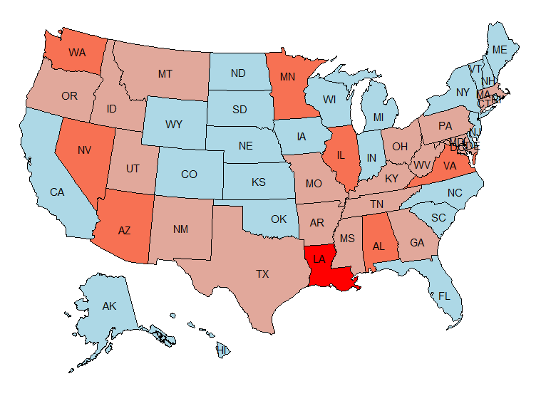
We further relate the clusters to observable state characteristics in order to find an economic interpretation. To this end, we consider five variables: (1) the small firms share, (2) the employment share of manufacturing, (3) the employment share of finance industry, (4) the GDP share of oil production, and (5) the fraction of long-term unemployment on total unemployment. The first four characteristics are considered in Hamilton and Owyang 2012 as possible explanations for heterogeneous regional business cycles.xxxx xx Following this study, we also analyze the clusters based on these attributes. The state-level data of four variables are from Hamilton and Owyang 2012. We also include the share of long-term unemployment, a component that is likely to reflect the structural unemployment.xxixxi xxi The fraction is calculated based on the micro data from the Current Population Survey (CPS). The unemployment rate of a state where the share of long-term unemployment is high might be less responsive to changes in labor demand.
We find that the four clusters are moderately distinct in these five observable dimensions. Table 9 and Figure 3 summarize the observable features of each cluster. The feature of each cluster is computed from the fraction of states in the cluster whose particular observable characteristic is more prominent than the average of all states. For example, according to the second column of Table 8, the fraction of states in cluster 1 whose small firms share is larger than the average of all states is 0.54, and that in cluster 2 is 0.26.
| Small-firm | Manufacturing | Finance | Oil- | Long-term | |
| share | intensive | intensive | producing | unemployment | |
| Cluster 1 | 0.54 | 0.46 | 0.46 | 0.17 | 0.38 |
| Cluster 2 | 0.26 | 0.53 | 0.37 | 0.26 | 0.63 |
| Cluster 3 | 0.14 | 0.43 | 0.43 | 0 | 0.43 |
| Cluster 4 | 1 | 0 | 0 | 1 | 0 |
- •
Numbers in red are larger than 0.5; those in blue are between 0.4 and 0.5.

Cluster 1 is summarily described as small-firm/manufacturing/finance intensive. More than half of the states in this cluster have the share of small firms higher than the average of all states. At the same time, a little less than a half of the states in this cluster have above average employment share of manufacturing.
Cluster 2 is characterized as long-term-unemployment prone and manufacturing intensive. About 60% of states in this cluster have a higher than average share of long-term unemployment, and a little more than half of the states have manufacturing shares in employment above the average.
Cluster 3 is characterized as manufacturing-finance intensive and long-term unemployment prone. Three out of seven states have larger than average fraction of employment in manufacturing and finance. In addition, the three states have above-average long-term unemployment shares.
Louisiana (cluster 4) is an oil-producing state, whose share of small firms is larger than average.
Summing up, clusters are heterogeneous in multiple dimensions, characterized by differences in several observable attributes, as shown in Figure 3. In synthesis, the empirical application demonstrates that our algorithm is be able to reveal meaningful heterogeneity in labor-market dynamics across states without requiring prior knowledge, which in many cases derives from data limitations or from theories lacking empirical support.
5 Conclusion
This paper proposed a new clustering method in a panel MIDAS setting, grouping subjects with similar MIDAS coefficients. The clustering is based on penalized regression approach that is purely data-driven. The major advantage of our method is that it does not require prior knowledge of true group membership, not even of the number of groups. A penalized regression already requires at least two tuning parameters, which are often difficult to choose. A strategy for choosing these tuning parameter are proposed based on a convex region approach. We show that our proposed clustering method works well both asymptotically and in finite samples. The proposed clustering algorithm shines the most when it is combined with our linearized MIDAS model based on Fourier flexible form and polynomials. This novel linearized MIDAS model is simple, accurate, and computationally fast, making it suitable to use with the proposed clustering algorithm for mixed frequency panel data. As an empirical example, we provide an application to labor market dynamics at state level in the United States. The application, based on a mixed frequency Okun’s law model, allows grouping the states in four meaningful clusters that correspond to relevant and measurable differences along different dimensions.
References
- Andreou et al. [2010] E. Andreou, E. Ghysels, and A. Kourtellos. Regression models with mixed sampling frequencies. Journal of Econometrics, 158:246–261, 2010.
- Becker et al. [2004] R. Becker, W. Enders, and S. Hurn. A general test for time dependence in parameters. Journal of Applied Econometrics, 19(7):899–906, 2004.
- Becker et al. [2006] R. Becker, W. Enders, and J. Lee. A stationarity test in the presence of an unknown number of smooth breaks. Journal of Time Series Analysis, 27(3):381–409, 2006.
- Boyd et al. [2011] S. Boyd, N. Parikh, E. Chu, B. Peleato, J. Eckstein, et al. Distributed optimization and statistical learning via the alternating direction method of multipliers. Foundations and Trends® in Machine learning, 3(1):1–122, 2011.
- Breheny and Huang [2011] P. Breheny and J. Huang. Coordinate descent algorithms for nonconvex penalized regression, with applications to biological feature selection. The Annals of Applied Statistics, 5(1):232–253, 2011.
- Breitung and Roling [2015] J. Breitung and C. Roling. Forecasting inflation rates using daily data: A nonparametric midas approach. Journal of Forecasting, 34(7):588–603, 2015.
- Enders and Lee [2012] W. Enders and J. Lee. A unit root test using a fourier series to approximate smooth breaks. Oxford Bulletin of Economics and Statistics, 74(4):574–599, 2012.
- Fan and Li [2001] J. Fan and R. Li. Variable selection via nonconcave penalized likelihood and its oracle properties. Journal of the American Statistical Association, 96(456):1348–1360, 2001.
- Gallant [1981] A. R. Gallant. On the bias in flexible functional forms and an essentially unbiased form: the fourier flexible form. Journal of Econometrics, 15(2):211–245, 1981.
- Ghysels et al. [2007] E. Ghysels, A. Sinko, and R. Valkanov. Midas regressions: Further results and new directions. Econometric Reviews, 26(1):53–90, 2007.
- Güriş [2017] B. Güriş. A New Nonlinear Unit Root Test with Fourier Function. MPRA Paper 82260, University Library of Munich, Germany, Oct. 2017.
- Hamilton and Owyang [2012] J. D. Hamilton and M. T. Owyang. The propagation of regional recessions. Review of Economics and Statistics, 94(4):935–947, 2012.
- Hsu et al. [2012] D. Hsu, S. Kakade, and T. Zhang. A tail inequality for quadratic forms of subgaussian random vectors. Electron. Commun. Probab., 17:1–6, 2012. doi: 10.1214/ECP.v17-2079.
- Hubert and Arabie [1985] L. Hubert and P. Arabie. Comparing partitions. Journal of Classification, 2(1):193–218, 1985.
- Jaccard [1912] P. Jaccard. The distribution of the flora in the alpine zone. 1. New phytologist, 11(2):37–50, 1912.
- Kargı [2016] B. Kargı. Okun’s law and long term co-integration analysis for oecd countries (1987-2012). EMAJ: Emerging Markets Journal, 6(1), 2016.
- Knotek II [2007] E. S. Knotek II. How useful is okun’s law? Economic Review-Federal Reserve Bank of Kansas City, 92(4):73, 2007.
- Langville and Stewart [2004] A. N. Langville and W. J. Stewart. The kronecker product and stochastic automata networks. Journal of Computational and Applied Mathematics, 167(2):429 – 447, 2004. ISSN 0377-0427.
- Lee [2000] J. Lee. The robustness of okun’s law: Evidence from oecd countries. Journal of macroeconomics, 22(2):331–356, 2000.
- Lv et al. [2019] Y. Lv, X. Zhu, Z. Zhu, and A. Qu. Nonparametric cluster analysis on multiple outcomes of longitudinal data. Statistica Sinica, page Accepted, 2019.
- Ma and Huang [2017] S. Ma and J. Huang. A concave pairwise fusion approach to subgroup analysis. Journal of the American Statistical Association, 112(517):410–423, 2017.
- Ma et al. [2019] S. Ma, J. Huang, Z. Zhang, and M. Liu. Exploration of heterogeneous treatment effects via concave fusion. The international journal of biostatistics, 16(1), 2019.
- Moazzami and Dadgostar [2011] B. Moazzami and B. Dadgostar. Okun’s law revisited: evidence from oecd countries. Int. Bus. Econ. Res. J., 8:21–24, 02 2011. doi: 10.19030/iber.v8i8.3156.
- Perron et al. [2017] P. Perron, M. Shintani, and T. Yabu. Testing for flexible nonlinear trends with an integrated or stationary noise component. Oxford Bulletin of Economics and Statistics, 79(5):822–850, 2017.
- Rand [1971] W. M. Rand. Objective criteria for the evaluation of clustering methods. Journal of the American Statistical Association, 66(336):846–850, 1971.
- Rodrigues and Robert Taylor [2012] P. M. M. Rodrigues and A. M. Robert Taylor. The flexible fourier form and local generalised least squares de-trended unit root tests. Oxford Bulletin of Economics and Statistics, 74(5):736–759, 2012.
- Su et al. [2016] L. Su, Z. Shi, and P. C. B. Phillips. Identifying latent structures in panel data. Econometrica, 84(6):2215–2264, 2016.
- Wang et al. [2018, Forthcoming] H. Wang, Z. Shi, and C.-S. Leung. Admm-mcp framework for sparse recovery with global convergence. IEEE Transactions on Signal Processing, Sep 2018, Forthcoming.
- Zhang [2010] C. Zhang. Nearly unbiased variable selection under minimax concave penalty. Ann. Statist., 38(2):894–942, 04 2010.
- Zhu and Qu [2018] X. Zhu and A. Qu. Cluster analysis of longitudinal profiles with subgroups. Electronic Journal of Statistics, 12:171–193, 01 2018.
Supplementary Material to “Revealing Cluster Structures Based on Mixed Sampling Frequencies”
Yeonwoo Rho1*00 0 *Address of correspondence: Yeonwoo Rho, Department of Mathematical Sciences, Michigan Technological University, Houghton, MI 49931, USA. (yrho@mtu.edu) , Yun Liu2, and Hie Joo Ahn300 0 Emails: Y. Rho (yrho@mtu.edu), Y. Liu (AnnaLiu@quickenloans.com), and H. J. Ahn (HieJoo.Ahn@frb.gov)
1Michigan Technological University
2Quicken Loans
3Federal Reserve Board
August 11, 2026
This supplementary material consists of two parts: Section A consists of details of algorithms used in the main paper; and Section B presents all proofs.
Appendix A Algorithms
This section contains details of algorithms introduced in the main paper. Section A.1 introduce details of B&R’s nonparametric MIDAS in our setting in Section 2. Section A.2 present our clustering algorithm (F-clust). Details on how to solve the optimization problem in (12) in our setting is presented using the alternating direction method of multipliers (ADMM) algorithm. The proposed algorithm is also shown to be convergent. Sections A.3 and A.4 present the details of the two competing clustering methods. In particular, Section A.3 introduces how to combine the penalized regression approach with objective function (12) and the B&R’s method (B&R-clust). Section A.4 present the algorithm combining Su’s penalty function and the Fourier transformation for MIDAS (Fourier-Su). Section A.5 presents the algorithm to exclude a part of parameters from clustering.
A.1 Breitung and Roling 2015’s Nonparametric MIDAS
The nonparametric MIDAS in Breitung and Roling 2015 is based on the discrete form of the cubic smooth spline. The least-squares objective function is penalized by the sum of the second difference of weights to balance the goodness of fit and the smoothness of weights. Assume that the MIDAS model is shown in (1). The penalized least-squares objective function is
where indicates the second difference of weights. The smoothed least-squares (SLS) estimator [Breitung and Roling 2015] becomes
where
The tuning parameter can be chosen using an information criteria. For example, Breitung and Roling 2015 proposed to use the modified Akaike information criterion (AIC),
where .
A.2 Clustering algorithm for the Fourier Transformed data
The optimization problem in (12) is not trivial. The alternating direction method of multipliers (ADMM) algorithm by Boyd et al. 2011 has been successfully employed solving this optimization problem [Ma and Huang 2017, Zhu and Qu 2018]. This section introduces the ADMM algorithm in our setting and proves that it is convergent.
By introducing , minimizing (12) is equivalent to minimizing
where . Following Boyd et al. 2011, this constrained optimization problem can be solved using a variant of the augmented Lagrangian
| (S.1) |
where and are -vectors of Lagrangian multipliers. As proposed by Boyd et al. 2011, the optimization problem in (S.1) can be solved using the alternating direction method of multipliers (ADMM) algorithm. At the -th step of the ADMM algorithm, estimated parameters and are updated as
| (S.2) | ||||
where and are the estimates in the -th iteration. By collecting terms related to , the first function in (S.2) is equivalent to minimizing
where , , is an -dimension vector with the -th element as one and the rest as zeros, and is an identity matrix with rank . Therefore, .
The MCP is shown to be nearly unbiased and is applicable here to update [Zhu and Qu 2018]. The penalty function of MCP is where . As a consequence, when the MCP is selected, can be updated by
where and for the global convexity of the second minimization function in (S.2) [Wang et al. 2018, Forthcoming].
If the minimization function of is non-convex, assigning appropriate initial values becomes essential. A proper start will lead to an ideal solution. Inspired by Zhu and Qu 2018, the clustering method can be initialized as shown in the following algorithm.
The estimated number of groups, , can be obtained by . If , and are expected to be in the same cluster. However, as a penalty has been imposed in the clustering algorithm, the equality of two estimated parameters is not achievable. As a result, the MCP penalty is utilized on . Two parameters and are clustered in the same group if .
In Algorithm 1, the stopping criteria are defined as the following. Let , and , . At any step , if for some small values and , and , the algorithm stops. Following Zhu and Qu 2018, define and as
where , indicates the cardinality of . Here, and are predetermined small values.
Proposition 1.
The above clustering algorithm ensures convergence, that is, as .
Proof of Proposition 1.
can be shown similarly to the proof of Proposition 1 in Ma and Huang 2017. The proof of can be done by ignoring the penalty term in the objective function in the proof of Theorem 3.1 in Zhu and Qu 2018. ∎
Proposition 1 demonstrates that the clustering algorithm is convergent as the number of iteration, , approaches infinity. The stopping criteria can be satisfied at some step eventually.
A.3 Comparable Clustering Methods 1: B&R-clust
Recall that in (9), the MIDAS regression model without Fourier transformation of each subject is
For more than one subject, the penal MIDAS model can be written as
where is the raw observations, , .
Refer to the main idea of Breitung and Roling 2015, the cubic smoothing spline penalty is considered. The penalized objective function will be given as
where is the pre-determined smoothing parameter, . is defined as
According to Zhu and Qu 2018, our goal is to solve the constrained optimization function
| (S.3) |
Note that Algorithm 2 follows the same main idea of Zhu and Qu 2018. However, in Zhu and Qu 2018, the model introduces B-splines to approximate observations, while Algorithm 2 simply uses all high-frequency regressors. Moreover, an additional tuning parameter, , is required to be predetermined. Refer to Breitung and Roling 2015, Zhu and Qu 2018, the selection of is based on the minimum of AIC given by
where . The selection of here, is by minimizing
With fixed , can be obtained for different values of . Then, fix with minimum BIC, can be calculated based on the determined .
A.4 Comparable Clustering Methods 2: Fourier-SSP
Su et al. 2016 introduced C-Lasso for clusters to identify relatively large differences between parameters and group averages rather than the traditional Lasso for each subject to select relevant covariates. The penalized profile likelihood (PPL) function mentioned in Su et al. 2016 is
By introducing the group Lasso penalty, the PPL criterion function becomes
where is a tuning parameter. The C-Lasso estimation and , respectively. Without any prior knowledge of the true clusters, PPL C-Lasso estimation requires a predetermination of a reasonable maximum value, , of groups. An appropriate choice of can be found by minimizing IC based on all possible values of clusters less than as long as predetermined values of . To start the algorithm, Su et al. 2016 suggested a natural initial value as for all and as the quasi-maximum likelihood estimation (QMLE) of in each subjects. More details can be found in Su et al. 2016.
Su et al. 2016 provided a stopping criteria for this algorithm:
where is a predetermined small value indicating the tolerance level.
A.5 Algorithm for dropping a part of regressors in clustering
In the framework shown in Section 3, the procedure concentrates on clustering weights of and at the same time. To cluster part of weights, a selection matrix is introducedxxiixxii xxii Although we do not provide a formal proof for this argument, the validity of this algorithm can be proved in a similar manner, following Ma et al. 2019’s argument. To keep the paper concise, we do not present the detail in this paper.. The modified penalized objective function:
where is a matrix of 1s and 0s that picks up the coefficient of interest. For example, if one is interested in clustering Fourier transformed weights only, the matrix is the same as in (4). The group-specified parameter is , and the constrained optimization problem is
Equivalently,
where and . The corresponding algorithm can be summarized as Algorithm 4.
Appendix B Proofs
B.1 Lemmas
Assumptions on regressors (in our setting, ) made in Ma et al. 2019 and related papers can be somewhat too strong for our panel setting. For example, (C3) in Ma et al. 2019 assumes that each column of , taking only the rows that correspond to the -th group, should be nonrandom, and the sum of squares of all its elements is assumed to be equal to the size of -th group, i.e., . This type of assumption could be realistic for data involved with an experimental design, but not suitable for panel data setting, where columns of generally consists of random variables. In this proof, we circumvent this issue by using the following lemmas.
Lemma 1.
Proof of Lemma 1.
When , this lemma is a special case of Theorem 2.1 in Hsu et al. 2012. This can be easily seen by recognizing their , , and are , , and , respectively.
If , a similar argument can still be used. Consider a singular value decomposition of , where and are and orthogonal matrices, respectively. Let denote the nonzero eigenvalues of and . is an matrix, where its diagonal elements are equal to for and all other entries are zero. Let be a vector of independent standard Gaussian random variables. Since is orthogonal, is also an vector of independent standard Gaussian random variables. Let . Applying Lemma 2.4 of Hsu et al. 2012 on then
| (S.4) |
for any . For any and , using similar arguments as in (2.3) and (2.4) of Hsu et al. 2012, Assumption 4, and (S.4),
Let ), , and . The desired proof is concluded by using similar arguments as Hsu et al. 2012 and observing , , and .
A similar proof works for . In this case, without loss of generality, the only nonzero element in are the first diagonal elements of . Let , , be the nonzero diagonal elements of . Then , where are independent standard Gaussian random variables. The rest of the proof is the same. ∎
Lemma 2.
Proof of Lemma 2.
Fix a matrix that satisfies Assumption 2. Using Lemma 1, for any ,
Since is the maximum eigenvalue of , using the fact that is symmetric and positive definite with rank , it can be easily seen that ,
Therefore
Similarly, ,
Therefore for any ,
As a result, given any matrix , the inequalities in the statement have been validated. ∎
Lemma 3.
Proof of Lemma 3.
Using the law of iterated expectations,
Since and as all elements of in (3) smaller than 1 in magnitude,
hold with probability at least for any defined in Assumption 2. Therefore, with probability at most ,
Since and
Since is bounded in probability, for any , there exists some such that . Therefore
and where .
Without loss of generality, let for a large constant and for small positive constant , then . Take , then . For large enough , is negligible. Similarly, in can be found as the following.
A straightforward calculation derives that
It follows that, with probability ,
and therefore,
For any , there exists some , such that , then
Therefore, where . Similarly, take , then . ∎
B.2 Convergence of the Oracle Estimator
Proof of Theorem 1.
The definition of and lead to
where for any ,
Assumption 2 implies that
so that
| (S.5) |
For all -norms, holds (for example, see p. 433 of Langville and Stewart 2004),
| (S.6) |
Lemma 3, equations (S.5) and (S.6), and the triangle inequality imply that for any ,
with probability at least . Therefore,
| (S.7) |
where is defined in Lemma 3. Therefore, with probability at least ,
This proves the first part of Theorem 1. The remaining proof is for the asymptotic normality of . Let be a matrix, where is the -th row of the matrix , . Then, for any with ,
Since is assumed to be an i.i.d. subgaussian distributed sequence with mean 0 and variance proxy , then . Hence,
Suppose that Assumption 2 and 4 hold where and , then
Moreover, for any , applying Cauchy-Schwarz inequality,
| (S.8) | ||||
The first term can be derived as
For any matrix , . Since for , then
According to Assumption 2, is bounded and let the upper bound be some constant , then . Following 2, ,
Then, by Chebyshev’s inequality, the second term of (S.8) can be derived as
| (S.9) |
where
then, (S.9) becomes
Therefore, the following inequality can be derived.
| (S.10) | ||||
Suppose that , then (S.10) further implies that
By the Lindeberg-Feller Central Limit Theorem, ∎
Proof of Corollary 1.
In the following proof, let and be fixed for simplification. It further indicates that is fixed. Let , (S.7) can be simplified as
The rest of the proof suggests a large enough for each situation that allows and to approach infinity. We often use these somewhat trivial inequalities and in the following proofs, particularly when .
- 1.
Consider with fixed. Let and . Since , then . Therefore,
where , which is free of .
- 2.
Consider with fixed.
- (a)
Consider .
- i.
When is fixed, then . For some constant , let , and , then
where , which is free of .
- ii.
When , for some constant , let , and , then . Since , then
where , which is free of and .
- i.
- (b)
Consider . Let for some , and , then . Therefore,
where , which is free of .
- (a)
- 3.
Consider .
- (a)
Consider ,
- i.
When is fixed, then . Let for some positive constant and , , then
where .
- ii.
When , for some positive constant , let and , and , then . Since , then
where , which is freen of and .
- i.
- (b)
Consider . Let for some constant , and , then . Since ,
where , which is free from and .
- (a)
Combining items 2 and 3 above, we can summarize the choice of as follows:
- Case 1.
The number is fixed. Let as ;
- Case 2.
The number . Whether is fixed or ,
- (a)
when is fixed, and for some constant . Let approaching infinity;
- (b)
when ,
- i.
suppose for some constant . Let approaching infinity;
- ii.
suppose for some constant . Let approaching infinity.
- i.
- (a)
∎
B.3 Convergence of the Calculated Estimator ()
Proof of Theorem 2.
This can be done similarly to the proof of Theorem 4.2 in Ma et al. 2019.
Define and the scaled penalty function as . Let the least-squares objective function and the penalty function be
| (S.11) | ||||
Let and define
-
. The -th vector component of equals to the common value of for .
-
. , which implies the average of each cluster vectors.
It results in that if . Hence, for every , , and for every , . Hence,
| (S.12) |
Theorem 1 results in that for some ,
there exists an event in which , such that . Consider the neighborhood of the true parameter ,
It implies that on the event . For any , let , then which implies that is a vector with duplicated group average of . Through two steps as the following, the statement can be proved that with probability approximating to 1, is a strictly local minimizer of .
- i.
In , for any and . This indicates that the oracle estimator is the minimizer over all duplicated group average .
- ii.
There exists an event such that for large enough , . In , there exists a neighborhood of such that for all for sufficiently large . It means that for all , the duplicated group average is the minimizer.
Then, it results in for any and in . Hence, over , for large enough and , is a strictly local minimizer of with the probability .
First, show for any , where is a constant which does not depend on . It implies that when is close enough to the true parameter , the penalty term would not affect the objective function with respect to different values of . Let . Consider the triangle inequality . Since , then
| (S.13) | ||||
Since , then for all and ,
for some . Then by Assumption 6, is a constant, and furthermore, is a constant. Therefore, , and for all . Since is the unique global minimizer of , then for all and hence for all . By the property of the clustering algorithm, for the -th group, , which implies that, along with the definition of operation , equals to the -th component of for all . Then, by (S.12),
Furthermore, . Therefore, for all .
Second, for a positive sequence , let . For any , by the first order Taylor’s expansion,
and let and . Since
we have
Let for some constant . Then,
| (S.14) | ||||
Consider separating into two parts, , and , for . When , since , then . Thus, the RHS of (S.14) becomes
| (S.15) | ||||
Furthermore, by (S.13), for any , , and therefore, for all , . This lead to
| (S.16) |
where the inequality in (S.16) is obtained by (S.13). Since , by the triangle inequality,
Hence, for , , ,
Since is constant for all , then . Therefore, following for , (S.15) becomes
Furthermore, similarly to (S.13), for all , , Then, since ,
Hence, , because is nondecreasing and concave as assumed in Assumption 3. Then,
| (S.17) |
Let , then
| (S.18) |
In addition, and then,
where . By Lemma 3, , where , , and given in Assumption 2 and 4. is defined in Lemma 3. Then, over the event ,
| (S.19) |
Therefore, by (S.17), (S.18) and (S.19),
where and .
Let , then . Suppose that the following condition is true over the event ,
| (S.20) |
then . Once (S.20) holds, with probability approaching to 1 as .
Note that can be chosen as any sequence of numbers, as long as to ensure . In the following argument, conditions on , , , and other numbers that satisfies (S.20) are spelled out:
- 1.
As with fixed, the proposed estimator does not converge to the oracle estimator.
- 2.
- 3-1.
Let . Consider the first part of (S.20). Choose such that and as . Let . Then
- 3-2.
Let . Consider the second part of (S.20).
- (a)
Suppose is fixed. Choose such that and as . Let for some positive constant . Then, , and
where .
- (b)
Suppose . Choose such that and as . Let . Then, and . Further, since ,
where , which is free from and .
- (c)
Suppose . Let for a positive constant . Choose such that and . Then, . Since ,
where , which is free of and .
- (a)
Combining the above calculations and the proof of Corollary 1, the conditions for (S.20) can be summarized as follows:
∎
References
- Andreou et al. [2010] E. Andreou, E. Ghysels, and A. Kourtellos. Regression models with mixed sampling frequencies. Journal of Econometrics, 158:246–261, 2010.
- Becker et al. [2004] R. Becker, W. Enders, and S. Hurn. A general test for time dependence in parameters. Journal of Applied Econometrics, 19(7):899–906, 2004.
- Becker et al. [2006] R. Becker, W. Enders, and J. Lee. A stationarity test in the presence of an unknown number of smooth breaks. Journal of Time Series Analysis, 27(3):381–409, 2006.
- Boyd et al. [2011] S. Boyd, N. Parikh, E. Chu, B. Peleato, J. Eckstein, et al. Distributed optimization and statistical learning via the alternating direction method of multipliers. Foundations and Trends® in Machine learning, 3(1):1–122, 2011.
- Breheny and Huang [2011] P. Breheny and J. Huang. Coordinate descent algorithms for nonconvex penalized regression, with applications to biological feature selection. The Annals of Applied Statistics, 5(1):232–253, 2011.
- Breitung and Roling [2015] J. Breitung and C. Roling. Forecasting inflation rates using daily data: A nonparametric midas approach. Journal of Forecasting, 34(7):588–603, 2015.
- Enders and Lee [2012] W. Enders and J. Lee. A unit root test using a fourier series to approximate smooth breaks. Oxford Bulletin of Economics and Statistics, 74(4):574–599, 2012.
- Fan and Li [2001] J. Fan and R. Li. Variable selection via nonconcave penalized likelihood and its oracle properties. Journal of the American Statistical Association, 96(456):1348–1360, 2001.
- Gallant [1981] A. R. Gallant. On the bias in flexible functional forms and an essentially unbiased form: the fourier flexible form. Journal of Econometrics, 15(2):211–245, 1981.
- Ghysels et al. [2007] E. Ghysels, A. Sinko, and R. Valkanov. Midas regressions: Further results and new directions. Econometric Reviews, 26(1):53–90, 2007.
- Güriş [2017] B. Güriş. A New Nonlinear Unit Root Test with Fourier Function. MPRA Paper 82260, University Library of Munich, Germany, Oct. 2017.
- Hamilton and Owyang [2012] J. D. Hamilton and M. T. Owyang. The propagation of regional recessions. Review of Economics and Statistics, 94(4):935–947, 2012.
- Hsu et al. [2012] D. Hsu, S. Kakade, and T. Zhang. A tail inequality for quadratic forms of subgaussian random vectors. Electron. Commun. Probab., 17:1–6, 2012. doi: 10.1214/ECP.v17-2079.
- Hubert and Arabie [1985] L. Hubert and P. Arabie. Comparing partitions. Journal of Classification, 2(1):193–218, 1985.
- Jaccard [1912] P. Jaccard. The distribution of the flora in the alpine zone. 1. New phytologist, 11(2):37–50, 1912.
- Kargı [2016] B. Kargı. Okun’s law and long term co-integration analysis for oecd countries (1987-2012). EMAJ: Emerging Markets Journal, 6(1), 2016.
- Knotek II [2007] E. S. Knotek II. How useful is okun’s law? Economic Review-Federal Reserve Bank of Kansas City, 92(4):73, 2007.
- Langville and Stewart [2004] A. N. Langville and W. J. Stewart. The kronecker product and stochastic automata networks. Journal of Computational and Applied Mathematics, 167(2):429 – 447, 2004. ISSN 0377-0427.
- Lee [2000] J. Lee. The robustness of okun’s law: Evidence from oecd countries. Journal of macroeconomics, 22(2):331–356, 2000.
- Lv et al. [2019] Y. Lv, X. Zhu, Z. Zhu, and A. Qu. Nonparametric cluster analysis on multiple outcomes of longitudinal data. Statistica Sinica, page Accepted, 2019.
- Ma and Huang [2017] S. Ma and J. Huang. A concave pairwise fusion approach to subgroup analysis. Journal of the American Statistical Association, 112(517):410–423, 2017.
- Ma et al. [2019] S. Ma, J. Huang, Z. Zhang, and M. Liu. Exploration of heterogeneous treatment effects via concave fusion. The international journal of biostatistics, 16(1), 2019.
- Moazzami and Dadgostar [2011] B. Moazzami and B. Dadgostar. Okun’s law revisited: evidence from oecd countries. Int. Bus. Econ. Res. J., 8:21–24, 02 2011. doi: 10.19030/iber.v8i8.3156.
- Perron et al. [2017] P. Perron, M. Shintani, and T. Yabu. Testing for flexible nonlinear trends with an integrated or stationary noise component. Oxford Bulletin of Economics and Statistics, 79(5):822–850, 2017.
- Rand [1971] W. M. Rand. Objective criteria for the evaluation of clustering methods. Journal of the American Statistical Association, 66(336):846–850, 1971.
- Rodrigues and Robert Taylor [2012] P. M. M. Rodrigues and A. M. Robert Taylor. The flexible fourier form and local generalised least squares de-trended unit root tests. Oxford Bulletin of Economics and Statistics, 74(5):736–759, 2012.
- Su et al. [2016] L. Su, Z. Shi, and P. C. B. Phillips. Identifying latent structures in panel data. Econometrica, 84(6):2215–2264, 2016.
- Wang et al. [2018, Forthcoming] H. Wang, Z. Shi, and C.-S. Leung. Admm-mcp framework for sparse recovery with global convergence. IEEE Transactions on Signal Processing, Sep 2018, Forthcoming.
- Zhang [2010] C. Zhang. Nearly unbiased variable selection under minimax concave penalty. Ann. Statist., 38(2):894–942, 04 2010.
- Zhu and Qu [2018] X. Zhu and A. Qu. Cluster analysis of longitudinal profiles with subgroups. Electronic Journal of Statistics, 12:171–193, 01 2018.