SPARSE aNETT FOR SOLVING INVERSE PROBLEMS WITH DEEP LEARNING

Throughout this section we assume the following.

• •

  $\mathbf{K}\colon\mathbb{X}\to\mathbb{Y}$ is linear and bounded.

• •

  $\mathbf{E}\colon\mathbb{X}\to\ell^{2}(\Lambda)$ is weakly sequentially continuous.

• •

  $\mathbf{D}\colon\ell^{2}(\Lambda)\to\mathbb{X}$ is weakly sequentially continuous.

• •

  $q\geq 1$, $c>0$,

• •

  $w_{\rm min}\triangleq\inf\{w_{\lambda}\mid\lambda\in\Lambda\}>0$.

Furthermore, we define $\mathbf{N}\triangleq\mathbf{D}\circ\mathbf{E}$ and choose the regularizer

Under these assumptions, (1.2) has a minimizer for all $y\in\mathbb{Y}$ and all $\alpha>0$. Moreover, we have the following results.

Proofs of Theorems 2.1 and 2.2 are given in [10].

First, an autoencoder $\mathbf{N}^{a}$ is trained such that $u$ is close to $\mathbf{N}^{a}(u)$ and that $\lVert\mathbf{E}(u)\rVert_{1,w}$ is small for any $u$ in a class $\mathcal{M}$ of images of interest. For that purpose, we add the regularizer $\lVert\,\cdot\,\rVert_{1,w}$ to the loss function for training $\mathbf{N}^{a}$ as denoising network. To be more specific, let $(\mathbf{N}_{\theta}^{a})_{\theta\in\Theta}$ be a family of autoencoder networks $\mathbf{N}_{\theta}^{a}=\mathbf{D}_{\theta}^{a}\circ\mathbf{E}_{\theta}$, where $\mathbf{E}_{\theta}\colon\mathbb{X}\to\ell^{2}(\Lambda)$ are admissible (in the sense of above assumptions) encoder networks and $\mathbf{D}_{\theta}^{a}\colon\ell^{2}(\Lambda)\to\mathbb{X}$ admissible decoder networks. Moreover, suppose that $u_{1},\dots,u_{m}\in\mathcal{M}$ is a training dataset. To select the particular autoencoder based on the training data, we consider the following training strategy for the sparse denoising autoencoder

and set $[\mathbf{N}^{a},\mathbf{E}]\triangleq[\mathbf{N}_{\theta^{*}}^{a},\mathbf{E}_{\theta^{*}}]$. Here $v_{i}\in\mathbb{X}$ are data perturbations and $\beta>0$ a regularization parameter.

By training with perturbed data points $u_{i}+\varepsilon_{i}$, we increase robustness of the trained autoencoder. Note that the perturbations $\varepsilon_{i}\in\mathbb{X}$ are chosen independently of the operator $\mathbf{K}$ such that the autoencoder can be used for each forward operator in a universal manner. Clearly then, the autoencoder depends on the specific manifold $\mathcal{M}$ of images of interest. As we shall see however, opposed to typical deep learning based reconstruction methods which do not account for data consistency outside the training data set, the sparse aNETT is robust against changes of the specific image manifold. Note that Thms. 2.1 and 2.2 hold true for $\mathbf{N}^{a}$ in place of $\mathbf{N}$.

The sparse aNETT (1.2) consists of a data consistency term, a sparsity term, and an augmented term enforcing $\mathbf{N}(u)\simeq u$. Ideally, the set of all approximately data consistent elements that are also approximate fixed points of $\mathbf{N}$, is close to the image manifold $\mathcal{M}$. However, without adjusting the autoencoder to specific forward models, this is a challenging and maybe impossible task. Indeed, for the application we consider in this paper, namely sparse view CT, we observed that the autoencoder trained independent of the forward operator, was not able to sufficiently well distinguish between data-consistent elements inside and outside desired image class.

One way to increase the value of $\lVert u-\mathbf{N}(u)\rVert$ for undesired but data consistent elements is to adopt the training strategy developed in [7] and to take the data perturbations in (2.1) as $\varepsilon_{i}=\mathbf{K}^{\sharp}\mathbf{K}u_{i}-u_{i}$ where $\mathbf{K}^{\sharp}$ is a reconstruction operator approximating the Moore-Penrose inverse of $\mathbf{K}$, $u_{i}$ are the artifact free images and $\mathbf{K}^{\sharp}\mathbf{K}u_{i}$ images with artefacts. In this case, the training dataset depends on the forward operator, and the autoencoder has to be retrained for every specific forward operator. Therefore, in this paper we follow a different approach. Instead of adjusting the autoencoder training, we compose the operator independent autoencoder $\mathbf{N}^{a}$ with another network $\mathbf{U}$, that is trained to distinguish between the desired images and images with operator dependent artefacts. For that purpose we choose a network architecture $(\mathbf{U}_{\kappa})_{\kappa\in K}$ and select $\mathbf{U}=\mathbf{U}_{\kappa^{*}}$, where $\kappa^{*}$ is a minimizer of

where $v_{i}=\mathbf{K}^{\sharp}\mathbf{K}u_{i}$ for $i=1,\dots,m$ and $v_{i}=u_{i}$ for $i=m+1,\dots,2m$ and $\gamma>0$ is a regularization parameter. We see that Thms. 2.1 and 2.2 still hold true for the final autoencoder $\mathbf{N}\triangleq\mathbf{U}\circ\mathbf{N}^{a}$ if $\mathbf{U}$ is weakly sequentially continuous.

We first train $\mathbf{N}^{a}$, $\mathbf{E}$ by minimizing (2.1) and subsequently train $\mathbf{U}$ by minimizing (2.2). The sparse autoencoder is chosen as $\mathbf{N}=\mathbf{U}\circ\mathbf{N}^{a}$. The network architecture chosen for the problem adapted network $\mathbf{U}$ is the tight frame U-Net [13] and the auto-encoder architecture is chosen as in [14]. The perturbations in (2.1) are taken as independent realizations of Gaussian white noise with standard deviation $p\cdot\bar{u}_{i}$ where $p$ is uniformly sampled from $[0,0.1]$ and $\bar{u}_{i}$ is the mean of $u_{i}$. The weighs in the $\ell^{1}$-term are taken as $w_{\ell(\lambda)}=2^{-\ell}$ where $\ell(\lambda)$ is the index of the downsampling-step, see [14].

We train all networks using the Adam [15] optimizer with the recommended parameters for $100$ iterations and use only the best parameters of these iterations. Here, the best parameters are those which give the smallest loss on the validation set. The parameters $\eta,\beta,\gamma$ are chosen empirically and we found that $\eta=10^{-3}$ and $\beta=\gamma=10^{-5}$ give the best results for our approach.

For minimizing the sparse aNETT functional (1.2) we use a splitting approach. For that purpose we introduce the auxiliary variable $\xi=\mathbf{E}(u)$ and rewrite (1.2) as the following constraint optimization problem

Note that we have only replaced $\mathbf{E}(u)$ in th $\ell^{1}$-term but not in the augmented term. To solve the above constrained version of aNETT, we use the ADMM scheme with scaled dual variable. This results in the update scheme

where $\rho>0$ is a scaling parameter. The strength of the splitting type iteration (3.1)-(3.3) is that the optimization problems involved in each iterative update is simpler and easier to solve than the original sparse aNETT minimization problem (1.2), which contains the non-differentiable $\ell^{1}$-norm as well as non-linear augmented network term. In fact, the $\xi$-update can be explicitly solved by soft-thresholding. Additionally, if we take $\mathbf{N}$ being differentiable, the $u$-update can be solved efficiently using gradient type iterative schemes.

We minimize (3.1) using gradient descent with momentum parameter $0.8$. The ADMM is initialized with $u_{0}=\mathbf{N}(\mathbf{K}^{\sharp}y)$, $\xi_{0}=\mathbf{E}(u_{0})$ and $\eta_{0}=0$, where $y$ are the given data. Here and below $\mathbf{K}^{\sharp}$ denotes the filtered backprojection operator. The parameter specifications for the minimization using (3.1)-(3.3) in various scenarios are shown in Table 3.1. All parameters were chosen empirically to give the best results. Here, outer refers to the total ADMM iterations, stepsize is the stepsize and inner is the maximal number of iterations for the $u$-update step (3.1).

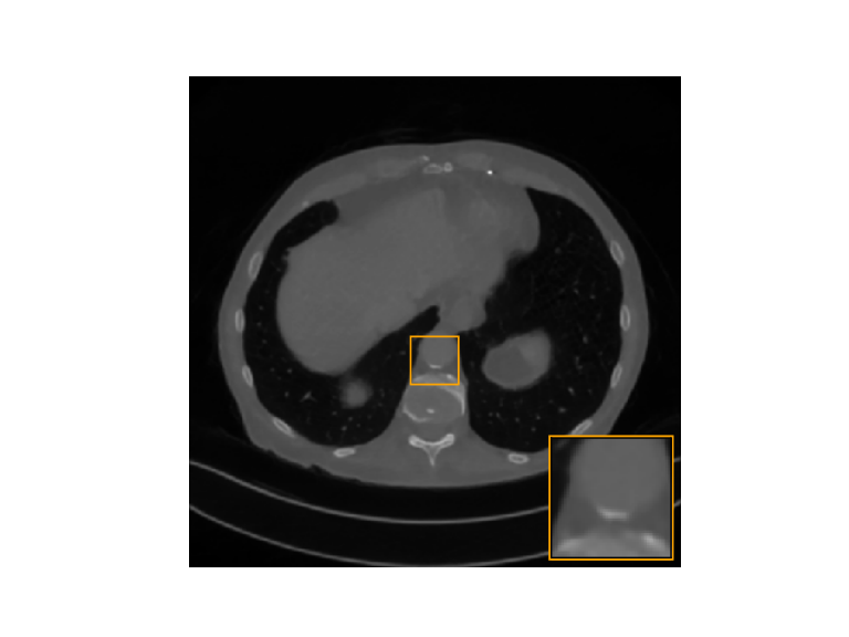
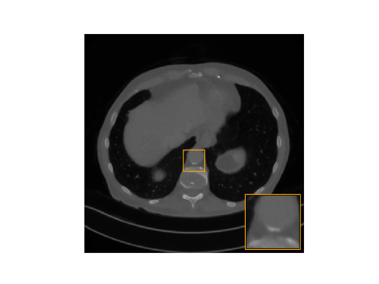
The first case we consider is the case of noise-free data. Figure 3.1 shows the FBP reconstruction $u_{\mathrm{FBP}}=\mathbf{K}^{\sharp}(y)$ and the reconstruction with the full network $u_{\mathrm{post}}=\mathbf{N}(u_{\mathrm{FBP}})$ where $\mathbf{N}$ is defined as above and the aNETT reconstruction $u_{\mathrm{aNETT}}$. Comparing the results we see that the output of the problem adapted network $u_{\mathrm{post}}$ and the aNETT output $u_{\mathrm{aNETT}}$ are visually identical. This is because, the test image $u$ is close to the training data and therefore the considered training procedure implies that $u_{\mathrm{post}}$ is close to minimizer of the sparse aNETT. In comparison to the FBP we see that the aNETT was able to completely remove all the artefacts and yields an almost perfect reconstruction.

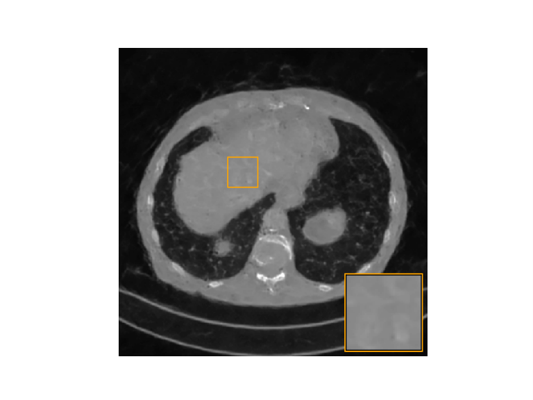
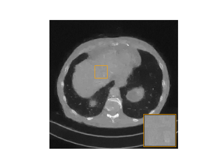
To simulate noisy data we add $5\text{\,}\mathrm{\%}$ Gaussian noise to the measurement data, i.e. we use $y_{\delta}=y+0.05\cdot\bar{y}\cdot\delta$ where $\bar{y}$ is the mean of the data and $\delta$ is a standard normal distributed noise term. Reconstructions using FBP, post-processing and the sparse aNETT are shown in Figure 3.2. We enhance the contrast in these images by a factor of $c=1.7$ using the Python Pillow library [16] to make the differences more clearly visible. The post-processing reconstruction shows some noise-like structure on parts where the image should be mostly constant, e.g. in and around the orange square. We hypothesize that these noise like structures occur because the problem adapted network $\mathbf{U}$ has not been trained with noise in the data domain and hence has difficulties in reconstructing these. While we could add this to the training the networks would then likely fail on different noise models, e.g. Poisson noise. Comparing this to the aNETT we see that this noise-like structure has been greatly reduced and we have to rely more on the sparsifying term of the regularization method to get noise-free reconstructions.

One particular advantage of aNETT over post-processing is the increased robustness with respect to the type of image to be reconstructed. To highlight this advantage, as illustrated in the top left image in Figure 3.3 we add a high intensity disc to the CT image shown in 3.1. The disc represents a clear low complexity structure and its accurate reconstruction should be easily possible.

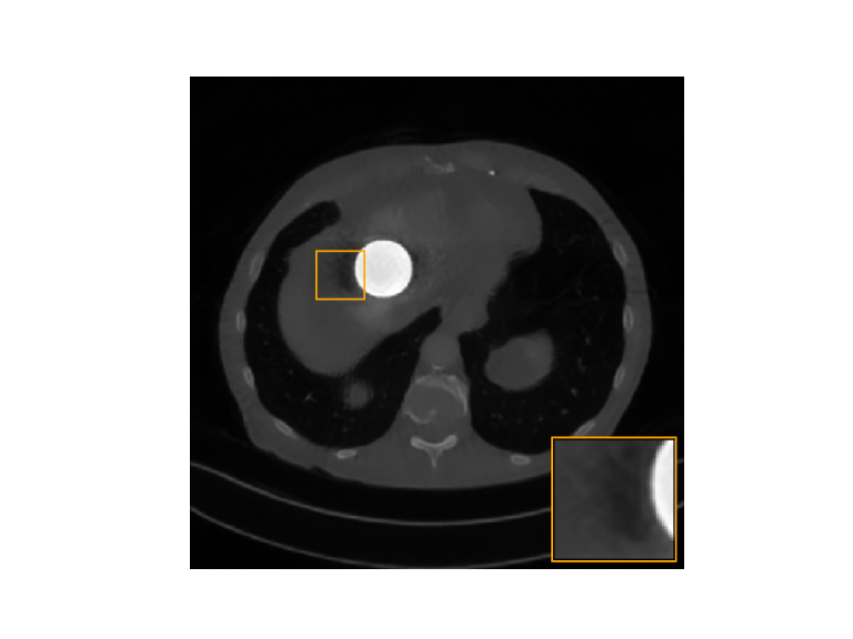
Figure 3.3 shows the reconstructions using the FBP, the post-processing network and the aNETT. Taking a look at the zoomed in square in these images we see that FBP well reconstructs the circle. The post-processing network output, however, has some dark spots close to the circle and generally shows data-inconsistent behaviour around the circle. On the other hand, using the aNETT we see that these problems do not occur. This improved accuracy is because aNETT takes into account the given data even for images different form the training data.

References

- [1] HW Engl, M Hanke, and A Neubauer, Regularization of inverse problems, vol. 375, Springer Science & Business Media, 1996.
- [2] O Scherzer, M Grasmair, H Grossauer, M Haltmeier, and F Lenzen, Variational methods in imaging, Springer, 2009.
- [3] D Lee, J Yoo, and JC Ye, “Deep residual learning for compressed sensing mri,” in 2017 IEEE 14th International Symposium on Biomedical Imaging (ISBI 2017). IEEE, 2017, pp. 15–18.
- [4] KH Jin, M McCann, E Froustey, and M Unser, “Deep convolutional neural network for inverse problems in imaging,” IEEE Trans. Image Process., vol. 26, no. 9, pp. 4509–4522, 2017.
- [5] J Sun, H Li, and Z et al. Xu, “Deep ADMM-Net for compressive sensing MRI,” in Advances in neural information processing systems, 2016, pp. 10–18.
- [6] G Wang, “A perspective on deep imaging,” IEEE Access, vol. 4, pp. 8914–8924, 2016.
- [7] H Li, J Schwab, S Antholzer, and M Haltmeier, “NETT: Solving inverse problems with deep neural networks,” Inverse Probl., 2020.
- [8] M Grasmair, M Haltmeier, and O Scherzer, “Sparse regularization with -penalty term,” Inverse Probl., vol. 24, no. 5, pp. 055020, 2008.
- [9] I Daubechies, M Defrise, and C De Mol, “An iterative thresholding algorithm for linear inverse problems with a sparsity constraint,” Commun. Pur. Appl. Math., vol. 57, no. 11, pp. 1413–1457, 2004.
- [10] M Haltmeier, L Nguyen, D Obmann, and J Schwab, “Sparse -regularization of inverse problems with deep learning,” arXiv:1908.03006, 2019.
- [11] J Adler, H Kohr, and O Öktem, “Operator discretization library (odl),” Software available from https://github. com/odlgroup/odl, 2017.
- [12] C McCollough, “TU-FG-207A-04: Overview of the low dose CT grand challenge,” Med. Phys., vol. 43, no. 6Part35, pp. 3759–3760, 2016.
- [13] Y Han and JC Ye, “Framing u-net via deep convolutional framelets: Application to sparse-view ct,” IEEE Trans. Med. Imag., vol. 37, no. 6, pp. 1418–1429, 2018.
- [14] D Obmann, J Schwab, and M Haltmeier, “Deep synthesis regularization of inverse problems,” arXiv:2002.00155, 2020.
- [15] D Kingma and J Ba, “Adam: A method for stochastic optimization,” arXiv:1412.6980, 2014.
- [16] A Clark, “Pillow (pil fork) documentation,” 2015.
- [17] A Kofler, M Haltmeier, C Kolbitsch, M Kachelrieß, and M Dewey, “A U-Nets cascade for sparse view computed tomography,” in International Workshop on Machine Learning for Medical Image Reconstruction. Springer, 2018, pp. 91–99.
- [18] J Schlemper, J Caballero, J Hajnal, A Price, and D Rueckert, “A deep cascade of convolutional neural networks for dynamic MR image reconstruction,” IEEE Trans. Med. Imag., vol. 37, no. 2, pp. 491–503, 2017.
- [19] J Adler and O Öktem, “Solving ill-posed inverse problems using iterative deep neural networks,” Inverse Probl., vol. 33, no. 12, pp. 124007, 2017.
- [20] E Kobler, T Klatzer, K Hammernik, and T Pock, “Variational networks: connecting variational methods and deep learning,” in German conference on pattern recognition. Springer, 2017, pp. 281–293.
- [21] J Schwab, S Antholzer, and M Haltmeier, “Deep null space learning for inverse problems: convergence analysis and rates,” Inverse Probl., vol. 35, no. 2, pp. 025008, 2019.