A microscopic approach to study the onset of a highly infectious disease spreading
Abstract
We combine a pedestrian dynamics model with a contact tracing method to simulate the initial spreading of a highly infectious airborne disease in a confined environment. We focus on a medium size population (up to 1000 people) with a small number of infectious people (1 or 2) and the rest of the people is divided between immune and susceptible. We adopt a space-continuous model that represents pedestrian dynamics by the forces acting on them, i.e. a microscopic force-based model. Once discretized, the model results in a high-dimensional system of second order ordinary differential equations. Before adding the contact tracing to the pedestrian dynamics model, we calibrate the model parameters, validate the model against empirical data, and show that pedestrian self-organization into lanes can be captured. We consider an explicit approach for contact tracing by introducing a sickness domain around a sick person. A healthy but susceptible person who remains in the sickness domain for a certain amount of time may get infected (with a prescribed probability) and become a so-called secondary contact. As a concrete setting to simulate the onset of disease spreading, we consider terminals in two US airports: Hobby Airport in Houston and the Atlanta International Airport. We consider different scenarios and we quantify the increase in average number of secondary contacts increases as a given terminal becomes more densely populated, the percentage of immune people decreases, the number of primary contacts increases, and areas of high density (such as the boarding buses) are present.
Keywords: Crowd dynamics, contact tracing, disease spreading, complex systems
1 Introduction
The focus of this work is to study the initiation of disease spreading in a confined, yet complex environment (e.g. an airport terminal), and in a medium size population (up to 1000 people) with a small number of infectious people (1 or 2). Standard epidemic theory models describe the evolution of disease spreading in terms of groups that are susceptible to, infected with and recovered from a particular disease. The SIR (Susceptible Infected Recovered - see, e.g., [28, 45]) and SIS (Susceptible Infected Susceptible - see, e.g., [24, 18]) models are the foundation of almost all of mathematical epidemiology. To quantify the transmission dynamics through contact with healthy individuals, these models use the basic reproduction number, which measures the number of infected people (secondary contacts) from an infectious person (primary contact) in a population where all the people are susceptible. Most models predicting the severity of an epidemic estimate the basic reproduction number for large population sizes. See, e.g., [12, 31, 26] and references therein. Such models are typically not valid when the number of infected individuals is small and the size of healthy population is medium. Medium sized population are typical of confined environments like airports and hospital waiting rooms, which are the most likely transmittal places during the initial stage of disease spreading. See, e.g., [37, 38] Understanding contact tracing associated with such environments is of paramount importance for an early suppression of an epidemic.
We propose a simple approach for contact tracing built on a microscopic pedestrian dynamics model. Usually, contact tracing is meant as a disease control strategy in which the people who have been in close contact to infectious persons are traced. These traced people are monitored so that if they become symptomatic they can be efficiently isolated and the disease transmission can be contained [16, 17]. The effectiveness of contact tracing as a control strategy for ebola and tuberculosis have been studied theoretically in, e.g., [44, 19]. Previous works on contact tracing use a wide range of methodologies from individual based models on specific networks to compartmental ordinary differential equations at the population level. See, e.g., [41, 30, 31, 2, 12] and references therein. Many differential equation models incorporate contact tracing implicitly (see, e.g. [40, 44]). In our simulations, contact tracing is limited to pedestrians coming in contact during a short time span (up to 1 hour). The contact tracing method is combined with a pedestrian dynamics model to estimate the number of people that could potentially be infected by a few sick people around them, thereby providing a tool to study the onset of disease spreading.
A very large variety of models have been developed over the years to describe the complex dynamical behavior of pedestrian crowds. The different mathematical models can be divided into three main categories depending on the (macroscopic, mesoscopic, microscopic) scale of observation [8]. Macroscopic models (see, e.g., [25, 48]) are suitable for high density, large-scale systems. Thus, they will not be considered for the proposed work. The mesoscale approach [5, 1, 4, 7, 6, 9, 10, 6, 11, 3, 29] derives a Boltzmann-type evolution equation for the statistical distribution function of the position and velocity of the pedestrians, in a framework close to that of the kinetic theory of gases. Microscopic force-based models, which use Newtonian mechanics to interpret pedestrian movement as the physical interaction between the people and the environment, are one of the most popular modeling paradigms of continuous models because they describe the movement of pedestrians well qualitatively. See, e.g., [20, 22, 23, 50, 39, 14, 55, 33] and references therein. Collective phenomena, like unidirectional or bidirectional flow in a corridor [35, 49, 52], lane formation [22, 21, 53], oscillations at bottlenecks [22, 21], the faster-is-slower effect [32, 42], emergency evacuation from buildings [21, 53, 34], are well reproduced. Other advantages of these methods are the ease of implementation, and in particular parallel implementation, and the fact that they permit higher resolution for geometry and time. Because of these advantages, we choose to build our contact tracing method on a microscopic force-based model first presented in [15].
In most of the references cited above, models have been shown to replicate various cases of pedestrian movement qualitatively through analysis and/or numerical simulations. The quantitative validation of pedestrian flow models is complicated by the lack of reliable experimental data. In addition, the few available datasets show large differences [46, 47, 54]. After a calibration of the model parameters, we validate the model in [15] by comparing with empirical data from [54]. We obtain a good quantitative agreement between the computed and measured fundamental diagrams for a set of 9 experiments, all involving unidirectional motion in a corridor. We run a series of tests to understand self-organized lane formation, as this is relevant to the kind of environment we focus on. Finally, we mention that adjustment of the parameters and data assimilations have also been proposed in [51, 27] to make evolutionary models more reliable.
The validated pedestrian dynamics model is then combined with a simple method to trace contact. One or two sick people, referred to as primary contacts, are introduced in the pedestrian population. The people infected by the primary contact are called secondary contacts. We consider an explicit approach for contact tracing by introducing a sickness domain around a primary contact. A healthy but susceptible person who remains in that sickness domain for a certain amount of time may get infected (with a prescribed probability) and become a secondary contact. As a concrete setting to simulate the onset of disease spreading, we consider terminals in two US airports: Hobby Airport in Houston and the Atlanta International Airport. We consider different scenarios: variable population size, variable percentage of immune (non-susceptible) population, boarding bridges or boarding buses. Through the numerical simulations, we quantify the increase in average number of secondary contacts increases as a given terminal becomes more densely populated, the percentage of immune people decreases, the number of primary contacts increases, and areas of high density (such as the boarding buses) are present.
The outline of this paper is as follows. In Sec. 2, we introduce the force-based microscopic model for pedestrian dynamics we will build upon, we describe the numerical method, calibrate the model parameters and validate the model against experimental data. In Sec. 3, we show that the model is capable of reproducing self-organization of pedestrians. In Sec. 4, we present our contact tracing method and combine it with the pedestrian dynamics model to simulate the initial spreading of a highly infectious airborne disease. We report the average number of people infected by one or two sick people in terminals of Hobby Airport and Atlanta International Airport for different scenarios. Conclusions are drawn in Sec. 5.
2 A microscopic force-based model for pedestrian dyanmics
We briefly present the model we focus on, which was introduced in [15]. Let us consider a group of pedestrians in a bounded geometry . Each pedestrian is modeled as a circular disk with a given radius. The dynamics of each pedestrian over a time interval of interest is modeled using Newton’s second law, i.e. for pedestrian with mass and center of mass at the law of motion is:
| (1) |
where represents the total forces acting on the pedestrian. Source term includes the force driving the pedestrian towards their target and the repulsive forces acting on the pedestrian from other pedestrians, walls, and other obstacles. Finding an appropriate description of to obtain realistic pedestrian motion is not a trivial task.
Given , the boundary is represented as a set of points: with , for . The set of boundary points acting on pedestrian at time is:
where denotes the Euclidean norm in and is a cutoff radius for pedestrian-wall interaction. The set of all pedestrians that influence the motion of pedestrian at a certain time is:
where is a cutoff radius for pedestrian-pedestrian interaction. We assume that the total forces consist of three contributions:
| (2) |
where is the force driving pedestrian to their target, is the repulsive force pedestrian exerts on pedestrian , and is the repulsive force due to the domain boundary. Repulsive forces and model the pedestrians’ attempt to avoid collisions and contact by changing their direction.
The driving force models the intention of a pedestrian to reach a destination with a certain desired speed :
| (3) |
where is the unit vector directed from pedestrian to their target, is the velocity of pedestrian , and is a time constant. To represent more involved paths, we generate a sequence of “checkpoints” along the path and for each checkpoint we specify a radius . Checkpoint is considered to be reached when the pedestrian is within a distance of it. Once a path is assigned to a pedestrian, the target is the first checkpoint along the path and when the first checkpoint is reached the target is updated to the second checkpoint, and so on.
In order to define repulsive force in (2), we need to introduce some notation. The vector connecting pedestrian with pedestrian , directed from to , and the corresponding unit vector are denoted by:
We assume that pedestrian has an effective diameter that depends linearly on their velocity:
| (4) |
being their diameter at rest and being a proportionality parameter. Eq. (4) accounts for the fact that a faster pedestrian has an effective larger diameter since he/she will keep obstacles and other pedestrians at a larger distance. The effective distance between pedestrians and is then:
| (5) |
We can now write the repulsive force as:
| (6) |
where is a parameter used to tune the strength of the force, is the component of the velocity of relative to in the direction of :
and is a coefficient that reduces the action-field of the repulsive force to the angle of vision of each pedestrian (i.e., ):
As is intuitive, repulsive force (6) is directed in the opposite direction of and its modulus is inversely proportional to the effective distance between pedestrians and pedestrian . Moreover, the strength of the repulsive force depends on the angle between and . In fact, the coefficient takes its maximum value (i.e., 1) when pedestrian is moving in the same direction as and it takes its minimum value (i.e., 0) when the angle between and is bigger than . Notice that, thanks to the definition of , pedestrian feels the repulsive force due to pedestrian only if they are moving toward each other. So, e.g., if pedestrian is close to pedestrian , but faster than and ahead of , then . The term at the numerator in eq. (6) prevents collisions when the distance between the two pedestrian is small and the relative speed is low, which would lead to an otherwise small repulsive force. The case corresponds to the centrifugal force model introduced in [53], which is known to lead to realistic results only if supplemented with a collision detection technique. See also [13] for details.
In order to define , we note that the repulsive force between a pedestrian and a wall is zero if is walking parallel to the wall. In the model though, this is not enough to avoid very small repulsive forces when the pedestrians walks almost parallel to the wall. For this reason, we assume that each pedestrian feels the repulsive action of three points lying on the boundary: the closest boundary point to pedestrian denoted by , and the two neighboring points and provided that . If indeed , then , otherwise . We assume that the repulsive force exerted by boundary point on pedestrian is given by:
| (11) |
where is defined in (2), is the component of the velocity normal to the boundary and
2.1 Numerical Method
We introduce the time-discretization step and set , for , with . Moreover, we denote by the approximation of a generic quantity at the time .
Each pedestrian , with , is assigned an initial position and an initial velocity . The position at time , with is found with the following centered finite difference approximation of eq. (1):
| (12) |
where is an approximation of in eq. (2) at time . Notice that for in eq. (12) we need , which is computed as follows:
The velocity of each pedestrian at time is computed by:
| (13) |
2.2 Calibration of the model parameters
The mathematical model described in Sec. 2 depends on several parameters. To understand the model sensitivity to these parameters parameters, we consider the following test. Let be an m long and m wide corridor. Initially, the pedestrians are placed as shown in Fig. 1: 4 m from the corridor entrance and m apart from each other. People are initially at rest, i.e. for . Every pedestrian is assigned the same path: checkpoint 1 to 4, and the radius associated with each of these checkpoints is the corridor width. The desired speed of all pedestrians are Gaussian distributed with mean m/s and standard deviation m/s [54].
When the simulation is run with the parameters set according to [15] (i.e., s, s, m, m, and ), some pedestrians attain a speed greater than their desired speed. That case makes force (3) change sign and consequently such pedestrians move in the direction opposite to their destination. Furthermore, pedestrian-pedestrian and pedestrian-wall overlaps occur for a large amount of the time interval under consideration. Thus, the parameter values in [15] are suitable for unidirectional motion in a narrow corridor.
The sensitivity analysis for the model parameters , and has been analyzed in detail in [43]. Based on the results therein, we set s, s, m and = 0.01 s from now onwards. Here, we just present the calibration of the cutoff radii and and interaction constant in (6) and in (11) using the aforementioned test.
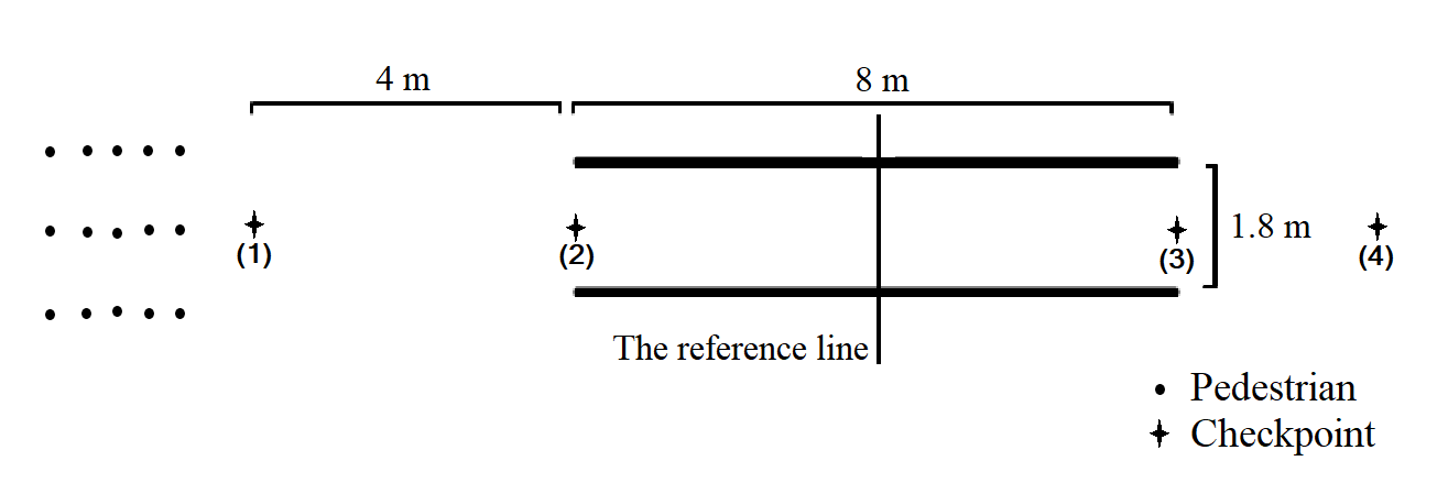
Let us start with and . Following [15], we set for the moment. We take a group of people and simulate their passage through the corridor. The reason why we choose a small crowd is because in a large group of pedestrians the interaction forces become dominant and it is hard to understand the role of other model parameters. The simulation is run for = s, which is the time it takes all the pedestrians to exit the corridor. We take all the combinations of values for and reported in Table 1. We consider a simulation unstable if the speed of one pedestrian exceeds their desired speed or overlaps (of people) and oscillations (of trajectories) occur. From Table 1, we see that if either of the radii is small, i.e. 1 m, the system is unstable. Among the stable combinations, from now on we consider m because it the cheapest computationally.
| m | m | m | |
|---|---|---|---|
| m | unstable | unstable | unstable |
| m | unstable | stable | stable |
| m | unstable | stable | stable |
Next, let us consider the interaction constants in repulsive forces in (6) and in (11). For simplicity, we consider . We note that large values of help avoid overlaps between pedestrians and . On the other hand, when is large and is small, a large value of may give rise to a strong repulsive force that compels a pedestrian to deviate more than 90 degrees away from the target direction, leading oscillations in their trajectory. Our goal is to find a value for that is large enough to avoid overlaps and small enough to avoid oscillations. For this purpose, we increase the number of pedestrians to . For different values of 0, 0.1, 0.2, 0.3, 0.4, 0.5, 0.6, we run simulations and compute overlap and oscillation quantities defined below.
Following [15], we define
| (14) |
where quantifies the “overlap-strength”and is the cardinality of the set . and are the areas of the discs of pedestrians and , and is their area of intersection. If , i.e. no overlap occurs, then is set to . Notice that the maximum value of is 1.
The oscillation-proportion of a simulation is defined as
| (15) |
where is the cardinality of the set . can be viewed as “oscillation-strength” of pedestrian . If , i.e. no oscillation occurs, then is set to Similarly to , the maximum value for is 1.
Fig. 2 shows the average values of and for simulations against . We note that for most of the simulation are unstable (the speed of some pedestrians exceeded their desired speed). We report the results anyways, although they have little significance. From Fig. 2, we see that decreases as , as expected. Aside from the critical values , increases as increases, as expected. The ideal choice appears to be 0.3, which yields no overlap and no oscillations. However, we consider 0.2 an acceptable choice too. Since pedestrians are modeled as discs with a radius that varies with the pedestrian’s speed, we can assume that a pedestrian does not physically occupy the entire disc. Thus, depending on the test we allow some amount of overlaps in the system.
2.3 Validation Against Experimental Data
We quantitatively validate described in model Sec. 2, with the parameters set as explained in Sec. 2.2, by comparing with empirical data from [54]. The experiment geometry is the same as in Fig. 1. A perpendicular line passing through the corridor midline is taken as a reference line. Every pedestrian is assigned the same path: checkpoints 1 to 4. Checkpoint 2 and 4 each have a radius of m (width of the corridor), denoted by . Checkpoint 1 has radius and checkpoint 3 has radius . pedestrians are placed at a distance of m from the corridor entrance. The values of , , and varies for the different experiments. See Table 2.
| Experiment Index | |||
|---|---|---|---|
| 1 | 60 | 0.50 | 1.80 |
| 2 | 66 | 0.60 | 1.80 |
| 3 | 111 | 0.70 | 1.80 |
| 4 | 121 | 1.00 | 1.80 |
| 5 | 175 | 1.45 | 1.80 |
| 6 | 220 | 1.80 | 1.80 |
| 7 | 170 | 1.80 | 1.20 |
| 8 | 160 | 1.80 | 0.95 |
| 9 | 148 | 1.80 | 0.70 |
Over a time interval of length s, the macroscopic quantities flux , average velocity and density are calculated as follows:
| (16) |
where is the total number of people who crossed the reference line during , is the time taken by these pedestrians to cross the reference line, and is the velocity of the pedestrian at the time they cross the reference line. For every experiment, we will compare the computed and measured quantities defined in (16).
Let , . To decide which to pick, we consider experiment 1 in Table 2. Fig. 3 shows the computed average velocity plotted against density for different . We see that when is in s, the density values are close to each other. Thus, we set s for experiment 1. The values of for all the other experiments in Table 2 are set in a similar manner. Then, the densities and average velocities are averaged over runs per experiment.
Fig. 4 shows the computed and measured (from [54]) fundamental diagram for each experiment in Table 2. We observe good agreement: the overall trend is similar, although for certain experiments the computed average velocity for a given density is slightly smaller than the corresponding measured quantity. We remark that the parameters in our model were set as explained in Sec. 2.2 and not tuned to fit the measured data. Thus, some slight difference is to be expected.
3 Bidirectional flow
The experimental validation of our model in Sec. 2.3 involves unidirectional flow of pedestrians. In this section, we consider bidirectional flow. It is know that when groups of people approach each other from opposite directions, they form lanes (see, e.g., [22, 21, 53]), which increase the flow efficiency. We aim at checking that our model, calibrated as reported in Sec. 2.2, can reproduce this spontaneous crowd behavior.
We consider a m long and m wide corridor. Two groups of equal size are initially placed at opposite corridor ends, moving towards each other. Since lane emergence is not immediate, we simulate a periodic corridor. We vary the pedestrian density inside the corridor from to pedestrians/m2, with increment pedestrians/m2. Higher values of were not considered as they led to an unstable system in such a small geometry. Recall that for unidirectional flow we could simulate up to pedestrians/m2 without instabilities (see Fig. 4). So, bidirectional flow in a confined environment seems to be challenging for our model. The number of pedestrians for each experiment is calculated by , where with m2 is the corridor area. For all the simulation, every pedestrian has a desired speed of 1 m/s. We remark that pedestrians cannot be initially placed in a symmetric configuration in order to avoid a “frozen state”. See Fig. 5. We let each simulation run until the lane configuration remains stable for minute.

Table. 3 reports the number of lanes formed in each experiments. We observe that for two lanes form, while for four lanes form. Fig. 6 show the lane configuration for = and . In Fig. 6 (b) we see that the row of pedestrians near the wall tend to get closer to the wall when they encounter the opposing stream of pedestrians.This is due to the fact that the repulsive force from pedestrians (6) is higher than the repulsive force from the walls (11). When we considered , we observed two lanes before the system became unstable. See Fig. 7. Notice that we used a different initial configuration than in the case in the effort to obtain a stable system. This suggests that the number of lanes for a short period of time is influenced not only by the crowd size but also by the initial positioning.
| Density | 0.2 | 0.4 | 0.6 | 0.8 | 1.0 | 1.2 | 1.4 | 1.6 |
|---|---|---|---|---|---|---|---|---|
| Number of pedestrians | 20 | 40 | 60 | 80 | 100 | 120 | 140 | 160 |
| Number of lanes | 2 | 2 | 2 | 2 | 2 | 2 | 4 | 4 |


4 Simulation of airborne disease spreading using pedestrian dynamics
With the goal of studying the onset of an airborne disease spreading in a complex, yet confined environment we extend the model presented in Sec. 2 by introducing a simple method to trace contact. Depending on the nature of the disease, the sufficient contact time to infect a susceptible person varies. We will focus on a highly infectious disease, like measles.
4.1 A simple model for the spreading of a highly infectious disease
Let us consider a group of pedestrians in a geometry . Pedestrians can be: sick (infectious), immune (non-susceptible), vulnerable (susceptible), infected and not infected. We define the set of the susceptible and infectious people:
respectively. In each simulation, of the population is immune and only a small number of people are sick. The rest of the population is vulnerable.
For a sick person with position , we define the set of all susceptible pedestrians that lie inside its circle of influence (sickness domain) at a certain time as:
where denotes the Euclidean norm in and is the cutoff radius for the circle of influence. If a pedestrian stays in for a continuous period of time, e.g. minutes, then they have a probability of getting infected. After minutes, pedestrian is moved to either one of the following sets according to its updated stage:
Once a vulnerable pedestrian moves to either of these sets, they are no longer considered to be in the population that could get infected by sick people, i.e.,
We also assume that pedestrians belonging to are not able to transmit the disease, although infected. At the end of each simulation, we will have the number of secondary contacts for the simulated scenario.
In order to simulate the disease spreading in airport terminals, we implemented the pedestrian dynamics model in Sec. 2 and the above contact tracing method in C++. All the simulations ran on a shared 40-core computing server with 512 GB RAM.
4.2 Numerical Results
We consider terminals in two US airports, Hobby Airport in Houston and the Atlanta International Airport, as concrete settings to test our pedestrian dynamics model with contact tracing. We will examine different scenarios: variable population size, variable percentage of immune (non-susceptible) population, boarding bridges or boarding buses. Through the numerical simulations, we quantify the increase in average number of secondary contacts increases as a given terminal becomes more densely populated, the percentage of immune people decreases, the number of primary contacts increases, and areas of high density (such as the boarding buses) are present.
Since we deal with more complicated geometries that the ones tested in Sec. 2 and 3, we handle the checkpoint assignment in a different way. The list of checkpoints contains, for a given checkpoint , the checkpoint position and a radius . If checkpoint is in a person’s path, the position of the checkpoint for that particular person is randomly picked to be a point inside the circle of radius centered at checkpoint ’s position. This makes each pedestrian’s checkpoints unique (if truly random). In addition, this way to assign checkpoints helps to avoid oscillations in pedestrian motion due to clustering of pedestrians around checkpoints that have wait times.
4.3 Hobby Airport in Houston
We consider a part of Houston’s William P. Hobby (HOU) Airport as a sample geometry . See Fig. 8. At the start, each of the pedestrian in is randomly categorized to be either sick, immune or vulnerable. Pedestrians are assigned a random path to pass through the airport. Some people deplane, enter the airport through the terminal gate and leave the airport via the exit corridor. Others enter the airport through the entry corridor and walk to their assigned terminal gate. Random people are selected to use the restrooms or stop at a restaurant. Departing people are also assigned to randomly check display monitors. Appropriate wait times are allocated for each checkpoint that denotes a restroom, restaurant or a display monitor. Finally, if a person reaches the gate before their boarding time, they stay in the wait area near their assigned gate until it is time to board.

The pedestrian dynamics model parameters are set as follows: s, s, s, m, m, and . For the contact tracing, we set m and . The latter is a realistic value for a highly infectious disease. will vary from to with . Remark that herd immunity for a highly infectious disease, like measles, is over 90%. For each , 200 simulations are run to calculate the average number of secondary contacts, which is denoted by .
We will consider a simple case to test our implementation (case 1) and a more realistic case (case 2):
- -
Case 1: = 400, = minutes, = 1 minute.
- -
Case 2: = 1000, = minutes, = minutes.
For each case, we consider two scenarios: a) 1 primary contact and b) 2 primary contacts. We remark that both cases feature a low pedestrian density, given the size of the domain. As expected, our model can handle them efficiently.
Fig. 9 shows two snapshots of a simulation for case 1b. Dots denote people and the color refers to their characterization: red for sick (primary contact), green for immune, black for vulnerable, cyan for infected (secondary contact), and orange for not infected. In Fig. 9 (top), people are deplaning from the rightmost gate while people at the leftmost gate are waiting to deplane. In Fig. 9 (bottom), we see that the primary contact infected several surrounding people in the waiting area.


Fig. 10 shows the average number of secondary contacts for varying . We note that with the exception of = for case 1, when decreases the number of secondary contacts increases for both cases. We also note that for case 1 increases slowly as decreases, while the rate of increase of is faster for case 2.
Table 4 reports the computed average number of secondary contacts , standard deviation for all 200 simulations and maximum number of secondary contacts among all the simulations for cases 1a and 2b, respectively. We see that as decreases, the standard deviation of the number of secondary contacts increases, indicating a wider range of values for the number of secondary contacts. This is reinforced by Fig. 11, where we compare the frequency distributions for cases 1a and 2b. The curves for larger values have taller, narrower peaks as opposed to the curves for smaller values. From Fig. 11 (a) we see that the mode of every distribution is zero, while the mode of every distribution in Fig. 11 (b) is different from zero.
| Case 1a | ||||||||
| 90 | 85 | 80 | 75 | 70 | 65 | 60 | 55 | |
| 0.56 | 0.66 | 0.88 | 0.69 | 0.83 | 0.94 | 1.15 | 1.44 | |
| 0.93 | 0.85 | 0.99 | 1.19 | 1.19 | 1.12 | 1.31 | 1.53 | |
| 4 | 4 | 4 | 7 | 7 | 6 | 7 | 9 | |
| Case 2b | ||||||||
| 90 | 85 | 80 | 75 | 70 | 65 | 60 | 55 | |
| 1.37 | 2.10 | 2.75 | 3.47 | 4.37 | 5.05 | 5.64 | 5.94 | |
| 1.30 | 1.66 | 2.04 | 2.53 | 2.69 | 2.80 | 3.37 | 3.57 | |
| 6 | 7 | 10 | 17 | 15 | 15 | 16 | 16 | |
Although at HOU airport passengers board through a boarding bridge, we extend the geometry in Fig. 8 to include buses to transport passengers from the gate to the plane. This is to compare the disease spreading in an airport with and without buses. Every departing pedestrian will have their final checkpoint as a random position inside a bus. The pedestrians stay in the bus for 5 minutes and then they board the plane. A bus is 5 m x 12 m and can accommodate 50 people. Fig. 12 shows a screenshot of a simulation in HOU Airport with buses.

We run 200 simulations, with the parameters set as in the case of no buses, in order to calculate for = , , , . Fig. 13 shows produced in HOU Airport with and without buses. The data in Fig. 13 (a) is the same as in Fig. 10, but with a different scale to facilitate the comparison with Fig. 13 (b). We see that having a high density area such as a bus in the path of pedestrians drastically increases the rate at which people get infected, for a given value of . In addition, the rate at which increases as decreases is faster in the airport with buses. We report in Fig. 14 the average number of secondary contacts generated inside the bus. We observe that the cases with the same number of primary contacts have average values closer to each other. The population size makes less of a difference because the number of people in the buses does not change significantly between case 1 and 2.
Finally, to estimate the basic reproduction number, we set for cases 1a and 2a. Table 5 reports the basic reproduction number averaged over 200 simulations for both cases without and with buses. For both cases, the buses contribute to an increase of roughly 5 infected people.
| Without Buses | With Buses | |
|---|---|---|
| case 1a | 2.4 | 7.66 |
| case 2a | 9.305 | 15.21 |
4.4 Connecting airports: Hobby Airport to Atlanta International Airport
The set of tests presented in this section involves one or two primary contacts that takes a flight from Hobby Airport (shown in Fig. 8) to Hartsfield-Jackson Atlanta International (ATL) Airport. We will only consider the part of ATL airport shown in Fig. 15. In all the simulations, the primary contact(s) enters HOU airport through security check, moves through the terminal to reach the gate of their flight, boards the plane to ATL airport. Once at ATL airport, the primary contact(s) moves through the terminal to reach the gate of their final flight. Just like for the results in Sec. 4.3, some people enter ATL airport through the entry corridor and board a flight, while others enter through the gates. Ten percent of the latter group goes onto boarding a flight, while the rest leave the airport through the exit. In addition, random people are selected to use the restrooms or stop at a restaurant and departing people are also assigned to randomly check display monitors. We will consider the case of both airports with and without buses.

All the parameters are set like in Sec. 4.3. However, we limit the values of to , , , and we consider only one case: = 1000, = minutes, = minutes, with a) 1 primary contact and b) 2 primary contacts. For each scenario, we run 200 simulations and calculate the average number of secondary contacts .
To simplify the simulation, the sick person can infect vulnerable people only inside the terminals and, if present, in the buses. In this way, the simulations in each airport can be run in parallel. Fig. 16 (a) shows the initial people distribution for one of the simulations in ATL airport with the buses. The pedestrians inside the buses spend 5 minutes there before they reach the terminal. The people in the terminal are waiting to board their planes. The rest of the pedestrians, including the primary contact(s), will enter the airport later as per their assigned arrival time (if deplaning) or minutes into the simulation (if entering through the entry corridor). Fig. 16 (b) shows the people distribution and characterization after 20 minutes.


Fig. 17 reports the the average number of secondary contacts for case 1a and 1b with and without buses. By comparing Fig. 17 (a) and (b), we see that the number of secondary contacts is more than doubled in presence of the buses. These results confirm that: (i) a high percentage of immune pedestrians in the system ensures that the number of infected people remain small and (ii) the spreading of the disease is amplified by the airport buses.
Fig. 18 displays the average number of secondary contacts produced inside the buses vs inside the ATL terminal for cases 1a and 1b. We notice that the average number of people infected by one primary contact inside the buses is close to the average number of people infected by two primary contacts inside the terminal.
Finally, to estimate the basic reproduction number in ATL airport we set for case 1a. Table 6 reports the basic reproduction number averaged over 200 simulations for cases 1a without and with buses.
| Without Buses | With Buses | |
| Case 1a | 7.263 | 18.693 |
5 Conclusions
We combined a grid free, force-based microscopic model for pedestrian dynamics with a contact tracing method to study the initial spreading of a highly infectious airborne disease in a confined environment. The pedestrian dynamics model is calibrated to avoid unrealistic pedestrian motion (overlap of people and oscillating walking trajectories) and validated against empirical data from [54]. In addition, we showed that lane formation in bidirectional flow (a well known self organizing phenomenon) is captured by the pedestrian dynamics model under consideration. The contact tracing method uses a sickness domain around each sick person. A susceptible person has a prescribed probability to become infected if they stay in a sickness domain for a certain amount of time.
To test our model of pedestrian dynamics with contact tracing, we considered medium size populations with immune and susceptible people in the terminals of two US airports. We computed the average number of secondary contacts produced by one or two primary contacts in a single terminal or in terminals of different airports connected by a flight hosting a primary contact. We also considered the case where people could board a bus to reach their planes. Sick people were traced only when inside airports or buses. In the case of airports without buses, we concluded that:
- -
For same size populations, an increase in primary contacts causes an increase in the average number of infected pedestrians that becomes larger as the percentage of immune population decreases.
- -
The larger the population size, the higher the rate of increase in the average number of infected pedestrians.
- -
A higher population density leads to an increase in average number of secondary contacts for a fix percentage of immune population.
In the case of airports with buses (high density areas), we showed the drastic increase in the rate at which people are getting infected.
The combination of pedestrian dynamics model with contact tracing method could be used in different settings (emergency rooms, hospitals, etc.) and tailored to airborne diseases with different spreading mechanisms. If further tested and validated, it could become a tool to investigate best practices that can help reduce the spreading of a disease.
Acknowledgements
This work has been partially supported by NSF through grant DMS-1620384. We acknowledge fruitful discussions with Drs. Ilya Timofeyev and William Fitzgibbon.
References
- [1] J. P. Agnelli, F. Colasuonno, and D. Knopoff. A kinetic theory approach to the dynamics of crowd evacuation from bounded domains. Mathematical Models and Methods in Applied Sciences, 25(01):109–129, 2015.
- [2] Frank G. Ball, Edward S. Knock, and Philip D. O’Neill. Threshold behaviour of emerging epidemics featuring contact tracing. Advances in Applied Probability, 43(4):1048–1065, 2011.
- [3] N. Bellomo, D. Knopoff, and J. Soler. On the difficult interplay between life, “complexity”;, and mathematical sciences. Mathematical Models and Methods in Applied Sciences, 23(10):1861–1913, 2013.
- [4] N. Bellomo, B. Piccoli, and A. Tosin. Modeling crowd dynamics from a complex system viewpoint. Mathematical Models and Methods in Applied Sciences, 22(supp02):1230004, 2012.
- [5] Nicola Bellomo and Abdelghani Bellouquid. On the modeling of crowd dynamics: Looking at the beautiful shapes of swarms. Networks and Heterogeneous Media, 6(3):383–399, 2011.
- [6] Nicola Bellomo, Abdelghani Bellouquid, Livio Gibelli, and Nisrine Outada. A quest towards a mathematical theory of living systems. Modeling and Simulation in Science, Engineering and Technology. Birkhauser, 2017.
- [7] Nicola Bellomo, Abdelghani Bellouquid, and Damian Knopoff. From the microscale to collective crowd dynamics. SIAM Multiscale Model. Simul., 11:943–963, 2013.
- [8] Nicola Bellomo and Christian Dogbe. On the modeling of traffic and crowds: A survey of models, speculations, and perspectives. SIAM Review, 53(3):409–463, 2011.
- [9] Nicola Bellomo and Livio Gibelli. Toward a mathematical theory of behavioral-social dynamics for pedestrian crowds. Math. Models Methods Appl. Sci., 25(13):2417–2437, 2015.
- [10] Nicola Bellomo and Livio Gibelli. Behavioral crowds: Modeling and Monte Carlo simulations toward validation. Computers and Fluids, 141:13–21, 2016.
- [11] Nicola Bellomo, Livio Gibelli, and Nisrine Outada. On the interplay between behavioral dynamics and social interactions in human crowds. Kinetic and Related Models, 12(2):397–409, 2019.
- [12] Glenn Webb Cameron Browne, Hayriye Gulbudak. Modeling contact tracing in outbreaks with application to ebola. Journal of Theoretical Biology, 384:33–49, 2015.
- [13] M. Chraibi, A. Seyfried, A. Schadschneider, and W. Mackens. Quantitative description of pedestrian dynamics with a force-based model. In IEEE/WIC/ACM International Joint Conference on Web Intelligence and Intelligent Agent Technology IEEE Computer Society, Los Alamitos, CA, volume 3, pages 583–586, 2009.
- [14] Mohcine Chraibi, Ulrich Kemloh, Andreas Schadschneider, and Armin Seyfried. Force-based models of pedestrian dynamics. Networks and Heterogeneous Media, 6(3):425–442, 2011.
- [15] Mohcine Chraibi, Armin Seyfried, and Andreas Schadschneider. Generalized centrifugal-force model for pedestrian dynamics. Phys. Rev. E, 82:046111, Oct 2010.
- [16] Martin Eichner. Case isolation and contact tracing can prevent the spread of smallpox. American Journal of Epidemiology, 158:118–128, 2003.
- [17] C Fraser, S Riley, R.M Anderson, and Ferguson N.M. Factors that make an infectious disease outbreak controllable. Proc. Natl Acad. Sci. USA, 101:6146–6151, 2004.
- [18] Anderson R.M Garnett G.P. Sexually transmitted diseases and sexual behavior: insights from mathematical models. J. Infect. Dis., 174:S150–S161, 1996.
- [19] Giorgio Guzzetta, Marco Ajelli, Zhenhua Yang, Leonard N. Mukasa, Naveen Patil, DeniseE. Kirschner, and Stefano Merler. Effectiveness of contact investigations for tuberculosis control in Arkansas. Journal of Theoretical Biology, 380:238–246, 2015.
- [20] Dirk Helbing. A mathematical model for the behavior of pedestrians. Behavioral Science, 36(4):298–310, 1991.
- [21] Dirk Helbing. Collective phenomena and states in traffic and self-driven many-particle systems. Computational Materials Science, 30(1�2):180 – 187, 2004. Selected papers of the Twelfth International Workshop on Computational Materials Science (CMS2002).
- [22] Dirk Helbing and Péter Molnár. Social force model for pedestrian dynamics. Phys. Rev. E, 51:4282–4286, May 1995.
- [23] Dirk Helbing and Tamas Vicsek. Optimal self-organization. New Journal of Physics, 1(1):13, 1999.
- [24] Yorke J.A Hethcote H.W. Gonorrhea transmission dynamics and control. Springer Lecture Notes in Biomathematics, Berlin:Springer, 1984.
- [25] Roger L. Hughes. A continuum theory for the flow of pedestrians. Transportation Research Part B: Methodological, 36(6):507 – 535, 2002.
- [26] James M. Hyman, Jia Li, and E. Ann, Stanley. Modeling the impact of random screening and contact tracing in reducing the spread of HIV. Mathematical Biosciences, 181:17–54, 2003.
- [27] Anders Johansson, Dirk Helbing, and Pradyumn K. Shukla. Specification of the social force pedestrian model by evolutionary adjustment to video tracking data. Advances in Complex Systems, 10(supp02):271–288, 2007.
- [28] McKendrick A.G Kermack W.O. A contribution to the mathematical theory of epidemics. Proc. R. Soc., 115:700–721, 1927.
- [29] Daewa Kim and Annalisa Quaini. A kinetic theory approach to model pedestrian dynamics in bounded domains with obstacles. Kinetic and Related Models, 12(6):1273–1296, 2019.
- [30] Istvan Z Kiss, Darren M Green, and Rowland R Kao. Disease contact tracing in random and clustered networks. Proceedings of the Royal Society B, 272:1407–1414, 2005.
- [31] Don Klinkenberg, Christophe Fraser, and Hans Heesterbeek. The effectiveness of contact tracing in emerging epidemics. PLOS ONE, 1(1):1–7, 12 2006.
- [32] Taras I. Lakoba, D. J. Kaup, and Neal M. Finkelstein. Modifications of the Helbing-Molnar-Farkas-Vicsek social force model for pedestrian evolution. SIMULATION, 81(5):339–352, 2005.
- [33] S. Liu, S. Lo, J. Ma, and W. Wang. An agent-based microscopic pedestrian flow simulation model for pedestrian traffic problems. IEEE Transactions on Intelligent Transportation Systems, 15(3):992–1001, June 2014.
- [34] Shaobo Liu, Lizhong Yang, Tingyong Fang, and Jian Li. Evacuation from a classroom considering the occupant density around exits. Physica A: Statistical Mechanics and its Applications, 388(9):1921 – 1928, 2009.
- [35] Jian Ma, Wei guo Song, Jun Zhang, Siu ming Lo, and Guang xuan Liao. k-nearest-neighbor interaction induced self-organized pedestrian counter flow. Physica A: Statistical Mechanics and its Applications, 389(10):2101 – 2117, 2010.
- [36]
MATLAB.
https://www.mathworks.com/products/matlab.htm. - [37]
Notes from the Field: Measles Transmission at a Domestic Terminal Gate in an
International Airport – United States, January 2014.
https://www.cdc.gov/mmwr/preview/mmwrhtml/mm6350a9.htm. - [38]
Notes from the Field: Measles Transmission in an International Airport at a
Domestic Terminal Gate – April-May 2014.
https://www.cdc.gov/mmwr/preview/mmwrhtml/mm6424a6.htm. - [39] Mehdi Moussaïd, Dirk Helbing, Simon Garnier, Anders Johansson, Maud Combe, and Guy Theraulaz. Experimental study of the behavioural mechanisms underlying self-organization in human crowds. Proceedings of the Royal Society of London B: Biological Sciences, 276(1668):2755–2762, 2009.
- [40] Anuj Mubayi, Christopher Kribs Zaleta, Maia Martcheva, and Carlos Castillo-Chavez. A cost-based comparison of quarantine strategies for new emerging diseases. Mathematical Biosciences and Engineering, 7(1551-0018-2010-3-687):687, 2010.
- [41] Johannes Mueller, Mirjam Kretzschmar, and Klaus Dietz. Contact tracing in stochastic and deterministic epidemic models. Mathematical Biosciences, 164:39–64, 2000.
- [42] D.R. Parisi and C.O. Dorso. Morphological and dynamical aspects of the room evacuation process. Physica A: Statistical Mechanics and its Applications, 385(1):343 – 355, 2007.
- [43] K. Rathinakumar. A Microscopic Approach to Pedestrian Dynamics and the Onset of Disease Spreading. PhD thesis, University of Houston, 2019.
- [44] C.M. Rivers, E.T. Lofgren, M. Marathe, S. Eubank, and B.L. Lewis. Modeling the impact of interventions on an epidemic of ebola in Sierra Leone and Liberia. PLoS Curr.,6, 2014.
- [45] P Rohani, D.J.D Earn, and B.T Grenfell. The impact of immunisation on pertussis transmission in england and wales. Lancet, 355:285–286, 2000.
- [46] Andreas Schadschneider, Wolfram Klingsch, Hubert Klüpfel, Tobias Kretz, Christian Rogsch, and Armin Seyfried. Evacuation Dynamics: Empirical Results, Modeling and Applications, pages 517–550. Springer New York, New York, NY, 2011.
- [47] Armin Seyfried, Oliver Passon, Bernhard Steffen, Maik Boltes, Tobias Rupprecht, and Wolfram Klingsch. New insights into pedestrian flow through bottlenecks. Transportation Science, 43(3):395–406, 2009.
- [48] A. Shende, M. P. Singh, and P. Kachroo. Optimization-based feedback control for pedestrian evacuation from an exit corridor. IEEE Transactions on Intelligent Transportation Systems, 12(4):1167–1176, Dec 2011.
- [49] Yusuke Tajima, Kouhei Takimoto, and Takashi Nagatani. Pattern formation and jamming transition in pedestrian counter flow. Physica A: Statistical Mechanics and its Applications, 313(3):709 – 723, 2002.
- [50] Alasdair Turner and Alan Penn. Encoding natural movement as an agent-based system: An investigation into human pedestrian behaviour in the built environment. Environment and Planning B: Planning and Design, 29(4):473–490, 2002.
- [51] Jonathan A. Ward, Andrew J. Evans, and Nicolas S. Malleson. Dynamic calibration of agent-based models using data assimilation. Royal Society Open Science, 3(4), 2016.
- [52] S. Xu and H. B. L. Duh. A simulation of bonding effects and their impacts on pedestrian dynamics. IEEE Transactions on Intelligent Transportation Systems, 11(1):153–161, March 2010.
- [53] W. J. Yu, R. Chen, L. Y. Dong, and S. Q. Dai. Centrifugal force model for pedestrian dynamics. Phys. Rev. E, 72:026112, Aug 2005.
- [54] J. Zhang, W. Klingsch, A. Schadschneider, and A. Seyfried. Transitions in pedestrian fundamental diagrams of straight corridors and T-junctions. J. Stat. Mech., 2011:P06004, 2011.
- [55] B. Zhou, X. Wang, and X. Tang. Understanding collective crowd behaviors: Learning a mixture model of dynamic pedestrian-agents. In 2012 IEEE Conference on Computer Vision and Pattern Recognition, pages 2871–2878, June 2012.