Simple formulas of directional amplification from non-Bloch band theory
Abstract
Green’s functions are fundamental quantities that determine the linear responses of physical systems. The recent developments of non-Hermitian systems, therefore, call for Green’s function formulas of non-Hermitian bands. This task is complicated by the high sensitivity of energy spectrums to boundary conditions, which invalidates the straightforward generalization of Hermitian formulas. Here, based on the non-Bloch band theory, we obtain simple Green’s function formulas of general one-dimensional non-Hermitian bands. Furthermore, in the large-size limit, these formulas dramatically reduce to finding the roots of a simple algebraic equation. As an application, our formulation provides the desirable formulas for the defining quantities, the gain and directionality, of directional amplification. Thus, our formulas provide an efficient guide for designing directional amplifiers.
The responses of a physical system are generally proportional to a small external perturbation, which is captured by the Green’s functions. Whereas their explicit formulas are well known for Hermitian energy bands, recent progresses in non-Hermitian systems call for their generalizations. This seemingly straightforward task is hindered by the non-Hermitian skin effectYao and Wang 2018; Kunst et al. 2018; Lee and Thomale 2019; Martinez Alvarez et al. 2018; Xiao et al. 2020; Helbig et al. 2020; Ghatak et al. 2020, meaning the exponential localization of most eigenstates to the boundaries. This effect causes a high sensitivity of Green’s functions to the boundary condition, invalidating a straightforward extension of Hermitian formulas. It is the purpose of this paper to obtain general formulas of non-Hermitian Green’s functions.
The problem can be simply phrased. Let us consider a general non-Hermitian Hamiltonian of one-dimensional (1D) lattice with length , with translational symmetry (for ). For example, if we take and all other matrix elements zero, can be shown pictorially as Fig. 1(a). We take open-boundary condition (OBC) at the two ends11 1 Our results will be generalizable to other boundary conditions such as domain wall systems. In mathematical literature, OBC corresponds to Toeplitz matrices, while PBC corresponds to circulant matrices. . Our goal is to find explicit formulas for the frequency-domain Green’s function matrix
| (1) |
Although Green’s functions have recently been studied to extract non-Hermitian topologyBorgnia et al. 2020; Zirnstein et al. 2019; Silveirinha 2019, their general and explicit formulas have been lacking. As we will see, this seemingly trivial goal is difficult, if not impossible, to achieve from the standard Brillouin zone (BZ) and Bloch-band framework. Here, we will obtain the matrix from the non-Bloch band theoryYao and Wang 2018; Yokomizo and Murakami 2019, which is based on the generalized Brillouin zone (GBZ) originally introduced to understand non-Hermitian topologyYao and Wang 2018; Yao et al. 2018; Yokomizo and Murakami 2019; Lee and Thomale 2019; Longhi 2019; Yang et al. 2020; Deng and Yi 2019; Longhi 2020; Kawabata et al. 2020; Liu et al. 2019; Song et al. 2019a; Lee et al. 2020; Yi and Yang 2020; Bergholtz et al. 2021; Ashida et al. 2020. We obtain a simple integral formula for all the matrix elements . In particular, for the end-to-end Green’s functions, and , our integral formula reduces in the large- limit to:
| (2) |
where are the roots of ordered as . Here, denotes the Bloch Hamiltonian of , under the notation , which takes the general form of with coefficients , being the hopping range. For example, for the model Fig. 1(a), we have and
| (3) |
As we will show, the presence in Eq. (2) of the middle two roots, namely the -th and -th of the roots, reflects the GBZ origin of Eq. (2).
Among various applications, our formulas are important for directional amplifiers (or nonreciprocal amplifiers). In such devices, signals are amplified in a preferred direction and suppressed in the reversed direction, which protects the signal sources; such feature is essential to a wide range of applications in classical and quantum information processingAbdo et al. 2013; Abdo et al. 2014; Sliwa et al. 2015; Jalas et al. 2013; Feng et al. 2011; Caloz et al. 2018; Fleury et al. 2014; Sounas and Alù 2017; Yu and Fan 2009; Estep et al. 2014; Soljačić et al. 2003; Metelmann and Clerk 2015; Ranzani and Aumentado 2015; Fang et al. 2017; Barzanjeh et al. 2017; Peterson et al. 2017; Bernier et al. 2017; Xu et al. 2019. Irrespective of device details, their dynamics is generated by effective non-Hermitian HamiltoniansMetelmann and Clerk 2015; Ranzani and Aumentado 2015; Porras and Fernández-Lorenzo 2019; Peterson et al. 2017; Bernier et al. 2017; Fang et al. 2017; Barzanjeh et al. 2017; Xu et al. 2019; Ruesink et al. 2016; Barzanjeh et al. 2018; McDonald et al. 2018; Wanjura et al. 2020; Wang et al. 2019; Malz et al. 2018; Mercier de Lépinay et al. 2019, and the gain and directionality are given by the Green’s functionMetelmann and Clerk 2015; Ranzani and Aumentado 2015; Porras and Fernández-Lorenzo 2019. To be precise, directional amplification occurs when while for a certain pair , meaning that a -frequency signal is amplified from to , while the back-propagation from to is suppressed. Although brute force calculation of Green’s function is viable for few-mode cases, it becomes inconvenient for many-mode amplifiers taking the shape of a 1D chain; such 1D amplifiers have the advantage of unlimited gain-bandwidth product without fine tuningMcDonald et al. 2018; Wanjura et al. 2020. Our Green’s function formulas tell their gain and directionality in a simple fashion.


Integral formulas of Green’s function.–Numerically, follows an exponential law with respect to . For example, the end-to-end Green’s functions for our specific model [Fig. 1(a)] have the following large- behaviors,
| (4) |
which is displayed in Fig. 1(b). Knowing and is important to understanding and designing directional amplification. The condition for rightward amplification, and , is to require and ; similarly, the condition for leftward amplification is to require . Remarkably, such 1D amplification does not suffer from the standard limitation of gain-bandwidth product, because large gain is possible for large , while the bandwidth is independent of McDonald et al. 2018; Wanjura et al. 2020.
The values of and can be derived from the general formulas of to be obtained below. To derive the general , a plausible starting point is the spectral representation , where and are the eigenvalues and normalized right (left) eigenvectors of under OBC, namely, . Moreover, it is tempting to switch to the BZ and conjecture that
| (5) |
With the notation , BZ is the unit circle and the integral becomes:
| (6) |
An immediate difficulty is seen after using the residue theorem, which leads to , being the largest-modulus root of inside the unit circle. This would always imply and forbids any directional amplification. Similarly, one would have , being the smallest-modulus root outside the unit circle. In fact, Eq. (6) is generally valid only in Hermitian cases, as will become clear below.
The problem with Eq. (6) is the assumption of the validity of Bloch band theory. In fact, a unique non-Hermitian phenomenon is that, for a broad class of non-Hermitian Hamiltonians, all the eigenstates are localized at the boundaries, which is known as the non-Hermitian skin effectYao and Wang 2018; Kunst et al. 2018; Lee and Thomale 2019; Martinez Alvarez et al. 2018; Xiao et al. 2020; Helbig et al. 2020; Ghatak et al. 2020. This effect suggests that we should remove the usual Bloch-band restriction . Indeed, it has been found that when varies in a closed curve known as the GBZ in the complex plane, the trajectory of is exactly the OBC energy bandYao and Wang 2018; Yokomizo and Murakami 2019. Note that if varies in the BZ (), the trajectory is the periodic-boundary-condition (PBC) energy band, which is generally different from the OBC energy band. In Hermitian cases, GBZ reduces to the BZ, being consistent with the fact that PBC and OBC bands are the same. The equation that determines the GBZ was found in Refs. Yao and Wang 2018; Yokomizo and Murakami 2019; we recall their final result below without reproducing the technical derivations. For a hopping range , is a -th order equation with roots , which are ordered as . The GBZ equation readsYao and Wang 2018; Yokomizo and Murakami 2019
| (7) |
which is essentially a single-variable equation because , , are related by . The and solutions form a closed loop in the complex plane, which is the GBZ, and the solutions form the OBC energy bands. Examples of GBZ are shown in Fig. 2(a)(e).
In view of the failure of BZ [e.g. invalidity of Eq. (6)], we propose the following GBZ-based integral formula for :
| (8) |
which is a main result of this paper. Its proof is provided in Supplemental Material. In practice, this integral is highly convenient to evaluate by the residue theorem, which reduces it to a sum at several roots of . This simplification is enabled by the vital fact that the GBZ is always a closed loopYao and Wang 2018; Yokomizo and Murakami 2019; Yang et al. 2020. A numerical confirmation of Eq. (16) is shown in Fig. 1(c). Irrespective of being large or small, the formula is always precise for not too close to the two ends. At the two ends, because of the boundary effect, a factor of order unity has to be included:
| (9) | |||||
| (10) |
Now Eq. (2) can be derived as follows. Ordering the roots of as , one can prove that are enclosed by the GBZ, while are not. To see this, suppose that we vary in the complex plane (though is real-valued for physical applications). As long as stays away from the OBC energy spectrum , the roots ’s cannot touch the GBZ because GBZ generates . Therefore, the number of roots enclosed by GBZ is independent of . To determine this number, we consider the limit, in which either the or term dominates and there are roots with , and also roots with . Therefore, for any , there are roots inside the GBZ (For a more rigorous proof, see Refs.Zhang et al. 2020; Okuma et al. 2020). Now Eq. (9) and Eq. (10) can be simplified by the residue theorem. For large , we obtain Eq. (2), in other words,
| (11) |
Therefore, the middle two roots of , and , determine the gain and directionality, leading to a surprising simplification. The indices and are difficult to understand from the BZ; they reflect the GBZ origin of Eqs. (2)(11). Eqs. (16-11) are the central results of this work. For multi-band systems, is a matrix, and Eq. (11) remains applicable with denoting the roots of sup.
As an application to the model in Fig. 1(a), we show in Fig. 2 a quantitative comparison of our theory with the extensive numerical results. For all the parameters investigated, the numerical and are in excellent agreement with Eq. (11) with . Pictorially, rightward and leftward amplification occurs when a root locates in the colored area in Fig. 2(a) and (e), respectively. Notably, the amplifier can selectively amplify signals in a frequency-dependent direction. In our theory, this frequency-dependent directionality is possible when the GBZ has intersections with the BZ [Fig. 2(a)(e)]. This picture provides a mechanism for designing devices that efficiently integrate directional amplifiers and frequency filters or splitters. On the other hand, the simpler cases of rightward (leftward) unidirectional amplification within the entire bandwidth are realized when the GBZ is entirely outside (inside) the BZ (an example is shown in Supplemental Material).
Intuitively, the nonreciprocal hoppings seem to favor motion towards a preferred direction, causing directional amplification in that direction; e.g. when in Fig. 1(a), it seems that the directional amplification should be rightward. However, as has been shown above, leftward directional amplification is also seen in certain frequency window. Thus, the simple intuition based on hopping direction fails even qualitatively by telling a wrong amplification direction. Our formulas of are therefore not merely a matter of quantitative precision, but also important for a qualitative prediction.
Very recently, effort has been made to find OBC Green’s function formulas from conventional Brillouin zoneWanjura et al. 2020. Their results are applicable only to the simplest case where the hoppings exist only between nearest neighbors, in which case our results are consistent with theirs. It is highly challenging, if not impossible, to generalize their approach to the cases beyond nearest-neighbor hopping [e.g. our model Fig. 1(a)]. In contrast, our formulas are straightforward to use for general hoppings. Note that the necessity of taking OBC has been emphasized in recent insightful papersMcDonald et al. 2018; Wanjura et al. 2020, though general formulas were lacking. In fact, if one takes PBC, the directional amplifiers become dynamically unstable, which results from the endless amplification during the cyclic directional motion.
We note that our results are generalizable to more complicated boundary conditions such as domain wall geometries, for which GBZ remains definableDeng and Yi 2019. Moreover, as the concept of GBZ also applies to higher dimensionsYao et al. 2018; Liu et al. 2019, we expect that higher-dimensional generalizations of our formulas remain valid, though their applications rely on efficient algorithms of GBZ, which are called for in higher dimensions.
Realization in open quantum systems.–So far, the non-Hermitian Hamiltonian is taken for granted. While it is without question in classical platforms, for example, the Green’s function is directly measurable in the topolectrical circuitsHelbig et al. 2020, we emphasize that our formulas are also applicable to various open quantum systems. For example, we may consider a 1D lattice of coupled bosonic modes, which can be realized in various realistic systems such as optomechanical cavitiesAspelmeyer et al. 2014; Fang et al. 2017 and photonic latticesPorras and Fernández-Lorenzo 2019; Fitzpatrick et al. 2017. The bosonic modes are denoted by . For simplicity, let all modes have the same bare frequency , and each mode is coupled to its neighbors with strengthes and [Fig. 1(d)]. Each site receives a coherent drive with amplitude , which can represent an incoming signal to be amplified. The Hamiltonian reads
| (12) | |||||
As the system is open, we consider the density matrix , whose time evolution follows the quantum master equation
| (13) |
where ’s are the dissipators describing the effects of environment. While the physics is general, we take the following set of dissipators for concreteness: , including the single-particle gain and loss . Feasible implementations of such dissipators have been discussed in detailsMetelmann and Clerk 2015; Porras and Fernández-Lorenzo 2019.
The most measurable quantity is the field coherence . It follows from Eq. (13) that they evolve under an effective non-Hermitian Hamiltonian sup:
| (14) |
The same Eq. (14) also generally arises in other physical platforms of directional amplification. Our results will be independent of specific implementation and applicable to a general . For the specific model in Fig. 1(d), is found to be Fig. 1(a)sup22 2 It can be viewed as a boson counterpart of the fermion damping matrixSong et al. 2019b., with .
Let us introduce the vector notation , and similarly for . For a signal with a frequency , , the resultant field is whose amplitude is
| (15) |
To simplify notations, we shall measure the frequency with respect to , namely, rename as . Mathematically, this is equivalent to taking . As such, negative denotes frequencies lower than .
It is now evident that the Green’s function matrix determines the amplification. For a signal entering the site, with the only nonzero component of being , the induced field at site is . Note that in the input-output formalism of amplificationClerk et al. 2010, the scattering matrix is not exactly the same as, but has a simple relation to the Green’s function: , with certain -independent coefficients McDonald et al. 2018; Wanjura et al. 2020; Ranzani and Aumentado 2015. Therefore, () is simply proportional to (), and it suffices to focus on .
Discussions.–We have obtained general formulas of Green’s function for 1D non-Hermitian systems. As a practical application, our results serve as simple formulas of the gain and directionality of directional amplification, which provide an efficient guide for designing high-quality directional amplifiers. The general applicability of our formulas is independent of the specific physical platform. Moreover, in view of the versatile roles of Green’s function in Hermitian systems, the general formula of Green’s function obtained here is expected to have various applications in non-Hermitian bands. For example, it will be useful in studying the interaction effects that are significant in many open hybrid systems.
Acknowledgements.–We would like to thank Hongyi Wang for helpful discussions. This work is supported by NSFC under Grant No. 11674189. WTX, MRL, YMH, and FS contributed equally to this work.
References
- Yao and Wang (2018) Shunyu Yao and Zhong Wang, “Edge states and topological invariants of non-hermitian systems,” Phys. Rev. Lett. 121, 086803 (2018).
- Kunst et al. (2018) Flore K. Kunst, Elisabet Edvardsson, Jan Carl Budich, and Emil J. Bergholtz, “Biorthogonal bulk-boundary correspondence in non-hermitian systems,” Phys. Rev. Lett. 121, 026808 (2018).
- Lee and Thomale (2019) Ching Hua Lee and Ronny Thomale, “Anatomy of skin modes and topology in non-hermitian systems,” Phys. Rev. B 99, 201103 (2019).
- Martinez Alvarez et al. (2018) V. M. Martinez Alvarez, J. E. Barrios Vargas, and L. E. F. Foa Torres, “Non-hermitian robust edge states in one dimension: Anomalous localization and eigenspace condensation at exceptional points,” Phys. Rev. B 97, 121401 (2018).
- Xiao et al. (2020) Lei Xiao, Tianshu Deng, Kunkun Wang, Gaoyan Zhu, Zhong Wang, Wei Yi, and Peng Xue, “Non-Hermitian bulk-boundary correspondence in quantum dynamics,” Nature Physics 16, 761 (2020), 1907.12566 [cond-mat.mes-hall] .
- Helbig et al. (2020) T. Helbig, T. Hofmann, S. Imhof, M. Abdelghany, T. Kiessling, L. W. Molenkamp, C. H. Lee, A. Szameit, M. Greiter, and R. Thomale, “Generalized bulk–boundary correspondence in non-hermitian topolectrical circuits,” Nature Physics 16, 747 (2020).
- Ghatak et al. (2020) Ananya Ghatak, Martin Brandenbourger, Jasper van Wezel, and Corentin Coulais, “Observation of non-hermitian topology and its bulk–edge correspondence in an active mechanical metamaterial,” Proceedings of the National Academy of Sciences 117, 29561–29568 (2020).
- (8) Our results will be generalizable to other boundary conditions such as domain wall systems. In mathematical literature, OBC corresponds to Toeplitz matrices, while PBC corresponds to circulant matrices.
- Borgnia et al. (2020) Dan S. Borgnia, Alex Jura Kruchkov, and Robert-Jan Slager, “Non-hermitian boundary modes and topology,” Phys. Rev. Lett. 124, 056802 (2020).
- Zirnstein et al. (2019) Heinrich-Gregor Zirnstein, Gil Refael, and Bernd Rosenow, “Bulk-boundary correspondence for non-Hermitian Hamiltonians via Green functions,” arXiv e-prints , arXiv:1901.11241 (2019), arXiv:1901.11241 [cond-mat.mes-hall] .
- Silveirinha (2019) Mário G. Silveirinha, “Topological theory of non-hermitian photonic systems,” Phys. Rev. B 99, 125155 (2019).
- Yokomizo and Murakami (2019) Kazuki Yokomizo and Shuichi Murakami, “Non-bloch band theory of non-hermitian systems,” Phys. Rev. Lett. 123, 066404 (2019).
- Yao et al. (2018) Shunyu Yao, Fei Song, and Zhong Wang, “Non-hermitian chern bands,” Phys. Rev. Lett. 121, 136802 (2018).
- Longhi (2019) Stefano Longhi, “Probing non-hermitian skin effect and non-bloch phase transitions,” Phys. Rev. Research 1, 023013 (2019).
- Yang et al. (2020) Zhesen Yang, Kai Zhang, Chen Fang, and Jiangping Hu, “Non-hermitian bulk-boundary correspondence and auxiliary generalized brillouin zone theory,” Phys. Rev. Lett. 125, 226402 (2020).
- Deng and Yi (2019) Tian-Shu Deng and Wei Yi, “Non-bloch topological invariants in a non-hermitian domain wall system,” Phys. Rev. B 100, 035102 (2019).
- Longhi (2020) S. Longhi, “Non-bloch-band collapse and chiral zener tunneling,” Phys. Rev. Lett. 124, 066602 (2020).
- Kawabata et al. (2020) Kohei Kawabata, Nobuyuki Okuma, and Masatoshi Sato, “Non-bloch band theory of non-hermitian hamiltonians in the symplectic class,” Phys. Rev. B 101, 195147 (2020).
- Liu et al. (2019) Tao Liu, Yu-Ran Zhang, Qing Ai, Zongping Gong, Kohei Kawabata, Masahito Ueda, and Franco Nori, “Second-order topological phases in non-hermitian systems,” Phys. Rev. Lett. 122, 076801 (2019).
- Song et al. (2019a) Fei Song, Shunyu Yao, and Zhong Wang, “Non-hermitian topological invariants in real space,” Phys. Rev. Lett. 123, 246801 (2019a).
- Lee et al. (2020) Ching Hua Lee, Linhu Li, Ronny Thomale, and Jiangbin Gong, “Unraveling non-hermitian pumping: Emergent spectral singularities and anomalous responses,” Phys. Rev. B 102, 085151 (2020).
- Yi and Yang (2020) Yifei Yi and Zhesen Yang, “Non-hermitian skin modes induced by on-site dissipations and chiral tunneling effect,” Phys. Rev. Lett. 125, 186802 (2020).
- Bergholtz et al. (2021) Emil J. Bergholtz, Jan Carl Budich, and Flore K. Kunst, “Exceptional topology of non-hermitian systems,” Rev. Mod. Phys. 93, 015005 (2021).
- Ashida et al. (2020) Y. Ashida, Z. Gong, and M. Ueda, “Non-Hermitian Physics,” arXiv e-prints , arXiv:2006.01837 (2020), arXiv:2006.01837 [cond-mat.mes-hall] .
- Abdo et al. (2013) Baleegh Abdo, Katrina Sliwa, Luigi Frunzio, and Michel Devoret, “Directional amplification with a josephson circuit,” Phys. Rev. X 3, 031001 (2013).
- Abdo et al. (2014) Baleegh Abdo, Katrina Sliwa, S. Shankar, Michael Hatridge, Luigi Frunzio, Robert Schoelkopf, and Michel Devoret, “Josephson directional amplifier for quantum measurement of superconducting circuits,” Phys. Rev. Lett. 112, 167701 (2014).
- Sliwa et al. (2015) K. M. Sliwa, M. Hatridge, A. Narla, S. Shankar, L. Frunzio, R. J. Schoelkopf, and M. H. Devoret, “Reconfigurable josephson circulator/directional amplifier,” Phys. Rev. X 5, 041020 (2015).
- Jalas et al. (2013) Dirk Jalas, Alexander Petrov, Manfred Eich, Wolfgang Freude, Shanhui Fan, Zongfu Yu, Roel Baets, Miloš Popović, Andrea Melloni, John D Joannopoulos, et al., “What is-and what is not-an optical isolator,” Nature Photonics 7, 579–582 (2013).
- Feng et al. (2011) Liang Feng, Maurice Ayache, Jingqing Huang, Ye-Long Xu, Ming-Hui Lu, Yan-Feng Chen, Yeshaiahu Fainman, and Axel Scherer, “Nonreciprocal light propagation in a silicon photonic circuit,” Science 333, 729–733 (2011).
- Caloz et al. (2018) Christophe Caloz, Andrea Alù, Sergei Tretyakov, Dimitrios Sounas, Karim Achouri, and Zoé-Lise Deck-Léger, “Electromagnetic nonreciprocity,” Phys. Rev. Applied 10, 047001 (2018).
- Fleury et al. (2014) Romain Fleury, Dimitrios L Sounas, Caleb F Sieck, Michael R Haberman, and Andrea Alù, “Sound isolation and giant linear nonreciprocity in a compact acoustic circulator,” Science 343, 516–519 (2014).
- Sounas and Alù (2017) Dimitrios L Sounas and Andrea Alù, “Non-reciprocal photonics based on time modulation,” Nature Photonics 11, 774–783 (2017).
- Yu and Fan (2009) Zongfu Yu and Shanhui Fan, “Complete optical isolation created by indirect interband photonic transitions,” Nature photonics 3, 91 (2009).
- Estep et al. (2014) Nicholas A Estep, Dimitrios L Sounas, Jason Soric, and Andrea Alù, “Magnetic-free non-reciprocity and isolation based on parametrically modulated coupled-resonator loops,” Nature Physics 10, 923–927 (2014).
- Soljačić et al. (2003) Marin Soljačić, Chiyan Luo, John D Joannopoulos, and Shanhui Fan, “Nonlinear photonic crystal microdevices for optical integration,” Optics letters 28, 637–639 (2003).
- Metelmann and Clerk (2015) A. Metelmann and A. A. Clerk, “Nonreciprocal photon transmission and amplification via reservoir engineering,” Phys. Rev. X 5, 021025 (2015).
- Ranzani and Aumentado (2015) Leonardo Ranzani and José Aumentado, “Graph-based analysis of nonreciprocity in coupled-mode systems,” New Journal of Physics 17, 023024 (2015).
- Fang et al. (2017) Kejie Fang, Jie Luo, Anja Metelmann, Matthew H Matheny, Florian Marquardt, Aashish A Clerk, and Oskar Painter, “Generalized non-reciprocity in an optomechanical circuit via synthetic magnetism and reservoir engineering,” Nature Physics 13, 465–471 (2017).
- Barzanjeh et al. (2017) Shabir Barzanjeh, Matthias Wulf, Matilda Peruzzo, Mahmoud Kalaee, PB Dieterle, Oskar Painter, and Johannes M Fink, “Mechanical on-chip microwave circulator,” Nature communications 8, 1–7 (2017).
- Peterson et al. (2017) G. A. Peterson, F. Lecocq, K. Cicak, R. W. Simmonds, J. Aumentado, and J. D. Teufel, “Demonstration of efficient nonreciprocity in a microwave optomechanical circuit,” Phys. Rev. X 7, 031001 (2017).
- Bernier et al. (2017) Nathan Rafaël Bernier, Laszlo Daniel Toth, A Koottandavida, Marie Adrienne Ioannou, Daniel Malz, Andreas Nunnenkamp, AK Feofanov, and TJ Kippenberg, “Nonreciprocal reconfigurable microwave optomechanical circuit,” Nature communications 8, 1–8 (2017).
- Xu et al. (2019) H Xu, Luyao Jiang, AA Clerk, and JGE Harris, “Nonreciprocal control and cooling of phonon modes in an optomechanical system,” Nature 568, 65–69 (2019).
- Porras and Fernández-Lorenzo (2019) Diego Porras and Samuel Fernández-Lorenzo, “Topological amplification in photonic lattices,” Phys. Rev. Lett. 122, 143901 (2019).
- Ruesink et al. (2016) Freek Ruesink, Mohammad-Ali Miri, Andrea Alu, and Ewold Verhagen, “Nonreciprocity and magnetic-free isolation based on optomechanical interactions,” Nature communications 7, 1–8 (2016).
- Barzanjeh et al. (2018) Shabir Barzanjeh, Matteo Aquilina, and André Xuereb, “Manipulating the flow of thermal noise in quantum devices,” Phys. Rev. Lett. 120, 060601 (2018).
- McDonald et al. (2018) A. McDonald, T. Pereg-Barnea, and A. A. Clerk, “Phase-dependent chiral transport and effective non-hermitian dynamics in a bosonic kitaev-majorana chain,” Phys. Rev. X 8, 041031 (2018).
- Wanjura et al. (2020) Clara C Wanjura, Matteo Brunelli, and Andreas Nunnenkamp, “Topological framework for directional amplification in driven-dissipative cavity arrays,” Nature communications 11, 3149 (2020).
- Wang et al. (2019) Yi-Pu Wang, J. W. Rao, Y. Yang, Peng-Chao Xu, Y. S. Gui, B. M. Yao, J. Q. You, and C.-M. Hu, “Nonreciprocity and unidirectional invisibility in cavity magnonics,” Phys. Rev. Lett. 123, 127202 (2019).
- Malz et al. (2018) Daniel Malz, László D. Tóth, Nathan R. Bernier, Alexey K. Feofanov, Tobias J. Kippenberg, and Andreas Nunnenkamp, “Quantum-limited directional amplifiers with optomechanics,” Phys. Rev. Lett. 120, 023601 (2018).
- Mercier de Lépinay et al. (2019) Laure Mercier de Lépinay, Erno Damskägg, Caspar F. Ockeloen-Korppi, and Mika A. Sillanpää, “Realization of directional amplification in a microwave optomechanical device,” Phys. Rev. Applied 11, 034027 (2019).
- Zhang et al. (2020) Kai Zhang, Zhesen Yang, and Chen Fang, “Correspondence between winding numbers and skin modes in non-hermitian systems,” Phys. Rev. Lett. 125, 126402 (2020).
- Okuma et al. (2020) Nobuyuki Okuma, Kohei Kawabata, Ken Shiozaki, and Masatoshi Sato, “Topological origin of non-hermitian skin effects,” Phys. Rev. Lett. 124, 086801 (2020).
- (53) See the Supplemental Material.
- Aspelmeyer et al. (2014) Markus Aspelmeyer, Tobias J. Kippenberg, and Florian Marquardt, “Cavity optomechanics,” Rev. Mod. Phys. 86, 1391–1452 (2014).
- Fitzpatrick et al. (2017) Mattias Fitzpatrick, Neereja M Sundaresan, Andy CY Li, Jens Koch, and Andrew A Houck, “Observation of a dissipative phase transition in a one-dimensional circuit qed lattice,” Physical Review X 7, 011016 (2017).
- (56) It can be viewed as a boson counterpart of the fermion damping matrixSong et al. 2019b.
- Clerk et al. (2010) A. A. Clerk, M. H. Devoret, S. M. Girvin, Florian Marquardt, and R. J. Schoelkopf, “Introduction to quantum noise, measurement, and amplification,” Rev. Mod. Phys. 82, 1155–1208 (2010).
- Song et al. (2019b) Fei Song, Shunyu Yao, and Zhong Wang, “Non-hermitian skin effect and chiral damping in open quantum systems,” Phys. Rev. Lett. 123, 170401 (2019b).
Supplemental Material
I Derivation of the GBZ-based Green’s function formula
We now derive Eq. (8) of the main article:
| (16) |
where GBZ stands for the generalized Brillouin zoneYao and Wang 2018; Yokomizo and Murakami 2019.
For a given Laurent polynomial , one can define a matrix (known as a Toeplitz matrix) whose elements are , or for an arbitrary radius . The rank of is the chain length in our work, i.e. . We have by definition, and our task is to calculate its inverse, . To this end, we use a product identity for two Laurent polynomials and . This can be proved by (There are some corrections near the boundaries or , which will not be our focus). As a corollary, we have and . We may formally take , then , and consequently
| (17) |
This means expanding as a Laurent series and the coefficients are . However, as a mathematical fact, the Laurent series depends on . In fact, in , the proper Laurent series for should be obtained as follows. We find a smooth interpolation between and the trivial polynomial , for which we know that is trivially true. The proper Laurent series for is then obtained from the interpolation . The smoothness of interpolation means that on the circle . The existence of such an interpolation requires that the phase winding number because, as a topological invariant, the winding number stays constant as varies, and apparently has a vanishing winding number. To implement this topological condition, let us factorize
| (18) |
where stand for the roots of and is the coefficient of . It follows that the vanishing of winding number requires taking within [the colored region in Fig. 3(b,c,d)]. Thus the circle encloses . As discussed before, the GBZ encloses the same roots, and therefore we can replace the integration contour in Eq. (17) by the GBZ, resulting in Eq. (16). Notably, although the eligible region in Eq. (17) varies with [colored in Fig. 3(b,c,d)], Eq. (16) remains valid with the same GBZ for all .


II Explicit expressions of in terms of roots
In the main text, we have presented the GBZ-based Green’s function formula, reproduced as Eq. (16) in this Supplemental Material. It can be readily simplified by the residue theorem. The calculation is rather straightforward; nevertheless, we provide the explicit results for the sake of completeness. The denominator of the integrand can be written as , where is the coefficient of and are the roots of . The integral becomes
| (19) |
As shown in the main text, when the roots are ordered as , are enclosed by the GBZ. Therefore, for , the residue theorem tells us that
| (20) |
When , the result is
| (21) |
Taking and , we immediately see that and for large .


III Amplification with frequency-independent directionality
In the main article, we focused on the case that the amplification direction depends on the frequency. As mentioned there, the same model also supports directional amplification with frequency-independent directionality. In fact, this can be achieved by taking different parameter values in the same model; an example is given in Fig. 4. For this choice of parameter values, the GBZ has no intersection with BZ, and therefore the amplification has to be unidirectional within the entire bandwidth.


IV Two-band model and effect of zero modes
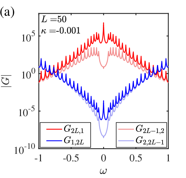
In the main article, we considered a single-band model without topological edge mode, for which the directional amplification comes solely from the continuous band. Here, for completeness, we consider a model with topological edge modes. We show that the zero modes have a visible contribution within a small frequency window when the chain is short, and its effect diminishes as the chain becomes longer. As such, the effect of zero mode is negligible in a long chain.
Specifically, we consider a two-band model introduced in Ref.Song et al. 2019a, with the Bloch Hamiltonian:
| (22) |
The real-space OBC Hamiltonian is
in which
| (29) |
We consider an OBC chain with unit cells, with each unit cell containing two sites (). The odd and even sites correspond to and , respectively. To see the effects of zero modes, we calculate for (Fig. 5). A peak is found at for and . This peak is not seen in and , which is an evidence that it stems from the topological zero modes. In fact, each topological zero mode has a chirality, meaning that it is an eigenstate of . Specifically, the zero modes in our model, as eigenstates of , have vanishing weight at sites and . As such, and are insensitive to the zero modes, which explains the absence of zero-mode peak. A more significant feature is the length dependence of zero-mode peak. Comparing Fig. 5 (a) and (b), or (c) and (d), we see that the zero-mode peak diminishes as the chain length grows. This is intuitive because the effects of topological zero modes are expected to be significant only near the edges.
To compare the numerical results and our theory, we plot , in Fig. 6, which are in excellent agreement with our formulas. Note that is a matrix and are the roots of .
V Periodic-boundary condition
In the main article, we focused on the OBC cases. This is not an arbitrary choice. In fact, it has been pointed out that when the OBC system has directional amplification, the corresponding PBC system tends to be dynamically unstableMcDonald et al. 2018; Wanjura et al. 2020. Moreover, it can be proved that even if dynamical stability is assumed, the PBC Green’s function cannot have exponential growth with increasing spatial distance, and therefore they do not support directional amplification. Since GBZ reduces to the standard BZ in the PBC case, one can prove the absence of exponential growth based on BZ, following Ref. Wanjura et al. 2020.
To prove the absence of exponential growth of with , let us consider a PBC chain of length with site coordinate . The Green’s function reads
| (30) |
where with , as required by the PBC. Defining , we can rewrite it as
| (31) |
where , with . Now we can expand as a Laurent series at the BZ :
| (32) |
We are then able to recast Eq. (31) into
| (33) |
Using the identity , with integer-valued, we have
| (34) |
in which we have made the notational change of integration variable to . The summation over guarantees that , as required by PBC, is satisfied. This expression is quite intuitive. Each value represents the times that a path winds around the chain, the sign of standing for the clockwise/anticlockwise sense. Intuitively, the contributions from larger is less significant, as the rapid phase oscillation of suppress the net contribution.
Taking advantage of the translational symmetry, we can fix and take , then Eq. (34) becomes
| (35) |
We order the roots of as . It follows from the residue theorem that, for ,
| (36) | |||||
and, for ,
| (37) | |||||
where are some numerical coefficients of order unity, and the “” picks up the dominant term in the large limit. Therefore, the -summation in Eq. (35) reads
| (38) |
For large , the term dominates over all terms, while the term dominates all terms, and therefore we only retain these two terms:
| (39) |
Observing that this formula is obtained under the condition , and that , , we see that and . Therefore, the PBC Green’s function cannot have the exponential growth behavior found in the OBC chains.

As an illustration, we show for the model from the main article [Fig. 7]. We find that for all , indicating the absence of exponential growth. This is consistent with the theory. Moreover, we find that the slope of the curve changes at some point on the chain. This behavior can also be seen from the theory. In fact, when the first or second term in Eq. (39) dominates, we have
| (40) |
or
| (41) |
respectively, and the transition point between these two regimes is given by their balance
| (42) |
which leads to . For the parameter values in Fig. 7, we have , which is in accordance with the numerical value.
VI Derivation of the effective non-Hermitian Hamiltonian from the quantum master equation
By the definition of , we have
| (43) |
Inserting the master equation
| (44) |
we obtain
| (45) | |||||
Now we take the Hamiltonian
| (46) |
and the dissipators
| (47) |
with
| (48) |
The specific system shown in Fig. 1(d) of the main article is a special case of this general model. The first term in Eq. (45) is
| (49) |
For the second term in Eq. (45), only the loss dissipators contribute:
| (50) | |||||
while for the third term, only the gain dissipators contribute:
| (51) | |||||
Thus, the second and third terms of Eq. (45) are simplified to
| (52) |
Summing up these terms, Eq. (45) becomes
| (53) |
with the effective non-Hermitian Hamiltonian
| (54) |
For our specific model, the nonzero parameters are , , , , and . It follows from Eq. (54) that the effective non-Hermitian Hamiltonian is given by Fig. 1(a) of the main article. We note that under the OBC, while diagonal elements in the bulk are all , the four edge-site diagonal elements . For simplicity, we let these four elements be , which does not cause any appreciable modification of our main results (While this is intuitively apparent, we have also numerically confirmed it). The operator reads
To simplify the expressions, we measure the frequency with respect to , i.e., shift the frequency (energy) :
We could also include more dissipators such as , and it is straightforward to obtain a similar , except that the diagonal elements become , and become . Our Fig. 1 in the main article corresponds to the special case with other ’s vanishing.