Non-singular vortices with positive mass in 2+1-dimensional Einstein gravity with AdS₃ and Minkowski background

One can solve analytically for the metric in vacuum by setting $f=v$ and $a=n$ identically in Eq. (11) (this eliminates matter from the Lagrangian density (5)). This yields $A^{\prime}(r)=-2r\Lambda$ with solution

where the subscript ‘0’ denotes vacuum. The integration constant $C$ determines the initial conditions at $r=0$. Besides AdS₃ we would also like to study asymptotically Minkowski spacetime ($\Lambda=0$) so in this work we will set $C=1$ (note that this choice also avoids a conical singularity [2, 1]). Substituting the above vacuum solution into Eq. (7) yields $B_{0}(r)=k_{0}\,(-\Lambda r^{2}+C)$ where $k_{0}$ is a positive integration constant which can be absorbed into a redefinition of time. We therefore obtain

In the presence of matter (the vortex), as $r\rightarrow R$, where $R$ is the computational boundary representing formally infinity, we have that $f\rightarrow v$ and $a\rightarrow n$. Using again Eq. (11), the asymptotic form of the metric function $A(r)$ in the presence of matter is²² 2 Outside a core radius $r_{0}$ of the vortex, the mass, the scalar field $f(r)$ and gauge field $a(r)$ hardly change (by less than two percent). Therefore $r_{0}$ sets the scale by which one can compare the computational boundary $R$. In our plots, a conservative value for the core radius is $r_{0}=4$ while the computational boundary is $R=10$. So $R=10$ extends well beyond the core of the vortex in the sense that from $r_{0}=4$ to $R=10$ one is almost entirely in the plateau region where things hardly change. For numerical purposes, we start our plots at $r=0.001$ instead of $r=0$. There are three scales in this problem: a UV scale $\ell_{planck}$ and two IR scales, the AdS radius $\ell_{AdS}$ and $(ev)^{-1}$. For the classical approximation to hold, one requires that $\ell_{AdS}$ and $(ev)^{-1}\gg\,\ell_{planck}$. The radius must be expressed in units of the IR scales. Since $-\Lambda\,R^{2}$ is dimensionless, we can express the radius in units of $\sqrt{-\Lambda}\,\ell_{AdS}$ where $\Lambda$ is a purely negative number e.g. if $\Lambda=-1$ the radius is in units of $\ell_{AdS}$ and if $\Lambda=-3$ the radius is in units of $\sqrt{3}$ $\ell_{AdS}$. One can express $\ell_{AdS}$ in terms of the other IR scale $(ev)^{-1}$. In section 4.1.2 we derive Eq. (32) which is a relation between the IR scale $\ell_{AdS}$ and $v^{-1}$ i.e. $\ell_{AdS}=(q/e)\,v^{-1}$ where the ratio $q/e$ is of order unity and depends on which of the five AdS cases one is considering. For more details and a definition of the parameter $q$, see sections 4.1.2 and 4.2.

where the constant $D$ differs from the constant $C$ in (14). In the next section we will express the mass (ADM mass) of the vortex in terms of $A_{0}(R)$ and $A(R)$.

Using (7) we obtain $B(R)=k\,A(R)$ where the positive integration constant $k$ can no longer be fully absorbed into a redefinition of time (since that has already been done once with the constant $k_{0}$). Therefore, in the presence of matter, at large radius $R$, we have that $B(R)$ is proportional to $A(R)$ but not equal to it.

The spacetime is asymptotically AdS₃, a maximally symmetric spacetime with isometry group $SO(2,2)$. It clearly has a timelike Killing vector since no metric components has a dependence on time. The notion of a conserved energy (the ADM mass) should therefore clearly apply to matter embedded in AdS₃. Maximally symmetric spacetimes can be viewed as the ground states of General Relativity [9] so that it is reasonable to set their energy to be zero. This requires one to subtract out from the Hamiltonian the contribution of the background. This subtraction mechanism is already implemented in the usual formulation of the ADM mass because Minkowski spacetime by itself would otherwise contribute a divergent energy [10]. We can therefore calculate the ADM mass using one of its typical forms [10] suitably generalized to $2+1$ dimensions

where $C_{t}$ is the circle at spatial infinity (i.e. the computational boundary $r=R$), $N(R)=[B_{0}(R)]^{1/2}=[A_{0}(R)]^{1/2}$ is the lapse, $\sigma_{AB}$ is the metric on $C_{t}$, $k$ is the extrinsic curvature of $C_{t}$ embedded on the two-dimensional spatial surface obtained by setting $t$ to be constant in (3) and $k_{0}$ is the extrinsic curvature of $C_{t}$ embedded in the two-dimensional spatial surface of AdS₃. A simple calculation yields

The ADM mass is then given by

As a simple check, if $A(R)=A_{0}(R)$ then $M=0$ so that empty AdS₃ space has zero mass, the expected and desired result. We can simplify the above formula. From Eqs. (14) and (16) we have that $A(R)=-\Lambda R^{2}+D=A_{0}(R)+(D-C)$. At large $R$, $A_{0}(R)>>(D-C)$ so that a binomial expansion of $[A_{0}(R)A(R)]^{1/2}$ at large $R$ yields $A_{0}(R)+\dfrac{1}{2}(D-C)$. We therefore obtain that $M=2\pi\alpha\,(C-D)$. The final expression for the mass in an AdS₃ background is then³³ 3 Eq. 20 is valid when $|A(R)/A_{0}(R)-1|<<1$. This is completely satisfied in all the cases we ran (see values in Table 1). For example, in case I of Table 1, $|A(10)/A_{0}(10)-1|=0.0004$ and the percentage difference between the mass given by Eq. 19 and Eq. 20 is $0.0008\%$. This is such a tiny difference that for all intents and purposes it can be neglected. The advantage of using Eq. 20 over Eq. 19 is that it leads to a more compact and less cumbersome expression for the mass integration formula.

Note that we recover the BTZ black hole spacetime asymptotically. In the BTZ literature [2, 3], $\alpha$ is set to $1/(2\pi)$ and $C$ to zero. We then obtain $D=-M$ so that $A(R)=-\Lambda R^{2}-M$ and $B(R)=k\,A(R)$ which represents the BTZ black hole spacetime asymptotically (the presence of the positive constant $k$ in $B(R)$ has no effect on the spacetime: all curvature scalars are independent of $k$).

The value of $A_{0}(R)=-\Lambda R^{2}+C$ can be calculated analytically for a given $R$. As mentioned earlier, in our work we set $C=1=A_{0}(0)$. The value of $A(r)$ at $r=0$ is not determined by the equations of motion; it is an initial condition. Since $A(r)$ must reduce to $A_{0}(r)$ in the absence of matter, their values must match at the origin. We therefore have $A(0)=A_{0}(0)=C=1$. The quantity $A(R)$ is then obtained by solving the equations of motion numerically and the mass $M$ obtained via Eq.(20). One has reached a large enough value of $R$ when the matter functions $f(r)$ and $a(r)$ reach a nice plateau at the values of $v$ and $n$ respectively and the mass $M$ is stable i.e. that in reducing $R$ in the plateau region, $A_{0}(R)$ and $A(R)$ change but not the value of $M$.

The ADM mass formula (19) applies to asymptotically flat spacetime where $\Lambda=0$. In that case we obtain $A_{0}(R)=C$ and $A(R)=D$ so that

where we used $C=1$. In asymptotically flat spacetime, $A_{0}(r)=B_{0}(r)=1$ (stays constant for all $r$) whereas $A(r)$ starts at unity at $r=0$ and then decreases with $r$ until it reaches a plateau at a positive value of $D$ that is less than unity. The value of $D$ is obtained numerically. Note that formula (21) is in agreement with the angular deficit expected to be produced by localized sources in a $2+1$ dimensional asymptotically flat spacetime⁴⁴ 4 In source free regions, the Einstein equations in $2+1$ dimensions with no cosmological constant yields a locally flat spacetime. Outside localized sources, the spacetime is therefore flat but the topology is that of a cone. This can be seen by rewriting the metric in the source free region in a manifestly flat form and observing that the new angle no longer ranges from $0$ to $2\pi$ but covers a smaller range so that there is an angular deficit. The angular deficit is proportional to the mass of the localized source. [1]. Replacing $\alpha$ by $1/(16\pi G)$, formula (21) reads $D^{1/2}=1-4GM_{flat}$ which is nothing other than the parameter “$\alpha$” (not related to our $\alpha$) found in [1] that determines the angular deficit. If we work in new coordinates $(r^{\prime},\theta^{\prime})$ where $r^{\prime}=r/D^{1/2}$ and $\theta^{\prime}=D^{1/2}\theta$ the two-metric asymptotically takes the flat form $dr^{\prime 2}+r^{\prime 2}\,d\theta^{\prime 2}$ with $\theta^{\prime}$ ranging from $0$ to $2\pi D^{1/2}$ so that there is an angular deficit of

The mass with no gravity in asymptotically flat spacetime, $M_{no-gravity}$, cannot be obtained from comparing two metrics because in this case the metric is fixed throughout to be Minkowski spacetime. However, we derive an integral mass formula for $M_{no-gravity}$ in Appendix A by taking the limit as $\alpha\to\infty$ of $M_{flat}$. The results are reported in the next section.

The second and third equations of motion (12) and (13) can be solved for $A(r)$ in terms of matter fields. This can then be substituted into the first equation (11) to obtain $A^{\prime}(r)$ in term of matter only (see Appendix A). One then obtains the following integral representation for the ADM mass (20) of a vortex embedded in an AdS$3$ background

where $I$ is given by (A.6)

Note that $I$ does not make any reference to metrics, Newton’s constant or the cosmological constant⁵⁵ 5 The function $f(r)$ has dimension of (length)^-1/2 and so does the VEV $v$. The function $a(r)$ is dimensionless. Therefore the integral $I$ has dimensions of (length)^-1 which is the dimension of mass.. It is an integral that is purely over the matter field profiles.

For a vortex under gravity in an asymptotically flat spacetime the integral representation for the ADM mass (21) is given by (A.7)

where

$I$ is the integral given by (24). So $\chi$ is an integral over matter field profiles just like $I$ except that it has a dependence on $\alpha$.

Solving the equations of motion numerically yields the metric and matter field profiles. We can evaluate $M_{AdS_{3}}$ and $M_{flat}$ in two ways: using the metrics or using the matter. In the first method, we extract the asymptotic value of the metric in vacuum and the metric with matter and use the ADM mass formulas (20) and (21) respectively. In the second method one substitutes the matter field profiles into the integral mass formulas (23) and (25) respectively. The two methods must match and this provides a good check on our numerical results.

The first method of extracting values from two separate metrics does not work for the case with no gravity because it takes place in a fixed Minkowski spacetime. However, by taking the limit as $\alpha\to\infty$ of $M_{flat}$ one can derive an integral mass formula that works perfectly well in this case (see Appendix A). The mass of the vortex without gravity given by (A.8) is

where $I$ given by (24) is the same integral that we already encountered for $M_{AdS_{3}}$. Even though we evaluate $M_{AdS_{3}}$ and $M_{no-gravity}$ using the same integral mass formula, the matter field profiles for a vortex under gravity in an AdS₃background will clearly differ from those of a vortex with no gravity in a fixed Minkowski spacetime, leading naturally to different masses.

It is worth noting that in texts that discuss the vortex in fixed Minkowski spacetime (no gravity) they derive from the Hamiltonian an integral expression for the energy of the vortex (label it $I_{no-gravity}$). However, its integrand looks quite different from that of $I$ given by (24). Of course, the two formulas should yield the same mass for the no gravity case and they do. In Appendix B, using the equations of motion for the no gravity case, we show that the integral $I$ can be transformed into the integral $I_{no-gravity}$. It is important to note that $I$ and $I_{no-gravity}$ are not equal at a purely mathematical level. They can be shown to be equal only when the equations of motion for the no gravity case are used. In particular this means that $I$ (and not $I_{no-gravity}$) should be used to calculate the mass for the case of an AdS₃ background.

We can rewrite the integral $I$ given by (24) in a convenient form that reveals more clearly its dependence on the VEV of the scalar field $v$ and the winding number $n$. Since $f(r)$ and $a(r)$ plateau at $v$ and $n$ respectively we can write $f(r)=v\,f_{1}(r)$ and $a(r)=n\,a_{1}(r)$ where $f_{1}(r)$ and $a_{1}(r)$ will always reach asymptotic values of (plateau at) unity. Define $u=\tfrac{e\,v}{n}\,r$. Then $a^{\prime}(r)=e\,va_{1}^{\prime}(u)$, $a^{\prime\prime}(r)=\tfrac{e^{2}\,v^{2}}{n}a_{1}^{\prime\prime}(u)$, $f^{\prime}(r)=\tfrac{e\,v^{2}}{n}\,f_{1}^{\prime}(u)$, $f^{\prime\prime}(r)=\tfrac{e^{2}\,v^{3}}{n^{2}}\,f_{1}^{\prime\prime}(u)$ and $dr=n\,du/(ev)$. Derivatives on functions with subscript ‘1’ are with respect to $u$. Substituting this into (24) yields⁶⁶ 6 The integral $F$ is dimensionless and the dimension of mass stems from $v^{2}$ which has dimensions of (length)^-1. Note that $\lambda/e^{2}$ is dimensionless.

where the integral $F$ is given by

Here $R_{1}=\frac{e\,v}{n}R$ and $F$ is a function of $\lambda/e^{2}$ and a functional of the matter profiles $f_{1}(u)$ and $a_{1}(u)$. The formula (28) does not necessarily imply that $I$ grows exactly quadratically with $v$ and $n$ because the matter profiles that appear in $F$ change with $v$ and $n$. However, since $f_{1}(u)$ and $a_{1}(u)$ always plateau to unity, their change in profile is expected to be limited so that $I$ should still increase significantly if, for example, we double $v$ or $n$. This is what is observed numerically.

Before presenting the numerical results, it is worthwhile to extract a few analytical results from the equations of motion.

For an AdS₃ background, there are six parameters in our numerical simulations: $\lambda$, $\alpha$, $e$, $n$, $v$ and $\Lambda$. We set $\lambda=1$, $\alpha=1$ and $e=3$. We ran numerical simulations for five different cases determined by the values of the three parameters ($n$, $v$, $\Lambda$). The five cases are I=(1,1,-1),II= (1,1,-2),III=(1,1,-3), IV=(1,2,-2) and V=(2,1,-2).

We calculate the mass of the vortex in two ways: first, using the metric together with Eq. (20) and second, inserting the matter profiles into integral (23). The masses are listed in Table 1 and labelled $M_{metric}$ and $M_{integral}$ respectively. The two values match to within two or three decimal places. We know we have reached a large enough $R$ value when the mass is stable (i.e. when we take values of the functions in the plateau region at a radius $r$ much less than $R$ and the mass remains the same). In all cases $R=10$ sufficed⁸⁸ 8 In our plots, the computational boundary was $R=10$ and at that radius the matter functions $f(r)$ and $a(r)$ reached $99.9\%$ of their expected asymptotic values. A computational limitation of our procedure is that our simulation starts at a radius of $r=0.001$ instead of $r=0$. So strictly speaking, we could not implement exactly the boundary conditions at $r=0$ like $f(0)=0$ and $a(0)=0$. However, as mentioned above, the matter functions did reach their expected asymptotic values to within $99.9\%$ so this limitation does not seem to have affected the end results of the simulation in any significant fashion..

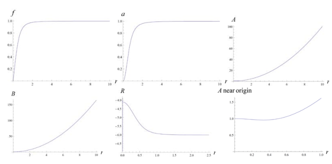
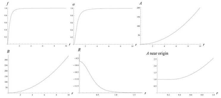
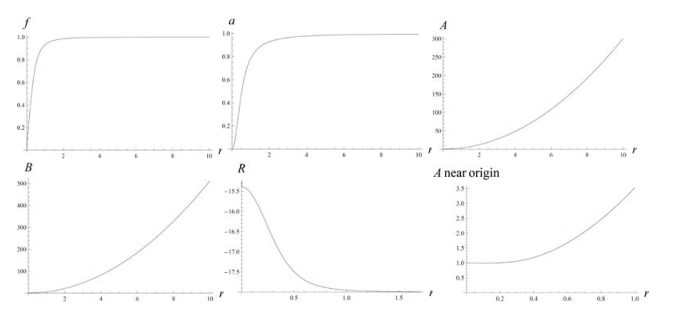
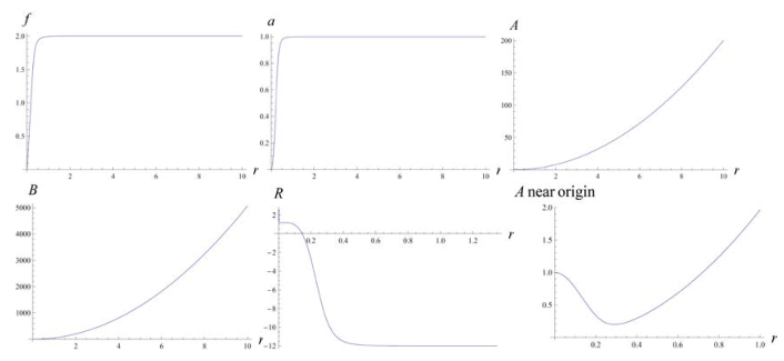
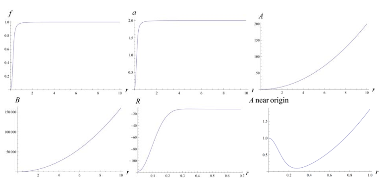
For each of the five cases we plot in figures 1 to 5 below the following functions: the matter functions $f$ and $a$, the metric functions $A$ and $B$ and the Ricci scalar $R$. In all cases, the metric functions $A(r)$ and $B(r)$ are positive throughout so that there is no event horizon. From the Einstein field equations in $2+1$ dimensions, we expect $R$ to plateau at its vacuum value of $6\Lambda$ which is what is observed. We also plot the metric function $A$ near the origin. This is to demonstrate that near the origin and hence in the core of the vortex, $A$ will depart from its “asymptotic” $r^{2}$ dependence. This is particularly pronounced in cases $IV$ and $V$ where $A$ dips significantly below unity near the origin while remaining positive. For these two cases, near the core of the vortex, the metric looks nothing like the BTZ black hole metric. The caption for each of the five figures contains pertinent information besides what we mention below in the text.

Cases $I$, $II$ and $III$ have the same value of $n=1$ and $v=1$ but differ in their value of $\Lambda$ which are $-1$, $-2$ and $-3$ respectively. In Table 1, the mass increases as one goes from case $I$ to case $III$. The vortex is also more compressed when $\Lambda$ is more negative; the value of $r$ at which $f(r)$ reaches $0.9$ are $1.07$, $0.92$ and $0.83$ respectively so that the core of the vortex gets progressively smaller as $\Lambda$ becomes more negative. When matter is compressed it usually gains positive energy so that it makes sense that the mass has increased.

The mass $M=6.53$ of case $IV$ which has $v=2$ and the mass $M=7.14$ of case $V$ with $n=2$ is significantly greater than the mass $M=2.93$ of case $II$ (which has two parameters in common with case $IV$ and case $V$ separately). This is in accord with the $n^{2}v^{2}$ coefficient in the integral mass formula (28). Here case $IV$ and case $V$ are $2.22$ and $2.44$ times more massive than case $II$. As already pointed out at the end of section $3.2$, it is not four times greater because the matter profiles $f_{1}$ and $a_{1}$ that enter (28) change with $v$ and $n$.

We now check how well equation (33) matches the numerical results. We label the $q$ appearing in (33) as $q_{predicted}$. For cases $I$ to $V$ we obtain (quoting numbers sequentially) $q_{predicted}=[3,2.12,1.73,4.24,2.12]$. By taking points asymptotically from the profile of $a$ for each of the five cases and assuming the power law fall off $\epsilon=b/r^{q}$, we can extract $q_{numerical}$. The values are $q_{numerical}=[2.84,2.03,1.68,4.11,2.06]$. We can see that the numbers match quite well (all less than $5.7\%$ difference) so that formula (33) is a reliable predictor of how $a$ behaves asymptotically.

In this subsection we consider vortices under Einstein gravity in $2+1$ dimensions in an asymptotically Minkowski spacetime ($\Lambda=0$). Besides the standard vortex without gravity (fixed Minkowski spacetime) we considered three cases under gravity with different parameters $\alpha=1/(16\pi G)$.

In the no gravity case, where the metric is fixed, we only have the profiles of $f$ and $a$ to plot. Even though its metric is fixed, via a limiting procedure, we were able to obtain the integral mass formula (27) where $I$ is given by (24). The equations of motion are (it is worth rewriting them for the no gravity case as they simplify considerably)

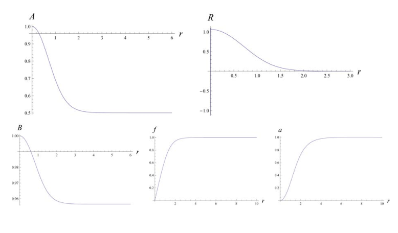
We solve the above equations numerically with the same boundary conditions as (31) (except that $A(0)=1$ is not used since the metric function $A(r)$ does not appear in the equations of motion). The plots (figure 6) are below (the parameters used are $e=1$, $\lambda=1$, $v=1$ and $n=1$). The mass evaluated by inserting the profiles of $f$ and $a$ below into (27) yields $M_{no-gravity}=3.634$. Inserting the same profiles into the standard integral $I_{no-gravity}$ given by (B.1) yields exactly the same value of $3.634$.

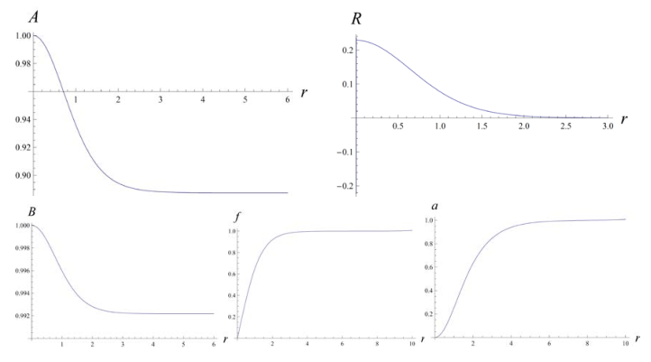
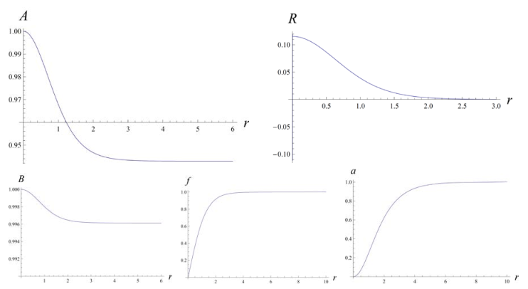
For the case of the vortex under gravity in a Minkowski background we solve the equations of motion (11), (12) and (13) numerically with the boundary conditions (31). The parameters used are: $e=1$, $\lambda=1$, $v=1$, $n=1$ and $\Lambda=0$. We considered three separate cases: $\alpha=1,\alpha=5$ and $\alpha=10$. For each of the three cases we plot the metric function $A$, the Ricci scalar $R$, the metric function $B$ and the matter functions $f$ and $a$. These appear in figures 7, 8 and 9 respectively. Table 2 contains the values of $D$ where the metric function $A$ plateaus, the angular deficit $\delta$ calculated using (22) and converted in degrees, and the masses of the vortex calculated using the metric (Eq. (21)) and the matter profiles (Eq. (25). The mass of the vortex hardly changes with $\alpha$ and hardly differs from the case with no gravity. However, the value of $D$ changes with $\alpha$. This results in an asymptotic conical spacetime where the angular deficit $\delta$ increases significantly as $\alpha$ decreases. There is no singularity at the origin and the Ricci scalar reaches its highest value there before it decreases asymptotically to zero. The value of the Ricci scalar at the origin changes significantly with $\alpha$: it is highest at $\alpha=1$ (R=1.065) and lowest at $\alpha=10$ (R=0.115). We therefore have a smooth spacetime that transitions from a region with curvature at the origin and near the core of the vortex to an asymptotically flat conical spacetime with angular deficit. The curvature at the origin and the angular deficit are highest at $\alpha=1$ and basically five and ten times smaller at $\alpha=5$ and $\alpha=10$ respectively.

References

- [1] S. Deser, R. Jackiw and G. ’t Hooft,Three-Dimensional Einstein Gravity: Dynamics of Flat Space, Ann. of Phys. 152 (1984) 220.
- [2] M. Bañados, C. Tetelboim and J. Zanelli, Black hole in three-dimensional spacetime, Phys. Rev. Lett. 69 (1992) 1849 [arXiv:hep-th/9204099].
- [3] M. Bañados, M. Henneaux, C. Tetelboim and J. Zanelli, Geometry of the 2+1 black hole, Phys. Rev. D 48 (1993) 1506 [arXiv:gr-qc/9302012].
- [4] M. Cadoni, P. Pani and M. Serra, Scalar hairs and exact vortex solutions in 3D AdS gravity, JHEP 01 (2010) 091 [arXiv:0911.3573].
- [5] P. Breitenlohner and D.Z. Freedman, Positive energy in anti-de Sitter backgrounds and gauged extended supergravity, Phys. Lett. B 115 (1982) 197.
- [6] É. Dupuis, Y. Gobeil, B.-H. Lee, W. Lee, R. Mackenzie, M.B. Paranjape, U. A. Yajnik and D.-h. Yeom, Tunneling decay of false vortices with gravitation, JHEP 11 (2017) 028 [arXiv:1709.03839].
- [7] S. R. Coleman and F. De Luccia,Gravitational effects on and of vacuum decay, Phys. Rev. D 21 (1980) 3305.
- [8] J. Oliva, D. Tempo and R. Troncoso, Three dimensional black holes, gravitational solitons, kinks and wormholes for BHT massive gravity, JHEP 07 (2009) 011 [arXiv:0905.1545].
- [9] S.M. Carroll, Spacetime and Geometry, (Pearson Education Inc., San Francisco, CA, 2004).
- [10] E. Poisson, A Relativist’s Toolkit, (Cambridge University Press, Cambridge, UK, 2004).
- [11] E.J. Weinberg, Classical Solutions in Quantum Field Theory, (Cambridge University Press, Cambridge, UK, 2012).
- [12] A. Edery and Y. Nakayama, Gravitating magnetic monopole via the spontaneous symmetry breaking of pure gravity, Phys. Rev. D 98 (2018) 064011 [arXiv:1807.07004].
- [13] A. Ashtekar and A. Magnon, Asymptotically anti-de Sitter spacetimes, Class. Quantum Grav. 1 L39 (1984).
- [14] A. Ashtekar, B. Bonga and A. Kesevan, Asymptotics with a positive cosmological constant: II. Linear fields on de Sitter space-time, Phys. Rev. D 92, 044011 (2015) [arXiv:1506.06152].