Optimizing Over-the-Air Computation in
IRS-Aided C-RAN Systems

Federated learning is an emerging distributed learning paradigm in which mobile devices collaboratively train a machine learning model while preserving the privacy of local data sets [1]. In the presence of latency and bandwidth constraints, the implementation of federated learning on wireless systems is challenging if many workers, or devices, are involved. A potential solution to this problem is over-the-air computation (AirComp), which leverages the superposition property of the multiple access channel (MAC) from worker devices to a parameter server (PS) to allow for simultaneous transmissions from multiple devices [2, 3, 4]. It was reported in [3] that AirComp outperforms a conventional multiple access technique in terms of test accuracy, and that the gain is particularly significant at low transmit power and large number of workers.

AirComp assumes that the wireless channels from different devices can be controlled, e.g., via transmitter-side phase compensation, in order to ensure coherent on-air combining [5]. To alleviate this problem, the work [6] considered a deployment of intelligent reflecting surfaces (IRSs). IRSs, also referred to as reconfigurable intelligent surfaces, can be controlled through integrated electronics in order to shape their response to impinging electromagnetic waves [7]. This enables the modification of the propagation channel between nearby transceivers. As a result, IRSs are considered as a cost-effective solution to improve spectral and energy efficiency of wireless systems [8, 9, 10, 11]. As examples of recent works on IRSs, references [9] and [10] addressed the joint design of downlink beamforming and IRSs’ phases for interference management in multi-user [9] and multi-cell systems [10]. Reference [8] analyzed the number of reflecting elements of IRSs needed to beat conventional wireless relaying techniques (see also [12]). Finally, an information-theoretic study was provided in [13].

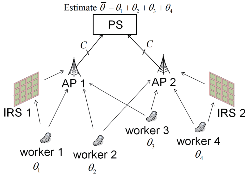
In this work, we study the advantages of deploying IRSs for AirComp systems. Unlike [6], which focused on a MAC channel where workers directly communicate with a PS, we consider the large-scale cloud radio access network (C-RAN) illustrated in Fig. 1, in which the workers upload local models to the PS through distributed access points (APs). The APs, or remote radio heads (RRHs), in C-RAN send the received signals to the PS on fronthaul links. The fronthaul links have finite capacity, requiring fronthaul quantization and compression [14]. We tackle the problem of jointly optimizing the IRSs’ reflecting phases and a linear detector at the PS with the goal of minimizing the mean squared error (MSE) of a parameter estimated at the PS. Due to the non-convexity of the problem, we propose an iterative algorithm that alternately updates the IRSs’ phases and the linear detector. Via numerical results, we validate the advantages of deploying IRSs with optimized phases for AirComp in C-RAN systems.

As illustrated in Fig. 1, we consider an over-the-air computation task performed on a C-RAN system. In the system, $N_{W}$ single-antenna worker devices send locally updated models to a PS through $N_{A}$ single-antenna APs. Each AP is connected to the PS via a fronthaul link, which we model as a digital link of capacity $C$ bit/sample [14]. We define the sets $\mathcal{N}_{W}=\{1,2,\ldots,N_{W}\}$ and $\mathcal{N}_{A}=\{1,2,\ldots,N_{A}\}$ for the workers’ and APs’ indices, respectively.

In this section, we illustrate the operations at the worker devices, the APs, and the PS in the IRS-aided C-RAN system described in Sec. II.

We tackle the problem of jointly optimizing the IRSs’ reflecting phases $\mathbf{v}$ and the linear detection vector $\mathbf{f}$ of the PS with the goal of minimizing the MSE $\mathtt{e}(\mathbf{v},\mathbf{f})$ in (15) while satisfying the unit modulus constraints (13). The problem can be stated as

Since it is difficult to jointly optimize the variables $\mathbf{v}$ and $\mathbf{f}$, we propose an iterative algorithm that alternately optimizes one variable while fixing other.

If we fix the IRSs’ phases $\mathbf{v}$ in problem (16), finding the optimal detector $\mathbf{f}$ becomes an unconstrained quadratic optimization problem, whose closed-form solution is given as

To tackle the problem of optimizing the IRSs’ phases $\mathbf{v}$ for fixed $\mathbf{f}$, we remove the terms that are not dependent on the IRSs’ phases from the cost function. Stating the obtained problem with respect to a stacked vector $\bar{\mathbf{v}}=[\mathbf{v}_{1}^{H}\mathbf{v}_{2}^{H}\cdots\mathbf{v}_{N_{I}}^{H}]^{H}\in\mathbb{C}^{\bar{n}_{I}\times 1}$ with $\bar{n}_{I}=n_{I}N_{I}$ yields

where we have defined the notations $\mathbf{a}_{k}=\bar{\mathbf{H}}_{r,k}^{H}\mathbf{f}\alpha_{k}^{*}\in\mathbb{C}^{\bar{n}_{I}\times 1}$, $b_{k}=\alpha_{k}\mathbf{f}^{H}\mathbf{h}_{d,k}-1$, $\bar{\mathbf{H}}_{r,k}=[\mathbf{H}_{r,1,k}\mathbf{H}_{r,2,k}\cdots\mathbf{H}_{r,N_{I},k}]\in\mathbb{C}^{N_{A}\times\bar{n}_{I}}$, $\mathbf{H}_{r,j,k}=\mathbf{R}_{r,j,k}\mathbf{G}_{j}\text{diag}(\mathbf{h}_{r,j,k})\in\mathbb{C}^{N_{A}\times n_{I}}$, $\mathbf{c}_{i,k}=(P/(2^{C}-1))^{1/2}|\mathbf{f}(i)|\bar{\mathbf{H}}_{r,k}^{H}\mathbf{e}_{i}\in\mathbb{C}^{\bar{n}_{I}\times 1}$, and $d_{i,k}=(P/(2^{C}-1))^{1/2}|\mathbf{f}(i)|\mathbf{e}_{i}^{H}\mathbf{h}_{d,k}$ with $\mathbf{f}(i)$ and $\mathbf{e}_{i}$ being the $i$th element of $\mathbf{f}$ and the $i$th column of an identity matrix of size $N_{A}$, respectively.

The problem (18) is non-convex due to the unit modulus constraints (18c). To handle this issue, we adopt the matrix lifting approach proposed in [6]. Accordingly, we tackle the problem (18) with respect to a matrix $\mathbf{V}\in\mathbb{C}^{(\bar{n}_{I}+1)\times(\bar{n}_{I}+1)}$ defined as

The matrix $\mathbf{V}$ is subject to the constraints $\mathbf{V}\succeq\mathbf{0}$, $\text{rank}(\mathbf{V})\leq 1$, and $\mathbf{V}(m,m)=1$ for all $m\in\{1,2,\ldots,\bar{n}_{I}+1\}$. From $\mathbf{V}$, the IRSs’ phase vector $\bar{\mathbf{v}}$ can be recovered as the first $\bar{n}_{I}$ elements of the last column of $\mathbf{V}$.

We tackle (18) with respect to $\mathbf{V}$ by using the following equalities:

Specifically, by substituting (IV) and (IV) into problem (18), we obtain the problem

with the matrix $\mathbf{M}$ defined as

To address the non-convexity of constraint (35c), we note that (35c) is equivalent to the constraint [6]

where $\sigma_{1}(\cdot)$ denotes the largest singular value of the input matrix. Function $\sigma_{1}(\mathbf{V})$ is convex in $\mathbf{V}$ [18]. Furthermore, for $\mathbf{V}\succeq\mathbf{0}$, the left-hand side (LHS) of (40) is 0 when $\text{rank}(\mathbf{V})\leq 1$ and it becomes larger than 0 otherwise.

Based on this observation, as in [6], we tackle the problem

with a fixed weight $\gamma\geq 0$. In problem (41), we have removed the rank constraint (35c) and instead added a penalty term $\gamma(\text{tr}(\mathbf{V})-\sigma_{1}(\mathbf{V}))$ to the cost function that increases if (35c) is not satisfied.

The problem (41) is a difference-of-convex (DC) problem whose locally optimal solution can be efficiently found via the concave convex procedure (CCP) approach [19]. CCP solves a sequence of convex problems obtained by linearizing the terms that induce non-convexity. In the DC problem (41), the only term that induces non-convexity is $-\gamma\cdot\sigma_{1}(\mathbf{V})$ in the penalty term. Linearizing $-\gamma\cdot\sigma_{1}(\mathbf{V})$ at a reference point $\mathbf{V}=\mathbf{V}^{\prime}$ yields the upper bound [6]

where $\mathbf{u}_{1}(\cdot)$ returns the eigenvector of the input matrix corresponding to the largest eigenvalue. The condition (42) is satisfied with equality when $\mathbf{V}=\mathbf{V}^{\prime}$. The CCP based algorithm for optimizing $\mathbf{V}$ is summarized in Algorithm 1.

Overall, the proposed algorithm that alternately optimizes the IRSs’ phases $\mathbf{v}$ and the linear detector $\mathbf{f}$ is detailed in Algorithm 2. In the algorithm, we initialize $\mathbf{v}$ and $\mathbf{f}$ in Steps 1-2, and update $\mathbf{v}$ for fixed $\mathbf{f}$ in Steps 3-4. In Step 4, $\mathbf{v}$ is modified only when it does not satisfy the modulus constraints (18c). In Step 5, $\mathbf{f}$ is updated for fixed $\mathbf{v}$, and we check the convergence in Step 6.

In simulation, we assume that the positions of $N_{W}$ workers, $N_{A}$ APs and $N_{I}$ IRSs are uniformly distributed in a circular area of radius 100 m. We set the variance of local parameters to $\sigma_{\theta,k}^{2}=1$ for $k\in\mathcal{N}_{W}$ and assume $c_{0}=20$ dB, $\eta=3$ in the path-loss models and $\gamma=1$ for the penalty coefficient in (41a). For all links, we consider independent Rayleigh fading channels that are distributed as $h_{d,i,k}\sim\mathcal{CN}(0,1)$, $\mathbf{g}_{i,j}\sim\mathcal{CN}(\mathbf{0},\mathbf{I})$ and $\mathbf{h}_{r,j,k}\sim\mathcal{CN}(\mathbf{0},\mathbf{I})$. We compare the performance of the proposed optimized scheme with two baseline schemes, one without IRSs and one with IRSs whose reflecting phases are randomly chosen. In all figures, we plot the normalized MSE, which is defined as the MSE $\mathtt{e}(\mathbf{v},\mathbf{f})$ normalized by $\mathtt{E}[|\bar{\theta}|^{2}]$ so that it lies in the range $[0,1]$.

In Fig. 2, we plot the average normalized MSE versus the fronthaul capacity $C$ for an IRS-aided C-RAN system with $N_{W}=10$, $N_{A}=5$, $N_{I}=2$, $n_{I}=10$ and $P/\sigma_{z}^{2}\in\{5,20\}$ dB. The figure shows that the proposed optimized scheme outperforms both baseline schemes without IRS and with random phases, and that the gain increases with the fronthaul capacity $C$. This is because, when $C$ is small, the impact of carefully designing the IRSs’ phases becomes minor due to the impact of the quantization noise signals $\{q_{i}\}_{i\in\mathcal{N}_{A}}$. Also, the gain increases with the signal-to-noise ratio (SNR) $P/\sigma_{z}^{2}$ of the uplink channel, and this trend coincides with the observation reported in [10, Sec. IV].

Fig. 3 plots the average normalized MSE versus the number $N_{A}$ of APs for an IRS-aided C-RAN system with $N_{W}=5$, $N_{I}=2$, $n_{I}\in\{20,50\}$, $C=5$ and $P/\sigma_{z}^{2}=10$ dB. When there are only a few APs, deploying IRSs provides relevant gains only when the reflecting phases are optimized according to Algorithm 2. However, the impact of optimizing the reflecting phases becomes minor for sufficiently large $N_{A}$.

We have studied the impacts of deploying IRSs on AirComp in a C-RAN system. To this end, we have tackled the joint optimization of the IRSs’ reflecting phases and the linear detector at the PS with the goal of minimizing the MSE of the parameter estimated at the PS. Numerical results were provided that investigate the effects of various parameters on the performance gain of the proposed optimization scheme compared to baseline schemes. Among open problems, we mention the design of channel estimation process, the investigation of the effect of imperfect CSI, and the design of AirComp jointly with information transfer.

References

- [1] K. Bonawitz and et al, ”Towards federated learning at scale: System design,” arXiv:1902.01046, Feb. 2019.
- [2] B. Nazer and M. Gastpar, ”Computation over multiple-access channels,” IEEE Trans. Inf. Theory, vol. 53, no. 10, pp. 3498–3516, Oct. 2007.
- [3] M. M. Amiri and D. Gunduz, ”Machine learning at the wireless edge: Distributed stochastic gradient descent over-the-air,” in Proc. IEEE ISIT2019, Paris, France, Jul. 2019, pp. 1–5.
- [4] K. Yang, T. Jiang, Y. Shi, and Z. Ding, ”Federated learning via over-the-air computation,” IEEE Trans. Wireless Commun., vol. 19, no. 3, pp. 2022–2035, Mar. 2020.
- [5] T. Sery and K. Cohen, ”On analog gradient descent learning over multiple access fading channels,” arXiv:1908.07463, Aug. 2019.
- [6] T. Jiang and Y. Shi, ”Over-the-air computation via intelligent reflecting surfaces,” in Proc. IEEE Globecom 2019, Waikoloa, USA, Dec. 2019.
- [7] E. Basar, M. D. Renzo, J. D. Rosny, M. Debbah, M. Alouini, and R. Zhang, ”Wireless communications through reconfigurable intelligent surfaces,” IEEE Access, vol. 7, pp. 116753–116773, 2019
- [8] E. Bjornson, O. Ozdogan, and E. G. Larsson, ”Intelligent reflecting surface vs. decode-and-forward: How large surfaces are needed to beat relaying?,” arXiv:1906.03949, Jun. 2019.
- [9] Q. Wu and R. Zhang, ”Intelligent reflecting surface enhanced wireless network via joint active and passive beamforming,” IEEE Trans. WirelessCommun., vol. 18, no. 11, pp. 5394–5409, Nov. 2019.
- [10] C. Pan, H. Ren, K. Wang, W. Xu, A. Nallanathan, M. Elkashlan, and L. Hanzos, ”Multicell MIMO communications relying on intelligent reflecting surface,” arXiv:1907.10864, Jul. 2019.
- [11] M. Di Renzo and et al, ”Smart radio environments empowered by reconfigurable ai meta-surfaces: an idea whose time has come,” EURASIP J. Wireless Commun. Netw., pp. 1–20, May 2019.
- [12] K. Ntontin and et al, ”Reconfigurable intelligent surfaces vs. relaying: Differences, similarities, and performance comparison,” arXiv:1908.08747, Aug. 2019.
- [13] R. Karasik, O. Simeone, M. Di Renzo, and S. Shamai, “Beyond max-SNR: Joint encoding for reconfigurable intelligent surfaces,” arXiv:1911.09443, Nov. 2019.
- [14] S.-H. Park, O. Simeone, O. Sahin, and S. Shamai, ”Fronthaul compression for cloud radio access networks: Signal processing advances inspired by network information theory,” IEEE Signal Process. Mag., vol. 31, no. 6, pp. 69–79, 2014.
- [15] X. Cao, G. Zhu, J. Xu, and K. Huang, ”Optimal power control for over-the-air computation in fading channels,” arXiv:1906.06858, Jun. 2019.
- [16] R. Zamir and M. Feder, ”On lattice quantization noise,” IEEE Trans.Inf. Theory, vol. 42, no. 4, pp. 1152–1159, Jul. 1996.
- [17] A. E. Gamal and Y.-H. Kim, Network Information Theory, Cambridge Univ. Press, 2011.
- [18] S. Boyd and L. Vandenberghe, Convex Optimization, Cambridge Univ. Press, 2004.
- [19] M. Tao, E. Chen, H. Zhou, and W. Yu, ”Content-centric sparse multicast beamforming for cache-enabled cloud RAN,” IEEE Trans. Wireless Commun., vol. 15, no. 9, pp. 6118–6131, 2016.