Detection loophole in measurement-device-independent entanglement witness

Quantum mechanics provides description for physical systems in terms of quantum states belonging to some Hilbert space. One of the distinguishing features of composite quantum systems is the presence of a kind of correlation between different subsystems, called entanglement HHHH; das'06; toth'09. Presence of entanglement enables better efficiencies of various tasks like quantum teleportation bennett'93, quantum dense coding bennett'92, and entanglement-based quantum cryptography ekert'91. Therefore, it is of importance to know whether a state is entangled. Over the years, several methods have been proposed to detect entanglement, and to name a few, there are the positive partial transpose criterion peres'96; horodecki'96, range criterion horedecki'97, violation of Bell inequality bell, and negativity of the expectation values of entanglement witness (EW) operators horodecki'96; terhal'00. Several such procedures have also been used to verify entanglement in laboratories exp1.

The method of entanglement witnesses has gained importance over the years as an efficient detector of entanglement of shared quantum states. If one has some a priori information about a shared quantum state, then an EW may be constructed for that state. It is also possible to implement such a method in a laboratory as the expectation value of any EW can be obtained by performing local measurements on subsystems constituting the composite system. Still, an imperfect implementation of the measurements may wrongly indicate a separable state to be entangled witness1, just as a “local” state may appear to violate a Bell inequality loophole-BI. Negativity of the expectation value of any entanglement witness operator guarantees entanglement, when the measurement devices involved are ideal. There are at least two possible ways by which realistic measurements can drive the process away from its ideal variety. Firstly, the intended measurement basis may get altered (“wrong” measurements) and secondly, the detectors used can be noisy (“imprecise” measurements). EWs are prone to both these “defects”. Both pose challenges to an experimentalist, as defective measurements can lead to false positives in witnessing entanglement. The concept of measurement-device-independent entanglement witnesses (MDI-EWs) was introduced to address the first problem Cyril'13. It was shown that an MDI-EW can always be constructed from a standard EW, based on a semi-quantum nonlocal game, where every entangled state provides advantage over all separable states Buscemi'12. Robustness of MDI-EWs as compared to that of standard ones, for sequential witnessing of entanglement was analyzed in srivastava.

In this article, we focus on the second problem, which involves imprecise measurements due to noisy detectors. Any of the entanglement detection methods, if performed with imprecise measurements, can lead to erroneous observations. By “imprecise measurements”, we mean here that the corresponding measurement devices have non-unit efficiency, arising due to loss of measurement outcomes. Such studies are usually clustered into what is referred to as the “detection loophole” problem, as the task is to detect entanglement with non-ideal measurement devices. The problem of detection loophole for Bell inequality violations has been studied extensively, both theoretically loophole-BI as well as experimentally BIexp. In the context of entanglement witnesses, the detection loophole problem was analyzed recently in witness1; witness2.

The purpose of MDI-EWs is to remove the measurement-device-dependence of EWs, i.e., to guarantee entanglement of a shared quantum state, independent of what measurements are being performed. But whether this type of witness also guarantees entanglement, independent of the possibly non-unit efficiencies of the corresponding measurement devices, is yet to be answered. In this article, we analyze the detection loophole present in MDI-EWs considering such non-ideal measurement devices. To be specific, we consider the problem in three scenarios. The first one involves the losses in the detector, whereas the second considers the additional counts (“dark counts”) therein. We finally consider a third scenario, where both these kinds of detector inefficiencies can be present. In the case of lossy detectors, having a certain non-unit efficiency, we provide an upper bound on the measured value of the MDI-EW function which is sufficient to certify entanglement. In case of additional counts, we observe that MDI-EWs do not guarantee entanglement falsely, whatever be the detector’s efficiency. We finally derive a relation for loophole-free detection of entanglement using a MDI-EW in presence of both types of detector inefficiencies. We illustrate the results by using Werner states Werner and noisy Greenberger-Horne-Zeilinger (GHZ) states gange-Dheu-khele-jai.

This paper is organized as follows. In Sec. II, we discuss about the detection loophole in case of standard EWs. In Sec. III, a brief description on MDI-EWs is given. The detection loophole in case of MDI-EWs is analyzed in Sec. IV. A short summary is provided in Sec.V.

In this section, we briefly discuss about EWs and ways of overcoming the detection loophole in the process of measuring expectation values corresponding to an EW witness1. A hermitian operator, $W$, is called an EW of a certain shared system, if and only if tr$(W\sigma)\geq 0$ for all separable states $\sigma$ of that system and there exists at least one entangled state $\rho_{e}$ such that tr$(W\rho_{e})<0$. It can be seen that for every entangled state, $\rho_{e}$, there exists at least one witness operator, $W$, which satisfies the above conditions and can detect that $\rho_{e}$ horodecki'96. Let us mention two examples of witness operators. We know that the Werner state Werner, $\rho_{p}=p|\psi^{-}\rangle\langle\psi^{-}|+\frac{1-p}{4}\mathbb{I}_{4}$, where $|\psi^{-}\rangle=\frac{1}{\sqrt{2}}(|01\rangle-|10\rangle)$ and $0\leq p\leq 1$, is entangled for $p>\frac{1}{3}$, with $\{|0\rangle,|1\rangle\}$ being the eigenbasis of the Pauli $\sigma_{z}$ operator, as ensured by the partial transposition criterion peres'96; horodecki'96. Here, $\mathbb{I}_{k}$ denotes the identity operator on a complex Hilbert space of dimension $k$. For $p>\frac{1}{3}$, the operator $\rho_{p}^{\text{T}_{B}}$ will have one negative eigenvalue neg. Here, the superscript $\text{T}_{B}$ denotes transposition on the second system. The eigenvector corresponding to this negative eigenvalue, viz. $\frac{1}{4}(1-3p)$, is $|\phi^{+}\rangle=\frac{1}{\sqrt{2}}(|00\rangle+|11\rangle)$. Then a witness operator that can detect the state $\rho_{p}$ can be considered to be of the form horodecki'96; terhal'00

$$W_{\rho_{p}}=|\phi^{+}\rangle\langle\phi^{+}|^{T_{B}}.$$

(1)

Another example can be given by considering 3-qubit noisy GHZ states, $\rho_{q}^{GHZ}=q|GHZ\rangle\langle GHZ|+\frac{1-q}{8}\mathbb{I}_{8}$, where $|GHZ\rangle=\frac{1}{\sqrt{2}}(|000\rangle+|111\rangle)$ gange-Dheu-khele-jai and $0\leq q\leq 1$. This state can be shown to be genuinely tripartite entangled for $q>\frac{3}{7}$ ref1. A witness operator which can detect genuine tripartite entanglement of $\rho_{q}^{GHZ}$ is given by toth'09; ref2

$$W_{\rho_{q}^{GHZ}}=\frac{1}{2}\mathbb{I}_{8}-|GHZ\rangle\langle GHZ|.$$

(2)

But, due to existence of the detection loophole in measurement processes, one may mistakenly identify a separable state, say $\sigma^{\prime}$, as an entangled state, i.e, one may get tr$\left(W\sigma^{\prime}\right)<0$, where $W$ is the corresponding entanglement witness. The condition for overcoming the detection loophole for entanglement witnesses was first discussed by Skwara et al. witness1. Since we can always decompose a hermitian operator, acting on a tensor product Hilbert space, $\mathcal{H}_{1}\otimes\mathcal{H}_{2}\ldots\otimes\mathcal{H}_{n}$, in terms of the identity operator, $\mathbb{I}$, of the total Hilbert space and traceless hermitian operators, $S_{\alpha}$, as products of hermitian operators operating on local subspaces $\mathcal{H}_{1}$, $\mathcal{H}_{2}$, $\cdot\cdot\cdot$, $\mathcal{H}_{n}$, we can write an $n$-partite witness operator as

$$W=C_{0}\mathbb{I}+\sum_{\alpha}C_{\alpha}S_{\alpha},$$

(3)

where $C_{0}$ and $C_{\alpha}$ are real numbers. Now, an expectation value of $W$ depends on the individual expectation values of $S_{\alpha}$. The measured expectation value of $S_{\alpha}$ for a state $\rho$ is given by $\langle S_{\alpha}\rangle_{m}=\frac{\sum_{i}n_{i}\lambda_{i}}{N}$, where $n_{i}$ denotes the number of times the eigenvalue $\lambda_{i}$ has clicked and $N=\sum_{i}n_{i}$. But due to additional and lost events in the measurement process, this value could be different from the true expectation value of $S_{\alpha}$ given by $\langle S_{\alpha}\rangle_{t}=\frac{\sum_{i}\tilde{n_{i}}\lambda_{i}}{\tilde{N}}$. Here $\tilde{n_{i}}$ denotes number of times $\lambda_{i}$ should have clicked in the case of ideal detectors and $\tilde{N}=\sum_{i}\tilde{n_{i}}$. Let the number of additional and lost events for $\lambda_{i}$ be $\epsilon_{+i}$ and $\epsilon_{-i}$ respectively, and set $\sum_{i}\epsilon_{\pm i}=\epsilon_{\pm}$. The additional and lost event efficiencies are defined as $\eta_{+}=\frac{\tilde{N}}{\tilde{N}+\epsilon_{+}}$ and $\eta_{-}=\frac{\tilde{N}-\epsilon_{-}}{\tilde{N}}$.

In this paper, we consider the following three cases separately. In the first case (Case 1), the additional event efficiency (i.e. $\eta_{+}$) is taken to be unity, with the lost event efficiency (i.e. $\eta_{-}$) being kept arbitrary. In the next case (Case 2), keeping $\eta_{-}=1$, we consider arbitrary $\eta_{+}$. Finally, in the third case (Case 3), we consider the general case of arbitrary additional and lost event efficiencies. In all the cases, $\epsilon_{\pm i}$’s are taken to be independent of $i$, say $\overline{\epsilon}_{\pm}$.

Case 1: For the first case, we get $\langle S_{\alpha}\rangle_{m}=\frac{\sum_{i}\left(\tilde{n}-\overline{\epsilon}_{-}\right)\lambda_{i}}{\tilde{N}-\epsilon_{-}}=\left(\frac{\sum_{i}\tilde{n_{i}}\lambda_{i}}{\tilde{N}}-\frac{\overline{\epsilon}_{-}\sum_{i}\lambda_{i}}{\tilde{N}}\right)\frac{\tilde{N}}{\tilde{N}-\epsilon_{-}}$. Since $S_{k}$ are traceless matrices, we get $\langle S_{\alpha}\rangle_{m}=\frac{\langle S_{\alpha}\rangle_{t}}{\eta_{-}}$. Hence using Eq. (3), we get the relation between measured and true values of $W$ as

	$\displaystyle\langle W\rangle_{m}$	$\displaystyle=$	$\displaystyle C_{0}+\sum_{\alpha}C_{\alpha}\frac{\langle S_{\alpha}\rangle_{t}}{\eta_{-}}$
		$\displaystyle=$	$\displaystyle C_{0}\left(1-\frac{1}{\eta_{-}}\right)+\frac{\langle W\rangle_{t}}{\eta_{-}}.$

Now, as we mentioned before, $W$ will detect entanglement of a state $\rho$ when $\langle W\rangle_{t}<0$, where the expectation value is taken over the state $\rho$. Hence, even in the presence of detection loophole, $W$ can detect the entanglement of $\rho$ correctly when the following inequality is satisfied:

$$\langle W\rangle_{m}<C_{0}\left(1-\frac{1}{\eta_{-}}\right).$$

(4)

As the completely depolarized state is a separable state, we must have $C_{0}>0$. Therefore, $C_{0}\left(1-\frac{1}{\eta_{-}}\right)<0$ for $\eta_{-}\neq 1$. States for which $C_{0}\left(1-\frac{1}{\eta_{-}}\right)\leq\langle W\rangle_{m}<0$, a negative $\langle W\rangle_{m}$ will not be sufficient for the experimentalist to infer entanglement in the shared state. If we consider the two examples of witness operators that we considered above, viz. the conditions for Werner state ($W_{\rho_{p}}$) and noisy GHZ state ($W_{\rho_{q}^{GHZ}}$), we get the conditions

	$\displaystyle\langle W_{\rho_{p}}\rangle_{m}<\frac{1}{4}\left(1-\frac{1}{\eta_{-}}\right)\text{ and}$
	$\displaystyle\langle W_{\rho_{q}^{GHZ}}\rangle_{m}<\frac{3}{8}\left(1-\frac{1}{\eta_{-}}\right),$

for loophole-free detection of entanglement in the corresponding states, in the case when the lost event efficiency is non-ideal. Hence, for example, if the lost event efficiency is $\eta_{-}=\frac{1}{2}$, then the witness operator, $W_{\rho_{p}}$, can detect an entangled Werner state if $\langle W_{\rho_{p}}\rangle_{m}<-\frac{1}{4}$ is satisfied, and $W_{\rho_{q}^{GHZ}}$ can detect an entangled noisy GHZ state if $\langle W_{\rho_{q}^{GHZ}}\rangle_{m}<-\frac{3}{8}$ is satisfied.

Case 2: Doing similar calculations for the second case, we get

$$\langle W\rangle_{m}=C_{0}\left(1-\eta_{+}\right)+\eta_{+}\langle W\rangle_{t}.$$

(5)

Here, $C_{0}\left(1-\eta_{+}\right)\geq 0$. Hence $\langle W\rangle_{t}\leq\langle W\rangle_{m}$ for all values of $\eta_{+}$. Therefore, in this case, even though lesser states will be detected using $W$, we will never identify a separable state as an entangled state. Hence, EW is robust under the second kind of loophole.

Case 3: Let us now move to the general case where the additional event efficiency, $\eta_{+}$, as well as the lost event efficiency, $\eta_{-}$, are both at non-unit values. The condition on the measured expectation value of witness function, $\langle W\rangle_{m}$, which guarantees entanglement, even in the presence of non-ideal $\eta_{\pm}$, is given by

$$\langle W\rangle_{m}<C_{0}\left(1-\frac{1}{\eta_{-}+\frac{1}{\eta_{+}}-1}\right).$$

(6)

Notice that $\eta_{-}=1$ or $\eta_{+}=1$ lead us to the previously obtained relations.

Any entanglement witness operator can always be expanded in a basis consisting of tensor products of local hermitian operators. Expectation value of a witness operator in any given quantum state can therefore be obtained by performing measurements in the bases of those local hermitian operators. However, if an experimentalist performs a measurement that is different from what is required to evaluate the expectation value of the witness operator in a given state, then a negative expectation value does not guarantee that the state is entangled. Therefore, Branciard et al. Cyril'13 came up with the idea of measurement-device-independent entanglement witnesses (MDI-EWs) which guarantee the entanglement of a quantum state, i.e., it never indicates a separable state to be entangled, independent of the measurements that are actually performed. Moreover, it was also observed that when effect of lossy detectors is to modify joint probabilities by the same multiplicative factor, then MDI-EWs can still do its job properly Cyril'13.

In this section, we briefly discuss the MDI-EWs studied in Cyril'13, motivated by the “nonlocal semi-quantum game” presented in Buscemi'12. Let $W$ be an entanglement witness operator acting on the Hilbert space $\mathcal{H}_{A}\otimes\mathcal{H}_{B}$, with the dimension of $\mathcal{H}_{A}$ being $d_{A}$ and that of $\mathcal{H}_{B}$ being $d_{B}$. Consider complete sets of density matrices, $\{\tau_{r}|~r=1,2,\ldots,d_{A}^{2}\}$ acting on $\mathcal{H}_{A}$ and $\{\omega_{s}|~s=1,2,\ldots,d_{B}^{2}\}$ acting on $\mathcal{H}_{B}$. These sets are “complete” in the sense that they span the space of hermitian matrices on the corresponding Hilbert spaces ($\mathcal{H}_{A}$ or $\mathcal{H}_{B}$) with respect to the field of reals. One can always find a set of real numbers, ${\beta_{rs}}$, such that any entanglement witness can be expanded as

$$W=\sum_{rs}\beta_{rs}\tau_{r}^{\text{T}}\otimes\omega_{s}^{\text{T}},$$

(7)

where the superscript, T, over the states denotes their transposes. The above equation is a consequence of the existence of a set of density matrices which span the space of hermitian operators. Note that the expansion in Eq. (7) is not unique.

Consider two parties Alice $(A)$ and Bob $(B)$ sharing a quantum state $\rho_{AB}$ acting on $\mathcal{H}_{A}\otimes\mathcal{H}_{B}$. Let $A$ and $B$ be provided the set of states $\{\tau_{r}\}$ and $\{\omega_{s}\}$ as their auxiliary quantum inputs, respectively.

Each party then performs a joint dichotomic measurement, $\{|\Phi_{A(B)}^{+}\rangle\langle\Phi_{A(B)}^{+}|,~\mathbb{I}_{d_{A(B)}^{2}}-|\Phi_{A(B)}^{+}\rangle\langle\Phi_{A(B)}^{+}|\}$, on their part of the shared state $\rho_{AB}$ and their respective inputs. Here $|\Phi_{A(B)}^{+}\rangle=\frac{1}{\sqrt{d_{A(B)}}}\sum_{i=0}^{d_{A(B)}-1}|ii\rangle$, whereas $\{|i\rangle\}$ forms the computational basis. For simplicity of notations, the outcomes $|\Phi_{A(B)}^{+}\rangle\langle\Phi_{A(B)}^{+}|$ will be indicated as ‘1’, and $\mathbb{I}_{d_{A(B)}^{2}}-|\Phi_{A(B)}^{+}\rangle\langle\Phi_{A(B)}^{+}|$ will be indicated as ‘0’. The joint probability of $A$ getting an outcome $a$ given $\tau_{r}$ as the quantum input, and $B$ getting an outcome $b$ given $\omega_{s}$ as the quantum input is denoted by $P(a,b|\tau_{r},\omega_{s})$. The MDI-EW function is then given by

$$I(\rho_{AB})=\sum_{r,s}\beta_{rs}P(1,1|\tau_{r},\omega_{s}).$$

(8)

The connection between the MDI-EW function, $I(\rho_{AB})$, and the entanglement witness, $W$, can be obtained with the help of Eq. (7), and is given by Cyril'13

$$I(\rho_{AB})=\frac{\text{tr}(W\rho_{AB})}{d_{A}d_{B}},$$

(9)

where $\rho_{AB}$ is the shared state whose entanglement detection is in process. The MDI-EW function thus satisfies all the properties of an entanglement witness operator.

Suppose now that $A$ and $B$ share a separable state and let instead of performing the POVM, $\{|\Phi_{A(B)}^{+}\rangle\langle\Phi_{A(B)}^{+}|,~\mathbb{I}_{d_{A(B)}^{2}}-|\Phi_{A(B)}^{+}\rangle\langle\Phi_{A(B)}^{+}|\}$, $A$ performs an arbitrary two-outcome POVM, $\{A_{0},~A_{1}\}$, and $B$ performs an arbitrary two-outcome POVM, $\{B_{0},~B_{1}\}$, to construct the MDI-EW function for that separable state. It turns out that the MDI-EW function for any separable state still remains positive, i.e., $I(\sigma_{AB})\geqslant 0$, for all $\sigma_{AB}$ belonging to the space of separable states, thus justifying the “measurement-device-independent” adjective of MDI-EWs.

To formulate a MDI-EW for detecting genuine multipartite entanglement (GME), one can use the following decomposition of a witness operator,

$$W_{\rho_{q}^{GME}}=\sum_{r,s,u}\beta_{rsu}\tau_{r}^{\text{T}}\otimes\omega_{s}^{\text{T}}\otimes\gamma_{u}^{\text{T}},$$

(10)

where $W_{\rho_{q}^{GME}}$ is known to detect the GME of a three-party state $\rho_{GME}$. In this case, the three parties, say Alice, Bob, and Charlie, share the state $\rho_{GME}$ and have $\tau_{r}$, $\omega_{s}$, $\gamma_{u}$ as their auxiliary quantum inputs, and the witness operator acts on the joint Hilbert space of Alice, Bob, and Charlie, which are, say $\mathcal{H}_{A}$, $\mathcal{H}_{B}$, and $\mathcal{H}_{C}$ respectively. Hence, the corresponding MDI-EW is given by Cyril'13

$$I(\rho_{GME})=\sum_{r,s,u}\beta_{rsu}P(1,1,1|\tau_{r},\omega_{s},\gamma_{u}).$$

(11)

In the bipartite case, the witness operator, given in Eq. (1), which can detect entanglement of the Werner state, can be decomposed in the form of Eq. (7), where $\beta_{rs}$, $\tau_{r}$, and $\omega_{s}$ are given by Cyril'13

	$\displaystyle\beta_{rs}=\frac{5}{8}\text{ for $r=s$, \ \ \ \ \ \ \ \ \ }\beta_{rs}=-\frac{1}{8}\text{ for $r\neq s$},$
	$\displaystyle\tau_{r}=\sigma_{r}\frac{\mathbb{I}_{2}+\vec{n}\cdot\vec{\sigma}}{2}\sigma_{r},\text{ \ \ \ \ \ \ \ \ \ }\omega_{s}=\sigma_{s}\frac{\mathbb{I}_{2}+\vec{n}\cdot\vec{\sigma}}{2}\sigma_{s}.$		(12)

Here $r$ and $s$ run from 0 to 3, $\vec{n}=\frac{1}{\sqrt{3}}(1,1,1)$, and $\vec{\sigma}=(\sigma_{1},\sigma_{2},\sigma_{3})$, i.e., the Pauli spin matrices and $\sigma_{0}=\mathbb{I}_{2}$. Hence, the corresponding MDI-EW can be constructed as Cyril'13

$$I(\rho_{p})=\frac{5}{8}\sum_{s=t}P(1,1|\tau_{r},\omega_{s})-\frac{1}{8}\sum_{s\neq t}P(1,1|\tau_{r},\omega_{s}).$$

Similarly, the witness operator for the noisy GHZ state, given in Eq. (2), can be decomposed as in Eq. (10). We chose the same $\tau_{r}$ and $\omega_{s}$ as in Eq. (12) and determined the corresponding $\gamma_{u}$. In this particular decomposition, the coefficients $\beta_{r,s,u}$ are given by Cyril'13

	$\displaystyle\beta_{rsu}=\frac{3}{32}$		$\displaystyle\left(-1\right)^{\left[(r-1)/2\right]\left[(s-1)/2\right]+\left[(r-1)/2\right]\left[(u-1)/2\right]+\left[(s-1)/2\right]\left[(u-1)/2\right]+1}$
	$\displaystyle\times$		$\displaystyle\left(-1\right)^{\left[(r-1)/2\right]+\left[(s-1)/2\right]+\left[(u-1)/2\right]}+\left(-1\right)^{r+s+u}\sqrt{3}.$

Using this $\beta_{rsu}$ in Eq. (11), the MDI-EW can be determined and used in experiments.

As discussed in the preceding section, the value of an MDI-EW, independent of the POVM performed on the joint state, $\tau_{r}\otimes\sigma_{AB}\otimes\omega_{s}$, is always non-negative for all separable states, $\sigma_{AB}$. Now the question is whether it is also robust in the presence of detection inefficiencies. In other words, we ask: even if the detection efficiencies, defined in Sec. II, are not unit, will $I(\sigma_{AB})\geq 0$ hold for all separable states? In this section, we explore this question, find that a detection loophole is, in principle, also present in this measurement-device-independent scenario, and derive the condition for closing the detection loophole. In the first case (Case I), we take the additional event efficiency, say $\Xi_{\eta_{+}}$, to be 1 and consider an arbitrary lost event efficiency, say $\Xi_{\eta_{-}}$. In the second case (Case II), $\Xi_{\eta_{-}}$ is taken to be ideal while $\Xi_{\eta_{+}}$ can take any value between 0 to 1. In the final case (Case III), we take up the general situation of arbitrary values for the two event efficiencies.

Case I: For the first case, the measured value of probability $P(a,b|\tau_{r},\omega_{s})$ is given by

$$P(a,b|\tau_{r},\omega_{s})_{m}=\frac{n_{ab}^{rs}}{N^{rs}},$$

where $n_{ab}^{rs}$ denotes the number of times Alice and Bob respectively got outcomes $a$ and $b$ when the quantum inputs were $\tau_{r}$ and $\omega_{s}$, and $N^{rs}=\sum_{a,b}n_{ab}^{rs}$. We assume $N^{rs}=N$ for all $r$ and $s$. From now on, we denote $P(a,b|\tau_{r},\omega_{s})$ as $P^{ab}_{rs}$, and the measured and true values of $P^{ab}_{rs}$ as $\left(P_{ab}^{rs}\right)_{m}$ and $\left(P_{ab}^{rs}\right)_{t}$ respectively. Now, $\left(P_{ab}^{rs}\right)_{m}$ could be different from the true value of $P_{ab}^{rs}$, given by

$$\left(P_{ab}^{rs}\right)_{t}=\frac{\tilde{n}_{ab}^{rs}}{\tilde{N}^{rs}},$$

where $\tilde{n}_{ab}^{rs}$ denotes the number of times outcomes $a$ and $b$ would click in the ideal case of no lost events. And $\tilde{N}^{rs}=\sum_{a,b}\tilde{n}_{ab}^{rs}$. We assume that $\tilde{N}^{rs}=\tilde{N}$ for all $r$ and $s$. Now, $n_{ab}^{rs}=\tilde{n}_{ab}^{rs}-\epsilon_{-ab}^{rs}$, where $\epsilon_{-ab}^{rs}$ is the number of lost events with outcomes $a$ and $b$. For simplicity, we assume that the $\epsilon_{-ab}^{rs}$ are equal for all $a,b,\tau_{r},$ and $\omega_{s}$, and set $\sum_{a,b}\epsilon_{-ab}^{rs}=\Xi_{\epsilon_{-}}$. We define the lost event efficiency as $\Xi_{\eta_{-}}=\frac{\tilde{N}-\Xi_{\epsilon_{-}}}{\tilde{N}}$. Hence we get the relation between measured and true values of the relevant probability as

	$\displaystyle\left(P_{11}^{rs}\right)_{m}$	$\displaystyle=$	$\displaystyle\frac{\tilde{n}_{11}^{rs}-\frac{\Xi_{\epsilon_{-}}}{4}}{\tilde{N}-{\Xi_{\epsilon_{-}}}}$
		$\displaystyle=$	$\displaystyle\frac{\tilde{N}\left(P_{11}^{rs}\right)_{t}-\frac{\Xi_{\epsilon_{-}}}{4}}{\tilde{N}-\Xi_{\epsilon_{-}}}$
		$\displaystyle=$	$\displaystyle\frac{\left(P_{11}^{rs}\right)_{t}}{\Xi_{\eta_{-}}}-\frac{1-\Xi_{\eta_{-}}}{4\Xi_{\eta_{-}}}.$

The factors $1/4$ appearing in the preceding calculation are due to the fact that $a,b$ can take 4 different values, viz., 00, 01, 10, 11. We therefore have that the measured value of the MDI-EW is related to its true value via the relation,

	$\displaystyle I_{m}(\rho_{AB})$	$\displaystyle=$	$\displaystyle\sum_{r,s}\beta_{rs}\left(\frac{\left(P_{11}^{rs}\right)_{t}}{\Xi_{\eta_{-}}}-\frac{1-\Xi_{\eta_{-}}}{4\Xi_{\eta_{-}}}\right)$		(13)
		$\displaystyle=$	$\displaystyle\frac{I_{t}(\rho_{AB})}{\Xi_{\eta_{-}}}-\frac{1-\Xi_{\eta_{-}}}{4\Xi_{\eta_{-}}}\sum_{r,s}\beta_{rs}.$

Now the entanglement in the state, ${\rho}_{AB}$, will be detected if $I_{t}(\rho_{AB})<0$ is satisfied. From Eq. (13), this implies that

$$I_{m}(\rho_{AB})<-\frac{1-\Xi_{\eta_{-}}}{4\Xi_{\eta_{-}}}\sum_{r,s}\beta_{rs}.$$

Since $\sum_{r,s}\beta_{rs}=\text{tr}(W)$, we get

$$I_{m}(\rho_{AB})<\frac{\text{tr}(W)}{4}\left(1-\frac{1}{\Xi_{\eta_{-}}}\right).$$

(14)

We have $0\leq\Xi_{\eta_{-}}\leq 1$, and $\mbox{tr}(W)\geq 0$ as the maximally mixed state is a separable state, so that RHS of inequality (14) is always non-positive. Importantly, even when the true value of the function, $I(\rho_{AB})$, is positive, its measured value may be negative. Thus, if for a state $\rho^{\prime}_{AB}$, $I(\rho^{\prime}_{AB})$ satisfies $\frac{\text{tr}(W)}{4}\left(1-\frac{1}{\Xi_{\eta_{-}}}\right)\leq I_{m}(\rho^{\prime}_{AB})<0$, then one might erroneously conclude a separable state as entangled. But one can overcome this detection loophole when the measured value is strictly less than $\frac{\text{tr}(W)}{4}(1-\frac{1}{\Xi_{\eta_{-}}})$. Therefore, inequality (14) provides an upper bound on the measured value of the witness function for guaranteeing entanglement even in the presence of a non-unit $\Xi_{\eta_{-}}$.

Now, if we consider the two MDI-EWs for detecting entanglement in the Werner state and genuine three-party entanglement in the noisy GHZ state, and use Eqs. (1), (2), and (14), we get the following two inequalities,

	$\displaystyle I(\rho_{p})_{m}<\frac{1}{4}\left(1-\frac{1}{\Xi_{\eta_{-}}}\right),$
	$\displaystyle I(\rho_{q}^{GHZ})_{m}<\frac{3}{8}\left(1-\frac{1}{\Xi_{\eta_{-}}}\right).$		(15)

They are respectively relevant for loophole-free MDI entanglement detection in the Werner state and loophole-free MDI genuine tripartite entanglement detection in the noisy GHZ state, for a particular lost event efficiency, $\Xi_{\eta_{-}}$.

Case II: If we do the same calculation for $\Xi_{\eta_{-}}=1$ and $\Xi_{\eta_{+}}=\frac{\tilde{N}}{\tilde{N}+\Xi_{\epsilon_{-}}}\neq 1$, we get

$$I_{m}(\rho_{AB})<\frac{\text{tr}(W)}{4}\left(1-\Xi_{\eta_{+}}\right).$$

(16)

Here, the RHS is positive, and hence, even if the range of states that would be detected by $I_{m}$ is less than the states that could be detected by $I_{t}$, $I_{m}$ will not show any separable state as entangled. Hence, inefficiency due to additional count will not lead an experimenter wrongly assign a separable state as entangled while using MDI-EWs, just like for EWs.

As we have mentioned before, the number 4 in the denominator of the right-hand-sides of the inequalities (14) and (16) are appearing due to the fact that $a,b$ can take 4 different values, viz., 00, 01, 10, 11. Notice that if instead of bipartite entanglement, we consider an MDI-EW for detecting $n$-partite entanglement shared between $n$-parties, we will have $2^{n}$ in place of 4 and all other parts in the inequalities (14) and (16) will remain unchanged.

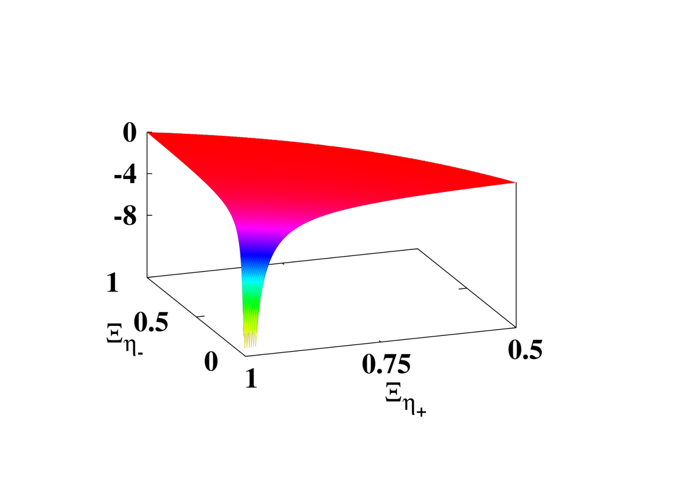
Case III: We now consider the general scenario, where the additional event efficiency, $\Xi_{\eta_{+}}$, as well as the lost event efficiency, $\Xi_{\eta_{-}}$, are both non-ideal, i.e., they both possess non-unit values. A relation involving the measured MDI-EW function, $I_{m}$, which guarantees entanglement present in a bipartite state $\rho_{AB}$, is given by

$$I_{m}(\rho_{AB})<\frac{\text{tr}(W)}{4}\left(1-\frac{1}{\Xi_{\eta_{-}}+\frac{1}{\Xi_{\eta_{+}}}-1}\right).$$

(17)

Note that the bound on $I_{m}$ reaches zero, which is the bound on MDI-EW function without any loophole in outcomes, when

$$\Xi_{\eta_{-}}+\frac{1}{\Xi_{\eta_{+}}}=2.$$

(18)

It is important to know the cases when the bound on $I_{m}$ is negative, since these instances may lead to false identifications of separable states as entangled ones. For non-negative bounds, the loophole due to lost and additional events vanishes. To visualize the bound, we plot, in Fig. 1, the upper bound on the measured MDI-EW function, $I_{m}$, for entangled Werner states with varying $\Xi_{\eta_{-}}$ and $\Xi_{\eta_{+}}$, in the non-trivial part of the region demarcated by Eq. (18).

The bound on $I_{m}$, given by the relation (17), can easily be generalized to a genuine $n$-partite MDI entanglement witness by replacing 4 with $2^{n}$ in the denominator on the RHS.

A measurement-device-independent entanglement witness had been prescribed, based on the idea of a semi-quantum game, where every entangled state yields advantage over all separable states. Here we considered the problem of detection loophole in detecting entanglement in a measurement-device-independent way. We discussed three separate cases of inefficient measurement devices, viz., the case when there are only losses in the outcomes of measurement, the case when there are only additional counts in the same, and finally the scenario where both types of the inefficiencies occur. We found that in the case of additional events, inefficiency of the measurement device cannot lead to false positives, i.e., the measurement-device-independent entanglement witness will not show any separable state as entangled. However, we showed that in the the case of lossy detectors as well as in the case when both types of inefficiencies are present, measurement-device-independent entanglement witnesses can erroneously exhibit a separable state as entangled. To avoid such misjudgments, we derived an inequality in each case, which depend on the efficiencies of the detectors involved. If a measured value of the measurement-device-independent entanglement witness satisfies the relevant inequality, for a particular set of values of the detector efficiencies, then one will reach the unambiguous conclusion of presence of entanglement in the shared quantum state under consideration. We have exemplified the results by using the Werner and noisy Greenberger-Horne-Zeilinger states.

References

- (1) R. Horodecki, P. Horodecki, M. Horodecki, and K. Horodecki, Rev. Mod. Phys. 81, 865 (2009).
- (2) O. Gühne and G. Tóth, Phys. Rep. 474, 1 (2009).
- (3) S. Das, T. Chanda, M. Lewenstein, A. Sanpera, A. Sen(De), and U. Sen, The separability versus entanglement problem, in Quantum Information: From Foundations to Quantum Technology Applications, second edition, eds. D. Bruß and G. Leuchs, Wiley, Weinheim, 2019, arXiv:1701.02187 [quant-ph].
- (4) C. H. Bennett, G. Brassard, C. Crépeau, R. Jozsa, A. Peres, and W. K. Wootters, Phys. Rev. Lett. 70, 1895 (1993).
- (5) C. H. Bennett and S. J. Wiesner, Phys. Rev. Lett. 69, 2881(1992).
- (6) A. K. Ekert, Phys. Rev. Lett. 67, 661 (1991).
- (7) A. Peres, Phys. Rev. Lett. 77, 1413 (1996).
- (8) M. Horodecki, P. Horodecki, and R. Horodecki, Phys. Lett. A. 223, 1 (1996).
- (9) P. Horodecki, Phys. Lett. A 232, 333 (1997).
- (10) J.S. Bell, Speakable and unspeakable in quantum mechanics (Cambridge University Press, New York, 1989).
- (11) B. M. Terhal, Phys. Lett. A 271, 319 (2000); D. Bruß, J. I. Cirac, P. Horodecki, F. Hulpke, B. Kraus, M. Lewenstein, and A. Sanpera, J. Mod. Opt. 49, 1399 (2002); O. Gühne and G. Tóth, Physics Reports 474, 1 (2009).
- (12) L. Di-Carlo, M. D. Reed, L. Sun, B. R. Johnson, J. M. Chow, J. M. Gambetta, L. Frunzio, S. M. Girvin, M. H. Devoret, and R. J. Schoelkopf, Nature 467, 574 (2010); N. Friis et al., Phys. Rev. X 8, 021012 (2018); A. Stute, B. Casabone, P. Schindler, T. Monz, P. O. Schmidt, B.Brandstätter, T. E. Northup and R. Blatt, Nature 485, 482 (2012); M. Cramer, A. Bernard, N. Fabbri, L. Fallani, C. Fort, S. Rosi, F. Caruso, M. Inguscio, and M. B. Plenio, Nat. Commun. 4, 2161 (2013); B. P. Lanyon, M. Zwerger, P. Jurcevic, C. Hempel, W. Dr, H. J. Briegel, R. Blatt, and C. F. Roos, Phys. Rev. Lett. 112, 100403 (2014); J. M. Chow et al., Nat. Commun. 5, 4015 (2014); C. J. Ballance et al., Nature 528, 384 (2015); X.-L. Wang et al., Phys. Rev. Lett. 117, 210502 (2016); H.-S. Zhong et al., Phys. Rev. Lett. 121, 250505 (2018); The BIG Bell Test Collaboration, Nature 557, 212 (2018).
- (13) P. Skwara, H. Kampermann, M. Kleinmann, and D. Bruß, Phys. Rev. A 76, 012312 (2007).
- (14) P. Pearle, Phys. Rev. D 2, 1418 (1970); J. F. Clauser, and M. A. Horne, Phys. Rev. D 10, 526 (1974); E. Santos, Phys. Rev. A 46, 3646 (1992); N. Gisin and B. Gisin, Phys. Lett. A 260, 323 (1999); C. Branciard, Phys. Rev. A 83, 032123 (2011); Y. Lim, M. Paternostro, J. Lee, M. Kang, and H. Jeong, Phys. Rev. A 85, 062112 (2012); K. F. Pál and T. Vértesi, Phys. Rev. A 92, 022103 (2015); J. Szangolies, H. Kampermann, and D. Bruß, Phys. Rev. Lett. 118, 260401 (2017); E. Z. Cruzeiro and N. Gisin, Phys. Rev. A 99, 022104 (2019).
- (15) C. Branciard, D. Rosset, Y. C. Liang, and N. Gisin, Phys. Rev. Lett. 110, 060405 (2013).
- (16) F. Buscemi, Phys. Rev. Lett. 108, 200401 (2012).
- (17) C. Srivastava, S. Mal, A. Sen(De), and U. Sen, arXiv:1911.02908.
- (18) M. Ansmann, H. Wang, R. C. Bialczak, M. Hofheinz, E. Lucero, M. Neeley, A. D. O’Connell, D. Sank, M. Weides, J. Wenner, A. N. Cleland, and J. M. Martinis, Nature 461, 504 (2009); J. Hofmann, M. Krug, N. Ortegel, L. Gérard, M. Weber, W.Rosenfeld, and H. Weinfurter, Science 337, 72 (2012); L. K. Shalm et al., Phys. Rev. Lett. 115, 250402 (2015); M. Giustina et al., Phys. Rev. Lett. 115, 250401 (2015); B. Hensen et al., Nature 526, 682 (2015); D. Rauch et al., Phys. Rev. Lett. 121, 080403 (2018); W. N. Plick, F. Arzani, N. Treps, E. Diamanti, and D. Markham, Phys. Rev. A 98, 062101 (2018).
- (19) K. Sen, S. Das, and U. Sen, Phys. Rev. A 100, 062333 (2019).
- (20) R. F. Werner, Phys. Rev. A 40, 4277 (1989).
- (21) D. M. Greenberger, M. A. Horne, and A. Zeilinger, in Bell’s Theorem, Quantum Theory, and Conceptions of the Universe, ed. M. Kafatos (Kluwer Academic, Dordrecht, The Netherlands, 1989); N. D. Mermin, Am. J. Phys. 58, 731 (1990).
- (22) A. Sanpera, R. Tarrach, and G. Vidal, Phys. Rev. A 58, 826 (1998).
- (23) O. Gühne and M. Seevinck, New J. Phys. 12, 053002 (2010).
- (24) G. Tóth and O. Gühne, Phys. Rev. Lett. 94, 060501 (2005).