跳到论文正文
W Papers独立论文阅读器 arXiv:2004.08950 论文正文 计算阅读时间 · 0%
引用这篇论文根据当前论文元数据生成,正式投稿前建议核对。


License: CC BY-NC-ND 4.0
arXiv:2004.08950v3 [stat.ME] 25 Nov 2021

Efficient Semiparametric Estimation of Network Treatment Effects Under Partial Interference

Chan Park    Hyunseung Kang Affiliation: [0.2cm] Department of Statistics, University of Wisconsin–Madison
Abstract

Recently, many estimators for network treatment effects have been proposed. But, their optimality properties in terms of semiparametric efficiency have yet to be resolved. We present a simple, yet flexible asymptotic framework to derive the efficient influence function and the semiparametric efficiency lower bound for a family of network causal effects under partial interference. An important corollary of our results is that one of the existing estimators by Liu et al. 2019 is locally efficient. We also present other estimators that are efficient and discuss results on adaptive estimation. We conclude by using the efficient estimators to study the direct and spillover effects of conditional cash transfer programs in Colombia.

Keywords: Direct effect, Indirect effect, Partial interference, Semiparametric efficiency

1 Introduction

1.1 Motivation: Efficient Estimators Under Partial Interference

Recently, there has been growing interest in studying causal effects under interference (Cox 1958; Rubin 1986) where the potential outcome of a study unit is affected by the treatment assignment of other study units. The most well-studied type of interference is partial interference (Sobel 2006) where study units are partitioned into non-overlapping clusters and interference only arises within units in the same cluster. Hudgens and Halloran 2008 defined various network causal effects under partial interference, notably the direct and indirect causal effects, and proposed an experimental design to estimate them. Since then, many works have proposed innovative identification and estimation strategies for various causal estimands in network settings. However, an unresolved question in this literature is determining which of the several proposed estimators is optimal in terms of semiparametric efficiency. For example, several works (Perez-Heydrich et al. 2014; Liu et al. 2016; Liu et al. 2019; Barkley et al. 2020) have examined the statistical properties of the developed estimators, but none have shown whether they achieve the semiparametric efficiency bound because the efficient influence function for the network effects has not been established yet. In contrast, without interference, it is well-established that the augmented inverse probability-weighted estimator is adaptive, locally efficient, and doubly robust for the average treatment effect; see Robins et al. 1994, Hahn 1998, Scharfstein et al. 1999a, van der Laan and Robins 2003, Hirano et al. 2003, and many other works on efficient estimation under no interference.

1.2 Our Contribution

The goal of the paper is to study optimal, semiparametric estimation of network effects under partial interference. Unfortunately, we cannot directly use traditional semiparametric theory because it assumes independent and identically distributed data (Bickel et al. 1998), which is not compatible with network data. Instead, our main contribution is to re-purpose what Bickel and Kwon 2001 calls a “nonparametric model for Markov chains” which embeds non-independent and non-identically distributed data into locally independent, linear sums so that typical semiparametric theory can be applied in a local sense; see McNeney and Wellner 2000, Bickel and Kwon 2001, Sofrygin and van der Laan 2016, and Section A.1 of the supplementary materials for additional discussions on locally linear, asymptotic embedding.

Formally, if Oi{{O}}_{i} represents all observed data from cluster i=1,…,Ni=1,\ldots,N, the approach supposes Oi{{O}}_{i} are independent of each other and each Oi{{O}}_{i} is generated from one of K<∞K<\infty densities labeled by Li=1,…,KL_{i}=1,\ldots,K, i.e.

P⁡(O1,L1,…,ON,LN)=∏i=1NP⁡(Oi,Li)\displaystyle P({{O}}_{1},L_{1},\ldots,{{O}}_{N},L_{N})=\prod_{i=1}^{N}P({{O}}_{i},L_{i}) (1a)
P⁡(Oi,Li)=∏k=1K{P⁡(Li=k)​P​(Oi∣Li=k)}𝟙​(Li=k),dim⁡(Oi)<∞,K<∞.\displaystyle P({{O}}_{i},L_{i})=\prod_{k=1}^{K}\big\{P(L_{i}=k)P({{O}}_{i}\mid L_{i}=k)\big\}^{\mathbbm{1}(L_{i}=k)},\quad{}{\rm dim}({{O}}_{i})<\infty,\quad K<\infty\ . (1b)

In words, model (1) makes the following assumptions: (a) data from each cluster ii, Oi{{O}}_{i}, are independent of each other, (b) each Oi{{O}}_{i} follows some, potentially different, nonparametric distribution labeled by cluster types LiL_{i}, and (c) the asymptotics increase the number of clusters NN while keeping the cluster size dim⁡(Oi){\rm dim}(O_{i}) bounded. Property (a) is a common assumption in partial interference (VanderWeele et al. 2014; Liu et al. 2016; Yang 2018; Liu et al. 2019; Barkley et al. 2020; Smith et al. 2020; Kilpatrick and Hudgens 2021). Property (b) is our approach to deal with Oi{{O}}_{i}’s having varying dimensions for each ii due to differences in cluster size. For example, without any covariates, if household i=1i=1 has 2 individuals, O1{{O}}_{1} is 4-dimensional. But, if household i=2i=2 has 5 individuals, O2{{O}}_{2} is 1010 dimensional, and thus the density of O1{{O}}_{1} is different from the density of O2{{O}}_{2}. Critically, it is likely that the interference pattern in a two-person household is different from that in a five-person household, and we use LiL_{i} to allow for different interference patterns; see below. For property (c), to the best of our knowledge, there is no established semiparametric theory that allows dim⁡(Oi){\rm dim}({{O}}_{i}) to grow to infinity while the elements of Oi{{O}}_{i} remain dependent arbitrarily and asymptotically, i.e. the dependence does not vanish to zero as sample size increases. Instead, (c) bounds the cluster size to allow for arbitrary dependence between units in a cluster, critically between the treatment of an individual and the outcome of his/her peer in the same cluster, and the effective sample size increases with the number of clusters NN.

As mentioned earlier, the variable LiL_{i} is a key technical device to deal with a situation where two clusters ii and i′i^{\prime} have different numbers of units, and under a nonparametric framework, two different nonparametric densities, labeled by LiL_{i}, are needed to model Oi{{O}}_{i} and Oi′{{O}}_{i^{\prime}}. An alternative to using LiL_{i} would be to assume a fixed, known, dimension-reducing model on Oi{{O}}_{i} so that clusters of varying size and critically, the dependence between units within each cluster are comparable with each other; the most popular dimension-reducing model is based on a scalar function of peers’ data (van der Laan 2014; Perez-Heydrich et al. 2014; Liu et al. 2016; Sofrygin and van der Laan 2016; Ogburn et al. 2017; Liu et al. 2019; Barkley et al. 2020). Instead, our setup allows a very general, nonparametric factorization of P⁡(Oi∣Li)P({{O}}_{i}\mid L_{i}), say P(Oi∣Li)=P(Oi​1∣Oi​2,…,Oi​dim​(Oi),Li)×⋯×P(Oi​dim​(Oi)∣Li)P({{O}}_{i}\mid L_{i})=P(O_{i1}\mid O_{i2},\ldots,O_{i{\rm dim}(O_{i})},L_{i})\times\cdots\times P(O_{i{\rm dim}(O_{i})}\mid L_{i})

Also, while (1) resembles a mixture model, the goal of the paper is not to identify or estimate unknown mixture labels LiL_{i} typical in mixture modeling. Instead, LiL_{i} is a tool to embed/approximate studies under partial interference into (1), and hence LiL_{i} is known by construction. For example, in a study on student absenteeism in Philadelphia with households as clusters, Basse and Feller 2018 proposed stratifying households by their size. Thus, a natural embedding with LiL_{i} is by household size where a household of size 2 belongs to one cluster type and a household of size 4 belongs to another cluster type. Or, in a twins study, LiL_{i} could be defined by different types or twins such as identical and fraternal twins. Section 6 contains additional discussions of model (1).

Finally, our setting differs from existing semiparametric settings under independent, but (non-)identically distributed multivariate data where the dimension of the multivariate data is often identical (Robins and Rotnitzky 1995; Rotnitzky et al. 1998; Chen et al. 2006; Vansteelandt et al. 2007). For example, in existing theoretical work on locally efficient estimators of causal effects with multivariate or repeated outcomes, it is common to make a simplifying assumption that everyone’s data have identical dimensions, say dim⁡(Oi)=T{\rm dim}({{O}}_{i})=T for all individual i=1,…,Ni=1,\ldots,N, and TT is typically defined by the number of repeated response from individual ii. Instead, the setting in the paper is closer to a conditionally independent and identically distributed setting in example 1 of Bickel and Kwon 2001 where we embed different parts of the observed data using LiL_{i} so that conditional on LiL_{i}, Oi{{O}}_{i} becomes independent and identically distributed, and we can apply the usual semiparametric theory locally in LiL_{i}.

Under model (1), we derive the globally and locally efficient influence functions and the semiparametric efficiency lower bounds for a family of network causal effects under partial interference. We remark that the target estimand is still defined as the contrasts of individual i​jij’s potential outcomes, not contrasts of cluster-level potential outcomes, and our identification, estimation, and inference strategies use individual-level observed data Oi​j{{O}}_{ij} instead of cluster-level summaries of individual-level observed data. An important corollary of our results is that the bias-corrected doubly robust estimator from Liu et al. 2019 is locally efficient for estimating the direct and indirect effects in Hudgens and Halloran 2008 and Tchetgen Tchetgen and VanderWeele 2012; in short, Liu et al. 2019’s estimator is the partial interference equivalent to the aforementioned augmented inverse probability-weighted estimator of the average treatment effect under no interference. We also present other estimators that can achieve the efficiency bound, notably a simple variant of a cross-fitting estimator (Chernozhukov et al. 2018) under partial interference that achieves the global efficiency bound. Additionally, we briefly discuss adaptive estimation, which mirrors the adaptation properties of the augmented inverse probability-weighted estimator under no interference (Scharfstein et al. 1999b). We conclude by using our efficient estimators to study the direct and spillover effects of conditional cash transfer programs on student attendance in Colombia.

2 Setup

2.1 Notation

We lay out the notations for the observed data. We denote the cluster type by Li∈{1,…,K}L_{i}\in\{1,\ldots,K\} where LiL_{i} are cluster-level variables and K<∞K<\infty is the number of cluster types. For mathematical convenience, we use cluster size to define cluster types LiL_{i} hereafter, but we emphasize that any LiL_{i} satisfying model (1) is valid for the results below. Let NN, NkN_{k}, and MkM_{k} be the number of clusters, the number of clusters from cluster type kk, and the cluster size of type kk, respectively. For each cluster i=1,…,Ni=1,\ldots,N, let Yi​j∈ℝY_{ij}\in\mathbb{R} be unit jj’s univariate outcome, Ai​j∈{0,1}A_{ij}\in\{0,1\} be unit jj’s treatment indicator where Ai​j=1A_{ij}=1 indicates unit jj is assigned to treatment and Ai​j=0A_{ij}=0 indicates unit jj is assigned to control, and Xi​j{{X}}_{ij} be unit jj’s vector of pre-treatment covariates. Let Yi=(Yi​1,…,Yi​Mk)T∈ℝMk{{Y}}_{i}=(Y_{i1},\ldots,Y_{iM_{k}})^{\mathrm{\scriptscriptstyle T}}\in\mathbb{R}^{M_{k}}, Ai=(Ai​1,…,Ai​Mk)T∈𝒜⁡(Mk){{A}}_{i}=(A_{i1},\ldots,A_{iM_{k}})^{\mathrm{\scriptscriptstyle T}}\in\mathcal{A}(M_{k}), and Xi=(Xi​1T,…,Xi​MkT)T∈𝒳⁡(k){{X}}_{i}=({{X}}_{i1}^{\mathrm{\scriptscriptstyle T}},\ldots,{{X}}_{iM_{k}}^{\mathrm{\scriptscriptstyle T}})^{\mathrm{\scriptscriptstyle T}}\in\mathcal{X}(k) be the vectorized outcome, treatment assignment, and pre-treatment covariates, respectively, for each cluster ii in cluster type kk; here, 𝒜⁡(t)\mathcal{A}(t) is a collection of tt-dimensional binary vectors and 𝒳⁡(k)\mathcal{X}(k) is the finite dimensional support of Xi{{X}}_{i} for cluster type kk. Let Oi=(Yi,Ai,Xi){{O}}_{i}=({{Y}}_{i},{{A}}_{i},{{X}}_{i}) be all the observed data from cluster ii and let LiL_{i} indicate which type cluster ii belongs to.

We use potential outcomes to define causal effects. Let Ai⁡(−j)∈𝒜⁡(Mk−1){{A}}_{{i(-j)}}\in\mathcal{A}(M_{k}-1) be the vector of treatment indicators for all units in cluster ii except unit jj. Let ai​ja_{ij}, ai{{a}}_{i}, and ai⁡(−j){{a}}_{i(-j)} be the realized values of Ai​jA_{ij}, Ai{{A}}_{i}, and Ai⁡(−j){{A}}_{{i(-j)}}, respectively. Let Yi​j​(ai)Y_{ij}({{a}}_{i}) be the potential outcome of unit jj in cluster ii under treatment vector ai{{a}}_{i} and let Yi​(ai)=(Yi​1​(ai),…,Yi​Mk​(ai))T{{Y}}_{i}({{a}}_{i})=\big(Y_{i1}({{a}}_{i}),\ldots,Y_{iM_{k}}({{a}}_{i})\big)^{\mathrm{\scriptscriptstyle T}} be the potential outcomes of all units in cluster ii. Following Hudgens and Halloran 2008 and Tchetgen Tchetgen and VanderWeele 2012, we define the unit average potential outcome for a∈{0,1}a\in\{0,1\} under a treatment allocation strategy α∈(0,1)\alpha\in(0,1) as

Y¯i​j​(a,α)=∑ai∈𝒜⁡(Mk)Yi​j​(ai)​𝟙​(ai​j=a)​π​(ai⁡(−j),α),π⁡(ai⁡(−j),α)=∏j′≠jαai​j′​(1−α)1−ai​j′.\displaystyle\overline{Y}_{ij}(a\,;\,\alpha)=\sum_{{{a}}_{i}\in\mathcal{A}(M_{k})}Y_{ij}({{a}}_{i})\mathbbm{1}(a_{ij}=a)\pi({{a}}_{{i(-j)}}\,;\,\alpha)\ ,\ \pi({{a}}_{{i(-j)}}\,;\,\alpha)=\prod_{j^{\prime}\neq j}\alpha^{a_{ij^{\prime}}}(1-\alpha)^{1-a_{ij^{\prime}}}\ .

In words, Y¯i​j​(a,α)\overline{Y}_{ij}(a\,;\,\alpha) is the average of unit i​jij’s potential outcomes when the unit’s treatment is fixed at aa and the unit’s peers in a cluster are assigned to treatment independently with probability α∈(0,1)\alpha\in(0,1). We also define the cluster average potential outcome as Y¯i​(a,α)=Mk−1​∑j=1MkY¯i​j​(a,α)\overline{Y}_{i}(a\,;\,\alpha)=M_{k}^{-1}\sum_{j=1}^{M_{k}}\overline{Y}_{ij}(a\,;\,\alpha).

Finally, for a vector VNV_{N}, let VN=OP​(1)V_{N}=O_{P}(1) and VN=oP​(1)V_{N}=o_{P}(1) be the usual big-O and little-O notations, respectively. Let ∥⋅∥2\|\cdot\|_{2} be the 2-norm of a vector and a matrix. Let V⊧WV\rotatebox[origin]{90.0}{$\models$}\,W denote independence between two random variables VV and WW.

2.2 Family of Causal Estimands Under Partial Interference

Consider the set of causal estimands in cluster type kk, denoted by Θk\Theta_{k}, and the set of causal estimands across all clusters, denoted by T\mathrm{T}:

Θk={θk∈ℝ|\displaystyle\hskip 0.0pt\Theta_{k}=\Big\{{\theta}_{k}\in\mathbb{R}\,\Big|\, θk=θk​(αk,αk′)=∑ai∈𝒜⁡(Mk)E⁡{wkT​(ai,Xi,αk,αk′)​Yi​(ai)∣Li=k},\displaystyle{\theta}_{k}={\theta}_{k}(\alpha_{k},\alpha_{k}^{\prime})=\sum_{{{a}}_{i}\in\mathcal{A}(M_{k})}{E}\big\{{{w}}_{k}^{\mathrm{\scriptscriptstyle T}}({{a}}_{i},{{X}}_{i}\,;\,\alpha_{k},\alpha_{k}^{\prime}){{Y}}_{i}({{a}}_{i})\mid L_{i}=k\big\},
αk,αk′∈(0,1),wk(ai,xi;αk,αk′)∈ℝMk,∥wk(ai,xi;αk,αk′)∥2<∞},\displaystyle\alpha_{k},\alpha_{k}^{\prime}\in(0,1),\ {{w}}_{k}({{a}}_{i},{{x}}_{i}\,;\,\alpha_{k},\alpha_{k}^{\prime})\in\mathbb{R}^{M_{k}},\big\|{{w}}_{k}({{a}}_{i},{{x}}_{i}\,;\,\alpha_{k},\alpha_{k}^{\prime})\big\|_{2}<\infty\ \Big\}\ ,
T={τ∈ℝ|\displaystyle\hskip-28.45274pt\mathrm{T}=\Big\{{\tau}\in\mathbb{R}\,\Big|\, τ=vT​(p)​θ,v⁡(p)=(v1​(p1),…,vK​(pK))T,θ=(θ1,…,θK)T,\displaystyle{\tau}={{v}}^{\mathrm{\scriptscriptstyle T}}({{p}}){\theta},\ {{v}}({{p}})=\big(v_{1}(p_{1}),\ldots,v_{K}(p_{K})\big)^{\mathrm{\scriptscriptstyle T}},\ {\theta}=({\theta}_{1},\ldots,{\theta}_{K})^{\mathrm{\scriptscriptstyle T}},
vk(⋅) is continuously differentiable,pk=pr(Li=k),θk∈Θk}.\displaystyle\ v_{k}(\cdot)\text{ is continuously differentiable},\ p_{k}={\rm pr}(L_{i}=k),\ {\theta}_{k}\in\Theta_{k}\Big\}\ .

In words, for each cluster type kk, the set Θk\Theta_{k} consists of parameters θk​(αk,αk′)\theta_{k}(\alpha_{k},\alpha_{k}^{\prime}), which are linear, weighted sums of expectation of potential outcomes in cluster ii. The weights wk​(ai,Xi,αk,αk′){{w}}_{k}({{a}}_{i},{{X}}_{i}\,;\,\alpha_{k},\alpha_{k}^{\prime}) are determined by the causal estimand of interest and the sum is over all possible values of the treatment vector ai∈𝒜⁡(Mk){{a}}_{i}\in\mathcal{A}(M_{k}). Second, the set T{\rm T} consists of estimands τ\tau, which are weighted sums of θk​(αk,αk′)\theta_{k}(\alpha_{k},\alpha_{k}^{\prime}) with weights vk​(pk)v_{k}(p_{k}). The weights vk​(⋅)v_{k}(\cdot) are also determined by the causal estimand of interest.

At a high level, both sets Θk\Theta_{k} and T{\rm T} are abstractions of familiar causal parameters under partial interference. For example, suppose the target estimand is the direct effect τDE​(α)=E⁡{Y¯i​(1,α)−Y¯i​(0,α)}{\tau}^{\rm DE}(\alpha)={E}\big\{\overline{Y}_{i}(1\,;\,\alpha)-\overline{Y}_{i}(0\,;\,\alpha)\big\}, which is counterpart of the direct effect defined in Hudgens and Halloran 2008 under an infinite population framework. If we choose the weights wk{{w}}_{k} and vkv_{k} as

wk​(ai,α)=1Mk​[{𝟙​(ai​1=1)−𝟙​(ai​1=0)}​π​(ai⁡(−1),α){𝟙​(ai​j=1)−𝟙​(ai​j=0)}​π​(ai⁡(−j),α){𝟙​(ai​Mk=1)−𝟙​(ai​Mk=0)}​π​(ai⁡(−Mk),α)],vk​(pk)=pk=P⁡(Li=k),\displaystyle\hskip-2.84544pt{{w}}_{k}({{a}}_{i}\,;\,\alpha)=\frac{1}{M_{k}}\begin{bmatrix}\big\{\mathbbm{1}\big(a_{i1}=1)-\mathbbm{1}\big(a_{i1}=0)\big\}\pi({{a}}_{i(-1)}\,;\,\alpha)\\[-2.84544pt] \vdots\\[-2.84544pt] \big\{\mathbbm{1}\big(a_{ij}=1)-\mathbbm{1}\big(a_{ij}=0)\big\}\pi({{a}}_{i(-j)}\,;\,\alpha)\\[-2.84544pt] \vdots\\[-2.84544pt] \big\{\mathbbm{1}\big(a_{iM_{k}}=1)-\mathbbm{1}\big(a_{iM_{k}}=0)\big\}\pi({{a}}_{i(-M_{k})}\,;\,\alpha)\end{bmatrix}\,,\,v_{k}(p_{k})=p_{k}=P(L_{i}=k)\,,\hskip-2.84544pt (2)

this leads θk=θkDE​(α)=E⁡{Y¯i​(1,α)−Y¯i​(0,α)∣Li=k}∈Θk\theta_{k}={\theta}_{k}^{\rm DE}(\alpha)={E}\big\{\overline{Y}_{i}(1\,;\,\alpha)-\overline{Y}_{i}(0\,;\,\alpha)\mid L_{i}=k\big\}\in\Theta_{k}, the direct effect in cluster type kk, and τ=τDE​(α)=E⁡{Y¯i​(1,α)−Y¯i​(0,α)}∈T\tau={\tau}^{\rm DE}(\alpha)={E}\big\{\overline{Y}_{i}(1\,;\,\alpha)-\overline{Y}_{i}(0\,;\,\alpha)\big\}\in\mathrm{T}. Similarly, by taking each entry of the weights wkw_{k} as 𝟙​(ai​j=0)​{π⁡(ai⁡(−j),α)−π⁡(ai⁡(−j),α′)}/Mk\mathbbm{1}(a_{ij}=0)\{\pi({{a}}_{i(-j)}\,;\,\alpha)-\pi({{a}}_{i(-j)}\,;\,\alpha^{\prime})\}/M_{k}, we arrive at θk=θkIE​(α,α′)=E⁡{Y¯i​(0,α)−Y¯i​(0,α′)∣Li=k}∈Θk{\theta}_{k}={\theta}_{k}^{\rm IE}(\alpha,\alpha^{\prime})={E}\big\{\overline{Y}_{i}(0\,;\,\alpha)-\overline{Y}_{i}(0\,;\,\alpha^{\prime})\mid L_{i}=k\big\}\in\Theta_{k}, the indirect effect in cluster type kk, and τ=τIE​(α,α′)=E⁡{Y¯i​(0,α)−Y¯i​(0,α′)}∈T{\tau}={\tau}^{\rm IE}(\alpha,\alpha^{\prime})={E}\big\{\overline{Y}_{i}(0\,;\,\alpha)-\overline{Y}_{i}(0\,;\,\alpha^{\prime})\big\}\in\mathrm{T}, the indirect effect. Section A.2 of the supplementary material shows that under certain growth conditions, existing finite sample causal effects in partial interference, say total effects, overall effects, or spillover effects among subgroups, can be asymptotically embedded into Θk\Theta_{k} and T\mathrm{T}.

To identify the causal estimands in T\mathrm{T}, let g⁡(a,x,k)=E⁡(Yi∣Ai=a,Xi=x,Li=k){{g}}({{a}},{{x}},k)={E}({{Y}}_{i}\mid{{A}}_{i}={{a}},{{X}}_{i}={{x}},L_{i}=k) be the vector of conditional expected outcomes in cluster ii and Σ⁡(a,x,k)=var⁡(Yi∣Ai=a,Xi=x,Li=k)\Sigma({{a}},{{x}},k)={\rm var}({{Y}}_{i}\mid{{A}}_{i}={{a}},{{X}}_{i}={{x}},L_{i}=k) be its conditional covariance. The outcome model g⁡(a,x,k){{g}}({{a}},{{x}},k) is a generalization of the usual outcome model to partial interference settings where now, the outcomes in a cluster are jointly modeled. Also, let e⁡(a∣x,k)=pr⁡(Ai=a∣Xi=x,Li=k)e({{a}}\mid{{x}},k)={\rm pr}({{A}}_{i}={{a}}\mid{{X}}_{i}={{x}},L_{i}=k) be the probability of observing treatment vector a∈𝒜⁡(Mk){{a}}\in\mathcal{A}(M_{k}) given covariates x{{x}} in cluster type kk. The propensity score model e⁡(a∣x,k)e({{a}}\mid{{x}},k) is a generalization of the propensity score (Rosenbaum and Rubin 1983) to partial interference settings where all treatment assignments in a cluster are jointly modeled. Assumption 2.1 lays out the identifying assumptions for a parameter in T\mathrm{T}; see Liu et al. 2019 for similar conditions.

Assumption 2.1.

For all a∈𝒜⁡(Mk){{a}}\in\mathcal{A}(M_{k}), x∈𝒳⁡(k){{x}}\in\mathcal{X}(k), and k=1,…,Kk=1,\ldots,K, we have the following conditions: (A1) Consistency: Yi=∑k=1K𝟙​(Li=k)​∑ai∈𝒜⁡(Mk)𝟙​(Ai=ai)​Yi​(ai){{Y}}_{i}=\sum_{k=1}^{K}\mathbbm{1}(L_{i}=k)\sum_{{{a}}_{i}\in\mathcal{A}(M_{k})}\mathbbm{1}({{A}}_{i}={{a}}_{i}){{Y}}_{i}({{a}}_{i}); (A2) Conditional Ignorability: Yi​(a)⊧Ai|(Xi=x,Li=k){{Y}}_{i}({{a}})\rotatebox[origin]{90.0}{$\models$}\,{{A}}_{i}\mid({{X}}_{i}={{x}},L_{i}=k); (A3) Positivity/Overlap: There exists a positive constant cc so that c<e⁡(a∣x,k)<1−cc<e({{a}}\mid{{x}},k)<1-c; (A4) Moments: E⁡{g⁡(a,Xi,k)∣Li=k}{E}\big\{{{g}}({{a}},{{X}}_{i},k)\mid L_{i}=k\big\} and E⁡{Σ⁡(a,Xi,k)∣Li=k}{E}\big\{\Sigma({{a}},{{X}}_{i},k)\mid L_{i}=k\big\} exist and are finite. Also, Σ⁡(a,x,k)\Sigma({{a}},{{x}},k) is positive definite.

Conditions (A1)–(A3) are natural extensions of consistency, conditional ignorability and overlap to partial interference settings; see Imbens and Rubin 2015 and Hernán and Robins 2020 for textbook discussions. Condition (A4) ensures that the expectations and covariances are well-defined. Under Assumption 2.1, a causal estimand τ∈T{\tau}\in\mathrm{T} can be identified from (Oi,Li)({{O}}_{i},L_{i}) as

τ=vT​(p)​θ=∑k=1Kvk​(pk)​[∑ai∈𝒜⁡(Mk)E⁡{wkT​(ai,Xi)​g​(ai,Xi,k)∣Li=k}].\displaystyle{\tau}={{v}}^{\mathrm{\scriptscriptstyle T}}({{p}}){\theta}=\sum_{k=1}^{K}v_{k}(p_{k})\bigg[\sum_{{{a}}_{i}\in\mathcal{A}(M_{k})}{E}\big\{{{w}}_{k}^{\mathrm{\scriptscriptstyle T}}({{a}}_{i},{{X}}_{i}){{g}}({{a}}_{i},{{X}}_{i},k)\mid L_{i}=k\big\}\bigg]\ . (3)

Here, wk​(ai,Xi){{w}}_{k}({{a}}_{i},{{X}}_{i}) is shorthand for wk​(ai,Xi,αk,αk′){{w}}_{k}({{a}}_{i},{{X}}_{i}\,;\,\alpha_{k},\alpha_{k}^{\prime}). The rest of the paper will focus on efficient estimation of the functional based on the observed data in (3) under model (1).

3 Semiparametric Efficiency Under Partial Interference

3.1 Global Efficiency

Let p∗{{p}}^{*}, θ∗{\theta}^{*}, τ∗{\tau}^{*}, e∗e^{*}, g∗{{g}}^{*}, and Σ∗\Sigma^{*} denote the true values of p{{p}}, θ{\theta}, τ{\tau}, ee, g{{g}}, and Σ\Sigma, respectively. Theorem 3.1 presents our first main result where we derive the globally efficient influence function and the semiparametric efficiency bound of τ∗∈T{\tau}^{*}\in\mathrm{T} in model ℳNP={PO,L=P⁡(O1,L1,…,ON,LN)|P⁡(⋅)​ satisfies (1)}\mathcal{M}_{{\rm NP}}=\big\{P_{{{O}},L}=P({{{O}}_{1},L_{1},\ldots,{{O}}_{N},L_{N}})\,\big|\,P(\cdot)\text{ satisfies \eqref{eq:NPmodel}}\big\}.

Theorem 3.1 (Global Efficiency).

Let τ∗∈T{\tau}^{*}\in\mathrm{T} be the parameter defined in (3) and suppose Assumption 2.1 holds. If pk∗p_{k}^{*}s are unknown, the efficient influence function of τ∗{\tau}^{*} under model ℳNP\mathcal{M}_{{\rm NP}} is

φ⁡(τ∗)\displaystyle\varphi({\tau}^{*}) =∑k=1Kvk​(pk∗)​φk​(θk∗)+∑k=1K{𝟙​(Li=k)−pk∗}​∂vk​(pk∗)∂pk​θk∗\displaystyle=\sum_{k=1}^{K}v_{k}(p_{k}^{*})\varphi_{k}({\theta}_{k}^{*})+\sum_{k=1}^{K}\Big\{\mathbbm{1}(L_{i}=k)-p_{k}^{*}\Big\}\frac{\partial v_{k}(p_{k}^{*})}{\partial p_{k}}{\theta}_{k}^{*}

where φk​(θk∗)=𝟙​(Li=k)​{ϕk​(Oi,e∗,g∗)−θk∗}/pk∗\varphi_{k}({\theta}_{k}^{*})=\mathbbm{1}(L_{i}=k)\big\{\phi_{k}({{O}}_{i},e^{*},{{g}}^{*})-{\theta}_{k}^{*}\big\}/p_{k}^{*} with

ϕk​(Oi,e∗,g∗)=𝟙​(Li=k)​[wkT​(Ai,Xi)​{Yi−g∗​(Ai,Xi,k)}e∗​(Ai∣Xi,k)+∑ai∈𝒜⁡(Mk)wkT​(ai,Xi)​g∗​(ai,Xi,k)].\displaystyle\hskip-5.69046pt\phi_{k}({{O}}_{i},e^{*},{{g}}^{*})=\mathbbm{1}\big(L_{i}=k\big)\bigg[\frac{{{w}}_{k}^{\mathrm{\scriptscriptstyle T}}({{A}}_{i},{{X}}_{i})\big\{{{Y}}_{i}-{{g}}^{*}({{A}}_{i},{{X}}_{i},k)\big\}}{e^{*}({{A}}_{i}\mid{{X}}_{i},k)}+\hskip-8.5359pt\sum_{{{a}}_{i}\in\mathcal{A}(M_{k})}\hskip-8.5359pt{{w}}_{k}^{\mathrm{\scriptscriptstyle T}}({{a}}_{i},{{X}}_{i}){{g}}^{*}({{a}}_{i},{{X}}_{i},k)\bigg]\ . (4)

Moreover, the semiparametric efficiency bound of τ∗{\tau}^{*} in model ℳNP\mathcal{M}_{{\rm NP}} is var​{φ⁡(τ∗)}{\rm var}\big\{\varphi({\tau}^{*})\big\}.

See the supplementary materials for the result when pk∗p_{k}^{*}s are known. We make some remarks about Theorem 3.1. First, if K=1K=1 and Mk=1M_{k}=1, our result would reduce to Theorem 1 in Hahn 1998. Second, some of the usual components from the efficient influence function of the average treatment effect without interference are still present in equation (4), most notably the residual-weighting term by the propensity score, i.e. {Yi−g∗​(Ai,Xi,k)}/e∗​(Ai∣Xi,k)\big\{{{Y}}_{i}-{{g}}^{*}({{A}}_{i},{{X}}_{i},k)\big\}/e^{*}({{A}}_{i}\mid{{X}}_{i},k), and the outcome regression term, i.e. ∑ai∈𝒜⁡(Mk)wkT​(ai,Xi)​g∗​(ai,Xi,k)−θk∗\sum_{{{a}}_{i}\in\mathcal{A}(M_{k})}{{w}}_{k}^{\mathrm{\scriptscriptstyle T}}({{a}}_{i},{{X}}_{i}){{g}}^{*}({{a}}_{i},{{X}}_{i},k)-{\theta}_{k}^{*}. However, there are new terms to account for under dependence between units, specifically (i) a weighing term wk{{w}}_{k} that weighs peers’ influence on one’s own outcome, (ii) a non-diagonal covariance matrix Σ∗\Sigma^{*}, (iii) a multivariate outcome regression, which leads to multivariate residuals, and (iv) a propensity score that depends on a vector of treatment assignments instead of one’s own treatment assignment. Third, in Section A.3 of the supplementary materials, we discuss the efficient influence function in (4) can be used to construct a doubly robust estimator, resolving a conjecture discussed in Section 7 of Liu et al. 2019 about the property of doubly robust estimators under partial interference.

3.2 Local Efficiency

Often in practice, investigators posit parametric or semiparametric models to estimate the outcome model g{{g}} or the propensity score model ee (Perez-Heydrich et al. 2014; Liu et al. 2016; Liu et al. 2019; Barkley et al. 2020). To this end, this section presents our second main result where we derive locally efficient semiparametric estimators for parameters in T\mathrm{T}. To begin, we define model spaces ℳg⊆ℳNP\mathcal{M}_{g}\subseteq\mathcal{M}_{{\rm NP}} and ℳe⊆ℳNP\mathcal{M}_{e}\subseteq\mathcal{M}_{{\rm NP}} that restrict the outcome and propensity score models to those specified by the investigator; i.e.

ℳg={PO,L∈ℳNP|\displaystyle\mathcal{M}_{g}=\big\{P_{{{O}},L}\in\mathcal{M}_{{\rm NP}}\,\big|\, there is a unique βg∗ such that g∗(a,x,k)=g(a,x,k;βg∗)},\displaystyle\text{there is a unique }{\beta}_{g}^{*}\text{ such that }{{g}}^{*}({{a}},{{x}},k)={{g}}({{a}},{{x}},k\,;\,{\beta}_{g}^{*})\big\}\ ,
ℳe={PO,L∈ℳNP|\displaystyle\mathcal{M}_{e}=\big\{P_{{{O}},L}\in\mathcal{M}_{{\rm NP}}\,\big|\, there is a unique βe∗ such that e∗(a∣x,k)=e(a∣x,k;βe∗)}.\displaystyle\text{there is a unique }{\beta}_{e}^{*}\text{ such that }e^{*}({{a}}\mid{{x}},k)=e({{a}}\mid{{x}},k\,;\,{\beta}_{e}^{*})\big\}\ .

Some commonly used models for ℳg\mathcal{M}_{g} and ℳe\mathcal{M}_{e} include generalized mixed effects models, score equations, quasi-likelihoods, or generalized estimating equations.

The outcome regression model ℳg\mathcal{M}_{g} can encode information about a known exposure mapping. For example, consider a two-person household where individual 1’s outcome depends on individual 2’s treatment status, but individual 2’s outcome does not depend on individual 1’s treatment status. In short, there is asymmetric interference where there is no interference from individual 1 to individual 2, but there is interference from individual 2 to individual 1. Also, practically speaking, this type of asymmetric interference may be plausible in some vaccine studies where, depending on the vaccine, vaccinated individuals’ outcomes are unlikely to be affected by their peers’ vaccination status, i.e. treatment, but the unvaccinated individuals’ outcomes may be affected by their peers’ vaccination status. Then, one way to encode this exposure map is through a simple linear model for g=(g1,g2)T{{g}}=(g_{1},g_{2})^{\mathrm{\scriptscriptstyle T}}, i.e.

g⁡(Ai,Xi,k,βg)=[g1​(Ai,Xi,k,βg)g2​(Ai,Xi,k,βg)]=[βg​10+βg​11​Ai​1+βg​12​Ai​2+βg​13T​Xi​1+βg​14T​Xi​2βg​20+βg​21​Ai​2+βg​22T​Xi​1+βg​23T​Xi​2].\displaystyle{{g}}({{A}}_{i},{{X}}_{i},k\,;\,\beta_{g})=\begin{bmatrix}g_{1}({{A}}_{i},{{X}}_{i},k\,;\,\beta_{g})\\ g_{2}({{A}}_{i},{{X}}_{i},k\,;\,\beta_{g})\end{bmatrix}=\begin{bmatrix}\beta_{g10}+\beta_{g11}A_{i1}+\beta_{g12}A_{i2}+\beta_{g13}^{\mathrm{\scriptscriptstyle T}}{{X}}_{i1}+\beta_{g14}^{\mathrm{\scriptscriptstyle T}}{{X}}_{i2}\\ \beta_{g20}+\beta_{g21}A_{i2}+\beta_{g22}^{\mathrm{\scriptscriptstyle T}}{{X}}_{i1}+\beta_{g23}^{\mathrm{\scriptscriptstyle T}}{{X}}_{i2}\end{bmatrix}\ .

As another example, consider the setting by Sofrygin and van der Laan 2016 and Ogburn et al. 2017 where the exposure mapping is restricted to a map where (i) the individual-level outcome regression gj​(Ai,Xi,Li)g_{j}({{A}}_{i},{{X}}_{i},L_{i}) is identical across jj, i.e. symmetric interference, and (ii) the dependence on (Ai⁡(−j),Xi⁡(−j))({{A}}_{i(-j)},{{X}}_{i(-j)}) occurs only through finite, fixed dimensional summary statistics, say (Ai⁡(−j)s,Xi⁡(−j)s)({{A}}_{i(-j)}^{s},{{X}}_{i(-j)}^{s}). Then, one way to encode this type of exposure map is through a linear model for g=(g1,…,gMk)T{{g}}=(g_{1},\ldots,g_{M_{k}})^{\mathrm{\scriptscriptstyle T}}, i.e.

g⁡(Ai,Xi,k,βg)=[g1​(Ai,Xi,k,βg)gMk​(Ai,Xi,k,βg)],gj​(Ai,Xi,k,βg)=βg​0+βg​1T​[Ai​jAi⁡(−j)s]+βg​2T​[Xi​jXi⁡(−j)s].\displaystyle{{g}}({{A}}_{i},{{X}}_{i},k\,;\,\beta_{g})=\begin{bmatrix}g_{1}({{A}}_{i},{{X}}_{i},k\,;\,\beta_{g})\\[-2.84544pt] \vdots\\ g_{M_{k}}({{A}}_{i},{{X}}_{i},k\,;\,\beta_{g})\end{bmatrix}\ ,\ g_{j}({{A}}_{i},{{X}}_{i},k\,;\,\beta_{g})=\beta_{g0}+\beta_{g1}^{\mathrm{\scriptscriptstyle T}}\begin{bmatrix}A_{ij}\\ {{A}}_{i(-j)}^{s}\end{bmatrix}+\beta_{g2}^{\mathrm{\scriptscriptstyle T}}\begin{bmatrix}{{X}}_{ij}\\ {{X}}_{i(-j)}^{s}\end{bmatrix}\ .

Let β^=(β^eT,β^gT)T\widehat{{\beta}}=\big(\widehat{{\beta}}_{e}^{\mathrm{\scriptscriptstyle T}},\widehat{{\beta}}_{g}^{\mathrm{\scriptscriptstyle T}}\big)^{\mathrm{\scriptscriptstyle T}} be an estimate of β∗=(βe∗,T,βg∗,T)T{\beta}^{*}=({\beta}_{e}^{*,\mathrm{\scriptscriptstyle T}},{\beta}_{g}^{*,\mathrm{\scriptscriptstyle T}})^{\mathrm{\scriptscriptstyle T}} in ℳg\mathcal{M}_{g} and ℳe\mathcal{M}_{e}. For τ∗∈T{\tau}^{*}\in\mathrm{T}, let τ^=vT​(p^)​θ^\widehat{{\tau}}={{v}}^{\mathrm{\scriptscriptstyle T}}(\widehat{{{p}}})\widehat{{\theta}} be the estimator of τ∗{\tau}^{*} where p^=(p^1,…,p^K)T\widehat{{{p}}}=(\widehat{p}_{1},\ldots,\widehat{p}_{K})^{\mathrm{\scriptscriptstyle T}}, p^k=Nk/N\widehat{p}_{k}=N_{k}/N, and θ^\widehat{{\theta}} is the solution to the equation 0=∑i=1NΨθ​(θ^,β^)0=\sum_{i=1}^{N}\Psi_{\theta}(\widehat{{\theta}},\widehat{{\beta}}). Here, Ψθ​(θ,β^)=(Ψθ,1​(θ1,β^),…,Ψθ,K​(θK,β^))T\Psi_{\theta}({\theta},\widehat{{\beta}})=\big(\Psi_{{\theta},1}({\theta}_{1},\widehat{{\beta}}),\ldots,\Psi_{{\theta},K}({\theta}_{K},\widehat{{\beta}})\big)^{\mathrm{\scriptscriptstyle T}} and Ψθ,k​(θk,β^)=𝟙​(Li=k)​{ϕk​(Oi,e⁡(⋅,β^e),g⁡(⋅,β^g))−θk}\Psi_{{\theta},k}({\theta}_{k},\widehat{{\beta}})=\mathbbm{1}(L_{i}=k)\big\{\phi_{k}\big({{O}}_{i},e(\cdot\,;\,\widehat{{\beta}}_{e}),{{g}}(\cdot\,;\,\widehat{{\beta}}_{g})\big)-{\theta}_{k}\big\} where ϕk​(Oi,e⁡(⋅,β^e),g⁡(⋅,β^g))\phi_{k}\big({{O}}_{i},e(\cdot\,;\,\widehat{{\beta}}_{e}),{{g}}(\cdot\,;\,\widehat{{\beta}}_{g})\big) is obtained by plugging in parametrically estimated ee and g{{g}} in (4), i.e.

ϕk​(Oi,e⁡(⋅,β^e),g⁡(⋅,β^g))\displaystyle\phi_{k}\big({{O}}_{i},e(\cdot\,;\,\widehat{{\beta}}_{e}),{{g}}(\cdot\,;\,\widehat{{\beta}}_{g})\big)
=𝟙​(Li=k)​[wkT​(Ai,Xi)​{Yi−g⁡(Ai,Xi,k,β^g)}e⁡(Ai∣Xi,k;β^e)+∑ai∈𝒜⁡(Mk)wkT​(ai,Xi)​g​(ai,Xi,k,β^g)].\displaystyle=\mathbbm{1}(L_{i}=k)\bigg[\frac{{{w}}_{k}^{\mathrm{\scriptscriptstyle T}}({{A}}_{i},{{X}}_{i})\big\{{{Y}}_{i}-{{g}}({{A}}_{i},{{X}}_{i},k\,;\,\widehat{{\beta}}_{g})\big\}}{e({{A}}_{i}\mid{{X}}_{i},k\,;\,\widehat{{\beta}}_{e})}+\hskip-8.5359pt\sum_{{{a}}_{i}\in\mathcal{A}(M_{k})}\hskip-8.5359pt{{w}}_{k}^{\mathrm{\scriptscriptstyle T}}({{a}}_{i},{{X}}_{i}){{g}}({{a}}_{i},{{X}}_{i},k\,;\,\widehat{{\beta}}_{g})\bigg]\ .

Theorem 3.2 presents asymptotic properties of τ^\widehat{{\tau}} under mild regularity conditions on the estimated model parameters β^\widehat{{\beta}}; these are typical for semiparametric estimators of the propensity score or the outcome model (van der Vaart 1998).

Theorem 3.2 (Local Efficiency).

Suppose Assumption 2.1 and conditions (R1)–(R4) in the supplementary material hold. Let β†{\beta}^{\dagger} be the probability limit of β^\widehat{{\beta}}. Then, under model ℳe∪ℳg\mathcal{M}_{e}\cup\mathcal{M}_{g}, we have N1/2(τ^−τ∗)=N−1/2∑i=1Nφ(τ∗,β†)+oP(1)N^{1/2}\big(\widehat{{\tau}}-{\tau}^{*}\big)=N^{-1/2}\sum_{i=1}^{N}\varphi({\tau}^{*},{\beta}^{\dagger})+o_{P}(1) where

φ⁡(τ∗,β†)\displaystyle\varphi({\tau}^{*},{\beta}^{\dagger}) =∑k=1K[vk​(pk∗)​φk​(θk∗,β†)+{𝟙​(Li=k)−pk∗}​∂vk​(pk∗)∂pk​θk∗].\displaystyle=\sum_{k=1}^{K}\bigg[v_{k}(p_{k}^{*})\varphi_{k}({\theta}_{k}^{*},{\beta}^{\dagger})+\Big\{\mathbbm{1}(L_{i}=k)-p_{k}^{*}\Big\}\frac{\partial v_{k}(p_{k}^{*})}{\partial p_{k}}{\theta}_{k}^{*}\bigg]\ .

Here, φk​(θk∗,β†)=𝟙​(Li=k)​{ϕk​(Oi,e⁡(⋅,βe†),g⁡(⋅,βg†))−θk∗}/pk∗\varphi_{k}({\theta}_{k}^{*},{\beta}^{\dagger})=\mathbbm{1}(L_{i}=k)\big\{\phi_{k}\big({{O}}_{i},e(\cdot\,;\,{\beta}_{e}^{\dagger}),{{g}}(\cdot\,;\,{\beta}_{g}^{\dagger})\big)-{\theta}_{k}^{*}\big\}/p_{k}^{*} where ϕk​(Oi,e⁡(⋅,βe†),g⁡(⋅,βg†))\phi_{k}\big({{O}}_{i},e(\cdot\,;\,{\beta}_{e}^{\dagger}),{{g}}(\cdot\,;\,{\beta}_{g}^{\dagger})\big) is obtained from equation (4) by plugging in e⁡(⋅,βe†)∈ℳee(\cdot\,;\,{\beta}_{e}^{\dagger})\in\mathcal{M}_{e} and g⁡(⋅,βg†)∈ℳg{{g}}(\cdot\,;\,{\beta}_{g}^{\dagger})\in\mathcal{M}_{g}. Also, τ^\widehat{{\tau}} is locally efficient under ℳe∩ℳg\mathcal{M}_{e}\cap\mathcal{M}_{g}.

Theorem 3.2 states that τ^\widehat{{\tau}} is a consistent estimator of τ∗{\tau}^{*} so long as either the propensity score or the outcome regression is correctly modeled by the investigator. For example, consider the following efficient estimators for the direct and indirect effects:

τ^DE(α)=1N∑k=1K∑i:Li=k{ψ^k(1,α)−ψ^k(0,α)},τ^IE(α,α′)=1N∑k=1K∑i:Li=k{ψ^k(0,α)−ψ^k(0,α′)}\displaystyle\hskip-2.84544pt\widehat{{\tau}}^{{\rm DE}}(\alpha)\hskip-1.42271pt=\hskip-1.42271pt\frac{1}{N}\sum_{k=1}^{K}\sum_{i:L_{i}=k}\hskip-2.84544pt\big\{\widehat{\psi}_{k}(1,\alpha)-\widehat{\psi}_{k}(0,\alpha)\big\}\ ,\ \widehat{{\tau}}^{{\rm IE}}(\alpha,\alpha^{\prime})\hskip-1.42271pt=\hskip-1.42271pt\frac{1}{N}\sum_{k=1}^{K}\sum_{i:L_{i}=k}\hskip-2.84544pt\big\{\widehat{\psi}_{k}(0,\alpha)-\widehat{\psi}_{k}(0,\alpha^{\prime})\big\} (5)

where

ψ^k​(a,α)=1Mk​∑j=1Mk∑ai∈𝒜⁡(Mk)s.t.ai​j=a[𝟙​(Ai=ai)​{Yi​j−gj​(ai,Xi,k,β^g)}e⁡(ai∣Xi,k;β^e)+gj​(ai,Xi,k,β^g)]​π​(ai⁡(−j),α).\displaystyle\widehat{\psi}_{k}(a,\alpha)=\frac{1}{M_{k}}\sum_{j=1}^{M_{k}}\sum_{\begin{subarray}{c}{{a}}_{i}\in\mathcal{A}(M_{k})\\ {\rm s.t.}a_{ij}=a\end{subarray}}\Bigg[\frac{\mathbbm{1}({{A}}_{i}={{a}}_{i})\big\{Y_{ij}-g_{j}({{a}}_{i},{{X}}_{i},k\,;\,\widehat{{\beta}}_{g})\big\}}{e({{a}}_{i}\mid{{X}}_{i},k\,;\,\widehat{{\beta}}_{e})}+g_{j}({{a}}_{i},{{X}}_{i},k\,;\,\widehat{{\beta}}_{g})\Bigg]\pi({{a}}_{i(-j)}\,;\,\alpha)\ .

Here, gjg_{j} is jjth component of g{{g}}, i.e. the outcome regression of individual jj. If the propensity score e∗e^{*} is known, say because the data was generated from a network randomized experiment (Hudgens and Halloran 2008), the estimators in (5) will be consistent. If, in addition, the outcome regression g∗g^{*} is correctly specified, the estimators will be locally efficient. Critically, the existing bias-corrected doubly robust estimator of Liu et al. 2019 for the direct and indirect effects is asymptotically equivalent to (5) and hence efficient; this resolves a long-standing question on optimal semiparametric estimation direct and spillover effects under partial interference.

Corollary 3.1 (Efficiency of the Estimator of Liu et al. 2019).

Suppose that (i) estimators of gg and ee in Section 3.2 are the same as those used in Liu et al. 2019 and (ii) both the propensity score and the outcome model are correctly specified, i.e. ℳe∩ℳg\mathcal{M}_{e}\cap\mathcal{M}_{g}. Then, the bias-corrected doubly robust estimator of Liu et al. 2019 is locally efficient under ℳe∩ℳg\mathcal{M}_{e}\cap\mathcal{M}_{g}.

We remark that our results can also be used to derive efficient estimators of overall and total effects in Liu et al. 2019. Also, Section A.4 of the supplementary material numerically illustrates Theorem 3.2. Broadly speaking, Theorem 3.2 and the bias-corrected estimator of Liu et al. 2019 can be seen as the partial interference analog of the well-known result on the efficiency and double-robustness of the augmented inverse probability-weighted estimator under no interference (Robins et al. 1994; Scharfstein et al. 1999a).

We end the section by briefly summarizing two properties related to adaptive estimation under partial interference; see Section A.5 of the supplementary material for details. First, the doubly robust estimators in Theorem 3.2 can still achieve the best possible variance regardless of the knowledge of the propensity score. Second, if the investigator uses estimators that account for interference, but the true data generating model has no interference, the doubly robust estimators in Theorem 3.2 are consistent, but generally inefficient. In other words, the estimators do not adapt to the knowledge about exposure mappings. This suggests that potential side-information about exposure mappings may play a critical role, both in terms of consistency and efficiency of estimators. Also, these adaptation properties are similar to those without interference where the augmented inverse probability-weighted estimator adapts to the knowledge of the propensity score, but does not adapt to the knowledge of the outcome model (Scharfstein et al. 1999b); under partial interference, the outcome model encodes knowledge about the exposure mapping.

4 Some Examples of Efficient Estimators In Practice

4.1 Parametric Case: Generalized Mixed Effect Models With Linear Summary of Peers’ Covariates

A popular class of estimators used in studies under partial interference is based on generalized mixed effect models where the peers’ data are summarized with a linear statistic (Perez-Heydrich et al. 2014; Liu et al. 2016; Liu et al. 2019; Barkley et al. 2020). Specifically, consider the following models for gg and ee to estimate the direct and indirect effects.

logit​{pr⁡(Ai​j=1∣Xi=xi,Li=k,bi;βe)}=[1,xi​jT,∑ℓ≠jxi​ℓT]​βe,k+bi,\displaystyle\text{logit}\big\{{\rm pr}(A_{ij}=1\mid{{X}}_{i}={{x}}_{i},L_{i}=k,b_{i}\,;\,{\beta}_{e})\big\}=\bigg[1,{{x}}_{ij}^{\mathrm{\scriptscriptstyle T}},\sum_{\ell\neq j}{{x}}_{i\ell}^{\mathrm{\scriptscriptstyle T}}\bigg]{\beta}_{e,k}+b_{i}, (6)

and

Yi​j=∑k=1K𝟙​(Li=k)​∑ai∈𝒜⁡(Mk)𝟙​(Ai=ai)​[1,ai​j,∑ℓ≠jaj​ℓ,xi​jT,∑ℓ≠jxi​ℓT]​βg,k+ξi+ϵi​j.\displaystyle Y_{ij}=\sum_{k=1}^{K}\mathbbm{1}(L_{i}=k)\hskip-8.5359pt\sum_{{{a}}_{i}\in\mathcal{A}(M_{k})}\hskip-8.5359pt\mathbbm{1}({{A}}_{i}={{a}}_{i})\bigg[1,a_{ij},\sum_{\ell\neq j}a_{j\ell},{{x}}_{ij}^{\mathrm{\scriptscriptstyle T}},\sum_{\ell\neq j}{{x}}_{i\ell}^{\mathrm{\scriptscriptstyle T}}\bigg]{\beta}_{g,k}+\xi_{i}+\epsilon_{ij}\ . (7)

where bi|(Xi,Li=k)∼N⁡(0,λk−1)b_{i}\mid({{X}}_{i},L_{i}=k)\sim N(0,\lambda_{k}^{-1}), ξi|(Ai,Xi,Li=k)∼N⁡(0,ρk)\xi_{i}\mid({{A}}_{i},{{X}}_{i},L_{i}=k)\sim N(0,\rho_{k}), and ϵi​j|(Ai,Xi,Li=k)∼N⁡(0,ηk−1)\epsilon_{ij}\mid({{A}}_{i},{{X}}_{i},L_{i}=k)\sim N(0,\eta_{k}^{-1}). Here, βg,k{\beta}_{g,k} is the kkth block entry of βg=(βg,1T,…,βg,KT)T{\beta}_{g}=\big({\beta}_{g,1}^{\mathrm{\scriptscriptstyle T}},\ldots,{\beta}_{g,K}^{\mathrm{\scriptscriptstyle T}}\big)^{\mathrm{\scriptscriptstyle T}} and parametrizes the outcome regression for cluster type kk. Similarly, βe,k{\beta}_{e,k} is the kkth block entry of βe=(βe,1T,…,βe,KT)T{\beta}_{e}=\big({\beta}_{e,1}^{\mathrm{\scriptscriptstyle T}},\ldots,{\beta}_{e,K}^{\mathrm{\scriptscriptstyle T}}\big)^{\mathrm{\scriptscriptstyle T}} and parametrizes the propensity score for cluster type kk. The terms ξi\xi_{i} and bib_{i} are random effect terms and introduce dependence between observations within cluster ii. The term ϵi​j\epsilon_{ij} is the unit-level error term. ξi\xi_{i} and ϵi​j\epsilon_{ij} are assumed to be conditionally independent given (Ai,Xi,Li)({{A}}_{i},{{X}}_{i},L_{i}). Overall, model (6) and (7) roughly state that the treatment and the outcome of unit jj depend on the total number of peers treated as well as peers’ covariates.

Despite its popularity, to the best of our knowledge, prior works have not formally laid out the exact conditions demonstrating that they are efficient. In particular, the prior works (Perez-Heydrich et al. 2014; Liu et al. 2016; Liu et al. 2019; Barkley et al. 2020) have shown that they are asymptotically normal, but they did not show that the asymptotic variance achieves the local semiparametric efficiency bound. The following theorem rectifies this by show that these estimators can be locally efficient under mild and interpretable assumptions.

Corollary 4.1 (Local Efficiency of Mixed Effects Models).

Suppose Assumption 2.1 holds. Furthermore, for each kk, suppose that (a) (βe,k,λk)({\beta}_{e,k},\lambda_{k}) is globally identifiable; (b) E⁡{‖Xi‖23∣Li=k}{E}\big\{\|{{X}}_{i}\|_{2}^{3}\mid L_{i}=k\big\} is finite; (c) the Fisher information of (6) is positive definite and Xi{{X}}_{i} is non-degenerate. Then, τ^\widehat{{\tau}} is asymptotically normal so long as ee or g{{g}}, but not necessarily both, is correctly specified. Also, τ^\widehat{{\tau}} is locally efficient if both models are correctly specified.

For the interested reader, while the proof generally follows from the theory of maximum likelihood, some under-appreciated technical difficulties arise, especially dealing with a non-separable logistic mixed effects model where the distribution of the unobserved random effect is spherical.

4.2 Nonparametric Case: Cross-Fitting Estimators Under Partial Interference

In this section, we propose an extension of cross-fitting under no interference to partial interference. Briefly, cross-fitting was originally developed by Chernozhukov et al. 2018 under no interference as a way to utilize off-the-shelf machine learning methods to estimate treatment effects and avoid Donsker conditions on nuisance parameters, say the outcome or the propensity score model. In the exposition below, we discuss a simple extension of cross-fitting for dependent data following model (1).

A key step in the extension is to let ℐ1\mathcal{I}_{1} and ℐ2\mathcal{I}_{2} be the disjoint partitions of the sample where both partitions contain all cluster types and the proportion of each cluster type in both partitions are nearly identical; see Section A.6 of the supplementary materials for a simple algorithm to achieve such partitions. For each partition ℓ=1,2\ell=1,2, let g~(−ℓ)\widetilde{{{g}}}_{(-\ell)} and e~(−ℓ)\widetilde{e}_{(-\ell)} be the nonparametrically estimated outcome regression model and the propensity score, respectively, using subsample ℐℓc=ℐ3−ℓ\mathcal{I}_{\ell}^{c}=\mathcal{I}_{3-\ell}. We evaluate g~(−ℓ)\widetilde{{{g}}}_{(-\ell)} and e~(−ℓ)\widetilde{e}_{(-\ell)} on the samples in ℐℓ\mathcal{I}_{\ell}. Then, similar to the original cross-fitting estimator, we change the role of the partitions to fully use the observed data. We plug in the evaluated outcome and the propensity score into (4) and obtain the estimator of θk∗{\theta}_{k}^{*} denoted by θ~k=∑ℓ=12∑i∈ℐℓϕk​(Oi,e~(−ℓ),g~(−ℓ))/Nk\widetilde{{\theta}}_{k}=\sum_{\ell=1}^{2}\sum_{i\in\mathcal{I}_{\ell}}\phi_{k}({{O}}_{i},\widetilde{e}_{(-\ell)},\widetilde{{{g}}}_{(-\ell)})/N_{k}. We then obtain the corresponding estimator of τ∗{\tau}^{*} denoted by τ~=vT​(p^)​θ~\widetilde{{\tau}}={{v}}^{\mathrm{\scriptscriptstyle T}}(\widehat{{{p}}})\widetilde{{\theta}} where θ~=(θ~1,…,θ~K)T\widetilde{{\theta}}=(\widetilde{{\theta}}_{1},\ldots,\widetilde{{\theta}}_{K})^{\mathrm{\scriptscriptstyle T}}. Corollary 4.2 and 4.3 describe the properties of τ~\widetilde{{\tau}} under different assumptions about the propensity score and the outcome model.

Corollary 4.2 (Global Efficiency of Cross-Fitting Estimator τ~\widetilde{{\tau}} Under Partial Interference).

Let PkP_{k} be the probability law of Xi|Li=k{{X}}_{i}\mid L_{i}=k and suppose Assumption 1 holds. Additionally, suppose we have the following conditions for any ℓ∈{1,2}\ell\in\{1,2\}, a∈𝒜⁡(Mk){{a}}\in\mathcal{A}(M_{k}), and k∈{1,…,K}k\in\{1,\ldots,K\}:

  • (a)

    (Moments and boundedness of nuisance functions): For all x∈𝒳⁡(k){{x}}\in\mathcal{X}(k), there exist constants C~∈(0,∞)\widetilde{C}\in(0,\infty) and c~∈(0,1)\widetilde{c}\in(0,1) satisfying ‖g∗​(a,x,k)‖2≤C~\|g^{*}({{a}},{{x}},k)\|_{2}\leq\widetilde{C}, ‖g~(−ℓ)​(a,x,k)‖2≤C~\|\widetilde{g}_{(-\ell)}({{a}},{{x}},k)\|_{2}\leq\widetilde{C}, ‖Σ∗​(a,x,k)‖2≤C~\|\Sigma^{*}({{a}},{{x}},k)\|_{2}\leq\widetilde{C}, and e~(−ℓ)​(a∣x,k)∈[c~,1−c~]\widetilde{e}_{(-\ell)}({{a}}\mid{{x}},k)\in[\widetilde{c},1-\widetilde{c}].

  • (b)

    (Convergence rate of estimated nuisance functions): g~(−ℓ)\widetilde{{{g}}}_{(-\ell)} and e~(−ℓ)\widetilde{e}_{(-\ell)} satisfy

    ∫‖g∗​(a,x,k)−g~(−ℓ)​(a,x,k)‖22​d​Pk​(x)=OP​(rg,N2),\displaystyle\int\big\|{{g}}^{*}({{a}},x,k)-\widetilde{{{g}}}_{(-\ell)}({{a}},x,k)\big\|_{2}^{2}\,dP_{k}(x)=O_{P}(r_{g,N}^{2})\ , (8)
    ∫|e∗​(a∣x,k)−e~(−ℓ)​(a∣x,k)|2​d​Pk​(x)=OP​(re,N2)\displaystyle\int\big|e^{*}({{a}}\mid x,k)-\widetilde{e}_{(-\ell)}({{a}}\mid x,k)\big|^{2}\,dP_{k}(x)=O_{P}(r_{e,N}^{2}) (9)

    where rg,N=o⁡(1)r_{g,N}=o(1), re,N=o⁡(1)r_{e,N}=o(1), and rg,Nre,N=o(N−1/2)r_{g,N}r_{e,N}=o(N^{-1/2}), respectively, as N→∞N\rightarrow\infty.

Then, N1/2​(τ~−τ∗)N^{1/2}\big(\widetilde{{\tau}}-{\tau}^{*}\big) weakly converges to N⁡(0,var⁡{φ⁡(τ∗)})N\big(0,{\rm var}\big\{\varphi({\tau}^{*})\big\}\big) as N→∞N\rightarrow\infty where var​{φ⁡(τ∗)}{\rm var}\big\{\varphi({\tau}^{*})\big\} is the global efficiency bound presented in Theorem 3.1. Moreover, let σ~2\widetilde{\sigma}^{2} be

σ~2=1N​∑ℓ=12∑i∈ℐℓ[∑k=1K[𝟙​(Li=k)​vk​(p^k)p^k​{ϕk​(Oi,e~(−ℓ),g~(−ℓ))−θ~k}+{𝟙​(Li=k)−p^k}​∂vk​(p^k)∂pk​θ~k]]2.\displaystyle\widetilde{\sigma}^{2}=\frac{1}{N}\sum_{\ell=1}^{2}\sum_{i\in\mathcal{I}_{\ell}}\Bigg[\sum_{k=1}^{K}\bigg[\frac{\mathbbm{1}(L_{i}=k)v_{k}(\widehat{p}_{k})}{\widehat{p}_{k}}\Big\{\phi_{k}({{O}}_{i},\widetilde{e}_{(-\ell)},\widetilde{{{g}}}_{(-\ell)})-\widetilde{{\theta}}_{k}\Big\}+\Big\{\mathbbm{1}(L_{i}=k)-\widehat{p}_{k}\Big\}\frac{\partial v_{k}(\widehat{p}_{k})}{\partial p_{k}}\widetilde{{\theta}}_{k}\bigg]\Bigg]^{2}\ .

Then, σ~2\widetilde{\sigma}^{2} is consistent for var​{φ⁡(τ∗)}{\rm var}\big\{\varphi({\tau}^{*})\big\}, i.e. σ~2\widetilde{\sigma}^{2} converges to var​{φ⁡(τ∗)}{\rm var}\big\{\varphi({\tau}^{*})\big\} in probability as N→∞N\rightarrow\infty.

Corollary 4.3 (N1/2N^{1/2}-Consistency of τ~\widetilde{{\tau}} Under Randomized Experiments).

Furthermore, if e~(−ℓ)=e∗\widetilde{e}_{(-\ell)}=e^{*} and equation (8) holds with g′{{g}}^{\prime} instead of g∗{{g}}^{*} where ‖g′​(a,x,k)‖2≤C~\|{{g}}^{\prime}({{a}},{{x}},k)\|_{2}\leq\widetilde{C}, then N1/2​(τ~−τ∗)N^{1/2}\big(\widetilde{\tau}-\tau^{*}\big) weakly converges to N⁡(0,σ2)N\big(0,\sigma^{2}\big) and σ2\sigma^{2} can be consistently estimated with σ~2\widetilde{\sigma}^{2}.

In words, Corollary 4.2 means that τ~\widetilde{{\tau}} is asymptotically normal and globally efficient for τ∗{\tau}^{*} so long as the outcome regression model and the propensity score satisfy some regularity conditions. Specifically, condition (a) in Corollary 4.2 states the true/estimated outcome regressions and the true conditional variance of the outcome are uniformly bounded and the estimated propensity score satisfies the positivity/overlap condition. Condition (b) in Corollary 4.2 states that both the estimated propensity score e~(−ℓ)\widetilde{e}_{(-\ell)} and the estimate outcome regression g~(−ℓ)\widetilde{g}_{(-\ell)} are consistently estimators where the product of their convergence rates is oP(N−1/2)o_{P}(N^{-1/2}). In a randomized experiment such as the cash transfer program study in Section 5, condition (b) is automatically satisfied if the investigator uses the propensity score from the study design and the estimated outcome regression model converges to the true outcome model at any rate. In an observational study, condition (b) is satisfied if both the estimated outcome regression model and the estimated propensity score are converging to their true counterparts with rates faster than oP(N−1/4)o_{P}(N^{-1/4}). Corollary 4.3 is a special case of Corollary 4.2 where τ~\widetilde{{\tau}} is asymptotically normal so long as the propensity score is known, say in a randomized experiment, and g~(−ℓ)\widetilde{{{g}}}_{(-\ell)} can be inconsistent, i.e. g′≠g∗{{g}}^{\prime}\neq{{g}}^{*}. In particular, if g~\widetilde{{{g}}} is inconsistent, the standard error of τ~\widetilde{{\tau}} will be larger than the efficiency bound.

We remark that for some estimands, notably the direct and the indirect effects, the variance expression simplifies. Specifically, consider the estimators τ~DE​(α)\widetilde{{\tau}}^{\rm DE}(\alpha) and τ~IE​(α,α′)\widetilde{{\tau}}^{\rm IE}(\alpha,\alpha^{\prime}), which have the same form as τ^DE​(α)\widehat{{\tau}}^{\rm DE}(\alpha) and τ^IE​(α,α′)\widehat{{\tau}}^{\rm IE}(\alpha,\alpha^{\prime}) in equation (5) except ψ^\widehat{\psi} in that equation is replaced by

ψ~k​(a,α)=1Mk​∑j=1Mk∑ai∈𝒜⁡(Mk)s.t.ai​j=a[𝟙​(Ai=ai)​{Yi​j−g~(−ℓ)​(ai,Xi,k)}e~(−ℓ)​(ai∣Xi,k)+g~j,(−ℓ)​(ai,Xi,k)]​π​(ai⁡(−j),α).\displaystyle\widetilde{\psi}_{k}(a,\alpha)=\frac{1}{M_{k}}\sum_{j=1}^{M_{k}}\sum_{\begin{subarray}{c}{{a}}_{i}\in\mathcal{A}(M_{k})\\ {\rm s.t.}a_{ij}=a\end{subarray}}\Bigg[\frac{\mathbbm{1}({{A}}_{i}={{a}}_{i})\big\{Y_{ij}-\widetilde{g}_{(-\ell)}({{a}}_{i},{{X}}_{i},k)\big\}}{\widetilde{e}_{(-\ell)}({{a}}_{i}\mid{{X}}_{i},k)}+\widetilde{g}_{j,(-\ell)}({{a}}_{i},{{X}}_{i},k)\Bigg]\pi({{a}}_{i(-j)}\,;\,\alpha)\ .

Then, the consistent variance estimator σ~2\widetilde{\sigma}^{2} reduces to the usual mean squared deviation, i.e. σ~DE,2=∑k=1K∑ℓ=12∑i∈ℐℓ𝟙​(Li=k)​{ψ~k​(1,α)−ψ~k​(0,α)−τ~DE​(α)}2/N\widetilde{\sigma}^{{\rm DE},2}=\sum_{k=1}^{K}\sum_{\ell=1}^{2}\sum_{i\in\mathcal{I}_{\ell}}\mathbbm{1}(L_{i}=k)\big\{\widetilde{\psi}_{k}(1,\alpha)-\widetilde{\psi}_{k}(0,\alpha)-\widetilde{{\tau}}^{\rm DE}(\alpha)\big\}^{2}/N and σ~IE,2=∑k=1K∑ℓ=12∑i∈ℐℓ𝟙​(Li=k)​{ψ~k​(0,α)−ψ~k​(0,α′)−τ~IE​(α,α′)}2/N\widetilde{\sigma}^{{\rm IE},2}=\sum_{k=1}^{K}\sum_{\ell=1}^{2}\sum_{i\in\mathcal{I}_{\ell}}\mathbbm{1}(L_{i}=k)\big\{\widetilde{\psi}_{k}(0,\alpha)-\widetilde{\psi}_{k}(0,\alpha^{\prime})-\widetilde{{\tau}}^{\rm IE}(\alpha,\alpha^{\prime})\big\}^{2}/N.

Finally, equations (8) and (9) are often stated in the literature on cross-fitting and impose properties that a nonparametric estimator must satisfy. While such estimators do exist under no interference settings, a natural question arises on whether they can be satisfied for dependent data. Here, we show one way to satisfy the conditions under partial interference settings by modifying existing nonparametric regression estimators initially designed for independent data. The discussion focuses on the outcome regression model, but a similar principle could be used to train the propensity score.

Formally, for models in ℳNP\mathcal{M}_{{\rm NP}}, suppose the conditional moments of Yi​jY_{ij} given (Ai,Xi,Li)({{A}}_{i},{{X}}_{i},L_{i}) satisfy

E⁡(Yi​j∣Ai,Xi,Li=k)\displaystyle{E}\big(Y_{ij}\mid{{A}}_{i},{{X}}_{i},L_{i}=k\big) =μk​(Ai​j,Ai⁡(−j),Xi​j,Xi⁡(−j)),\displaystyle=\mu_{k}\big(A_{ij},{{A}}_{i(-j)},{{X}}_{ij},{{X}}_{i(-j)}\big), (10)
var⁡(Yi​j∣Ai,Xi,Li=k)\displaystyle{\rm var}\big(Y_{ij}\mid{{A}}_{i},{{X}}_{i},L_{i}=k\big) =σk2​(Ai​j,Ai⁡(−j),Xi​j,Xi⁡(−j)).\displaystyle=\sigma_{k}^{2}\big(A_{ij},{{A}}_{i(-j)},{{X}}_{ij},{{X}}_{i(-j)}\big).

In words, equation (10) states that the mean and variance of each unit’s outcome Yi​jY_{ij} depend on her treatment and covariates (Ai​j,Xi​j)(A_{ij},X_{ij}) as well as her peers’ treatment and covariates (Ai⁡(−j),Xi⁡(−j))({{A}}_{i(-j)},{{X}}_{i(-j)}). A notable violation of (10) is when a unit’s conditional mean and variance vary across jj, say in an autoregressive model based on lags of Yi​jY_{ij}. But, the assumption still allows for heteroskedastic variance as defined in (10). Then, for each element of g~(−ℓ)​(a,x,k)\widetilde{{{g}}}_{(-\ell)}({{a}},x,k), denoted as g~j,(−ℓ)​(a,x,k)\widetilde{{{g}}}_{j,(-\ell)}({{a}},x,k), consider a smoothed kernel regression (Li and Racine 2007, Chapter 4.4) under mixed data with a mixed kernel 𝒦hc,hd\mathcal{K}_{h_{c},h_{d}} and bandwidths hc,hd>0h_{c},h_{d}>0 trained in subsample ℐℓc\mathcal{I}_{\ell}^{c}.

g~j,(−ℓ)NW​(ai​j,ai⁡(−j),xi​j,xi⁡(−j),k)\displaystyle\widetilde{{{g}}}_{j,(-\ell)}^{\rm NW}(a_{ij},{{a}}_{{i(-j)}},x_{ij},{{x}}_{{i(-j)}},k)
=∑i=1N∑j=1MkYi​j​𝒦hc,hd​(ai⁡(−j)−Ai⁡(−j),xi​j−Xi​j,xi⁡(−j)−Xi⁡(−j))​𝟙​(Ai​j=ai​j,Li=k)∑i=1N∑j=1Mk𝒦hc,hd​(ai⁡(−j)−Ai⁡(−j),xi​j−Xi​j,xi⁡(−j)−Xi⁡(−j))​𝟙​(Ai​j=ai​j,Li=k).\displaystyle=\frac{\sum_{i=1}^{N}\sum_{j=1}^{M_{k}}Y_{ij}\mathcal{K}_{h_{c},h_{d}}(a_{i(-j)}-{{A}}_{i(-j)},x_{ij}-X_{ij},{{x}}_{{i(-j)}}-X_{i(-j)})\mathbbm{1}(A_{ij}=a_{ij},L_{i}=k)}{\sum_{i=1}^{N}\sum_{j=1}^{M_{k}}\mathcal{K}_{h_{c},h_{d}}(a_{i(-j)}-{{A}}_{i(-j)},x_{ij}-X_{ij},{{x}}_{{i(-j)}}-X_{i(-j)})\mathbbm{1}(A_{ij}=a_{ij},L_{i}=k)}.

At a high level, the bandwidth hdh_{d} deals with smoothing over the discrete variables, i.e. Ai⁡(−j)A_{{i(-j)}} and discrete Xi{{X}}_{i}, and the bandwidth hch_{c} deals with the continuous variables, i.e. continuous Xi{{X}}_{i}; see Section B.8 of the supplementary materials for the exact construction of 𝒦\mathcal{K}. Corollary 4.4 shows that under the usual regularity conditions for kernel regression (Stone 1982; Hall 1984), the estimator g~(−ℓ)NW\widetilde{g}_{(-\ell)}^{\rm NW} satisfies (8).

Corollary 4.4.

Suppose equation (10) and regularity assumptions in Section B.8 of the supplementary materials hold. If hc=O(N−1/(4+p))h_{c}=O(N^{-1/(4+p)}) and hd=O(N−2/(4+p))h_{d}=O(N^{-2/(4+p)}) where pp is the number of continuous components, the estimator g~(−ℓ)NW\widetilde{g}_{(-\ell)}^{\rm NW} using g~j,(−ℓ)NW\widetilde{{{g}}}_{j,(-\ell)}^{\rm NW} satisfies equation (8) with rate rg,N=N−2/(4+p)r_{g,N}=N^{-2/(4+p)}.

Similar to Section 4.1, if the investigator believes that the peers’ treatment vector can be collapsed into a scalar value, say the sum of the treated number of peers, it may improve the estimation performance of the kernel estimator for small samples. More generally, if information about the network structure is available, it can inform the choice of the kernel, say using an ordered discrete kernel of Aitchison and Aitken 1976 for the peers’ treatment vector; see Li and Racine 2007 for a textbook discussion on choosing kernels. Finally, using similar proof techniques in Corollary 4.4, under (10), other nonparametric estimators initially designed for independent and identically distributed data could be adapted to satisfy (8).

5 Application: Network Effects of Cash Transfer Programs in Colombia

We apply our method in Section 4.2 to a randomized experiment to study the effect of conditional cash transfer program, i.e. treatment, on students’ attendance rate (Barrera-Osorio et al. 2011). Briefly, the experiment was conducted in two regions of Bogota, Columbia: San Cristobal and Suba. For each region, investigators recruited households with school children, ranging from 1 to 5 school children, and within each household, school children were randomized to enroll into the cash transfer program via stratified randomization. Specifically, investigators defined strata using locality (San Cristobal/Suba), type of school (public/private), gender, and grade level, and students in each stratum were randomly chosen to be enrolled into the program; see Section A.7 of the supplementary materials for additional details on the distribution of treatment by household size. It is possible to have more than one children be treated in a household and within each stratum, each child was equally likely to be treated. Also, because the treatment assignment is known and the outcome is bounded in the unit interval, conditions (a) and (b) in Corollaries 4.2 and 4.3 are satisfied and N1/2N^{1/2}-inference of the proposed estimator remains valid. That is, if our nonparametrically estimated outcome model is correct, Corollary 4.2 states that our estimate’s standard error is the smallest possible among all regular estimators, i.e. semiparametrically efficient. Otherwise, Corollary 4.3 states that the estimate is still asymptotically normal and the Wald test based on it has the asymptotically correct size.

Barrera-Osorio et al. 2011 was interested in both the direct effect as well as the spillover effect on the enrolled student’s siblings in the same household. In particular, enrolled students received cash subsidies if they attended school at least 80% of the time in a month. Additionally, due to peer pressure to attend school, enrolling one student in the program could increase, or decrease, the attendance rate of his/her sibling in the same household. Our goal is to use the proposed estimators to analyze these direct and spillover effects in the two regions of Bogota, Columbia.

Formally, for student jj in household ii, let Yi​j∈[0,1]Y_{ij}\in[0,1] be the self-reported attendance rate, Ai​jA_{ij} be equal to 1 if student jj was enrolled into the program and 0 otherwise, and Xi​j{{X}}_{ij} be the following pre-treatment covariates: student’s age, student’s grade, student’s gender, household head’s age, indicator of single parent household, household size, household’s poverty score, household’s income status, locality, and number of students in household participated in the lottery. We restrict the sample to households with complete data and to households having more than one child. We define three cluster types based on the two regions and the size of the households: households in Suba with two students, households in San Cristobal with two students, and households in San Cristobal with three or more students. We omit the two three-person households from Suba because there are only two such households in the dataset. In total, we analyze 1,010 households containing 2,129 students.

We denote the treatment allocation strategy for San Cristobal and Suba by αSC\alpha_{\rm SC} and αSu\alpha_{\rm Su}, respectively, and let α=(αSC,αSu){\alpha}=(\alpha_{\rm SC},\alpha_{\rm Su}). We also use the original treatment randomization probability as the treatment allocation strategy and denote it as α∗=(αSC∗,αSu∗)=(0.628,0.449)\alpha^{*}=(\alpha_{\rm SC}^{*},\alpha_{\rm Su}^{*})=(0.628,0.449). The target network estimands are the direct effect τDE​(α){\tau}^{\rm DE}(\alpha) and the spillover effect τIE​(α,α∗){\tau}^{\rm IE}(\alpha,\alpha^{*}). Here, the spillover effect measures the difference between the attendance rate of an untreated student when his/her sibling is treated under α\alpha and that under the original experiment α∗\alpha^{*}.

We estimate the effects using our nonparametric, efficient estimators in Section 4.2 and the inverse probability-weighted estimators of τDE​(α){\tau}^{\rm DE}(\alpha) and τIE​(α,α∗){\tau}^{\rm IE}(\alpha,\alpha^{*}) by Liu et al. 2016. For our estimators, we use the study design’s treatment randomization as the propensity score and we nonparametrically model the outcome regression model by using ensembles of multiple machine learning methods via the super learner algorithm (van der Laan et al. 2007; Polley and van der Laan 2010). As explanatory variables in the outcome regression, we use the student’s treatment status and covariates, the treated proportion of his/her peers and the average of his peers’ covariate, i.e. (Ai​j,Xi​j,A¯i⁡(−j)CLOSE(A_{ij},{{X}}_{ij},\overline{{{A}}}_{i(-j)}, OPENX¯i⁡(−j))\overline{{{X}}}_{i(-j)}). We remark that given the small range of the cluster size, the peers’ treated proportion, i.e. A¯i⁡(−j)\overline{A}_{i(-j)}, is more close to a discrete random variable rather than a continuous random variable; in our analysis, the treated proportion A¯i⁡(−j)\overline{A}_{{i(-j)}} takes on six values {0,1/3,1/2,2/3,3/4,1}\{0,1/3,1/2,2/3,3/4,1\}. To preserve this discrete nature in our analysis, we code the peers’ treated proportion as discrete, dummy variables in the outcome regression model. Specifically, A¯i⁡(−j)\overline{A}_{{i(-j)}} is stratified into four strata of {A¯i⁡(−j)=0}\{\overline{A}_{i(-j)}=0\}, {0<A¯i⁡(−j)≤0.5}\{0<\overline{A}_{i(-j)}\leq 0.5\}, {0.5<A¯i⁡(−j)<1}\{0.5<\overline{A}_{i(-j)}<1\}, and {A¯i⁡(−j)=1}\{\overline{A}_{i(-j)}=1\}. This stratification pools 2 individuals with A¯i⁡(−j)=1/3\overline{A}_{{i(-j)}}=1/3 and 124 individuals with A¯i⁡(−j)=1/2\overline{A}_{{i(-j)}}=1/2 into the same stratum. It also pools 4 individuals with A¯i⁡(−j)=3/4\overline{A}_{{i(-j)}}=3/4 and 17 individuals with A¯i⁡(−j)=2/3\overline{A}_{{i(-j)}}=2/3 in the same stratum. Because the treatment was randomized, our estimators and the inverse probability-weighted estimators are consistent for the network treatment effects, but may have different variances. Section A.7 of the supplementary materials contains additional discussions on estimating nuisance functions for this data.

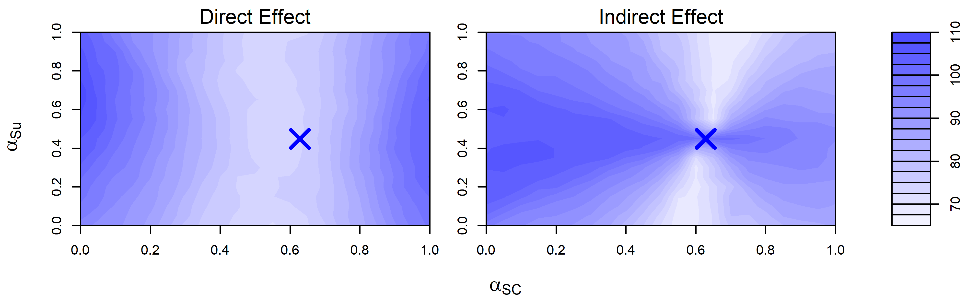
Figure 1 shows the relative efficiency of our estimators and the inverse probability-weighted estimators. Across all treatment allocation strategies α=(αSC,αSu)\alpha=(\alpha_{\rm SC},\alpha_{\rm Su}), our estimator τ~\widetilde{\tau} is more efficient than the inverse probability-weighted estimator, with our estimator showing 68.46 to 109.26 times improvements in efficiency. This empirical result corroborates our theoretical result in Corollary 4.2 on the semiparametric efficiency of our estimator. We also notice that for the direct effect, efficiency gain does not change when αSu\alpha_{\rm Su} varies. In contrast, for the spillover effect, the efficiency gain does change with both αSU\alpha_{\rm SU} and αSC\alpha_{\rm SC}.

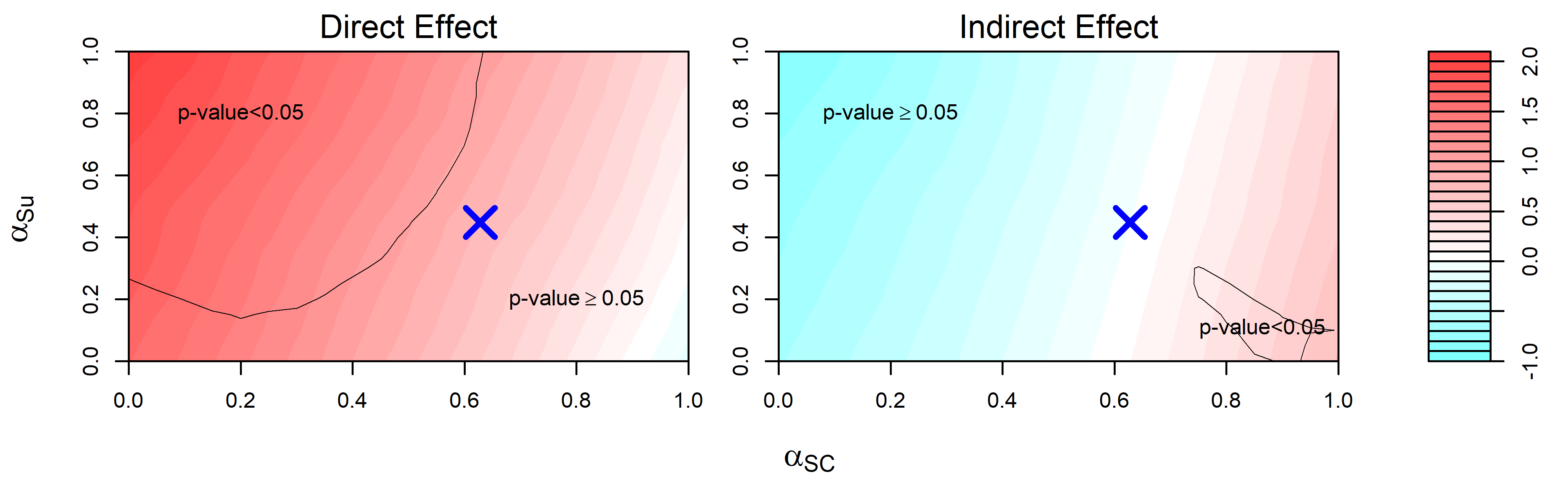
Figure 2 shows the direct and spillover effect estimates based on the proposed efficient estimator. In general, the direct effect tends to be positive and significant for large αSu\alpha_{\rm Su}. But, the spillover effect has a phase-transition behavior along αSC\alpha_{\rm SC} where the effect is negative for small αSC\alpha_{\rm SC} and positive for large αSC\alpha_{\rm SC}. Practically speaking, the analysis suggests that enrolling more students in San Cristobal induce a more stronger spillover effect towards their siblings compared to doing it in Suba. But, enrolling more students in Suba can yield a more positive direct effect compared to doing it in San Cristobal. Combined, San Cristobal may have stronger sibling spillover effects compared to Suba, potentially providing information about structuring conditional cash transfer programs to take advantage of the differences in how the treatment affects attendance rates in the two regions.
Refer to caption
Figure 1: Relative efficiency between the proposed efficient estimator and the inverse probability-weighted estimator in Liu et al. 2016. The colors on the plot show the ratio of the variance of the efficient estimator to the variance of the inverse probability-weighted estimator, with darker colors indicating higher values of the ratio, or more improvements in efficiency for the proposed estimator. The left and right plots show the relative efficiencies for the direct and spillover effects, respectively. The xx-axis varies the treatment allocation strategy αSC\alpha_{\rm SC} for San Cristobal and the yy-axis varies the treatment allocation strategy αSu\alpha_{\rm Su} for Suba. The blue cross (×\times) is the original treatment probability from the experiment, α∗=(0.628,0.449)\alpha^{*}=(0.628,0.449).
Refer to caption
Figure 2: Effect estimates in percentage points using the proposed efficient estimator. The colors on the left and right plots show the magnitude and sign of the estimated effects, respectively. The xx-axis varies the treatment allocation strategy αSC\alpha_{\rm SC} for San Cristobal and the yy-axis varies the treatment allocation strategy αSu\alpha_{\rm Su} for Suba. We also show the regions where the effects are significant at level 0.05. The blue cross (×\times) is the original treatment probability from the experiment, α∗=(0.628,0.449)\alpha^{*}=(0.628,0.449).

6 Discussion

This paper proposes a framework to derive globally and locally efficient influence functions of network treatment effects in T\mathrm{T}. Our results complement the rich set of results on efficient estimation of treatment effects without interference and establish that one of the estimator in Liu et al. 2019 is locally efficient. We also discuss results on adaptivity, notably that the efficiency is not affected by the knowledge of the propensity score, but can be affected by the knowledge of the interference pattern. Finally, we show other parametric and nonparametric estimation methods that, under some assumptions, can achieve the efficiency bound. Our empirical application corroborates our theoretical results, showing that our estimators have smaller standard errors than those by Liu et al. 2016.

We take a moment to discuss the strengths and limitations of our framework using model (1), notably the restrictions on cluster size. While our framework is useful to characterize optimality of estimators in small cluster settings, say twins, households, classrooms, small villages or clinics, or certain settings in neuroimaging (Luo et al. 2012), it is not appropriate in settings where the cluster size is large compared to the number of individuals per cluster, say states, i.e. 50 states/clusters, with many individuals per cluster, or hospital systems. In fact, if Oi{{O}}_{i} grows in dimension, Liu and Hudgens 2014 showed that the limiting distributions of popular estimators under partial interference are no longer asymptotically normal. In this setting, we likely need a dimension-reducing assumption to make the dependence among units theoretically manageable, say by assuming the dependence is characterized by known summary functions of peers’ data; see van der Laan 2014, Sofrygin and van der Laan 2016, and Ogburn et al. 2017 for examples. A limitation of such works is that, as suggested in our result concerning adaptivity with respect to the interference pattern, efficiency depends on this summarizing function. That is, an estimator that was efficient under one summarizing function may no longer be efficient, and potentially inconsistent, under a different summarizing function. Ultimately, these limitations can be thought of as a cost for obtaining efficient estimators in large networks. In contrast, if the number of study units in a cluster is not large and thus model (1) is plausible, we do not have to make assumptions about how peers influence each other in order to construct our estimators.

Overall, no asymptotic framework for networks is uniformly superior and investigators should use estimators based on the data at hand. In particular, with the current theory, if investigators are working with large online networks and they know how peers might affect each other, the estimators by Sofrygin and van der Laan 2016 and Ogburn et al. 2017 show promise. On the other hand, if investigators are working with studies involving twins, households, small villages, or neuroimaging, and they have insufficient knowledge about how units affect each other, our framework and the proposed optimal estimators show promise.

Supplementary Material

This document contains supplementary materials for “Efficient Semiparametric Estimation of Network Treatment Effects Under Partial Interference.” Section A presents additional results related to the main paper. Section B proves the theorems stated in the main paper. Section C proves the theorems and lemmas stated in Section A.

Appendix A Additional Results

In this section, we introduce additional results which are related to the main paper.

A.1 Comments about Model (1)

In relation to others works, model (1) is a generalization of Example 1 of Bickel and Kwon 2001 where P(k)P^{(k)} in their notation is equivalent to our P⁡(Oi∣Li=k)P({{O}}_{i}\mid L_{i}=k) and Example 2 of McNeney and Wellner 2000 where we allow for different densities. Also, (1) complements Sofrygin and van der Laan 2016 who worked under general interference and as such, had to assume (a) a single, known summary function of peers’ data and (b) conditional on the summary function, a study unit’s data Oi​jO_{ij} are independent and identically distributed; see their assumptions (A2), (A3), and (B1). In our setup, we leverage the partial interference structure where we have independence across clusters and as such, allow for different non-parametric functionals to model dependencies within a cluster. Additionally, while (1) is a type of mixture model, the goal in our paper is not to identify or estimate unknown mixture labels LiL_{i} typical in mixture modeling. Instead, we use LiL_{i} as a technical device to embed studies under partial interference into (1) and hence LiL_{i} is known by construction; see the next paragraph for some examples. Finally, when K=1K=1 and there is only one study unit in a cluster, (1) reduces to the usual independent and identically distributed setting without interference; in fact, as K>1K>1 and there are at least two study unit per cluster, our asymptotic framework has both independent and identically distributed and non-independent and non-identically distributed components. Specifically, we observe independent and identically distributed copies of Oi{{O}}_{i} within each cluster type, but elements of the vector Oi{{O}}_{i} may exhibit arbitrary dependence structure and each cluster type may have different densities. As we’ll see below, this blend of independent and identically distributed and non-independent and identically distributed structure leads to efficient influence functions that look similar, but not identical, to efficient influence functions under independence.

As mentioned in the main manuscript, many, but not all, studies under partial interference can be modeled by (1). For example, when the number of study units within each cluster is fixed, such as studies involving dyads (Rosenbaum 2007; Elwert and Christakis 2008; Nickerson 2008; Lu and Anderson 2015; Baird et al. 2018), or when the number of study units is bounded, as in households surveys or in neuroimaging studies (Cowling et al. 2009; Luo et al. 2012), we can define LiL_{i} by the size of each cluster and model these studies as data generated from (1); see Barkley et al. 2020 and Basse and Feller 2018 for other examples of organizing clusters by size. More broadly, so long as clusters are organized by finite number of LiL_{i}s, studies under partial interference can be reasonably modeled by (1). However, if the number of study units in a cluster is growing and there is no restrictions on P⁡(Oi∣Li)P({{O}}_{i}\mid L_{i}), our setting does not apply. In such settings, one likely requires assumptions on P⁡(Oi∣Li)P({{O}}_{i}\mid L_{i}) to reduce its dimension, say by assuming the aforementioned summary function to represent peers’ data. If we also make such assumptions, (1) can be used. In general, in settings where the size of the cluster grows, assumptions are likely necessary to deal with the curse of dimensionality and, perhaps more importantly, to define a reasonable efficiency or variance-based criterion.

A.2 Details of Section 2

We show that the direct effect τDE​(α)=E⁡{Y¯i​(1,α)−Y¯i​(0,α)}{\tau}^{\rm DE}(\alpha)={E}\big\{\overline{Y}_{i}(1\,;\,\alpha)-\overline{Y}_{i}(0\,;\,\alpha)\big\} and the indirect effect τIE​(α,α′)=E⁡{Y¯i​(1,α)−Y¯i​(0,α)}{\tau}^{\rm IE}(\alpha,\alpha^{\prime})={E}\big\{\overline{Y}_{i}(1\,;\,\alpha)-\overline{Y}_{i}(0\,;\,\alpha)\big\}, which are counterpart of the direct and indirect effects defined in Hudgens and Halloran 2008 under an infinite population framework, belong to T{\rm T}. If we choose the weights wk{{w}}_{k} as

wk​(ai,α)=1Mk​[{𝟙​(ai​1=1)−𝟙​(ai​1=0)}​π​(ai⁡(−1),α){𝟙​(ai​j=1)−𝟙​(ai​j=0)}​π​(ai⁡(−j),α){𝟙​(ai​Mk=1)−𝟙​(ai​Mk=0)}​π​(ai⁡(−Mk),α)],\displaystyle{{w}}_{k}({{a}}_{i}\,;\,\alpha)=\frac{1}{M_{k}}\begin{bmatrix}\big\{\mathbbm{1}\big(a_{i1}=1)-\mathbbm{1}\big(a_{i1}=0)\big\}\pi({{a}}_{i(-1)}\,;\,\alpha)\\ \vdots\\ \big\{\mathbbm{1}\big(a_{ij}=1)-\mathbbm{1}\big(a_{ij}=0)\big\}\pi({{a}}_{i(-j)}\,;\,\alpha)\\ \vdots\\ \big\{\mathbbm{1}\big(a_{iM_{k}}=1)-\mathbbm{1}\big(a_{iM_{k}}=0)\big\}\pi({{a}}_{i(-M_{k})}\,;\,\alpha)\end{bmatrix}\ , (11)

this leads to the following for θk\theta_{k}:

θk\displaystyle\theta_{k} =1Mk[∑ai⁡(−1)E[{Yi​1(ai​1=1,ai⁡(−1))−Yi​1(ai​1=0,ai⁡(−1))}π(ai⁡(−1);α)|Li=k]+⋯\displaystyle=\frac{1}{M_{k}}\bigg[\sum_{{{a}}_{i(-1)}}{E}\Big[\big\{Y_{i1}(a_{i1}=1,{{a}}_{i(-1)})-Y_{i1}(a_{i1}=0,{{a}}_{i(-1)})\big\}\pi({{a}}_{i(-1)}\,;\,\alpha)\,\Big|\,L_{i}=k\Big]+\cdots
+∑ai⁡(−j)E[{Yi​j(ai​j=1,ai⁡(−j))−Yi​j(ai​j=0,ai⁡(−j))}π(ai⁡(−j);α)|Li=k]+⋯\displaystyle\hskip 28.45274pt+\sum_{{{a}}_{i(-j)}}{E}\Big[\big\{Y_{ij}(a_{ij}=1,{{a}}_{i(-j)})-Y_{ij}(a_{ij}=0,{{a}}_{i(-j)})\big\}\pi({{a}}_{i(-j)}\,;\,\alpha)\,\Big|\,L_{i}=k\Big]+\cdots
+∑ai⁡(−Mk)E[{Yi​Mk(ai​Mk=1,ai⁡(−Mk))−Yi​Mk(ai​Mk=0,ai⁡(−Mk))}π(ai⁡(−Mk);α)|Li=k]]\displaystyle\hskip 28.45274pt+\sum_{{{a}}_{i(-M_{k})}}{E}\Big[\big\{Y_{iM_{k}}(a_{iM_{k}}=1,{{a}}_{i(-M_{k})})-Y_{iM_{k}}(a_{iM_{k}}=0,{{a}}_{i(-M_{k})})\big\}\pi({{a}}_{i(-M_{k})}\,;\,\alpha)\,\Big|\,L_{i}=k\Big]\bigg]
=1Mk​[E⁡{Y¯i​1​(1,α)+⋯+Y¯i​Mk​(1,α)∣Li=k}−E⁡{Y¯i​1​(0,α)+⋯+Y¯i​Mk​(0,α)∣Li=k}]\displaystyle=\frac{1}{M_{k}}\Big[{E}\big\{\overline{Y}_{i1}(1;\alpha)+\cdots+\overline{Y}_{iM_{k}}(1;\alpha)\mid L_{i}=k\big\}-{E}\big\{\overline{Y}_{i1}(0\,;\,\alpha)+\cdots+\overline{Y}_{iM_{k}}(0\,;\,\alpha)\mid L_{i}=k\big\}\Big]
=E⁡{Y¯i​(1,α)−Y¯i​(0,α)∣Li=k}\displaystyle={E}\big\{\overline{Y}_{i}(1\,;\,\alpha)-\overline{Y}_{i}(0\,;\,\alpha)\mid L_{i}=k\big\}

where the second identity is from the definition of Y¯i​j​(a,α)\overline{Y}_{ij}(a\,;\,\alpha) and the last identity is from the definition of Y¯i​(a,α)\overline{Y}_{i}(a\,;\,\alpha). Thus, the weight in (11) makes the parameter θk\theta_{k} equal to the direct effect in cluster type kk. If we also take vk​(pk)=pk=P⁡(Li=k)v_{k}(p_{k})=p_{k}=P(L_{i}=k), then τ\tau is the same as the direct effect E⁡{Y¯i​(1,α)−Y¯i​(0,α)}{E}\big\{\overline{Y}_{i}(1\,;\,\alpha)-\overline{Y}_{i}(0\,;\,\alpha)\big\}, i.e.

τ=∑k=1Kpk​θk=∑k=1KP⁡(Li=k)​E​{Y¯i​(1,α)−Y¯i​(0,α)∣Li=k}=E⁡{Y¯i​(1,α)−Y¯i​(0,α)}.\displaystyle\tau=\sum_{k=1}^{K}p_{k}\theta_{k}=\sum_{k=1}^{K}P(L_{i}=k){E}\big\{\overline{Y}_{i}(1\,;\,\alpha)-\overline{Y}_{i}(0\,;\,\alpha)\mid L_{i}=k\big\}={E}\big\{\overline{Y}_{i}(1\,;\,\alpha)-\overline{Y}_{i}(0\,;\,\alpha)\big\}\ .

If we choose the weights wk{{w}}_{k} as

wk​(ai,α)=1Mk​[𝟙​(ai​1=0)​{π⁡(ai⁡(−1),α)−π⁡(ai⁡(−1),α′)}𝟙​(ai​j=0)​{π⁡(ai⁡(−j),α)−π⁡(ai⁡(−j),α′)}𝟙​(ai​Mk=0)​{π⁡(ai⁡(−Mk),α)−π⁡(ai⁡(−Mk),α′)}],\displaystyle{{w}}_{k}({{a}}_{i}\,;\,\alpha)=\frac{1}{M_{k}}\begin{bmatrix}\mathbbm{1}(a_{i1}=0)\{\pi({{a}}_{i(-1)}\,;\,\alpha)-\pi({{a}}_{i(-1)}\,;\,\alpha^{\prime})\}\\ \vdots\\ \mathbbm{1}(a_{ij}=0)\{\pi({{a}}_{i(-j)}\,;\,\alpha)-\pi({{a}}_{i(-j)}\,;\,\alpha^{\prime})\}\\ \vdots\\ \mathbbm{1}(a_{iM_{k}}=0)\{\pi({{a}}_{i(-M_{k})}\,;\,\alpha)-\pi({{a}}_{i(-M_{k})}\,;\,\alpha^{\prime})\}\end{bmatrix}\ , (12)

this leads to the following for θk\theta_{k}:

θk\displaystyle\theta_{k} =1Mk[∑ai⁡(−1)E[Yi​1(ai​1=0,ai⁡(−1)){π(ai⁡(−1);α)−π(ai⁡(−1);α′)}|Li=k]+⋯\displaystyle=\frac{1}{M_{k}}\bigg[\sum_{{{a}}_{i(-1)}}{E}\Big[Y_{i1}(a_{i1}=0,{{a}}_{i(-1)})\big\{\pi({{a}}_{i(-1)}\,;\,\alpha)-\pi({{a}}_{i(-1)}\,;\,\alpha^{\prime})\big\}\,\Big|\,L_{i}=k\Big]+\cdots
+∑ai⁡(−Mk)E[Yi​Mk(ai​Mk=0,ai⁡(−Mk)){π(ai⁡(−Mk);α)−π(ai⁡(−Mk);α′)}|Li=k]]\displaystyle\hskip 28.45274pt+\sum_{{{a}}_{i(-M_{k})}}{E}\Big[Y_{iM_{k}}(a_{iM_{k}}=0,{{a}}_{i(-M_{k})})\big\{\pi({{a}}_{i(-M_{k})}\,;\,\alpha)-\pi({{a}}_{i(-M_{k})}\,;\,\alpha^{\prime})\big\}\,\Big|\,L_{i}=k\Big]\bigg]
=1Mk​[E⁡{Y¯i​1​(0,α)+⋯+Y¯i​Mk​(0,α)∣Li=k}−E⁡{Y¯i​1​(0,α′)+⋯+Y¯i​Mk​(0,α′)∣Li=k}]\displaystyle=\frac{1}{M_{k}}\Big[{E}\big\{\overline{Y}_{i1}(0;\alpha)+\cdots+\overline{Y}_{iM_{k}}(0;\alpha)\mid L_{i}=k\big\}-{E}\big\{\overline{Y}_{i1}(0\,;\,\alpha^{\prime})+\cdots+\overline{Y}_{iM_{k}}(0\,;\,\alpha^{\prime})\mid L_{i}=k\big\}\Big]
=E⁡{Y¯i​(0,α)−Y¯i​(0,α′)∣Li=k}\displaystyle={E}\big\{\overline{Y}_{i}(0\,;\,\alpha)-\overline{Y}_{i}(0\,;\,\alpha^{\prime})\mid L_{i}=k\big\}

Thus, the weight in (12) makes the parameter θk\theta_{k} equal to the indirect effect in cluster type kk. If we also take vk​(pk)=pk=P⁡(Li=k)v_{k}(p_{k})=p_{k}=P(L_{i}=k), then τ\tau is the same as the indirect effect E⁡{Y¯i​(0,α)−Y¯i​(0,α′)}{E}\big\{\overline{Y}_{i}(0\,;\,\alpha)-\overline{Y}_{i}(0\,;\,\alpha^{\prime})\big\}, i.e.

τ=∑k=1Kpk​θk=∑k=1KP⁡(Li=k)​E​{Y¯i​(0,α)−Y¯i​(0,α′)∣Li=k}=E⁡{Y¯i​(0,α)−Y¯i​(0,α′)}.\displaystyle\tau=\sum_{k=1}^{K}p_{k}\theta_{k}=\sum_{k=1}^{K}P(L_{i}=k){E}\big\{\overline{Y}_{i}(0\,;\,\alpha)-\overline{Y}_{i}(0\,;\,\alpha^{\prime})\mid L_{i}=k\big\}={E}\big\{\overline{Y}_{i}(0\,;\,\alpha)-\overline{Y}_{i}(0\,;\,\alpha^{\prime})\big\}\ .

Next, we introduce the details of the asymptotic embedding of network treatment effects.

Lemma A.1 (Asymptotic Embedding of Network Treatment Effects).

Suppose that the potential outcome Yi​(ai){{Y}}_{i}({{a}}_{i}) and the type variable LiL_{i} of cluster ii are a random sample from a super-population satisfying condition (1) in the main paper where Oi{{O}}_{i} is replaced with Yi​(ai){{Y}}_{i}({{a}}_{i}). Consider a network causal estimand τF​(α,α′){\tau}^{F}({\alpha},{\alpha}^{\prime}) which is a linear combination of individual average potential outcome Y¯i​j​(a,αk)\overline{Y}_{ij}(a\,;\,\alpha_{k}) defined in Section 2.1 of the main paper, i.e.,

τF​(α,α′)=1N​∑i=1N∑k=1K𝟙​(Li=k)​∑j=1Mk{C1​j​k​Y¯i​j​(1,αk)+C2​j​k​Y¯i​j​(0,αk)+C3​j​k​Y¯i​j​(1,αk′)+C4​j​k​Y¯i​j​(0,αk′)}.\displaystyle{\tau}^{F}({\alpha},{\alpha}^{\prime})=\frac{1}{N}\sum_{i=1}^{N}\sum_{k=1}^{K}\mathbbm{1}(L_{i}=k)\sum_{j=1}^{M_{k}}\left\{\begin{matrix}C_{1jk}\overline{Y}_{ij}(1\,;\,\alpha_{k})+C_{2jk}\overline{Y}_{ij}(0\,;\,\alpha_{k})\hskip 56.9055pt\\ \hskip 56.9055pt+C_{3jk}\overline{Y}_{ij}(1\,;\,\alpha^{\prime}_{k})+C_{4jk}\overline{Y}_{ij}(0\,;\,\alpha^{\prime}_{k})\end{matrix}\right\}\ .

Here, Cℓ​j​kC_{\ell jk}s (ℓ=1,2,3,4,j=1,…,Mk,k=1,…,K)(\ell=1,2,3,4,j=1,\ldots,M_{k},k=1,\ldots,K) are fixed constants. If (i) KK and MkM_{k} are bounded by a constant for all k=1,…,Kk=1,\ldots,K and (ii) the conditional expectation E⁡{Yi​(ai)∣Li=k}{E}\big\{{{Y}}_{i}({{a}}_{i})\mid L_{i}=k\big\} is finite for all ai∈𝒜⁡(Mk){{a}}_{i}\in\mathcal{A}(M_{k}) and k=1,…,Kk=1,\ldots,K, then there exists τ⁡(α,α′)∈T{\tau}({\alpha},{\alpha}^{\prime})\in\mathrm{T} for all α{\alpha} and α′{\alpha}^{\prime} where τF​(α,α′){\tau}^{F}({\alpha},{\alpha}^{\prime}) converges to τ⁡(α,α′){\tau}({\alpha},{\alpha}^{\prime}) in probability as N→∞N\rightarrow\infty.

The proof of Lemma A.1 is in Section C.1. Lemma A.1 generalizes this observation and shows that under certain growth conditions, finite sample causal estimands in partial interference can be asymptotically embedded into our framework. We remark that while Lemma A.1 was restricted to estimands with α\alpha-policy weights, we can pick any causal estimand where the weights in T\mathrm{T} are not based on α\alpha-policies. So long as these weights are pre-specified a-priori and satisfy the constraints of T\mathrm{T}, the results below will still hold.

A.3 Details of Section 3.1 in the Main Paper

We introduce Lemma A.2, which is a key step to proving Theorem 3.

Lemma A.2 (Semiparametric Efficiency Bound of θ∗{\theta}^{*}).

Let θ∗=(θ1∗,…,θK∗){\theta}^{*}=({\theta}_{1}^{*},\ldots,{\theta}_{K}^{*}) where θk∗∈Θk{\theta}_{k}^{*}\in\Theta_{k}. Under the conditions in Assumption 2.1 in the main paper, the efficient influence function of θ∗=(θ1∗,…,θK∗)T{\theta}^{*}=({\theta}_{1}^{*},\ldots,{\theta}_{K}^{*})^{\mathrm{\scriptscriptstyle T}} in model ℳNP\mathcal{M}_{{\rm NP}}, denoted by φ⁡(θ∗)=(φ1​(θ1∗),…,φK​(θK∗))T\varphi({\theta}^{*})=\big(\varphi_{1}({\theta}_{1}^{*}),\ldots,\varphi_{K}({\theta}_{K}^{*})\big)^{\mathrm{\scriptscriptstyle T}}, is

φk​(θk∗)=𝟙​(Li=k)pk∗​[∑ai∈𝒜⁡(Mk)wkT​(ai,Xi)​[𝟙​(Ai=ai)e∗​(ai∣Xi,k)​{Yi−g∗​(ai,Xi,k)}+g∗​(ai,Xi,k)]−θk∗]\displaystyle\varphi_{k}({\theta}_{k}^{*})=\frac{\mathbbm{1}(L_{i}=k)}{p_{k}^{*}}\Bigg[\sum_{{{a}}_{i}\in\mathcal{A}(M_{k})}\hskip-7.11317pt{{w}}_{k}^{\mathrm{\scriptscriptstyle T}}({{a}}_{i},{{X}}_{i})\bigg[\frac{\mathbbm{1}({{A}}_{i}={{a}}_{i})}{e^{*}({{a}}_{i}\mid{{X}}_{i},k)}\Big\{{{Y}}_{i}-{{g}}^{*}({{a}}_{i},{{X}}_{i},k)\Big\}+{{g}}^{*}({{a}}_{i},{{X}}_{i},k)\bigg]-{\theta}_{k}^{*}\Bigg]

and the corresponding semiparametric efficiency bound of θ∗{\theta}^{*} in model ℳNP\mathcal{M}_{{\rm NP}}, denoted by var​{φ⁡(θ∗)}{\rm var}\big\{\varphi({\theta}^{*})\big\}, is var⁡{φ⁡(θ∗)}=diag​[SEB1​(θ1∗),…,SEBK​(θK∗)]{\rm var}\big\{\varphi({\theta}^{*})\big\}=\text{diag}\big[\text{SEB}_{1}\big({\theta}_{1}^{*}\big),\ldots,\text{SEB}_{K}\big({\theta}_{K}^{*}\big)\big] with

SEBk(θk∗)=1pk∗E[∑ai∈𝒜⁡(Mk)wkT​(ai,Xi)​Σ∗​(ai,Xi,k)​wk​(ai,Xi)e∗​(ai∣Xi,k)\displaystyle\text{SEB}_{k}\big({\theta}_{k}^{*}\big)=\frac{1}{p_{k}^{*}}{E}\bigg[\hskip-1.42271pt\sum_{{{a}}_{i}\in\mathcal{A}(M_{k})}\hskip-8.5359pt\frac{{{w}}_{k}^{\mathrm{\scriptscriptstyle T}}({{a}}_{i},{{X}}_{i})\Sigma^{*}({{a}}_{i},{{X}}_{i},k){{w}}_{k}({{a}}_{i},{{X}}_{i})}{e^{*}({{a}}_{i}\mid{{X}}_{i},k)}
+{∑ai∈𝒜⁡(Mk)wkT(ai,Xi)g∗(ai,Xi,k)−θk∗}2|Li=k].\displaystyle\hskip 142.26378pt+\bigg\{\hskip-1.42271pt\sum_{{{a}}_{i}\in\mathcal{A}(M_{k})}\hskip-8.5359pt{{w}}_{k}^{\mathrm{\scriptscriptstyle T}}({{a}}_{i},{{X}}_{i}){{g}}^{*}({{a}}_{i},{{X}}_{i},k)-{\theta}_{k}^{*}\bigg\}^{2}\,\bigg|\,L_{i}=k\bigg]\ .

Moreover, φ⁡(θ∗)\varphi({\theta}^{*}) is also the efficient influence function of θ∗{\theta}^{*} in model ℳNP,e∗={PO,L∈ℳNP∣e∗​ is known}\mathcal{M}_{{\rm NP},e^{*}}=\big\{P_{O,L}\in\mathcal{M}_{{\rm NP}}\mid e^{*}\text{ is known}\big\}.

The proof is presented in Section C.2.

We consider the case of known pk∗p_{k}^{*}s and derive the efficient influence function and the semiparametric efficiency bound for τ∗∈T{\tau}^{*}\in\mathrm{T}, which is the extension of Theorem 3.1 in the main paper. The result is formally presented in Theorem A.1.

Theorem A.1 (Semiparametric Efficiency Bound of τ∗∈T{\tau}^{*}\in\mathrm{T} under known pk∗p_{k}^{*}).

Let τ∗∈T{\tau}^{*}\in\mathrm{T} be the parameter defined in (3) in the main paper. Suppose that the conditions in Assumption 2.1 in the main paper hold. If pk∗p_{k}^{*}s are known, the efficient influence function of τ∗{\tau}^{*} in model ℳNP\mathcal{M}_{{\rm NP}} (and in model ℳNP,e∗\mathcal{M}_{{\rm NP},e^{*}}) is

φ⁡(τ∗)\displaystyle\varphi({\tau}^{*}) =∑k=1Kvk​(pk∗)​φk​(θk∗)\displaystyle=\sum_{k=1}^{K}v_{k}(p_{k}^{*})\varphi_{k}({\theta}_{k}^{*})

where φk\varphi_{k} is defined in Lemma A.2. Moreover, the semiparametric efficiency bound of τ∗{\tau}^{*} in model ℳNP\mathcal{M}_{{\rm NP}} is

var⁡{φ⁡(τ∗)}=∑k=1Kvk​(pk∗)2​SEBk​(θk∗)\displaystyle{\rm var}\big\{\varphi({\tau}^{*})\big\}=\sum_{k=1}^{K}v_{k}(p_{k}^{*})^{2}\text{SEB}_{k}({\theta}_{k}^{*})

where SEBk\text{SEB}_{k} is defined in Lemma A.2.

The proof is presented in Section C.3. Compared to the result of Theorem 3.1 in the main paper, the semiparametric efficiency bound under known pk∗p_{k}^{*} is smaller than or equal to the semiparametric efficiency bound under unknown pk∗p_{k}^{*}. That is, we gain efficiency because of the knowledge of pk∗p_{k}^{*}.

We show that the equation (4) can be used to construct a doubly robust estimator. Specifically, for each cluster type kk, let θ^k​(e′,g′)\widehat{{\theta}}_{k}(e^{\prime},{{g}}^{\prime}) be the solution to an estimating equation constructed from (4) by using some e′e^{\prime} and g′{{g}}^{\prime}, i.e.,

θ^k(e′,g′)=1Nk∑i:Li=k∑ai∈𝒜⁡(Mk)wkT(ai,Xi)[𝟙​(Ai=ai)e′​(ai∣Xi,k){Yi−g′(ai,Xi,k)}+g′(ai,Xi,k)].\displaystyle\widehat{{\theta}}_{k}(e^{\prime},{{g}}^{\prime})=\frac{1}{N_{k}}\sum_{i:L_{i}=k}\sum_{{{a}}_{i}\in\mathcal{A}(M_{k})}{{w}}_{k}^{\mathrm{\scriptscriptstyle T}}({{a}}_{i},{{X}}_{i})\Bigg[\frac{\mathbbm{1}({{A}}_{i}={{a}}_{i})}{e^{\prime}({{a}}_{i}\mid{{X}}_{i},k)}\Big\{{{Y}}_{i}-{{g}}^{\prime}({{a}}_{i},{{X}}_{i},k)\Big\}+{{g}}^{\prime}({{a}}_{i},{{X}}_{i},k)\Bigg]\ .

We define an estimator of τ∗{\tau}^{*} based on θ^k​(e′,g′)\widehat{{\theta}}_{k}(e^{\prime},{{g}}^{\prime}) as

τ^​(e′,g′)=v^T​θ^​(e′,g′)=∑k=1Kv^k​θ^k​(e′,g′),θ^​(e′,g′)=(θ^1​(e′,g′),…,θ^K​(e′,g′))T\displaystyle\widehat{{\tau}}(e^{\prime},{{g}}^{\prime})=\widehat{{{v}}}^{\mathrm{\scriptscriptstyle T}}\widehat{{\theta}}(e^{\prime},{{g}}^{\prime})=\sum_{k=1}^{K}\widehat{v}_{k}\widehat{{\theta}}_{k}(e^{\prime},{{g}}^{\prime})\quad,\quad\widehat{{\theta}}(e^{\prime},{{g}}^{\prime})=\big(\widehat{{\theta}}_{1}(e^{\prime},{{g}}^{\prime}),\ldots,\widehat{{\theta}}_{K}(e^{\prime},{{g}}^{\prime})\big)^{\mathrm{\scriptscriptstyle T}} (13)

where v^=(v^1,…,v^K)T\widehat{{{v}}}=\big(\widehat{v}_{1},\ldots,\widehat{v}_{K}\big)^{\mathrm{\scriptscriptstyle T}} is an unbiased estimator of v⁡(p∗){{v}}({{p}}^{*}) constructed based on the variable LiL_{i}. Theorem A.2 shows that τ^​(e′,g′)\widehat{{\tau}}(e^{\prime},{{g}}^{\prime}) is unbiased even if the propensity score or the outcome model, but not both, is mis-specified.

Theorem A.2 (Double Robustness of τ^​(e′,g′)\widehat{{\tau}}(e^{\prime},{{g}}^{\prime})).

Suppose that the conditions in Assumption 2.1 hold and v^\widehat{{{v}}} is an unbiased estimator of v⁡(p∗){{v}}({{p}}^{*}). Then, τ^\widehat{{\tau}} is doubly robust in the sense that τ^​(e′,g′)\widehat{{\tau}}(e^{\prime},{{g}}^{\prime}) is an unbiased estimator of τ{\tau}, i.e., E⁡{τ^​(e′,g′)}=τ∗{E}\big\{\widehat{{\tau}}(e^{\prime},{{g}}^{\prime})\big\}={\tau}^{*}, if either e′=e∗e^{\prime}=e^{*} or g′=g∗{{g}}^{\prime}={{g}}^{*}.

The proof is presented in Section C.4. We believe Theorem A.2 can be used as a basis to construct robust machine learning and cross-fitting estimators (Chernozhukov et al. 2018) under partial interference where half of the clusters are used to non-parametrically estimate ee and g{{g}} and the other half is used to estimate τ{\tau}; see Section 4.2 in th main paper.

Finally, we conclude the section by briefly discussing estimators of direct and indirect effects under our framework. Specifically, after some algebra, the efficient influence functions of direct and indirect effects are

φ⁡(τDE​(α))=∑k=1K𝟙​(Li=k)​{ψk​(1,e∗,g∗,α)−ψk​(0,e∗,g∗,α)}−τDE​(α)\displaystyle\varphi\big({\tau}^{\rm DE}(\alpha)\big)=\sum_{k=1}^{K}\mathbbm{1}(L_{i}=k)\Big\{\psi_{k}(1,e^{*},{{g}}^{*},\alpha)-\psi_{k}(0,e^{*},{{g}}^{*},\alpha)\Big\}-{\tau}^{\rm DE}(\alpha)
φ⁡(τIE​(α,α′))=∑k=1K𝟙​(Li=k)​{ψk​(0,e∗,g∗,α)−ψk​(0,e∗,g∗,α′)}−τIE​(α,α′)\displaystyle\varphi\big({\tau}^{\rm IE}(\alpha,\alpha^{\prime})\big)=\sum_{k=1}^{K}\mathbbm{1}(L_{i}=k)\Big\{\psi_{k}(0,e^{*},{{g}}^{*},\alpha)-\psi_{k}(0,e^{*},{{g}}^{*},\alpha^{\prime})\Big\}-{\tau}^{\rm IE}(\alpha,\alpha^{\prime})

where

ψk​(a,e,g,α)=1Mk​∑j=1Mk∑ai∈𝒜⁡(Mk)ai​j=a[𝟙​(Ai=ai)e⁡(ai∣Xi,k)​{Yi​j−gj​(ai,Xi,k)}+gj​(ai,Xi,k)]​π​(ai⁡(−j),α).\displaystyle\psi_{k}(a,e,{{g}},\alpha)=\frac{1}{M_{k}}\sum_{j=1}^{M_{k}}\sum_{\begin{subarray}{c}{{a}}_{i}\in\mathcal{A}(M_{k})\\ a_{ij}=a\end{subarray}}\Bigg[\frac{\mathbbm{1}({{A}}_{i}={{a}}_{i})}{e({{a}}_{i}\mid{{X}}_{i},k)}\Big\{Y_{ij}-g_{j}({{a}}_{i},{{X}}_{i},k)\Big\}+g_{j}({{a}}_{i},{{X}}_{i},k)\Bigg]\pi({{a}}_{i(-j)}\,;\,\alpha)\ .

Here gjg_{j} is jjth component of g{{g}}, i.e., the outcome regression of individual jj. Also, by following (13), the efficient influence functions above lead to the following doubly robust estimators of τDE​(α){\tau}^{\rm DE}(\alpha) and τIE​(α,α′){\tau}^{\rm IE}(\alpha,\alpha^{\prime}).

τ^DE​(α,e′,g′)=∑k=1Kp^k⋅θ^kDE​(α,e′,g′),τ^IE​(α,α′,e′,g′)=∑k=1Kp^k⋅θ^kIE​(α,α′,e′,g′)\displaystyle\widehat{{\tau}}^{{\rm DE}}(\alpha\,;\,e^{\prime},{{g}}^{\prime})=\sum_{k=1}^{K}\widehat{p}_{k}\cdot\widehat{{\theta}}_{k}^{{\rm DE}}(\alpha\,;\,e^{\prime},{{g}}^{\prime}),\ \widehat{{\tau}}^{{\rm IE}}(\alpha,\alpha^{\prime}\,;\,e^{\prime},{{g}}^{\prime})=\sum_{k=1}^{K}\widehat{p}_{k}\cdot\widehat{{\theta}}_{k}^{{\rm IE}}(\alpha,\alpha^{\prime}\,;\,e^{\prime},{{g}}^{\prime})

where e′e^{\prime} and g′{{g}}^{\prime} are pre-specified functions of the propensity score and the outcome regression, respectively, θ^kDE(α;e′,g′)=Nk−1∑i:Li=k{ψk(1,e′,g′,α)−ψk(0,e′,g′,α)}\widehat{{\theta}}_{k}^{{\rm DE}}(\alpha\,;\,e^{\prime},{{g}}^{\prime})=N_{k}^{-1}\sum_{i:L_{i}=k}\big\{\psi_{k}(1,e^{\prime},{{g}}^{\prime},\alpha)-\psi_{k}(0,e^{\prime},{{g}}^{\prime},\alpha)\big\}, and θ^kIE(α,α′;e′,g′)=Nk−1∑i:Li=k{ψk(0,e′,g′,α)−ψk(0,e′,g′,α′)}\widehat{{\theta}}_{k}^{{\rm IE}}(\alpha,\alpha^{\prime}\,;\,e^{\prime},{{g}}^{\prime})=N_{k}^{-1}\sum_{i:L_{i}=k}\big\{\psi_{k}(0,e^{\prime},{{g}}^{\prime},\alpha)-\psi_{k}(0,e^{\prime},{{g}}^{\prime},\alpha^{\prime})\big\}. Moreover, e′e^{\prime} and g′{{g}}^{\prime} can be replaced with estimates that satisfy Theorem 3.2 in the main paper. As a consequence, we obtain τ^DE​(α)\widehat{{\tau}}^{\rm DE}(\alpha) and τ^IE​(α,α′)\widehat{{\tau}}^{\rm IE}(\alpha,\alpha^{\prime}) in (5) in the main paper.

A.4 Details of Section 3.2 in the Main Paper

To prove Theorem 3.2, we present Lemma A.3 and the regularity conditions (R1)–(R4).

Lemma A.3 (M-Estimators of θ∗{\theta}^{*}).

Suppose Assumption 2.1 and the following regularity conditions (R1)–(R4) hold for the estimating equation Ψ⁡(θ,β)=(ΨθT​(θ,β),ΨβT​(β))T\Psi({\theta},\beta)=\big(\Psi_{\theta}^{\mathrm{\scriptscriptstyle T}}({\theta},{\beta}),\Psi_{\beta}^{\mathrm{\scriptscriptstyle T}}({\beta})\big)^{\mathrm{\scriptscriptstyle T}}: (R1) (θ,β)({\theta},{\beta}) lies in an open set Ω0\Omega_{0}, which is a subset of a compact, finite dimensional Euclidean space. Also, βe{\beta}_{e} and βg{\beta}_{g} are variationally independent; (R2) Ψ⁡(θ,β)\Psi({\theta},{\beta}) is twice continuously differentiable in (θ,β)({\theta},{\beta}); (R3) There is a unique value (θ∗,β†)({\theta}^{*},{\beta}^{\dagger}) where (i) E⁡{Ψ⁡(θ∗,β†)}=0E\big\{\Psi({\theta}^{*},{\beta}^{\dagger})\big\}=0, (ii) E⁡{‖Ψ⁡(θ∗,β†)‖22}<∞E\big\{\big\|\Psi({\theta}^{*},{\beta}^{\dagger})\big\|_{2}^{2}\big\}<\infty, and (iii) E⁡{∂Ψ⁡(θ∗,β†)/∂(θ,β)}E\big\{\partial\Psi({\theta}^{*},{\beta}^{\dagger})/\partial({\theta},{\beta})\big\} exists and is non-singular; (R4) Every element of the second order partial derivatives ∂2Ψ⁡(θ,β)/{∂(θ,β)​∂(θ,β)T}\partial^{2}\Psi({\theta},{\beta})/\{\partial({\theta},{\beta})\partial({\theta},{\beta})^{\mathrm{\scriptscriptstyle T}}\} are dominated by a fixed integrable function for all (θ,β)({\theta},{\beta}) in a neighborhood of (θ∗,β†)({\theta}^{*},{\beta}^{\dagger}). Let β†{\beta}^{\dagger} be the probability limit of β^\widehat{{\beta}}. Then, under model ℳe∪ℳg\mathcal{M}_{e}\cup\mathcal{M}_{g}, we have

N​(θ^−θ∗)=1N​∑i=1NφPar​(θ∗,β†)+oP​(1)\displaystyle\sqrt{N}\big(\widehat{{\theta}}-{\theta}^{*}\big)=\frac{1}{\sqrt{N}}\sum_{i=1}^{N}\varphi^{\rm Par}({\theta}^{*},{\beta}^{\dagger})+o_{P}(1)

where φPar​(θ∗,β†)=[φ1Par​(θ1∗,β†),…,φKPar​(θK∗,β†)]T\varphi^{\rm Par}\big({\theta}^{*},{\beta}^{\dagger}\big)=\big[\varphi_{1}^{\rm Par}\big({\theta}_{1}^{*},{\beta}^{\dagger}\big)\ ,\ \ldots\ ,\ \varphi_{K}^{\rm Par}\big({\theta}_{K}^{*},{\beta}^{\dagger}\big)\big]^{\mathrm{\scriptscriptstyle T}} and

φkPar​(θk∗,β†)=1pk∗​[Ψθ,k​(θk∗,β†)−E⁡{∂Ψθ,k​(θk∗,β†)∂βT}​[E⁡{Ψβ​(β†)∂βT}]−1​Ψβ​(β†)].\displaystyle\varphi_{k}^{\rm Par}\big({\theta}_{k}^{*},{\beta}^{\dagger}\big)=\frac{1}{p_{k}^{*}}\bigg[\Psi_{{\theta},k}({\theta}_{k}^{*},{\beta}^{\dagger})-{E}\bigg\{\frac{\partial\Psi_{{\theta},k}({\theta}_{k}^{*},{\beta}^{\dagger})}{\partial{\beta}^{\mathrm{\scriptscriptstyle T}}}\bigg\}\bigg[{E}\bigg\{\frac{\Psi_{\beta}({\beta}^{\dagger})}{\partial{\beta}^{\mathrm{\scriptscriptstyle T}}}\bigg\}\bigg]^{-1}\Psi_{\beta}({\beta}^{\dagger})\bigg]\ .

The proof is presented in Section C.5.

A.5 Details of Adaptive Estimation in Section 3 in the Main Paper

This section investigates two properties related to adaptive estimation under partial interference, adaption to the knowledge about the propensity score and adaption to the knowledge about the inference pattern/covariance structure. We remark that without interference, the aforementioned works on the augmented inverse probability-weighted estimator for the average treatment effect showed that the estimator adapts to the knowledge about the propensity score and the variance.

First, suppose the propensity score e∗e^{*} is known as in a two-stage randomized experiment from Hudgens and Halloran 2008. In adaptive estimation, we want to understand whether having this knowledge can lead to more efficient estimation of τ∗{\tau}^{*}. Unfortunately, but in alignment with the results without interference, Theorem A.3 shows that the estimator from Theorem 3.2 in the main paper that does not use this information still achieves the semiparametric efficiency bound of τ∗{\tau}^{*} when the propensity score is known.

Theorem A.3 (Adaptation to Known Propensity Score).

Suppose conditions in Theorem 3.2 in the main paper hold. Let τ^\widehat{{\tau}} be the estimator in Theorem 3.2 in the main paper where ee and gg are estimated from ℳe∩ℳg\mathcal{M}_{e}\cap\mathcal{M}_{g}. Then, the asymptotic variance of τ^\widehat{{\tau}} achieves the semiparametric efficiency bound of τ∗{\tau}^{*} under ℳNP,e∗={PO,L∈ℳNP∣e∗​ known}\mathcal{M}_{{\rm NP},e^{*}}=\big\{P_{O,L}\in\mathcal{M}_{{\rm NP}}\mid e^{*}\text{ known}\big\}.

The proof is presented in Section C.6. In words, the efficient estimators in Theorem 3.2 in the main paper that does not use the knowledge that the propensity score is known can adapt and still achieve the best possible variance regardless of the knowledge of e∗e^{*}.

Second, without interference, a somewhat under-emphasized fact about the augmented inverse probability-weighted estimator of the average treatment effect is that the estimator remains efficient irrespective of the investigator’s knowledge about the true variance of the outcome, i.e. the estimator adapts. We ask a similar type of question under partial interference, specifically whether having certain a priori knowledge about the interference pattern/exposure mapping (Aronow and Samii 2017) would affect efficiencies of the proposed estimators. Unlike the case without interference, we show that in a setting where the true model has no interference, but the investigator, out of caution or lack of awareness, uses the estimators in (5) that take interference into account, the estimators are consistent, but no longer efficient; in short, the estimators do not adapt to the underlying true interference pattern.

Formally, consider an “interference-free” model space ℳNoInt⊆ℳNP\mathcal{M}_{{\rm NoInt}}\subseteq\mathcal{M}_{{\rm NP}} which is equal to

ℳNoInt={PO,L∈ℳNP|\displaystyle\mathcal{M}_{{\rm NoInt}}=\big\{P_{{{O}},L}\in\mathcal{M}_{{\rm NP}}\,\big|\, Yi​j|(Ai=ai,Xi=x,Li=k)=Yi​j|(Ai​j=ai​j,Xi=x,Li=k)\displaystyle Y_{ij}\mid({{A}}_{i}={{a}}_{i},{{X}}_{i}={{x}},L_{i}=k)=Y_{ij}\mid(A_{ij}=a_{ij},{{X}}_{i}={{x}},L_{i}=k)
almost surely for all ai∈𝒜(Mk),x∈𝒳(k),k=1,…,K}.\displaystyle\text{almost surely for all }{{a}}_{i}\in\mathcal{A}(M_{k}),\ {{x}}\in\mathcal{X}(k),\ k=1,\ldots,K\big\}\ .

Next, we introduce ℳ~NoInt\widetilde{\mathcal{M}}_{\rm NoInt}, which is defined as

ℳ~NoInt={PO,L∈ℳNP|\displaystyle\widetilde{\mathcal{M}}_{\rm NoInt}=\big\{P_{{{O}},L}\in\mathcal{M}_{{\rm NP}}\,\big|\, E⁡(Yi​j∣Ai,Xi,Li=k)=E⁡(Yi​j∣Ai′,Xi,Li=k),\displaystyle{E}\big(Y_{ij}\mid{{A}}_{i},{{X}}_{i},L_{i}=k\big)={E}\big(Y_{ij}\mid{{A}}_{i}^{\prime},{{X}}_{i},L_{i}=k\big)\ ,
where ​Ai,Ai′∈𝒜⁡(Mk)​ such that ​Ai​j=Ai​j′,j=1,…,Mk,\displaystyle\text{where }{{A}}_{i},{{A}}_{i}^{\prime}\in\mathcal{A}(M_{k})\text{ such that }A_{ij}=A_{ij}^{\prime}\ ,\ j=1,\ldots,M_{k}\ ,
Xi∈𝒳(k),k=1,…,K}.\displaystyle{{X}}_{i}\in\mathcal{X}(k)\ ,\ k=1,\ldots,K\big\}\ .

ℳ~NoInt\widetilde{\mathcal{M}}_{\rm NoInt} is a collection of models without first-order (i.e., in mean) interference. Trivially, ℳ~NoInt\widetilde{\mathcal{M}}_{\rm NoInt} includes ℳNoInt\mathcal{M}_{\rm NoInt}, the collection of “truly” no interference models because of the nested relationship imposed by the definition of each set.

Lastly, we define the “interference-free” outcome model ℳg,NoInt⊆ℳg∩ℳNoInt\mathcal{M}_{g,{\rm NoInt}}\subseteq\mathcal{M}_{g}\cap\mathcal{M}_{{\rm NoInt}} which is equal to

ℳg,NoInt={PO,L∈ℳg∩ℳNoInt|\displaystyle\mathcal{M}_{g,{\rm NoInt}}=\big\{P_{{{O}},L}\in\mathcal{M}_{g}\cap\mathcal{M}_{{\rm NoInt}}\,\big|\, gj​(ai,x,k,βg)=gj​(ai′,x,k,βg)​ for all ​j=1,…,Mk,\displaystyle g_{j}({{a}}_{i},{{x}},k\,;\,{\beta}_{g})=g_{j}({{a}}_{i}^{\prime},{{x}},k\,;\,{\beta}_{g})\text{ for all }j=1,\ldots,M_{k},\
ai,ai′∈𝒜(Mk) with ai​j=ai​j′,x∈𝒳(k),k=1,…,K}.\displaystyle{{a}}_{i},{{a}}_{i}^{\prime}\in\mathcal{A}(M_{k})\text{ with }a_{ij}=a_{ij}^{\prime},\ {{x}}\in\mathcal{X}(k),\ k=1,\ldots,K\big\}\ .

Under model ℳg,NoInt\mathcal{M}_{g,{\rm NoInt}} and the consistency condition (A1), the outcome regression of unit jj in cluster ii does not depend on the treatment status of ii’s peers so that gj∗​(ai,x,k)g_{j}^{*}({{a}}_{i},{{x}},k) is a function only of unit jj’s treatment assignment ai​ja_{ij}. Furthermore, we introduce a function gjNoInt​(ai​j,xi,k)g^{\rm NoInt}_{j}(a_{ij},{{x}}_{i},k) which is the same as gj∗​(ai,xi,k)g_{j}^{*}({{a}}_{i},{{x}}_{i},k), but the former emphasizes the lack of dependence on ai⁡(−j){{a}}_{i(-j)}. Therefore, under model ℳg,NoInt\mathcal{M}_{g,{\rm NoInt}}, we obtain the following equivalence at the true parameter βg{\beta}_{g} for all ai⁡(−j)∈𝒜⁡(Mk−1){{a}}_{i(-j)}\in\mathcal{A}(M_{k}-1).

gjNoInt​(ai​j,xi,k)=gjPar,NoInt​(ai​j,xi,k,βg∗)=gj∗​(ai,xi,k)=gj​(ai,xi,k,βg∗).\displaystyle g^{\rm NoInt}_{j}(a_{ij},{{x}}_{i},k)=g^{\rm Par,NoInt}_{j}(a_{ij},{{x}}_{i},k\,;\,{\beta}_{g}^{*})=g_{j}^{*}({{a}}_{i},{{x}}_{i},k)=g_{j}({{a}}_{i},{{x}}_{i},k\,;\,{\beta}_{g}^{*})\ . (14)

We study the behavior of the direct effect and the indirect effect across the counterfactual parameters under model ℳNoInt\mathcal{M}_{{\rm NoInt}}. Let the average treatment effect τATE{\tau}^{\rm ATE} where τATE=∑k=1Kpk∗​θkATE{\tau}^{\rm ATE}=\sum_{k=1}^{K}p_{k}^{*}{\theta}_{k}^{\rm ATE} and θkATE=Mk−1​∑j=1MkE⁡{Yi​j​(ai​j=1)−Yi​j​(ai​j=0)∣Li=k}{\theta}_{k}^{\rm ATE}=M_{k}^{-1}\sum_{j=1}^{M_{k}}{E}\big\{Y_{ij}(a_{ij}=1)-Y_{ij}(a_{ij}=0)\mid L_{i}=k\big\}. Here Yi​j​(ai​j=a)Y_{ij}(a_{ij}=a) is the potential outcome of unit jj in cluster ii when the unit’s treatment status is a∈{0,1}a\in\{0,1\}. Lemma A.4 shows that τDE​(α){\tau}^{\rm DE}(\alpha) and τIE​(α,α′){\tau}^{\rm IE}(\alpha,\alpha^{\prime}) defined in the main paper are the same as τATE{\tau}^{\rm ATE} and 00, respectively, in model ℳ~NoInt\widetilde{\mathcal{M}}_{\rm NoInt}.

Lemma A.4.

Suppose that the true model belongs to ℳ~NoInt\widetilde{\mathcal{M}}_{\rm NoInt}. Then, τDE​(α)=τATE{\tau}^{\rm DE}(\alpha)={\tau}^{\rm ATE} and τIE​(α,α′)=0{\tau}^{\rm IE}(\alpha,\alpha^{\prime})=0 for all α,α′∈(0,1)\alpha,\alpha^{\prime}\in(0,1).

The proof is presented in Section C.7. Note that the above Lemma also holds after replacing ℳ~NoInt\widetilde{\mathcal{M}}_{\rm NoInt} with ℳNoInt{\mathcal{M}}_{\rm NoInt} because of the nested relationships. Importantly, this implies that we can use the proposed locally efficient estimators of the direct and indirect effects in Section 3.2. Theorem A.4 shows that while these estimators remain consistent, they do not adapt to the no-interference structure and are no longer efficient.

Theorem A.4 (Non-Adaptation to Exposure Mapping).

Suppose conditions in Theorem 3.2 hold. Let ee and gg be estimated from ℳe∩ℳg\mathcal{M}_{e}\cap\mathcal{M}_{g}. Then, for all α,α′∈(0,1)\alpha,\alpha^{\prime}\in(0,1), τ^DE​(α)\widehat{{\tau}}^{{\rm DE}}(\alpha) and τ^IE​(α,α′)\widehat{{\tau}}^{{\rm IE}}(\alpha,\alpha^{\prime}) are consistent for τATE{\tau}^{\rm ATE} and 00, respectively, under ℳe∩ℳg,NoInt\mathcal{M}_{e}\cap\mathcal{M}_{g,{\rm NoInt}}. Also, unless the outcome and the propensity score models satisfy invariance conditions in Assumption A.1 below, τ^DE​(α)\widehat{{\tau}}^{{\rm DE}}(\alpha) does not achieve the semiparametric efficiency bound for τATE{\tau}^{\rm ATE} under ℳNoInt\mathcal{M}_{{\rm NoInt}}.

The proof is presented in Section C.8. Theorem A.4 shows that if the investigator uses estimators that account for interference, but the true data has no interference, the estimators are consistent, but generally inefficient; in short, the investigator pays a price in terms of efficiency.

The additional invariance conditions are given as follows.

Assumption A.1 (Invariance Condition).

Suppose the outcome regression and the propensity score satisfy the following invariance conditions, respectively.

  • (a)

    (Propensity Score): For all α∈(0,1)\alpha\in(0,1) and ai⁡(−j)∈𝒜⁡(Mk−1){{a}}_{i(-j)}\in\mathcal{A}(M_{k}-1), π⁡(ai⁡(−j),α)​Σj​j∗​(ai,x,k)/e∗​(ai∣x,k)\pi({{a}}_{i(-j)}\,;\,\alpha)\Sigma_{jj}^{*}({{a}}_{i},{{x}},k)/e^{*}({{a}}_{i}\mid{{x}},k) is identical where Σj​j∗​(ai,x,k)\Sigma_{jj}^{*}({{a}}_{i},{{x}},k) is the jjth diagonal element of Σ∗​(ai,x,k)\Sigma^{*}({{a}}_{i},{{x}},k).

  • (b)

    (Outcome Regression): For all j=1,…,Mkj=1,\ldots,M_{k}, yi⁡(−j)∈ℝMk−1{{y}}_{i(-j)}\in\mathbb{R}^{M_{k}-1}, ai∈𝒜⁡(Mk){{a}}_{i}\in\mathcal{A}(M_{k}), xi∈𝒳⁡(k){{x}}_{i}\in\mathcal{X}(k), k=1,…,Kk=1,\ldots,K, the following identities hold under model ℳNoInt\mathcal{M}_{{\rm NoInt}}.

    E⁡(Yi​j|Yi⁡(−j)=yi⁡(−j),Ai=ai,Xi=xi,Li=k)\displaystyle{E}\big(Y_{ij}\,\big|\,{{Y}}_{i(-j)}={{y}}_{i(-j)},{{A}}_{i}={{a}}_{i},{{X}}_{i}={{x}}_{i},L_{i}=k\big)
    =E⁡(Yi​j|Ai=ai,Xi=xi,Li=k)=E⁡(Yi​j|Ai​j=ai​j,Xi=xi,Li=k).\displaystyle={E}\big(Y_{ij}\,\big|\,{{A}}_{i}={{a}}_{i},{{X}}_{i}={{x}}_{i},L_{i}=k\big)={E}\big(Y_{ij}\,\big|\,A_{ij}=a_{ij},{{X}}_{i}={{x}}_{i},L_{i}=k\big)\ .

    Note that the second identity is trivial under model ℳNoInt\mathcal{M}_{{\rm NoInt}}.

Condition (a) of Assumption A.1 states that the propensity score is invariant to α\alpha and ai{{a}}_{i}; note that condition (b) holds under randomized experiment where pr⁡(Ai​j=1)=α{\rm pr}(A_{ij}=1)=\alpha and Σj​j∗​(ai,x,k)\Sigma_{jj}^{*}(a_{i},x,k) does not depend on aia_{i}.

Condition (b) of Assumption A.1 roughly states that the peers’ outcomes do not provide any information about one’s own outcome. The first immediate result under condition (a) is that the conditional variance matrix Σ∗​(ai,xi,k)=var⁡(Yi∣Ai=ai,Xi=xi,Li=k)\Sigma^{*}({{a}}_{i},{{x}}_{i},k)={\rm var}({{Y}}_{i}\mid{{A}}_{i}={{a}}_{i},{{X}}_{i}={{x}}_{i},L_{i}=k) is diagonal. Lemma A.5 formally states this.

Lemma A.5.

Let the (i,j)(i,j)th entry of Σ∗​(ai,xi,k)\Sigma^{*}({{a}}_{i},{{x}}_{i},k) be Σi​j∗​(ai,xi,k)\Sigma_{ij}^{*}({{a}}_{i},{{x}}_{i},k). Suppose that condition (a) of Assumption A.1 holds. Then, Σ∗​(ai,xi,k)\Sigma^{*}({{a}}_{i},{{x}}_{i},k) is diagonal and Σj​j∗​(ai,xi,k)\Sigma_{jj}^{*}({{a}}_{i},{{x}}_{i},k) does not depend on ai⁡(−j){{a}}_{i(-j)}. That is, Σ∗​(ai,xi,k)=diag⁡[Σ11∗​(ai​1,xi,k),…,ΣMk​Mk∗​(ai​Mk,xi,k)]\Sigma^{*}({{a}}_{i},{{x}}_{i},k)={\rm diag}\big[\Sigma_{11}^{*}(a_{i1},{{x}}_{i},k),\ldots,\Sigma_{M_{k}M_{k}}^{*}(a_{iM_{k}},{{x}}_{i},k)\big].

The proof is presented in Section C.9.

Next, we derive the efficient influence function of τATE{\tau}^{\rm ATE} in model ℳNoInt\mathcal{M}_{{\rm NoInt}} under Assumption A.1. Lemma A.6 formally shows the result.

Lemma A.6.

Suppose that the conditions in Assumption 2.1 in the main paper and Assumption A.1 hold. Then, the efficient influence function of τATE{\tau}^{\rm ATE} in model ℳNoInt\mathcal{M}_{{\rm NoInt}}, denoted by φ⁡(τATE)\varphi({\tau}^{\rm ATE}), is

φ(τATE)=∑k=1K𝟙(Li=k)[1Mk∑j=1Mk[{𝟙(Ai​j=1)−𝟙(Ai​j=0)}Yi​j−gjNoInt​(Ai​j,Xi,k)ej∗​(Ai​j∣Xi,k)\displaystyle\varphi({\tau}^{\rm ATE})=\sum_{k=1}^{K}\mathbbm{1}(L_{i}=k)\bigg[\frac{1}{M_{k}}\sum_{j=1}^{M_{k}}\bigg[\Big\{\mathbbm{1}(A_{ij}=1)-\mathbbm{1}(A_{ij}=0)\Big\}\frac{Y_{ij}-g^{\rm NoInt}_{j}(A_{ij},{{X}}_{i},k)}{e_{j}^{*}(A_{ij}\mid{{X}}_{i},k)}
+{gjNoInt(1,Xi,k)−gjNoInt(0,Xi,k)}]]−τATE.\displaystyle\hskip 170.71652pt+\Big\{g^{\rm NoInt}_{j}(1,{{X}}_{i},k)-g^{\rm NoInt}_{j}(0,{{X}}_{i},k)\Big\}\bigg]\bigg]-{\tau}^{\rm ATE}\ .

where gjNoIntg^{\rm NoInt}_{j} is defined in (14) and ej∗e_{j}^{*} is the conditional probability of Ai​jA_{ij} being assigned to a certain treatment indicator; i.e.,

ej∗​(a∣Xi,k)=∑ai∈𝒜⁡(Mk)𝟙​(ai​j=a)​e∗​(ai∣Xi,k)=pr⁡(Ai​j=a∣Xi,Li=k).\displaystyle e_{j}^{*}(a\mid{{X}}_{i},k)=\sum_{{{a}}_{i}\in\mathcal{A}(M_{k})}\mathbbm{1}(a_{ij}=a)e^{*}({{a}}_{i}\mid{{X}}_{i},k)={\rm pr}(A_{ij}=a\mid{{X}}_{i},L_{i}=k)\ .

Therefore, the semiparametric efficiency bound of τATE{\tau}^{\rm ATE} in model ℳNoInt\mathcal{M}_{{\rm NoInt}} is

E⁡{φ​(τATE)2}\displaystyle{E}\big\{\varphi({\tau}^{\rm ATE})^{2}\big\} =∑k=1Kpk∗Mk2​∑j=1MkE⁡{Σj​j∗​(1,Xi,k)ej∗​(1∣Xi,k)+Σj​j∗​(0,Xi,k)ej∗​(0∣Xi,k)|Li=k}\displaystyle=\sum_{k=1}^{K}\frac{p_{k}^{*}}{M_{k}^{2}}\sum_{j=1}^{M_{k}}{E}\bigg\{\frac{\Sigma_{jj}^{*}(1,{{X}}_{i},k)}{e_{j}^{*}(1\mid{{X}}_{i},k)}+\frac{\Sigma_{jj}^{*}(0,{{X}}_{i},k)}{e_{j}^{*}(0\mid{{X}}_{i},k)}\,\bigg|\,L_{i}=k\bigg\}
+E⁡[[∑k=1K𝟙​(Li=k)Mk​∑j=1Mk{gjNoInt​(1,Xi,k)−gjNoInt​(0,Xi,k)}−τATE]2]\displaystyle+{E}\bigg[\bigg[\sum_{k=1}^{K}\frac{\mathbbm{1}(L_{i}=k)}{M_{k}}\sum_{j=1}^{M_{k}}\Big\{g^{\rm NoInt}_{j}(1,{{X}}_{i},k)-g^{\rm NoInt}_{j}(0,{{X}}_{i},k)\Big\}-{\tau}^{\rm ATE}\bigg]^{2}\bigg]

where Σj​j∗​(ai​j,xi,k)\Sigma_{jj}^{*}(a_{ij},{{x}}_{i},k) is defined in Lemma A.5.

The proof is presented in Section C.10. Note that φ⁡(τATE)\varphi({\tau}^{\rm ATE}) is an extension of Hahn 1998 to clustered data. Specifically, if all units are independent and identically distributed, this leads to K=1K=1, M1=1M_{1}=1, and j=1j=1. Therefore, the efficient influence function of φ⁡(τATE)\varphi({\tau}^{\rm ATE}) and the semiparametric efficiency bound of τATE{\tau}^{\rm ATE} reduce to

φ⁡(τATE)\displaystyle\varphi({\tau}^{\rm ATE}) =𝟙​(Ai​1=1)e1∗​(1∣Xi,1)​{Yi​1−g1NoInt​(1,Xi,1)}−𝟙​(Ai​1=0)e1∗​(0∣Xi,1)​{Yi​1−g1NoInt​(0,Xi,1)}\displaystyle=\frac{\mathbbm{1}(A_{i1}=1)}{e_{1}^{*}(1\mid{{X}}_{i},1)}\Big\{Y_{i1}-g^{\rm NoInt}_{1}(1,{{X}}_{i},1)\Big\}-\frac{\mathbbm{1}(A_{i1}=0)}{e_{1}^{*}(0\mid{{X}}_{i},1)}\Big\{Y_{i1}-g^{\rm NoInt}_{1}(0,{{X}}_{i},1)\Big\}
+{g1NoInt​(1,Xi,1)−g1NoInt​(0,Xi,1)−τATE},\displaystyle\hskip 85.35826pt+\Big\{g^{\rm NoInt}_{1}(1,{{X}}_{i},1)-g^{\rm NoInt}_{1}(0,{{X}}_{i},1)-{\tau}^{\rm ATE}\Big\}\ ,
E⁡{φ​(τATE)2}\displaystyle{E}\big\{\varphi({\tau}^{\rm ATE})^{2}\big\} =E⁡[Σj​j∗​(1,Xi,1)e1∗​(1∣Xi,1)+Σj​j∗​(0,Xi,1)e1∗​(0∣Xi,1)+{g1NoInt​(1,Xi,1)−g1NoInt​(0,Xi,1)−τATE}2]\displaystyle={E}\bigg[\frac{\Sigma_{jj}^{*}(1,{{X}}_{i},1)}{e_{1}^{*}(1\mid{{X}}_{i},1)}+\frac{\Sigma_{jj}^{*}(0,{{X}}_{i},1)}{e_{1}^{*}(0\mid{{X}}_{i},1)}+\Big\{g^{\rm NoInt}_{1}(1,{{X}}_{i},1)-g^{\rm NoInt}_{1}(0,{{X}}_{i},1)-{\tau}^{\rm ATE}\Big\}^{2}\bigg]

which are equivalent to the results under no interference originally introduced in Hahn 1998.

Finally, we conduct a small simulation study to visually illustrate Theorem A.4. Suppose we only have one cluster type (i.e., K=1K=1) and the cluster size is two (i.e., M1=2M_{1}=2). We assume the true model has no interference and has the following form.

(Model of ​X)Xi​j∼i.i.d.N⁡(0,1)(Model of ​A)Ai​j∼i.i.d.Ber​(pA∗),pA∗∈{0.3,0.5,0.7},\displaystyle(\text{Model of }X)\ \ X_{ij}\stackrel{{\scriptstyle\text{i.i.d.}}}{{\sim}}N(0,1)\quad\quad(\text{Model of }A)\ \ A_{ij}\stackrel{{\scriptstyle\text{i.i.d.}}}{{\sim}}\text{Ber}(p_{A}^{*})\ ,\ p_{A}^{*}\in\big\{0.3,0.5,0.7\big\}\ ,
(Model of ​Y)Yi​j=1+3​Ai​j+2​Xi​j+0.5​Xi⁡(−j)+ϵi​j,ϵi​j∼i.i.d.N⁡(0,1).\displaystyle(\text{Model of }Y)\ \ Y_{ij}=1+3A_{ij}+2X_{ij}+0.5X_{i(-j)}+\epsilon_{ij}\ ,\quad\epsilon_{ij}\stackrel{{\scriptstyle\text{i.i.d.}}}{{\sim}}N(0,1)\ .

Briefly, each unit has one pre-treatment covariate, following a standard normal distribution, and pre-treatment covariates are independent from each other. The treatment is completely randomized with probability pr⁡(Ai​j=1)=pA∗∈{0.3,0.5,0.7}{\rm pr}(A_{ij}=1)=p_{A}^{*}\in\{0.3,0.5,0.7\}. The outcome variable is generated from a regression model that has no interference between units, but depends on peers’ covariate Xi⁡(−j)X_{i(-j)}; our numerical results will be similar if we remove the peer’s covariate in the outcome model. We generate N=10,000N=10,000 samples from the simulation model and compute τ^DE​(α)\widehat{{\tau}}^{\rm DE}(\alpha) and τ^IE​(α,0.9)\widehat{{\tau}}^{\rm IE}(\alpha,0.9) that allow for interference. We compute these two estimates for a range of policy parameter from α=0.01\alpha=0.01 to α=0.99\alpha=0.99. We repeat the simulation 1,0001,000 times.

Before we discuss our numerical results, we first study what is expected from our theory by calculating the theoretical variance of τ^DE​(α)\widehat{{\tau}}^{\rm DE}(\alpha) using Theorem 3.2 and the semiparametric efficiency bound of τATE{\tau}^{\rm ATE}.

var​{τ^DE​(α)}\displaystyle{\rm var}\big\{\widehat{{\tau}}^{\rm DE}(\alpha)\big\} =12​{(1−α)2(1−pA∗)2+α2+(1−α)2pA∗​(1−pA∗)+α2pA∗2},E⁡{φ​(τATE)2}=12​pA∗​(1−pA∗).\displaystyle=\frac{1}{2}\bigg\{\frac{(1-\alpha)^{2}}{(1-p_{A}^{*})^{2}}+\frac{\alpha^{2}+(1-\alpha)^{2}}{p_{A}^{*}(1-p_{A}^{*})}+\frac{\alpha^{2}}{p_{A}^{*2}}\bigg\}\ ,\ {E}\big\{\varphi({\tau}^{\rm ATE})^{2}\big\}=\frac{1}{2p_{A}^{*}(1-p_{A}^{*})}\ .

Notice that var​{τ^DE​(α)}{\rm var}\big\{\widehat{{\tau}}^{\rm DE}(\alpha)\big\} is uniquely minimized at α=pA∗\alpha=p_{A}^{*}, which satisfies the invariance condition, and becomes the semiparametric efficiency bound of τATE{\tau}^{\rm ATE}. Specifically, var⁡{τ^DE​(pA∗)}{\rm var}\big\{\widehat{{\tau}}^{\rm DE}(p_{A}^{*})\big\} is minimized at pA∗=0.5p_{A}^{*}=0.5 and maximized at either (α,pA∗)=(0.99,0.3)(\alpha,p_{A}^{*})=(0.99,0.3) or (α,pA∗)=(0.01,0.7)(\alpha,p_{A}^{*})=(0.01,0.7).

Next, Figure 3 summarizes the numerical results from our simulation. We see that the empirical biases of τ^DE​(α)\widehat{{\tau}}^{\rm DE}(\alpha) are negligible and centered around zero, agreeing with the theory developed in Theorem A.4-(i); the empirical biases of τ^IE​(α,0.9)\widehat{{\tau}}^{\rm IE}(\alpha,0.9), which are not reported, are also negligible. Also, the empirical variances of τ^DE​(α)\widehat{{\tau}}^{\rm DE}(\alpha) agrees with our theoretical discussion above where the variances are minimized when α=pA∗\alpha=p_{A}^{*} and maximized when α\alpha is near the “edges” of the plots. In short, the estimator is consistent, but is not always efficient when the true data has no interference. More generally, the results highlight that unlike non-interference settings, knowing the interference pattern may affect the efficiency of an estimator designed for interference and future work should be cognizant of this phenomena.

Figure 3: Graphical illustration of adaption under no interference. Left, middle, and right plots correspond to treatment assignment probabilities pA∗=0.3p_{A}^{*}=0.3, 0.50.5, and 0.70.7, respectively. Top plots show the empirical biases of direct effect estimates and bottom plots show the theoretical and empirical variances of direct effect estimates. The xx axis represents the policy parameter α\alpha and the yy axis represents either bias or variance. The black solid lines( ) are the theoretical biases and variances of τ^DE​(α)\widehat{{\tau}}^{\rm DE}(\alpha). The red solid lines( ) are the empirical biases and variances of τ^DE​(α)\widehat{{\tau}}^{\rm DE}(\alpha) from the simulation. The blue dashed lines(     ) are the semiparametric efficiency bounds of τATE{\tau}^{\rm ATE}. The filled triangle () is the policy parameter α\alpha that equals pA∗p_{A}^{*}.

A.6 Details of Section 4 in the Main Paper

Based on model in Section 4.1, we conduct a small simulation study to illustrate the theoretical results. Suppose we have two cluster types (i.e., K=2K=2) and the cluster size of the two types is three and four (i.e., M1=3M_{1}=3 and M2=4M_{2}=4). We assume that the true data generating model has the following form.

(Model of ​X)\displaystyle(\text{Model of }X) Xi​j=(Ci,Wi​j)T=(Ci,Wi​j​1,Wi​j​2)T,\displaystyle{{X}}_{ij}=(C_{i},W_{ij})^{\mathrm{\scriptscriptstyle T}}=(C_{i},W_{ij1},W_{ij2})^{\mathrm{\scriptscriptstyle T}},\
Ci∼i.i.d.N⁡(0,1),Wi​j​1∼i.i.dBer​(0.5),Wi​j​2∼i.i.d.N⁡(0,1),\displaystyle C_{i}\stackrel{{\scriptstyle\text{i.i.d.}}}{{\sim}}N(0,1),\ W_{ij1}\stackrel{{\scriptstyle i.i.d}}{{\sim}}\text{Ber}(0.5),\ W_{ij2}\stackrel{{\scriptstyle\text{i.i.d.}}}{{\sim}}N(0,1),\
Ci,Wi​j​1, and ​Wi​j​2​ are independent\displaystyle C_{i},W_{ij1},\text{ and }W_{ij2}\text{ are independent}
(Model of ​A)\displaystyle(\text{Model of }A) logit⁡{pr⁡(Ai​j=1∣Xi,Li=k,bi)}=[1,Wi​jT,∑ℓ≠jWi​ℓT]​βe,k+bi\displaystyle{\rm logit}\big\{{\rm pr}(A_{ij}=1\mid{{X}}_{i},L_{i}=k,b_{i})\big\}=\Big[1,{{W}}_{ij}^{\mathrm{\scriptscriptstyle T}},\sum_{\ell\neq j}{{W}}_{i\ell}^{\mathrm{\scriptscriptstyle T}}\Big]{\beta}_{e,k}+b_{i}
βe,1=[−1.25,2,0.3,0.2,0.1]T,βe,2=[−1,1.25,0.2,0.15,0.1]T,\displaystyle{\beta}_{e,1}=\big[-1.25,2,0.3,0.2,0.1\big]^{\mathrm{\scriptscriptstyle T}}\ ,\ {\beta}_{e,2}=\big[-1,1.25,0.2,0.15,0.1\big]^{\mathrm{\scriptscriptstyle T}}\ ,\
bi∼i.i.d.N⁡(0,0.25)\displaystyle b_{i}\stackrel{{\scriptstyle\text{i.i.d.}}}{{\sim}}N(0,0.25)
(Model of ​Y)\displaystyle(\text{Model of }Y) Yi​j=[1,Ai​j,∑ℓ≠jAi​ℓ,Ai​j​Ci,(∑ℓ≠jAi​ℓ)​Ci,Xi​jT,∑ℓ≠jWi​ℓT]​βg,k+ξi+ϵi​j\displaystyle Y_{ij}=\Big[1,A_{ij},\sum_{\ell\neq j}A_{i\ell},A_{ij}C_{i},\Big(\sum_{\ell\neq j}A_{i\ell}\Big)C_{i},{{X}}_{ij}^{\mathrm{\scriptscriptstyle T}},\sum_{\ell\neq j}{{W}}_{i\ell}^{\mathrm{\scriptscriptstyle T}}\Big]{\beta}_{g,k}+\xi_{i}+\epsilon_{ij}
βg,1=[2,3,0.8,1,0.5,0.8,−1,0.5,−0.3,0.15]T,\displaystyle{\beta}_{g,1}=\big[2,3,0.8,1,0.5,0.8,-1,0.5,-0.3,0.15\big]^{\mathrm{\scriptscriptstyle T}}\ ,\
βg,2=[1,2,0.4,0.5,0.3,0.6,−0.8,0.4,−0.2,0.1]T,\displaystyle{\beta}_{g,2}=\big[1,2,0.4,0.5,0.3,0.6,-0.8,0.4,-0.2,0.1\big]^{\mathrm{\scriptscriptstyle T}}\ ,\
ξi∼i.i.d.N⁡(0,0.1),ϵi​j∼i.i.d.N⁡(0,1)\displaystyle\xi_{i}\stackrel{{\scriptstyle\text{i.i.d.}}}{{\sim}}N(0,0.1)\ ,\ \epsilon_{ij}\stackrel{{\scriptstyle\text{i.i.d.}}}{{\sim}}N(0,1)

Each study unit has thee pre-treatment covariates, one binary (Wi​j​1W_{ij1}) and two continuous (CiC_{i} and Wi​j​2W_{ij2}), where Wi​j​1W_{ij1} and Wi​j​2W_{ij2} are individual-level covariates and CiC_{i} is a cluster-level covariate and the three covariates are independent of each other. Treatment is generated from a logistic mixed effects regression model. The outcome is generated from a linear mixed effect that has interactions between covariates and treatment indicator. We generate N=2,000N=2,000 samples and compute τ^DE​(0.4)\widehat{{\tau}}^{\rm DE}(0.4) and τ^IE​(0.8,0.2)\widehat{{\tau}}^{\rm IE}(0.8,0.2). The true values are τDE​(0.4)=2.75{\tau}^{\rm DE}(0.4)=2.75 and τIE​(0.8,0.2)=0.9{\tau}^{\rm IE}(0.8,0.2)=0.9, respectively.

We consider two following specifications for the outcome regression estimation: (CO) the outcome regression is correctly specified; (MO) the outcome regression is mis-specified as the model below:

Yi​j=[1,Ai​j,∑ℓ≠jAi​ℓ,Zi​jT,∑ℓ≠jZi​ℓT]​βg,k+ξi+ϵi​j;\displaystyle Y_{ij}=\Big[1,A_{ij},\sum_{\ell\neq j}A_{i\ell},{{Z}}_{ij}^{\mathrm{\scriptscriptstyle T}},\sum_{\ell\neq j}{{Z}}_{i\ell}^{\mathrm{\scriptscriptstyle T}}\Big]{\beta}_{g,k}+\xi_{i}+\epsilon_{ij};

Similarly, we consider two following specifications for the propensity score estimation: (CP) the propensity score is correctly specified; (MP) the propensity score is mis-specified as the model below:

logit⁡{pr⁡(Ai​j=1∣Xi,Li=k,bi)}=[1,Zi​jT,∑ℓ≠jZi​ℓT]​βe,k+bi;\displaystyle{\rm logit}\big\{{\rm pr}(A_{ij}=1\mid{{X}}_{i},L_{i}=k,b_{i})\big\}=\Big[1,{{Z}}_{ij}^{\mathrm{\scriptscriptstyle T}},\sum_{\ell\neq j}{{Z}}_{i\ell}^{\mathrm{\scriptscriptstyle T}}\Big]{\beta}_{e,k}+b_{i};

Finally, we consider three specification for the cluster type: (CT) cluster type is correctly specified based on MiM_{i} with K=2K=2; (MT) cluster type is mis-specified where all clusters are considered to be generated from the same distribution with K=1K=1; (OT) cluster type is over-specified based on the combination of MiM_{i} and 𝟙​(Ci<1.5)\mathbbm{1}(C_{i}<1.5) with K=4K=4.

Among possible combinations, we report the following six model specification scenarios. First, we report four cases when the outcome regression and propensity score are correctly specified and mis-specified, respectively, under correctly specified cluster type; these cases are denoted by (CO,CP,CT), (CO,MP,CT), (MO,CP,CT), and (MO,MP,CT), respectively. Second, we report two cases when cluster type is mis-specified and over-specified under correctly specified outcome regression and propensity score; these cases are denoted by (CO,CP,MT) and (CO,CP,OT), respectively. We repeat the simulation 1,0001,000 times.

Table 1 reports the empirical bias, the empirical standard errors, and the coverage of 95% confidence intervals based on the theory introduced in Section 3.1 of the main paper. The empirical biases are negligible so long as either the outcome regression model or the propensity score is correctly specified. Also, the standard error is the smallest when both the outcome regression and the propensity score are correctly specified. When cluster types is over-specified, the estimates are consistent and asymptotically normal but inefficient. On the other hand, when cluster types are mis-specified, the estimates are inconsistent. Overall, despite the small simulation study, we believe the numerical results corroborate the theory presented in prior sections.

Model specification DE⁡(0.4){\rm DE}(0.4) IE⁡(0.2,0.8){\rm IE}(0.2,0.8)
Bias (×104)(\times 10^{4}) SE (×102)(\times 10^{2}) Coverage Bias (×104)(\times 10^{4}) SE (×102)(\times 10^{2}) Coverage
(CO,CP,CT) -3.88 4.51 0.957 6.83 4.88 0.959
(CO,MP,CT) -8.00 4.78 0.956 -7.95 5.37 0.955
(MO,CP,CT) -16.47 7.24 0.961 6.48 9.11 0.957
(MO,MP,CT) 203.23 7.99 0.938 622.70 10.55 0.883
(MO,CP,MT) -121.18 5.41 0.951 224.87 7.35 0.956
(MO,CP,OT) -2.51 4.88 0.956 11.89 5.91 0.955
Table 1: Estimation results for DE⁡(0.4){\rm DE}(0.4) and IE⁡(0.2,0.8){\rm IE}(0.2,0.8).

Next, we present Algorithm 1 that shows the details of the cross-fitting procedure introduced in Section 4.2 in the main paper.

Algorithm 1 Cross-fitting Procedure in Section 4.2
    Let 𝒟k\mathcal{D}_{k} be the set of indices that Li=kL_{i}=k, i.e. 𝒟={i∣Li=k}\mathcal{D}=\big\{i\mid L_{i}=k\big\}.
    Let ℐ1,k\mathcal{I}_{1,k} and ℐ2,k\mathcal{I}_{2,k} be randomly split two disjoint sets of 𝒟k\mathcal{D}_{k}.
    Let ℐ1=⋃k=1Kℐ1,k\mathcal{I}_{1}=\bigcup_{k=1}^{K}\mathcal{I}_{1,k} and ℐ2=⋃k=1Kℐ2,k\mathcal{I}_{2}=\bigcup_{k=1}^{K}\mathcal{I}_{2,k}, respectively.
For each disjoint set ℐℓ\mathcal{I}_{\ell} (ℓ=1,2)(\ell=1,2):
    Estimate gg using data in ℐℓc\mathcal{I}_{\ell}^{c}. Let g~(−ℓ)\widetilde{{{g}}}_{(-\ell)} denote the estimated outcome regression.
    Estimate ee using data in ℐℓc\mathcal{I}_{\ell}^{c}. Let e~(−ℓ)\widetilde{e}_{(-\ell)} denote the estimated propensity score.
    Evaluate g~(−ℓ)​(ai,Xi,k)\widetilde{{{g}}}_{(-\ell)}({{a}}_{i},{{X}}_{i},k) and e~(−ℓ)​(ai,Xi,k)\widetilde{e}_{(-\ell)}({{a}}_{i},{{X}}_{i},k) for ai∈𝒜⁡(Mk){{a}}_{i}\in\mathcal{A}(M_{k}) and i∈ℐℓi\in\mathcal{I}_{\ell}.
Compute θ~k\widetilde{\theta}_{k} and τ~\widetilde{\tau} in Section 4.2 of the main paper.

A.7 Details of Section 5 in the Main Paper

We present the details of the data analysis in Section 5. First, Table 2 shows the exact distribution of treatment assignment in our analysis stratified by household size.

Number of Treated Children
in a Household
Total
0 1 2 3 4 5
Number of Children in a Household 2 127 408 376 - - - 911
3 3 23 40 26 - - 92
4 0 0 1 5 2 - 8
5 0 0 0 0 1 0 1
Total 1748 2943 417 31 3 0 4790
Table 2: Study Design of Conditional Cash Transfer Program in Barrera-Osorio et al. 2011. Each cell shows the number of households in the dataset with the total number of children in a household (row) and the number of treated children (column).

We include the following methods and the corresponding R packages in our super learner library: linear regression via glm, lasso/elastic net via glmnet (Friedman et al. 2010), spline via earth (Friedman 1991) and polspline (Kooperberg 2020), generalized additive model via gam (Hastie and Tibshirani 1986), boosting via xgboost (Chen and Guestrin 2016) and gbm (Greenwell et al. 2019), random forest via ranger (Wright and Ziegler 2017), and neural net via RSNNS (Bergmeir and Benítez 2012). Next we apply sample splitting (Chernozhukov et al. 2018) by splitting the data into two folds and assigning one fold as the main sample and the other fold as the auxiliary sample. Third, we further split the main sample into the training and test sets. Using the training set, we obtain candidate estimates for g{{g}} from each method and we obtain an ensemble estimate g~(−ℓ)\widetilde{g}_{(-\ell)} by evaluating the performance on the test set. The ensemble estimate g~(−ℓ)\widetilde{g}_{(-\ell)} is evaluated at the auxiliary sample to construct τ~DE​(α)\widetilde{{\tau}}^{\rm DE}(\alpha) and τ~IE​(α,α∗)\widetilde{{\tau}}^{\rm IE}(\alpha,\alpha^{*}).

Appendix B Proof of the Lemmas and Theorems in the Main Paper

B.1 Notation

To help guide the proof, we introduce all the notations used throughout the paper and the supplementary materials in a table. They are roughly listed in the order of appearance in the main paper.

Notation Definition
KK Number of cluster types.
NN Number of clusters.
NkN_{k} Number of clusters from cluster type kk.
MkM_{k} Size of cluster type kk (i.e., number of units in cluster type kk).
𝒜⁡(t)\mathcal{A}(t) Collection of tt-dimensional binary vectors (e.g., 𝒜⁡(2)={(0,0),(0,1),(1,0),(1,1)}\mathcal{A}(2)=\{(0,0),(0,1),(1,0),(1,1)\}).
𝒳⁡(k)\mathcal{X}(k) Finite dimensional support of the pre-treatment covariates from cluster type kk.
Yi​jY_{ij} Univariate outcome of unit jj in cluster ii.
Ai​jA_{ij} Treatment indicator of unit jj in cluster ii.
Xi​j{{X}}_{ij} Pre-treatment covariate of unit jj in cluster ii.
LiL_{i} Cluster type variable. Li∈{1,…,K}L_{i}\in\{1,\ldots,K\}.
Yi{{Y}}_{i} Vectorized outcomes of cluster ii. Yi=(Yi​1,…,Yi​Mk)T∈ℝMk{{Y}}_{i}=(Y_{i1},\ldots,Y_{iM_{k}})^{\mathrm{\scriptscriptstyle T}}\in\mathbb{R}^{M_{k}} for Li=kL_{i}=k.
Ai{{A}}_{i} Vectorized treatment indicator of cluster ii. Ai=(Ai​1,…,Ai​Mk)T∈𝒜⁡(Mk){{A}}_{i}=(A_{i1},\ldots,A_{iM_{k}})^{\mathrm{\scriptscriptstyle T}}\in\mathcal{A}(M_{k}) for Li=kL_{i}=k
Ai⁡(−j){{A}}_{i(-j)} Vector of treatment indicators for all units in cluster ii except unit jj. Ai⁡(−j)∈𝒜⁡(Mk−1){{A}}_{i(-j)}\in\mathcal{A}(M_{k}-1).
Xi{{X}}_{i} Vectorized pre-treatment vector of cluster ii. Xi=(Xi​1T,…,Xi​MkT)T∈𝒳⁡(k){{X}}_{i}=({{X}}_{i1}^{\mathrm{\scriptscriptstyle T}},\ldots,{{X}}_{iM_{k}}^{\mathrm{\scriptscriptstyle T}})^{\mathrm{\scriptscriptstyle T}}\in\mathcal{X}(k) for Li=kL_{i}=k.
Oi{{O}}_{i} All the observed data from cluster ii. Oi=(Yi,Ai,Xi){{O}}_{i}=({{Y}}_{i},{{A}}_{i},{{X}}_{i}).
ai,a{{a}}_{i},{{a}} Realized value of Ai{{A}}_{i}.
ai​j,ai⁡(−j)a_{ij},{{a}}_{i(-j)} Realized values of Ai​jA_{ij} and Ai⁡(−j){{A}}_{i(-j)}, respectively.
Yi​j​(ai)Y_{ij}({{a}}_{i}) Potential outcome of unit jj in cluster ii under treatment vector ai∈𝒜⁡(Mk){{a}}_{i}\in\mathcal{A}(M_{k}) for Li=kL_{i}=k.
Yi​(ai){{Y}}_{i}({{a}}_{i}) Vectorized potential outcomes of cluster ii under ai{{a}}_{i}. Y⁡(ai)=(Yi​1​(ai),…,Yi​Mk​(ai))T∈ℝMk{{Y}}({{a}}_{i})=(Y_{i1}({{a}}_{i}),\ldots,Y_{iM_{k}}({{a}}_{i}))^{\mathrm{\scriptscriptstyle T}}\in\mathbb{R}^{M_{k}} for Li=kL_{i}=k
Θk\Theta_{k} Cluster level parameter space; see Section 2.2 in the main paper.
wk​(a,x){{w}}_{k}({{a}},{{x}}) Weight vector associated with cluster level parameter at treatment vector a∈𝒜⁡(Mk){{a}}\in\mathcal{A}(M_{k}),
wk​(a,x,αk,αk′){{w}}_{k}({{a}},{{x}}\,;\,\alpha_{k},\alpha_{k}^{\prime}) pre-treatment covariate vector x∈𝒳⁡(k){{x}}\in\mathcal{X}(k), and treatment allocation strategies (α,α′)(\alpha,\alpha^{\prime}).
θk{\theta}_{k} Cluster level parameter associated with cluster type kk.
=θk​(αk,αk′)={\theta}_{k}(\alpha_{k},\alpha_{k}^{\prime}) θk​(αk,αk′)=∑awkT​(a,αk,αk)​E​{Yi​(a)∣Li=k}∈Θk{\theta}_{k}(\alpha_{k},\alpha_{k}^{\prime})=\sum_{{{a}}}{{w}}_{k}^{\mathrm{\scriptscriptstyle T}}({{a}}\,;\,\alpha_{k},\alpha_{k}){E}\{{{Y}}_{i}({{a}})\mid L_{i}=k\}\in\Theta_{k}.
θ=θ⁡(α,α′){\theta}={\theta}({\alpha},{\alpha}^{\prime}) Vectorized cluster level parameter. θ⁡(α,α′)=(θ1​(α1,α1′),…,θK​(αK,αK′))T{\theta}({\alpha},{\alpha}^{\prime})=({\theta}_{1}(\alpha_{1},\alpha_{1}^{\prime}),\ldots,{\theta}_{K}(\alpha_{K},\alpha_{K}^{\prime}))^{\mathrm{\scriptscriptstyle T}} where θk​(αk,αk′)∈Θk{\theta}_{k}(\alpha_{k},\alpha_{k}^{\prime})\in\Theta_{k}.
pkp_{k} Cluster type probability. pk=E⁡{𝟙​(Li=k)}p_{k}={E}\{\mathbbm{1}(L_{i}=k)\}
p{{p}} Vectorized cluster type probability. p=(p1,…,pK)T{{p}}=(p_{1},\ldots,p_{K})^{\mathrm{\scriptscriptstyle T}}.
T\mathrm{T} Super-population level parameter space; see Section 2.2 in the main paper.
vk​(pk)v_{k}(p_{k}) Weight function associated with super-population level parameter space.
v⁡(p){{v}}({{p}}) Vectorized vk​(pk)v_{k}(p_{k}). v⁡(p)=(v1​(p1),…,vK​(pK))T{{v}}({{p}})=(v_{1}(p_{1}),\ldots,v_{K}(p_{K}))^{\mathrm{\scriptscriptstyle T}}.
τ=τ⁡(α,α′){\tau}={\tau}({\alpha},{\alpha}^{\prime}) Super-population level parameter. τ⁡(α,α′)=vT​(p)​θ​(α,α′)=∑k=1Kvk​(pk)​θk​(αk,αk′)∈T{\tau}({\alpha},{\alpha}^{\prime})={{v}}^{\mathrm{\scriptscriptstyle T}}({{p}}){\theta}({\alpha},{\alpha}^{\prime})=\sum_{k=1}^{K}v_{k}(p_{k}){\theta}_{k}(\alpha_{k},\alpha_{k}^{\prime})\in\mathrm{T}.
τDE​(α){\tau}^{\rm DE}(\alpha) Direct effect under α\alpha-policy, i.e. τDE​(α)=E⁡{Y¯i​(1,α)−Y¯i​(0,α)}\tau^{\rm DE}(\alpha)={E}\big\{\overline{Y}_{i}(1\,;\,\alpha)-\overline{Y}_{i}(0\,;\,\alpha)\big\}.
τIE​(α,α′){\tau}^{\rm IE}(\alpha,\alpha^{\prime}) Indirect effect under (α,α′)(\alpha,\alpha^{\prime})-policy, i.e. τIE​(α,α′)=E⁡{Y¯i​(0,α)−Y¯i​(0,α′)}\tau^{\rm IE}(\alpha,\alpha^{\prime})={E}\big\{\overline{Y}_{i}(0\,;\,\alpha)-\overline{Y}_{i}(0\,;\,\alpha^{\prime})\big\}.
Notation Definition
e⁡(a∣x,k)e({{a}}\mid{{x}},k) Propensity score in cluster type kk. e⁡(a∣x,k)=pr⁡(Ai=a∣Xi=x,Li=k)e({{a}}\mid{{x}},k)={\rm pr}({{A}}_{i}={{a}}\mid{{X}}_{i}={{x}},L_{i}=k).
ej​(a∣x,k)e_{j}(a\mid{{x}},k) Propensity score of unit jj from cluster type kk. ej​(a∣x,k)=pr⁡(Ai​j=a∣Xi=x,Li=k)e_{j}(a\mid{{x}},k)={\rm pr}(A_{ij}=a\mid{{X}}_{i}={{x}},L_{i}=k).
g⁡(a,x,k){{g}}({{a}},{{x}},k) Outcome regression in cluster type kk. g⁡(a,x,k)=E⁡(Yi∣Ai=a,Xi=x,Li=k){{g}}({{a}},{{x}},k)={E}({{Y}}_{i}\mid{{A}}_{i}={{a}},{{X}}_{i}={{x}},L_{i}=k).
gj​(a,x,k)g_{j}({{a}},{{x}},k) Outcome regression of unit jj from cluster type kk. gj​(a,x,k)=E⁡(Yi​j∣Ai=a,Xi=x,Li=k)g_{j}({{a}},{{x}},k)={E}(Y_{ij}\mid{{A}}_{i}={{a}},{{X}}_{i}={{x}},L_{i}=k).
Σ⁡(a,x,k)\Sigma({{a}},{{x}},k) Conditional variance matrix of the outcome vector. Σ⁡(a,x,k)=var⁡(Yi∣Ai=a,Xi=x,Li=k)\Sigma({{a}},{{x}},k)={\rm var}({{Y}}_{i}\mid{{A}}_{i}={{a}},{{X}}_{i}={{x}},L_{i}=k).
Superscript ∗ True value of parameters and functions. (e.g, θ∗{\theta}^{*}, τ∗{\tau}^{*}, e∗e^{*}, g∗{{g}}^{*})
φ⁡(θ∗),φ⁡(τ∗)\varphi({\theta}^{*}),\ \varphi({\tau}^{*}) Efficient influence function of θ∗{\theta}^{*} and τ∗{\tau}^{*}, respectively.
ℳNP\mathcal{M}_{{\rm NP}} Nonparametric model space satisfying equation (1) in the main paper;
see Section 3 in the main paper.
ℳe\mathcal{M}_{e} Parametric submodel of ℳNP\mathcal{M}_{{\rm NP}} with the correctly specified propensity score;
see Section 3.2 in the main paper.
ℳg\mathcal{M}_{g} Parametric submodel of ℳNP\mathcal{M}_{{\rm NP}} with the correctly specified outcome regression;
see Section 3.2 in the main paper.
ℳNoInt\mathcal{M}_{{\rm NoInt}} Nonparametric model space without interference; see Section A.5.
ℳg,NoInt\mathcal{M}_{g,{\rm NoInt}} Parametric submodel of ℳNoInt∩ℳg\mathcal{M}_{{\rm NoInt}}\cap\mathcal{M}_{g}; see Section A.5.
βe{\beta}_{e} Propensity score parameter.
βg{\beta}_{g} Outcome regression parameter.
β{\beta} Collection of the propensity score and the outcome regression parameter. β=(βeT,βgT)T{\beta}=({\beta}_{e}^{\mathrm{\scriptscriptstyle T}},{\beta}_{g}^{\mathrm{\scriptscriptstyle T}})^{\mathrm{\scriptscriptstyle T}}
e⁡(a∣x,k;βe)e({{a}}\mid{{x}},k\,;\,{\beta}_{e}) Propensity score of cluster type kk parametrized by βe{\beta}_{e}.
g⁡(a,x,k,βg){{g}}({{a}},{{x}},k\,;\,{\beta}_{g}) Outcome regression of cluster type kk parametrized by βe{\beta}_{e}.
Ψ\Psi Entire estimating equation.
Ψp\Psi_{p} Estimating equation to estimate p{{p}}. Ψp=(Ψp,1,…,Ψp,K)T\Psi_{p}=(\Psi_{p,1},\ldots,\Psi_{p,K})^{\mathrm{\scriptscriptstyle T}}; see equation (25).
Ψθ\Psi_{\theta} Estimating equation to estimate θ{\theta}. Ψθ=(Ψθ,1,…,Ψθ,K)T\Psi_{\theta}=(\Psi_{{\theta},1},\ldots,\Psi_{{\theta},K})^{\mathrm{\scriptscriptstyle T}}; see Section 3.2 in the main paper.
Ψβ\Psi_{\beta} Estimating equation to estimate β{\beta}. Ψβ=(ΨeT,ΨgT)T\Psi_{\beta}=(\Psi_{e}^{\mathrm{\scriptscriptstyle T}},\Psi_{g}^{\mathrm{\scriptscriptstyle T}})^{\mathrm{\scriptscriptstyle T}}; see Section 3.2 in the main paper.
p^,θ^,β^\widehat{{{p}}},\widehat{{\theta}},\widehat{{\beta}} Solution to the estimation equation 0=∑i=1NΨp0=\sum_{i=1}^{N}\Psi_{{p}}, 0=∑i=1NΨθ0=\sum_{i=1}^{N}\Psi_{\theta}, 0=∑i=1NΨβ0=\sum_{i=1}^{N}\Psi_{\beta}, respectively;
see Section 3.2 in the main paper, C.5, and B.3.
e^​(a∣x,k)\widehat{e}({{a}}\mid{{x}},k) Parametrically estimated propensity score. e^​(a∣x,k)=e⁡(a∣x,k;β^e)\widehat{e}({{a}}\mid{{x}},k)=e({{a}}\mid{{x}},k\,;\,\widehat{{\beta}}_{e}).
g^​(a,x,k)\widehat{{{g}}}({{a}},{{x}},k) Parametrically estimated outcome regression. g^​(a,x,k)=g⁡(a,x,k,β^g)\widehat{{{g}}}({{a}},{{x}},k)={{g}}({{a}},{{x}},k\,;\,\widehat{{\beta}}_{g}).
β†{\beta}^{\dagger} Probability limit of β^\widehat{{\beta}}.
φPar​(θ∗,β†)\varphi^{\rm Par}({\theta}^{*},{\beta}^{\dagger}) Influence function of θ∗{\theta}^{*} obtained from the M-estimation.
φPar​(τ∗,β†)\varphi^{\rm Par}({\tau}^{*},{\beta}^{\dagger}) Influence function of τ∗{\tau}^{*} obtained from the M-estimation.
gjNoInt​(a,x,k)g^{\rm NoInt}_{j}(a,{{x}},k) Outcome regression of unit jj from cluter type kk without interference.
gjNoInt​(a,x,k)=E⁡(Yi​j∣Ai​j=a,Xi=x,Li=k)g^{\rm NoInt}_{j}(a,{{x}},k)={E}(Y_{ij}\mid A_{ij}=a,{{X}}_{i}={{x}},L_{i}=k).
gjPar,NoInt​(a,x,k,βg)g^{\rm Par,NoInt}_{j}(a,{{x}},k\,;\,{\beta}_{g}) Outcome regression of unit jj from cluter type kk without interference parametrized by βg{\beta}_{g}.
τATE{\tau}^{\rm ATE} Average treatment effect under the absence of interference; see Section A.5.
𝒯\mathcal{T} Tangent space for a model.
a≲(≳)​ba\lesssim(\gtrsim)\,b For some constant CC independent of aa and bb, a≤(≥)​C⋅ba\leq(\geq)\,C\cdot b holds.

B.2 Proof of Theorem 3.1 in the Main Paper

The proof is similar to the proof of Lemma A.2. The density of (Oi,Li)=(Yi,Ai,Xi,Li)({{O}}_{i},L_{i})=({{Y}}_{i},{{A}}_{i},{{X}}_{i},L_{i}) with respect to some σ\sigma-finite measure is

P∗​(y,a,x,k)\displaystyle P^{*}({{y}},{{a}},{{x}},k) =PY∗​(y∣a,x,k)​e∗​(a∣x,k)​PX∗​(x∣k)​pk∗\displaystyle=P_{Y}^{*}({{y}}\mid{{a}},{{x}},k)e^{*}({{a}}\mid{{x}},k)P_{X}^{*}({{x}}\mid k)p_{k}^{*}

where PY∗P_{Y}^{*} is the conditional density of Yi{{Y}}_{i} given (Ai,Xi,Li)({{A}}_{i},{{X}}_{i},L_{i}) and PX∗P_{X}^{*} is the conditional density of Xi{{X}}_{i} given LiL_{i}. An asterisk in superscript of (conditional) density represents the true (conditional) density. A smooth regular parametric submodel parametrized by a possibly multi-dimensional parameter η\eta is

P⁡(y,a,x,k,η)\displaystyle P({{y}},{{a}},{{x}},k\,;\,\eta) =PY​(y∣a,x,k;η)​e​(a∣x,k;η)​PX​(x∣k;η)​pk​(η)\displaystyle=P_{Y}({{y}}\mid{{a}},{{x}},k\,;\,\eta)e({{a}}\mid{{x}},k\,;\,\eta)P_{X}({{x}}\mid k\,;\,\eta)p_{k}(\eta)

where the smoothness and regularity conditions are given in Definition A.1 of the appendix in Newey 1990. We assume the density of the parametric submodel P⁡(⋅,η)P(\cdot\,;\,\eta) equals the true density P∗P^{*} at η=η∗\eta=\eta^{*}. The corresponding score function is

s⁡(y,a,x,k,η)\displaystyle s({{y}},{{a}},{{x}},k\,;\,\eta) =sY​(y,a,x,k,η)+sA​(a,x,k,η)+sX​(x,k,η)+sL​(k,η)\displaystyle=s_{Y}({{y}},{{a}},{{x}},k\,;\,\eta)+s_{A}({{a}},{{x}},k\,;\,\eta)+s_{X}({{x}},k\,;\,\eta)+s_{L}(k\,;\,\eta) (15)

where

sY​(y,a,x,k,η)=∂∂η​log⁡PY​(y∣a,x,k;η),\displaystyle s_{Y}({{y}},{{a}},{{x}},k\,;\,\eta)=\frac{\partial}{\partial\eta}\,\log P_{Y}({{y}}\mid{{a}},{{x}},k\,;\,\eta)\ , sA​(a,x,k,η)=∂∂η​log⁡e⁡(a∣x,k;η),\displaystyle s_{A}({{a}},{{x}},k\,;\,\eta)=\frac{\partial}{\partial\eta}\,\log e({{a}}\mid{{x}},k\,;\,\eta)\ , (16)
sX​(x,k,η)=∂∂η​log⁡PX​(x∣k;η),\displaystyle s_{X}({{x}},k\,;\,\eta)=\frac{\partial}{\partial\eta}\,\log P_{X}({{x}}\mid k\,;\,\eta)\ , sL​(k,η)=∂∂η​pk​(η).\displaystyle s_{L}(k\,;\,\eta)=\frac{\partial}{\partial\eta}\,p_{k}(\eta)\ .

The 1-dimensional tangent space for 11-dimensional parameters is

𝒯={S(y,a,x,k)∈ℝ|\displaystyle\mathcal{T}=\Big\{S({{y}},{{a}},{{x}},k)\in\mathbb{R}\,\Big|\, S⁡(y,a,x,k)=SY​(y,a,x,k)+SA​(a,x,k)+SX​(x,k)+SL​(k),\displaystyle S({{y}},{{a}},{{x}},k)=S_{Y}({{y}},{{a}},{{x}},k)+S_{A}({{a}},{{x}},k)+S_{X}({{x}},k)+S_{L}(k)\ ,\
E{SY(Yi,a,x,k)∣Ai=a,Xi=x,Li=k}=0 for all (a,x,k),\displaystyle{E}\big\{S_{Y}({{Y}}_{i},{{a}},{{x}},k)\mid{{A}}_{i}={{a}},{{X}}_{i}={{x}},L_{i}=k\big\}=0\text{ for all }({{a}},{{x}},k)\ ,\
E{SA(Ai,x,k)∣Xi=x,Li=k}=0 for all (x,k),\displaystyle{E}\big\{S_{A}({{A}}_{i},{{x}},k)\mid{{X}}_{i}={{x}},L_{i}=k\big\}=0\text{ for all }({{x}},k)\ ,\
E{SX(Xi,k)∣Li=k}=0 for all k,E{SL(Li)}=0}.\displaystyle{E}\big\{S_{X}({{X}}_{i},k)\mid L_{i}=k\big\}=0\text{ for all }k\ ,\ {E}\big\{S_{L}(L_{i})\big\}=0\Big\}\ . (17)

The estimand τ∗{\tau}^{*} is re-represented as τ⁡(η)=∑k=1Kvk​(pk​(η))​θk​(η){\tau}(\eta)=\sum_{k=1}^{K}v_{k}\big(p_{k}(\eta)\big){\theta}_{k}(\eta) at parameter η\eta in the regular parametric submodel where θk​(η){\theta}_{k}(\eta) has the following functional form.

θk​(η)\displaystyle{\theta}_{k}(\eta) =∑a∈𝒜⁡(Mk)[∬{wkT​(a,x)​y}​PY​(y∣a,x,k;η)​PX​(x∣k;η)​𝑑y​𝑑x].\displaystyle=\sum_{{{a}}\in\mathcal{A}(M_{k})}\Bigg[\iint\big\{{{w}}_{k}^{\mathrm{\scriptscriptstyle T}}({{a}},{{x}}){{y}}\big\}P_{Y}({{y}}\mid{{a}},{{x}},k\,;\,\eta)P_{X}({{x}}\mid k\,;\,\eta)\,d{{y}}\,d{{x}}\bigg]\ . (18)

We find that τ⁡(η∗){\tau}(\eta^{*}) equals the true τ∗{\tau}^{*}. Thus, the derivative of τ{\tau} evaluated at true η∗\eta^{*} is

∂τ⁡(η∗)∂η=∑k=1Kvk​(pk∗)​∂θk​(η∗)∂η+∑k=1Kθk∗​∂vk​(pk∗)∂η.\displaystyle\frac{\partial{\tau}(\eta^{*})}{\partial\eta}=\sum_{k=1}^{K}v_{k}(p_{k}^{*})\frac{\partial{\theta}_{k}(\eta^{*})}{\partial\eta}+\sum_{k=1}^{K}{\theta}_{k}^{*}\frac{\partial v_{k}(p_{k}^{*})}{\partial\eta}\ . (19)

The conjectured efficient influence function of τ∗{\tau}^{*} is

φ⁡(τ∗)\displaystyle\varphi({\tau}^{*}) =∑k=1Kvk​(pk∗)⋅φk​(θk∗)+∑k=1K{𝟙​(Li=k)−pk∗}​∂vk​(pk∗)∂pk​θk∗.\displaystyle=\sum_{k=1}^{K}v_{k}(p_{k}^{*})\cdot\varphi_{k}({\theta}_{k}^{*})+\sum_{k=1}^{K}\Big\{\mathbbm{1}(L_{i}=k)-p_{k}^{*}\Big\}\frac{\partial v_{k}(p_{k}^{*})}{\partial p_{k}}{\theta}_{k}^{*}\ . (20)

First, we show that τ⁡(η){\tau}(\eta) is a differantiable parameter, i.e.,

∂τ⁡(η∗)∂η\displaystyle\frac{\partial{\tau}(\eta^{*})}{\partial\eta} =E⁡{φ⁡(τ∗)⋅s⁡(Yi,Ai,Xi,Li,η∗)}\displaystyle={E}\Big\{\varphi({\tau}^{*})\cdot s({{Y}}_{i},{{A}}_{i},{{X}}_{i},L_{i}\,;\,\eta^{*})\Big\} (21)
=∑k=1KE⁡{vk​(pk∗)⋅φk​(θk∗)⋅s⁡(Yi,Ai,Xi,Li,η∗)}\displaystyle=\sum_{k=1}^{K}{E}\Big\{v_{k}(p_{k}^{*})\cdot\varphi_{k}({\theta}_{k}^{*})\cdot s({{Y}}_{i},{{A}}_{i},{{X}}_{i},L_{i}\,;\,\eta^{*})\Big\}
+∑k=1KE[{𝟙(Li=k)−pk∗}∂vk​(pk∗)∂pkθk∗⋅s(Yi,Ai,Xi,Li;η∗)].\displaystyle\hskip 56.9055pt+\sum_{k=1}^{K}{E}\bigg[\Big\{\mathbbm{1}(L_{i}=k)-p_{k}^{*}\Big\}\frac{\partial v_{k}(p_{k}^{*})}{\partial p_{k}}{\theta}_{k}^{*}\cdot s({{Y}}_{i},{{A}}_{i},{{X}}_{i},L_{i}\,;\,\eta^{*})\bigg]\ .

From the identity (74), we obtain an equivalence between the first pieces of (19) and (21).

∑k=1KE⁡{vk​(pk∗)⋅φk​(θk∗)⋅s⁡(Yi,Ai,Xi,Li,η∗)}=∑k=1Kvk​(pk∗)⋅∂θk​(η∗)∂η.\displaystyle\sum_{k=1}^{K}{E}\Big\{v_{k}(p_{k}^{*})\cdot\varphi_{k}({\theta}_{k}^{*})\cdot s({{Y}}_{i},{{A}}_{i},{{X}}_{i},L_{i}\,;\,\eta^{*})\Big\}=\sum_{k=1}^{K}v_{k}(p_{k}^{*})\cdot\frac{\partial{\theta}_{k}(\eta^{*})}{\partial\eta}\ . (22)

For the equivalence between the second pieces of (19) and (21), we find

∑k=1KE⁡[{𝟙​(Li=k)−pk∗}​∂vk​(pk∗)∂pk​θk∗⋅s⁡(Yi,Ai,Xi,Li,η∗)]\displaystyle\sum_{k=1}^{K}{E}\bigg[\Big\{\mathbbm{1}(L_{i}=k)-p_{k}^{*}\Big\}\frac{\partial v_{k}(p_{k}^{*})}{\partial p_{k}}{\theta}_{k}^{*}\cdot s({{Y}}_{i},{{A}}_{i},{{X}}_{i},L_{i}\,;\,\eta^{*})\bigg]
=∑k=1Kpk∗​∂vk​(pk∗)∂pk​θk∗⋅E⁡{s⁡(Yi,Ai,Xi,k,η∗)|Li=k}−{∑k=1Kpk∗​∂vk​(pk∗)∂pk​θk∗}⋅E⁡{s⁡(Yi,Ai,Xi,Li,η∗)}\displaystyle=\sum_{k=1}^{K}p_{k}^{*}\frac{\partial v_{k}(p_{k}^{*})}{\partial p_{k}}{\theta}_{k}^{*}\cdot{E}\Big\{s({{Y}}_{i},{{A}}_{i},{{X}}_{i},k\,;\,\eta^{*})\,\Big|\,L_{i}=k\Big\}-\bigg\{\sum_{k=1}^{K}p_{k}^{*}\frac{\partial v_{k}(p_{k}^{*})}{\partial p_{k}}{\theta}_{k}^{*}\bigg\}\cdot{E}\Big\{s({{Y}}_{i},{{A}}_{i},{{X}}_{i},L_{i}\,;\,\eta^{*})\Big\}
=∑k=1Kpk∗​∂vk​(pk∗)∂pk​θk∗⋅sL​(k,η∗)=∑k=1Kpk∗​∂vk​(pk∗)∂pk​θk∗⋅∂pk​(η∗)∂η​1pk∗=∑k=1Kθk∗​∂vk​(pk∗)∂η.\displaystyle=\sum_{k=1}^{K}p_{k}^{*}\frac{\partial v_{k}(p_{k}^{*})}{\partial p_{k}}{\theta}_{k}^{*}\cdot s_{L}(k\,;\,\eta^{*})=\sum_{k=1}^{K}p_{k}^{*}\frac{\partial v_{k}(p_{k}^{*})}{\partial p_{k}}{\theta}_{k}^{*}\cdot\frac{\partial p_{k}(\eta^{*})}{\partial\eta}\frac{1}{p_{k}^{*}}=\sum_{k=1}^{K}{\theta}_{k}^{*}\frac{\partial v_{k}(p_{k}^{*})}{\partial\eta}\ . (23)

The first identity is based on the total law of expectation. The second identity is from the definition of ss in (15) and the property of score functions. The third identity is from the definition of sLs_{L}. The fourth identity is straightforward from the chain rule. Combining (22) and (B.2), we arrive at (21), i.e., τ⁡(η){\tau}(\eta) is a differantiable parameter.

Next we show φ⁡(τ∗)\varphi({\tau}^{*}) belongs to 𝒯\mathcal{T} in (B.2) by showing that each piece of φ⁡(τ∗)\varphi({\tau}^{*}) satisfies the conditions imposed on 𝒯\mathcal{T} in (B.2). Since the first piece of φ⁡(τ∗)\varphi({\tau}^{*}) in (20) is a linear combination of φk​(θk∗)\varphi_{k}({\theta}_{k}^{*})s, the first piece of φ⁡(τ∗)\varphi({\tau}^{*}) in (20) also satisfies the same conditions and belongs to 𝒯\mathcal{T} in (B.2). To show that the second piece of φ⁡(τ∗)\varphi({\tau}^{*}) in (20) also belongs to 𝒯\mathcal{T} in (B.2), we check the mean-zero condition on SLS_{L}.

E⁡[∑k=1K{𝟙​(Li=k)−pk∗}​∂vk​(pk∗)∂pk​θk∗]=∑k=1K(pk∗−pk∗)​∂vk​(pk∗)∂pk​θk∗=0.\displaystyle{E}\bigg[\sum_{k=1}^{K}\Big\{\mathbbm{1}(L_{i}=k)-p_{k}^{*}\Big\}\frac{\partial v_{k}(p_{k}^{*})}{\partial p_{k}}{\theta}_{k}^{*}\bigg]=\sum_{k=1}^{K}(p_{k}^{*}-p_{k}^{*})\frac{\partial v_{k}(p_{k}^{*})}{\partial p_{k}}{\theta}_{k}^{*}=0\ .

Therefore, φ⁡(τ∗)∈𝒯\varphi({\tau}^{*})\in\mathcal{T} and, thus, φ⁡(τ∗)\varphi({\tau}^{*}) is the efficient influence function of τ∗{\tau}^{*} by Newey 1990.

The semiparametric efficiency bound is the variance of φ⁡(τ∗)\varphi({\tau}^{*}) which is equivalent to the expectation of the square of φ⁡(τ∗)\varphi({\tau}^{*}). Therefore,

var​{φ⁡(τ∗)}=\displaystyle{\rm var}\big\{\varphi({\tau}^{*})\big\}= E⁡[{∑k=1Kvk​(pk∗)​φk​(θk∗)}2]+E⁡[[∑k=1K{𝟙​(Li=k)−pk∗}​∂vk​(pk∗)∂pk​θk∗]2]\displaystyle{E}\bigg[\bigg\{\sum_{k=1}^{K}v_{k}(p_{k}^{*})\varphi_{k}({\theta}_{k}^{*})\bigg\}^{2}\bigg]+{E}\bigg[\bigg[\sum_{k=1}^{K}\Big\{\mathbbm{1}(L_{i}=k)-p_{k}^{*}\Big\}\frac{\partial v_{k}(p_{k}^{*})}{\partial p_{k}}{\theta}_{k}^{*}\bigg]^{2}\bigg]
+2​E​[{∑k=1Kvk​(pk∗)​φk​(θk∗)}​[∑k=1K{𝟙​(Li=k)−pk∗}​∂vk​(pk∗)∂pk​θk∗]].\displaystyle+2{E}\bigg[\bigg\{\sum_{k=1}^{K}v_{k}(p_{k}^{*})\varphi_{k}({\theta}_{k}^{*})\bigg\}\bigg[\sum_{k=1}^{K}\Big\{\mathbbm{1}(L_{i}=k)-p_{k}^{*}\Big\}\frac{\partial v_{k}(p_{k}^{*})}{\partial p_{k}}{\theta}_{k}^{*}\bigg]\bigg]\ . (24)

We study each term in (B.2). The first term is straightforward from the proof of Lemma A.2

E⁡[{∑k=1Kvk​(pk∗)​φk​(θk∗)}2]=vT​(p∗)​E​{φ⁡(θ∗)​φT​(θ∗)}​v​(p∗)=∑k=1Kvk​(pk∗)2​SEBk​(θk∗).\displaystyle{E}\bigg[\bigg\{\sum_{k=1}^{K}v_{k}(p_{k}^{*})\varphi_{k}({\theta}_{k}^{*})\bigg\}^{2}\bigg]={{v}}^{\mathrm{\scriptscriptstyle T}}({{p}}^{*}){E}\big\{\varphi({\theta}^{*})\varphi^{\mathrm{\scriptscriptstyle T}}({\theta}^{*})\big\}{{v}}({{p}}^{*})=\sum_{k=1}^{K}v_{k}(p_{k}^{*})^{2}\text{SEB}_{k}({\theta}_{k}^{*})\ .

The second term is represented as follows

E⁡[[∑k=1K{𝟙​(Li=k)−pk∗}​∂vk​(pk∗)∂pk​θk∗]2]=∑k=1Kpk∗​{∂vk​(pk∗)∂pk​θk∗}2−{∑k=1Kpk∗​∂vk​(pk∗)∂pk​θk∗}2.\displaystyle{E}\bigg[\bigg[\sum_{k=1}^{K}\Big\{\mathbbm{1}(L_{i}=k)-p_{k}^{*}\Big\}\frac{\partial v_{k}(p_{k}^{*})}{\partial p_{k}}{\theta}_{k}^{*}\bigg]^{2}\bigg]=\sum_{k=1}^{K}p_{k}^{*}\bigg\{\frac{\partial v_{k}(p_{k}^{*})}{\partial p_{k}}{\theta}_{k}^{*}\bigg\}^{2}-\bigg\{\sum_{k=1}^{K}p_{k}^{*}\frac{\partial v_{k}(p_{k}^{*})}{\partial p_{k}}{\theta}_{k}^{*}\bigg\}^{2}\ .

The last term is zero by observing the following

E[{∑k=1K\displaystyle{E}\bigg[\bigg\{\sum_{k=1}^{K} vk(pk∗)φk(θk∗)}[∑k=1K{𝟙(Li=k)−pk∗}∂vk​(pk∗)∂pkθk∗]]\displaystyle v_{k}(p_{k}^{*})\varphi_{k}({\theta}_{k}^{*})\bigg\}\bigg[\sum_{k=1}^{K}\Big\{\mathbbm{1}(L_{i}=k)-p_{k}^{*}\Big\}\frac{\partial v_{k}(p_{k}^{*})}{\partial p_{k}}{\theta}_{k}^{*}\bigg]\bigg]
=E⁡[E⁡{∑k=1Kvk​(pk∗)​φk​(θk∗)|Li}​[∑k=1K{𝟙​(Li=k)−pk∗}​∂vk​(pk∗)∂pk​θk∗]]\displaystyle={E}\bigg[{E}\bigg\{\sum_{k=1}^{K}v_{k}(p_{k}^{*})\varphi_{k}({\theta}_{k}^{*})\,\bigg|\,L_{i}\bigg\}\bigg[\sum_{k=1}^{K}\Big\{\mathbbm{1}(L_{i}=k)-p_{k}^{*}\Big\}\frac{\partial v_{k}(p_{k}^{*})}{\partial p_{k}}{\theta}_{k}^{*}\bigg]\bigg]
=E⁡[0⋅[∑k=1K{𝟙​(Li=k)−pk∗}​∂vk​(pk∗)∂pk​θk∗]]=0.\displaystyle={E}\bigg[0\cdot\bigg[\sum_{k=1}^{K}\Big\{\mathbbm{1}(L_{i}=k)-p_{k}^{*}\Big\}\frac{\partial v_{k}(p_{k}^{*})}{\partial p_{k}}{\theta}_{k}^{*}\bigg]\bigg]=0\ .

Combining the result above, we get the explicit form of E⁡{φ​(τ∗)2}{E}\big\{\varphi({\tau}^{*})^{2}\big\}.

var​{φ⁡(τ∗)}\displaystyle{\rm var}\big\{\varphi({\tau}^{*})\big\} =∑k=1Kvk​(pk∗)2​SEBk​(θk∗)+∑k=1Kpk∗​{∂vk​(pk∗)∂pk​θk∗}2−{∑k=1Kpk∗​∂vk​(pk∗)∂pk​θk∗}2.\displaystyle=\sum_{k=1}^{K}v_{k}(p_{k}^{*})^{2}\text{SEB}_{k}({\theta}_{k}^{*})+\sum_{k=1}^{K}p_{k}^{*}\bigg\{\frac{\partial v_{k}(p_{k}^{*})}{\partial p_{k}}{\theta}_{k}^{*}\bigg\}^{2}-\bigg\{\sum_{k=1}^{K}p_{k}^{*}\frac{\partial v_{k}(p_{k}^{*})}{\partial p_{k}}{\theta}_{k}^{*}\bigg\}^{2}\ .

This concludes the proof of the theorem.

B.3 Proof of Theorem 3.2 in the Main Paper

We define the estimating equation of p{{p}}.

Ψp(p)=(Ψp,1(p1),…,Ψp,K(pK))T,Ψp,k(pk)=𝟙(Li=k)−pk,k=1,…,K.\displaystyle\Psi_{p}({{p}})=\big(\Psi_{p,1}(p_{1}),\ldots,\Psi_{p,K}(p_{K})\big)^{\mathrm{\scriptscriptstyle T}}\ ,\ \Psi_{p,k}(p_{k})=\mathbbm{1}(L_{i}=k)-p_{k}\ ,\ k=1,\ldots,K\ . (25)

Therefore, p^=(p^1,…,p^K)T\widehat{{{p}}}=(\widehat{p}_{1},\ldots,\widehat{p}_{K})^{\mathrm{\scriptscriptstyle T}} is the solution to the estimating equation 0=N−1​∑i=1NΨp​(p^)0=N^{-1}\sum_{i=1}^{N}\Psi_{p}(\widehat{{{p}}}). The entire estimating equation is defined by Ψ⁡(p,θ,β)=(ΨpT​(p),ΨθT​(θ,β),ΨβT​(β))T\Psi({{p}},{\theta},{\beta})=\big(\Psi_{p}^{\mathrm{\scriptscriptstyle T}}({{p}}),\Psi_{\theta}^{\mathrm{\scriptscriptstyle T}}({\theta},{\beta}),\Psi_{\beta}^{\mathrm{\scriptscriptstyle T}}({\beta})\big)^{\mathrm{\scriptscriptstyle T}}. It is straightforward to check that the regularity conditions on Ψ⁡(θ,β)\Psi({\theta},{\beta}) assumed in Lemma A.3 implies the regularity conditions on Ψ⁡(p,θ,β)\Psi({{p}},{\theta},{\beta}). Hence, Theorem 5.41 of van der Vaart 1998 gives the asymptotic result

N[p^−p∗θ^−θ∗β^−β†]=−1N[E​{∂Ψ⁡(p∗,θ∗,β†)∂(p,θ,β)T}⏟(A)]−1∑i=1NΨ(p∗,θ∗,β†)+oP(1).\displaystyle\sqrt{N}\begin{bmatrix}\widehat{{{p}}}-{{p}}^{*}\\ \widehat{{\theta}}-{\theta}^{*}\\ \widehat{{\beta}}-{\beta}^{\dagger}\end{bmatrix}=-\frac{1}{\sqrt{N}}\bigg[\underbrace{{E}\bigg\{\frac{\partial\Psi\big({{p}}^{*},{\theta}^{*},{\beta}^{\dagger}\big)}{\partial\big({{p}},{\theta},{\beta}\big)^{\mathrm{\scriptscriptstyle T}}}\bigg\}}_{(A)}\bigg]^{-1}\sum_{i=1}^{N}\Psi\big({{p}}^{*},{\theta}^{*},{\beta}^{\dagger}\big)+o_{P}(1)\ . (26)

Note that the expectation of the Jacobian matrix (A)(A) is

(A)=E⁡{∂Ψ⁡(p∗,θ∗,β†)∂(p,θ,β)T}=[−IK000−diag​(p∗)E​{∂Ψθ​(θ∗,β†)∂βT}00E​{∂Ψβ​(β†)∂βT}]\displaystyle(A)={E}\bigg\{\frac{\partial\Psi\big({{p}}^{*},{\theta}^{*},{\beta}^{\dagger}\big)}{\partial\big({{p}},{\theta},{\beta}\big)^{\mathrm{\scriptscriptstyle T}}}\bigg\}=\begin{bmatrix}-I_{K}&0&0\\ 0&-\text{diag}({{p}}^{*})&\displaystyle{{E}\bigg\{\frac{\partial\Psi_{\theta}\big({\theta}^{*},{\beta}^{\dagger}\big)}{\partial{\beta}^{\mathrm{\scriptscriptstyle T}}}\bigg\}}\\[19.91684pt] 0&0&\displaystyle{{E}\bigg\{\frac{\partial\Psi_{\beta}({\beta}^{\dagger})}{\partial{\beta}^{\mathrm{\scriptscriptstyle T}}}\bigg\}}\end{bmatrix}

where IKI_{K} is K×KK\times K identity matrix and diag​(p∗)=diag⁡[p1∗,…,pK∗]\text{diag}({{p}}^{*})={\rm diag}\big[p_{1}^{*},\ldots,p_{K}^{*}\big]. Therefore, we find

(A)−1\displaystyle(A)^{-1} =[E⁡{∂Ψ⁡(p∗,θ∗,β†)∂(p,θ,β)T}]−1\displaystyle=\bigg[{E}\bigg\{\frac{\partial\Psi\big({{p}}^{*},{\theta}^{*},{\beta}^{\dagger}\big)}{\partial\big({{p}},{\theta},{\beta}\big)^{\mathrm{\scriptscriptstyle T}}}\bigg\}\bigg]^{-1}
=[−IK000−diag⁡(1/p∗)diag⁡(1/p∗)​E​{∂Ψθ​(θ∗,β†)∂βT}​[E⁡{∂Ψβ​(β†)∂βT}]−100[E​{∂Ψβ​(β†)∂βT}]−1]\displaystyle=\begin{bmatrix}-I_{K}&0&0\\ 0&\displaystyle{-{\rm diag}(1/{{p}}^{*})}&\displaystyle{{\rm diag}(1/{{p}}^{*}){E}\bigg\{\frac{\partial\Psi_{\theta}\big({\theta}^{*},{\beta}^{\dagger}\big)}{\partial{\beta}^{\mathrm{\scriptscriptstyle T}}}\bigg\}\bigg[{E}\bigg\{\frac{\partial\Psi_{\beta}({\beta}^{\dagger})}{\partial{\beta}^{\mathrm{\scriptscriptstyle T}}}\bigg\}\bigg]^{-1}}\\[19.91684pt] 0&0&\displaystyle{\bigg[{E}\bigg\{\frac{\partial\Psi_{\beta}({\beta}^{\dagger})}{\partial{\beta}^{\mathrm{\scriptscriptstyle T}}}\bigg\}\bigg]^{-1}}\end{bmatrix}

where diag​(1/p∗)=diag⁡[1/p1∗,…,1/pK∗]\text{diag}(1/{{p}}^{*})={\rm diag}\big[1/p_{1}^{*},\ldots,1/p_{K}^{*}\big]. Replacing (A)−1(A)^{-1} in (26) with the form above, we get the linear expansion of (p^,θ^)(\widehat{{{p}}},\widehat{{\theta}}).

N​[p^−p∗θ^−θ∗]=1N​∑i=1N[Ψp​(p∗)φPar​(θ∗,β†)]+oP​(1).\displaystyle\sqrt{N}\begin{bmatrix}\widehat{{{p}}}-{{p}}^{*}\\ \widehat{{\theta}}-{\theta}^{*}\end{bmatrix}=\frac{1}{\sqrt{N}}\sum_{i=1}^{N}\begin{bmatrix}\Psi_{p}({{p}}^{*})\\ \varphi^{\rm Par}({\theta}^{*},{\beta}^{\dagger})\end{bmatrix}+o_{P}(1)\ . (27)

We consider a continuously differentiable function h:ℝK⊗ℝK→ℝh:\mathbb{R}^{K}\otimes\mathbb{R}^{K}\rightarrow\mathbb{R} with h⁡(p,θ)=vT​(p)​θh({{p}},{\theta})={{v}}^{\mathrm{\scriptscriptstyle T}}({{p}}){\theta}. Note that h⁡(p^,θ^)=τ^h(\widehat{{{p}}},\widehat{{\theta}})=\widehat{{\tau}} and h⁡(p∗,θ∗)=τ∗h({{p}}^{*},{\theta}^{*})={\tau}^{*}, respectively. Therefore, the standard delta method gives the asymptotic linear expansion of τ^=h⁡(p^,θ^)\widehat{{\tau}}=h(\widehat{{{p}}},\widehat{{\theta}}) at τ∗=h⁡(p∗,θ∗){\tau}^{*}=h({{p}}^{*},{\theta}^{*}).

N​(τ^−τ∗)=N​{h⁡(p^,θ^)−h⁡(p∗,θ∗)}=N⋅{∇h​(p∗,θ∗)}T​[p^−p∗θ^−θ∗]+oP​(1)\displaystyle\sqrt{N}\big(\widehat{{\tau}}-{\tau}^{*}\big)=\sqrt{N}\big\{h(\widehat{{{p}}},\widehat{{\theta}})-h({{p}}^{*},{\theta}^{*})\big\}=\sqrt{N}\cdot\big\{\nabla h({{p}}^{*},{\theta}^{*})\big\}^{\mathrm{\scriptscriptstyle T}}\begin{bmatrix}\widehat{{{p}}}-{{p}}^{*}\\ \widehat{{\theta}}-{\theta}^{*}\end{bmatrix}+o_{P}(1) (28)

where

∇h​(p,θ)=∂h⁡(p,θ)∂(p,θ)=[∂v1​(p1)∂p1​θ1,…,∂vK​(pK)∂pK​θK,v1​(p1),…,vK​(pK)]T.\displaystyle\nabla h({{p}},{\theta})=\frac{\partial h({{p}},{\theta})}{\partial({{p}},{\theta})}=\bigg[\frac{\partial v_{1}(p_{1})}{\partial p_{1}}{\theta}_{1},\ldots,\frac{\partial v_{K}(p_{K})}{\partial p_{K}}{\theta}_{K},v_{1}(p_{1}),\ldots,v_{K}(p_{K})\bigg]^{\mathrm{\scriptscriptstyle T}}\ .

Combining (27) and (28), we obtain

N​(τ^−τ∗)\displaystyle\sqrt{N}\big(\widehat{{\tau}}-{\tau}^{*}\big) =1N​∑i=1N∑k=1K{∂vk​(pk∗)∂pk​θk∗⋅Ψp,k​(pk∗)+vk​(pk∗)​φkPar​(θk∗,β†)}+oP​(1)\displaystyle=\frac{1}{\sqrt{N}}\sum_{i=1}^{N}\sum_{k=1}^{K}\bigg\{\frac{\partial v_{k}(p_{k}^{*})}{\partial p_{k}}{\theta}_{k}^{*}\cdot\Psi_{p,k}(p_{k}^{*})+v_{k}(p_{k}^{*})\varphi_{k}^{\rm Par}({\theta}_{k}^{*},{\beta}^{\dagger})\bigg\}+o_{P}(1)
=1N​∑i=1N∑k=1K[vk​(pk∗)​φkPar​(θk∗,β†)+{𝟙​(Li=k)−pk∗}​∂vk​(pk∗)∂pk​θk∗]⏟φPar​(τ∗,β†)+oP​(1).\displaystyle=\frac{1}{\sqrt{N}}\sum_{i=1}^{N}\underbrace{\sum_{k=1}^{K}\bigg[v_{k}(p_{k}^{*})\varphi_{k}^{\rm Par}({\theta}_{k}^{*},{\beta}^{\dagger})+\Big\{\mathbbm{1}(L_{i}=k)-p_{k}^{*}\Big\}\frac{\partial v_{k}(p_{k}^{*})}{\partial p_{k}}{\theta}_{k}^{*}\bigg]}_{\varphi^{\rm Par}({\tau}^{*},{\beta}^{\dagger})}+o_{P}(1)\ .

This concludes the proof of the asymptotic normality of τ^\widehat{{\tau}}.

To prove the local efficiency of τ^\widehat{{\tau}}, it suffices to show that φPar​(τ∗,β†)\varphi^{\rm Par}({\tau}^{*},{\beta}^{\dagger}) is equivalent to φ⁡(τ∗)\varphi({\tau}^{*}) presented in Theorem 3.1 in the main paper under model ℳe∩ℳg\mathcal{M}_{e}\cap\mathcal{M}_{g}. This is obtained if φkPar​(θk∗,β†)\varphi_{k}^{\rm Par}({\theta}_{k}^{*},{\beta}^{\dagger}) is the same as φk​(θk∗)\varphi_{k}({\theta}_{k}^{*}) where

φkPar​(θk∗,β†)=1pk∗​[Ψθ,k​(θk∗,β†)−E​{∂Ψθ,k​(θk∗,β†)∂βT}⏟(B)​[E⁡{Ψβ​(β†)∂βT}]−1​Ψβ​(β†)].\displaystyle\varphi_{k}^{\rm Par}\big({\theta}_{k}^{*},{\beta}^{\dagger}\big)=\frac{1}{p_{k}^{*}}\bigg[\Psi_{{\theta},k}({\theta}_{k}^{*},{\beta}^{\dagger})-\underbrace{{E}\bigg\{\frac{\partial\Psi_{{\theta},k}({\theta}_{k}^{*},{\beta}^{\dagger})}{\partial{\beta}^{\mathrm{\scriptscriptstyle T}}}\bigg\}}_{(B)}\bigg[{E}\bigg\{\frac{\Psi_{\beta}({\beta}^{\dagger})}{\partial{\beta}^{\mathrm{\scriptscriptstyle T}}}\bigg\}\bigg]^{-1}\Psi_{\beta}({\beta}^{\dagger})\bigg]\ . (29)

Since φk​(θk∗)=Ψθ,k​(θk∗,β†)/pk∗\varphi_{k}({\theta}_{k}^{*})=\Psi_{{\theta},k}({\theta}_{k}^{*},{\beta}^{\dagger})/p_{k}^{*}, it suffices to show that (B)(B) is zero. Note that βe†{\beta}_{e}^{\dagger} and βg†{\beta}_{g}^{\dagger} are the true parameters under model ℳe∩ℳg\mathcal{M}_{e}\cap\mathcal{M}_{g}; i.e., e⁡(a∣x,k;βe†)=e⁡(a∣x,k;βe∗)=e∗​(a∣x,k)e({{a}}\mid{{x}},k\,;\,{\beta}_{e}^{\dagger})=e({{a}}\mid{{x}},k\,;\,{\beta}_{e}^{*})=e^{*}({{a}}\mid{{x}},k) and gPar​(a,x,k,βg†)=gPar​(a,x,k,βg∗)=g∗​(a,x,k){{g}}^{\rm Par}({{a}},{{x}},k\,;\,{\beta}_{g}^{\dagger})={{g}}^{\rm Par}({{a}},{{x}},k\,;\,{\beta}_{g}^{*})={{g}}^{*}({{a}},{{x}},k). Under model ℳe∩ℳg\mathcal{M}_{e}\cap\mathcal{M}_{g}, the derivative ∂Ψθ,k/∂βe\partial\Psi_{{\theta},k}/\partial{\beta}_{e} is

∂Ψθ,k​(θk,β)∂βe=𝟙​(Li=k)​∑ai∈𝒜⁡(Mk)𝟙​(Ai=ai)​∇βee​(ai∣Xi,k;βe)e​(ai∣Xi,k;βe)2​wkT​(ai,Xi)​{Yi−g⁡(ai,Xi,k,βg)}\displaystyle\frac{\partial\Psi_{{\theta},k}\big({\theta}_{k},{\beta}\big)}{\partial{\beta}_{e}}=\mathbbm{1}(L_{i}=k)\sum_{{{a}}_{i}\in\mathcal{A}(M_{k})}\frac{\mathbbm{1}({{A}}_{i}={{a}}_{i})\nabla_{{\beta}_{e}}e({{a}}_{i}\mid{{X}}_{i},k\,;\,{\beta}_{e})}{e({{a}}_{i}\mid{{X}}_{i},k\,;\,{\beta}_{e})^{2}}{{w}}_{k}^{\mathrm{\scriptscriptstyle T}}({{a}}_{i},{{X}}_{i})\Big\{{{Y}}_{i}-{{g}}({{a}}_{i},{{X}}_{i},k\,;\,{\beta}_{g})\Big\}

where ∇βee​(ai∣Xi,k;βe)\nabla_{{\beta}_{e}}e({{a}}_{i}\mid{{X}}_{i},k\,;\,{\beta}_{e}) is the column vector of the partial derivative of e⁡(⋅,βe)e(\cdot\,;\,{\beta}_{e}) with respect to βe{\beta}_{e}. The expectation of ∂Ψθ,k/∂βe\partial\Psi_{{\theta},k}/\partial{\beta}_{e} is 00:

E​{∂Ψθ,k​(θk∗,β†)∂βe}\displaystyle{E}\bigg\{\frac{\partial\Psi_{{\theta},k}\big({\theta}_{k}^{*},{\beta}^{\dagger}\big)}{\partial{\beta}_{e}}\bigg\} =pk∗E{∑ai∈𝒜⁡(Mk)∇βee​(ai∣Xi,k;βe†)e⁡(ai∣Xi,k;βe†)wkT(ai,Xi)\displaystyle=p_{k}^{*}{E}\bigg\{\sum_{{{a}}_{i}\in\mathcal{A}(M_{k})}\frac{\nabla_{{\beta}_{e}}e({{a}}_{i}\mid{{X}}_{i},k\,;\,{\beta}_{e}^{\dagger})}{e({{a}}_{i}\mid{{X}}_{i},k\,;\,{\beta}_{e}^{\dagger})}{{w}}_{k}^{\mathrm{\scriptscriptstyle T}}({{a}}_{i},{{X}}_{i})
×E{Yi−g(ai,Xi,k;βg∗)|Ai=ai,Xi,Li=k}⏟=0|Li=k}\displaystyle\hskip 28.45274pt\times\underbrace{{E}\Big\{{{Y}}_{i}-{{g}}({{a}}_{i},{{X}}_{i},k\,;\,{\beta}_{g}^{*})\,\Big|\,{{A}}_{i}={{a}}_{i},{{X}}_{i},L_{i}=k\Big\}}_{=0}\,\bigg|\,L_{i}=k\bigg\}
=0.\displaystyle=0\ . (30)

Next we find that the derivative ∂Ψθ,k/∂βg\partial\Psi_{{\theta},k}/\partial{\beta}_{g} is

∂Ψθ,k​(θk,β)∂βg\displaystyle\frac{\partial\Psi_{{\theta},k}\big({\theta}_{k},{\beta}\big)}{\partial{\beta}_{g}} =𝟙(Li=k){−∑ai∈𝒜⁡(Mk)𝟙​(Ai=ai)e⁡(ai∣Xi,k;βe)wkT(ai,Xi)∇βggPar(ai,Xi,k;βg)\displaystyle=\mathbbm{1}(L_{i}=k)\bigg\{-\sum_{{{a}}_{i}\in\mathcal{A}(M_{k})}\frac{\mathbbm{1}({{A}}_{i}={{a}}_{i})}{e({{a}}_{i}\mid{{X}}_{i},k\,;\,{\beta}_{e})}{{w}}_{k}^{\mathrm{\scriptscriptstyle T}}({{a}}_{i},{{X}}_{i})\nabla_{{\beta}_{g}}{{g}}^{\rm Par}({{a}}_{i},{{X}}_{i},k\,;\,{\beta}_{g})
+∑a∈𝒜⁡(Mk)wkT(ai,Xi)∇βggPar(ai,Xi,k;βg)}\displaystyle\hskip 113.81102pt+\sum_{{{a}}\in\mathcal{A}(M_{k})}{{w}}_{k}^{\mathrm{\scriptscriptstyle T}}({{a}}_{i},{{X}}_{i})\nabla_{{\beta}_{g}}{{g}}^{\rm Par}({{a}}_{i},{{X}}_{i},k\,;\,{\beta}_{g})\bigg\}

where ∇βgg​(ai,Xi,k,βg)\nabla_{{\beta}_{g}}{{g}}({{a}}_{i},{{X}}_{i},k\,;\,{\beta}_{g}) is the column vector of the partial derivative of g⁡(⋅,βg){{g}}(\cdot\,;\,{\beta}_{g}) with respect to βg{\beta}_{g}. The expectation of ∂Ψθ,k/∂βg\partial\Psi_{{\theta},k}/\partial{\beta}_{g} is

E​{∂Ψθ,k​(θ∗,β†)∂βg}\displaystyle{E}\bigg\{\frac{\partial\Psi_{{\theta},k}\big({\theta}^{*},{\beta}^{\dagger}\big)}{\partial{\beta}_{g}}\bigg\}
=pk∗E{−∑ai∈𝒜⁡(Mk)E{𝟙(Ai=ai)|Xi,Li=k}e⁡(ai∣Xi,k;βe∗)⏟=1wkT(ai,Xi)∇βgg(ai,Xi,k;βg†)\displaystyle=p_{k}^{*}{E}\bigg\{-\sum_{{{a}}_{i}\in\mathcal{A}(M_{k})}\underbrace{\frac{{E}\big\{\mathbbm{1}({{A}}_{i}={{a}}_{i})\,\big|\,{{X}}_{i},L_{i}=k\big\}}{e({{a}}_{i}\mid{{X}}_{i},k\,;\,{\beta}_{e}^{*})}}_{=1}{{w}}_{k}^{\mathrm{\scriptscriptstyle T}}({{a}}_{i},{{X}}_{i})\nabla_{{\beta}_{g}}{{g}}({{a}}_{i},{{X}}_{i},k\,;\,{\beta}_{g}^{\dagger})
+∑ai∈𝒜⁡(Mk)wkT(ai,Xi)∇βgg(ai,Xi,k;βg†)|Li=k}\displaystyle\hskip 142.26378pt+\sum_{{{a}}_{i}\in\mathcal{A}(M_{k})}{{w}}_{k}^{\mathrm{\scriptscriptstyle T}}({{a}}_{i},{{X}}_{i})\nabla_{{\beta}_{g}}{{g}}({{a}}_{i},{{X}}_{i},k\,;\,{\beta}_{g}^{\dagger})\,\bigg|\,L_{i}=k\bigg\}
=0.\displaystyle=0\ . (31)

Combining (B.3) and (B.3), (B)(B) in (29) is zero. Consequently, φkPar​(θk∗,β†)=φk​(θk∗)\varphi_{k}^{\rm Par}({\theta}_{k}^{*},{\beta}^{\dagger})=\varphi_{k}({\theta}_{k}^{*}) and φPar​(τ∗,β†)=φ⁡(τ∗)\varphi^{\rm Par}({\tau}^{*},{\beta}^{\dagger})=\varphi({\tau}^{*}), respectively. This concludes the proof of the local efficiency of τ^\widehat{{\tau}}.

B.4 Proof of Corollary 3.1 in the Main Paper

We only prove the case for the direct effect but the indirect effect can be proven in a similar manner. The estimator for the direct effect presented in (5) in the main paper is reduced to

τ^DE​(α)\displaystyle\widehat{{\tau}}^{{\rm DE}}(\alpha) =∑k=1Kp^k⋅θ^kDE​(α)=1N​∑i=1N∑k=1K𝟙​(Li=k)​{ψk​(1,e^,g^,α)−ψk​(0,e^,g^,α)}\displaystyle=\sum_{k=1}^{K}\widehat{p}_{k}\cdot\widehat{{\theta}}^{\rm DE}_{k}(\alpha)=\frac{1}{N}\sum_{i=1}^{N}\sum_{k=1}^{K}\mathbbm{1}\big(L_{i}=k\big)\Big\{\psi_{k}(1,\widehat{e},\widehat{{{g}}},\alpha)-\psi_{k}(0,\widehat{e},\widehat{{{g}}},\alpha)\Big\} (32)

where ψk\psi_{k} has the form of

ψk​(a,e^,g^,α)\displaystyle\psi_{k}(a,\widehat{e},\widehat{{{g}}},\alpha) =1Mk∑j=1Mk[∑ai∈𝒜⁡(Mk)ai​j=a𝟙​(Ai=ai)e^​(ai∣Xi,k){Yi​j−g^jPar(ai,Xi,k)}π(ai⁡(−j);α)\displaystyle=\frac{1}{M_{k}}\sum_{j=1}^{M_{k}}\bigg[\sum_{\begin{subarray}{c}{{a}}_{i}\in\mathcal{A}(M_{k})\\ a_{ij}=a\end{subarray}}\frac{\mathbbm{1}({{A}}_{i}={{a}}_{i})}{\widehat{e}({{a}}_{i}\mid{{X}}_{i},k)}\Big\{Y_{ij}-\widehat{g}^{{\rm Par}}_{j}({{a}}_{i},{{X}}_{i},k)\Big\}\pi({{a}}_{i(-j)}\,;\,\alpha)
+∑ai∈𝒜⁡(Mk)ai​j=ag^jPar(ai,Xi,k)π(ai⁡(−j);α)].\displaystyle\hskip 113.81102pt+\sum_{\begin{subarray}{c}{{a}}_{i}\in\mathcal{A}(M_{k})\\ a_{ij}=a\end{subarray}}\widehat{g}^{{\rm Par}}_{j}({{a}}_{i},{{X}}_{i},k)\pi({{a}}_{i(-j)}\,;\,\alpha)\bigg]\ . (33)

Next, we review the bias corrected doubly robust (DR⋅\cdotBC) estimator proposed in Liu et al. 2019. Adopting their notations, the DR⋅\cdotBC estimator for the direct effect is defined by

DE^DR⋅BC​(α)=1k​∑i=1k{Y^iDR⋅BC​(1,α)−Y^iDR⋅BC​(0,α)}\displaystyle\widehat{{\rm DE}}^{\rm DR\cdot BC}(\alpha)=\frac{1}{k}\sum_{i=1}^{k}\Big\{\widehat{Y}_{i}^{\rm DR\cdot BC}(1,\alpha)-\widehat{Y}_{i}^{\rm DR\cdot BC}(0,\alpha)\Big\} (34)

where

Y^iDR⋅BC(a,α)=1Ni∑j=1Ni[\displaystyle\widehat{Y}_{i}^{\rm DR\cdot BC}(a,\alpha)=\frac{1}{N_{i}}\sum_{j=1}^{N_{i}}\bigg[ 𝟙​(Ai​j=a)f⁡(ai∣Xi;γ^)​{Yi​j−mi​j​(Ai,Xi,β^)}​π​(Ai⁡(−j),α)\displaystyle\frac{\mathbbm{1}(A_{ij}=a)}{f({{a}}_{i}\mid{{X}}_{i}\,;\,\widehat{\gamma})}\Big\{Y_{ij}-m_{ij}({{A}}_{i},{{X}}_{i}\,;\,\widehat{{\beta}})\Big\}\pi({{A}}_{i(-j)}\,;\,\alpha) (35)
+∑ai⁡(−j)∈𝒜⁡(Ni−1)mi​j(a,ai⁡(−j),Xi;β^)π(ai⁡(−j);α)].\displaystyle\hskip 28.45274pt+\sum_{{{a}}_{i(-j)}\in\mathcal{A}(N_{i}-1)}m_{ij}(a,{{a}}_{i(-j)},{{X}}_{i}\,;\,\widehat{{\beta}})\pi({{a}}_{i(-j)}\,;\,\alpha)\bigg]\ .

We translate their notations into our notations as follows. First, kk and NiN_{i} in (34) and (35) are the number of observed cluster and the cluster size of iith cluster which are written as NN and M1M_{1} in our notation under unique cluster type assumption, respectively. Second, f⁡(a∣x;γ^)f({{a}}\mid{{x}}\,;\,\widehat{\gamma}) and mi​j​(a,x,β^)m_{ij}({{a}},{{x}}\,;\,\widehat{{\beta}}) in (35) are the estimated propensity score at the parameter γ^\widehat{\gamma} and the estimated outcome regression of Yi​jY_{ij} at the parameter β^\widehat{{\beta}}, which correspond to e^​(a∣x,1)\widehat{e}({{a}}\mid{{x}},1) and g^jPar​(a,x,1)\widehat{g}^{{\rm Par}}_{j}({{a}},{{x}},1), respectively, in our notation under unique cluster type assumption. Because of the assumptions (i) and (ii), we obtain f⁡(a∣x;γ^)=e^​(a∣x,1)f({{a}}\mid{{x}}\,;\,\widehat{\gamma})=\widehat{e}({{a}}\mid{{x}},1) and mi​j​(a,x,β^)=g^jPar​(a,x,1)m_{ij}({{a}},{{x}}\,;\,\widehat{{\beta}})=\widehat{g}^{{\rm Par}}_{j}({{a}},{{x}},1). Therefore, (B.4) and (35) are the same. Furthermore, (32) and (34) are the same. The DR⋅\cdotBC estimator DE^DR⋅BC​(α)\widehat{{\rm DE}}^{\rm DR\cdot BC}(\alpha) proposed in Liu et al. 2019 has the property introduced in Theorem 3.2 in the main paper under model ℳe∩ℳg\mathcal{M}_{e}\cap\mathcal{M}_{g}. That is, DE^DR⋅BC​(α)\widehat{{\rm DE}}^{\rm DR\cdot BC}(\alpha) is locally efficient under model ℳe∩ℳg\mathcal{M}_{e}\cap\mathcal{M}_{g}.

B.5 Proof of Corollary 4.1 in the Main Paper

Before proving Corollary, we introduce new notations for brevity. We denote the parameters associated with the propensity score in cluster type kk as ζe,k=(βe,kT,λk)T{\zeta}_{e,k}=\big({\beta}_{e,k}^{\mathrm{\scriptscriptstyle T}},\lambda_{k}\big)^{\mathrm{\scriptscriptstyle T}} and the parameters associated with the outcome regression in cluster type kk as ζg,k=(βg,kT,ηk,ρk)T{\zeta}_{g,k}=\big({\beta}_{g,k}^{\mathrm{\scriptscriptstyle T}},\eta_{k},\rho_{k})^{\mathrm{\scriptscriptstyle T}}. We define the collection of parameters for all the propensity scores and outcome regressions as ζe=(ζe,1T,…,ζe,KT)T{\zeta}_{e}=({\zeta}_{e,1}^{\mathrm{\scriptscriptstyle T}},\ldots,{\zeta}_{e,K}^{\mathrm{\scriptscriptstyle T}})^{\mathrm{\scriptscriptstyle T}} and ζg=(ζg,1T,…,ζg,KT)T{\zeta}_{g}=({\zeta}_{g,1}^{\mathrm{\scriptscriptstyle T}},\ldots,{\zeta}_{g,K}^{\mathrm{\scriptscriptstyle T}})^{\mathrm{\scriptscriptstyle T}}, respectively. Since the propensity score and the outcome regression in cluster type kk do not depend on parameters of other cluster types, we replace βg{\beta}_{g} and βe{\beta}_{e} in gj​(⋅,βg)g_{j}(\cdot\,;\,{\beta}_{g}) and ej​(⋅,βe)e_{j}(\cdot\,;\,{\beta}_{e}) presented in (7) and (6) in the main paper with βg,k{\beta}_{g,k} and βe,k{\beta}_{e,k}, respectively.

Throughout the proof, we use tensor notations to denote second-order derivatives. Specifically, for a matrix D=[Di​j]∈ℝr1×r2​(i=1,…​r1,j=1,…,r2)D=[D_{ij}]\in\mathbb{R}^{r_{1}\times r_{2}}\ (i=1,\ldots r_{1},j=1,\ldots,r_{2}) and a vector 𝒅=(d1,…,dr3)∈ℝr3\bm{d}=(d_{1},\ldots,d_{r_{3}})\in\mathbb{R}^{r_{3}}, we let 𝒅⊗2=𝒅​𝒅T\bm{d}^{\otimes 2}=\bm{d}\bm{d}^{\mathrm{\scriptscriptstyle T}} (i.e., outer product), D⊗𝒅D\otimes\bm{d} be an order-three tensor where each element is Di​j​dkD_{ij}d_{k} (i=1,…​r1i=1,\ldots r_{1}, j=1,…​r2j=1,\ldots r_{2}, k=1,…​r3k=1,\ldots r_{3}), and 𝒅⊗3=(𝒅​𝒅T)⊗𝒅\bm{d}^{\otimes 3}=(\bm{d}\bm{d}^{\mathrm{\scriptscriptstyle T}})\otimes\bm{d}.

We consider the estimating equation

Ψ⁡(p,θ,ζe,ζg)=[Ψ1T​(p1,θ1,ζe,1,ζg,1),…,ΨKT​(pK,θK,ζe,K,ζg,K)]T\displaystyle\Psi({{p}},{\theta},{\zeta}_{e},{\zeta}_{g})=\Big[\Psi_{1}^{\mathrm{\scriptscriptstyle T}}(p_{1},{\theta}_{1},{\zeta}_{e,1},{\zeta}_{g,1})\ ,\ \ldots\ ,\ \Psi_{K}^{\mathrm{\scriptscriptstyle T}}(p_{K},{\theta}_{K},{\zeta}_{e,K},{\zeta}_{g,K})\Big]^{\mathrm{\scriptscriptstyle T}}

where Ψk​(pk,θk,ζe,k,ζg,k)=[Ψp,k​(pk),Ψθ,k​(θk,ζe,k,ζg,k),Ψe,kT​(ζe,k),Ψg,kT​(ζg,k)]T\Psi_{k}(p_{k},{\theta}_{k},{\zeta}_{e,k},{\zeta}_{g,k})=\big[\Psi_{p,k}(p_{k})\ ,\ \Psi_{{\theta},k}({\theta}_{k},{\zeta}_{e,k},{\zeta}_{g,k})\ ,\ \Psi_{e,k}^{\mathrm{\scriptscriptstyle T}}({\zeta}_{e,k})\ ,\ \Psi_{g,k}^{\mathrm{\scriptscriptstyle T}}({\zeta}_{g,k})\big]^{\mathrm{\scriptscriptstyle T}} and

Ψp,k​(pk)\displaystyle\Psi_{p,k}(p_{k}) =𝟙​(Li=k)−pk\displaystyle=\mathbbm{1}(L_{i}=k)-p_{k} (36)
Ψθ,k​(θk,ζe,k,ζg,k)\displaystyle\Psi_{{\theta},k}({\theta}_{k},{\zeta}_{e,k},{\zeta}_{g,k}) =𝟙(Li=k)[wkT​(Ai,Xi)​{Yi−g⁡(Ai,Xi,k,βg,k)}e⁡(ζe,k)\displaystyle=\mathbbm{1}(L_{i}=k)\bigg[\frac{{{w}}_{k}^{\mathrm{\scriptscriptstyle T}}({{A}}_{i},{{X}}_{i})\big\{{{Y}}_{i}-{{g}}({{A}}_{i},{{X}}_{i},k\,;\,{\beta}_{g,k})\big\}}{e({\zeta}_{e,k})} (37)
+∑ai∈𝒜⁡(Mk)wkT(ai,Xi)g(ai,Xi,k;βg,k)−θk]\displaystyle\hskip 99.58464pt+\sum_{{{a}}_{i}\in\mathcal{A}(M_{k})}{{w}}_{k}^{\mathrm{\scriptscriptstyle T}}({{a}}_{i},{{X}}_{i}){{g}}({{a}}_{i},{{X}}_{i},k\,;\,{\beta}_{g,k})-{{\theta}}_{k}\bigg]
Ψe,k​(ζe,k)\displaystyle\Psi_{e,k}\big({\zeta}_{e,k}\big) =𝟙​(Li=k)⋅∇ζe,ke​(ζe,k)e⁡(ζe,k)\displaystyle=\mathbbm{1}(L_{i}=k)\cdot\frac{\nabla_{{\zeta}_{e,k}}e({\zeta}_{e,k})}{e({\zeta}_{e,k})} (38)
Ψg,k​(ζg,k)\displaystyle\Psi_{g,k}\big({\zeta}_{g,k}\big) =𝟙​(Li=k)⋅∇ζg,kℓg,k​(ζg,k).\displaystyle=\mathbbm{1}(L_{i}=k)\cdot\nabla_{{\zeta}_{g,k}}\ell_{g,k}({\zeta}_{g,k})\ . (39)

Here ePar​(ζe,k)e^{\rm Par}({\zeta}_{e,k}) and ℓg,k​(ζg,k)\ell_{g,k}({\zeta}_{g,k}) are defined in (40) and (41), respectively. Also, (38) and (39) are the score functions of the propensity score and the outcome regression, respectively.

First, we study the explicit form of (38). The conditional individual propensity score given the random effect bi=bb_{i}=b, P⁡(Ai​j=ai​j∣Xi​j=xi​j,Li=k,bi=b;βe,k)P(A_{ij}=a_{ij}\mid{{X}}_{ij}={{x}}_{ij},L_{i}=k,b_{i}=b\,;\,{\beta}_{e,k}), simplifies to ej​(ai​j∣b;βe,k)e_{j}(a_{ij}\mid b\,;\,{\beta}_{e,k}). The conditional group propensity score given the random effect P⁡(Ai=ai∣Xi=xi,Li=k,bi=b;βe,k)P({{A}}_{i}={{a}}_{i}\mid{{X}}_{i}={{x}}_{i},L_{i}=k,b_{i}=b\,;\,{\beta}_{e,k}) simplifies to e⁡(b,βe,k)e(b\,;\,{\beta}_{e,k}). Hence, the group propensity score e⁡(ai∣xi,k;ζe,k)e({{a}}_{i}\mid{{x}}_{i},k\,;\,{\zeta}_{e,k}), which we denote as e⁡(ζe,k)e({\zeta}_{e,k}), has the form

ePar​(ζe,k)\displaystyle e^{\rm Par}({\zeta}_{e,k}) =∫e⁡(b,βe,k)​ϕ​(b,λk)​𝑑b=∫{∏j=1Mkej​(ai​j∣b;βe,k)}​ϕ​(b,λk)​𝑑b\displaystyle=\int e(b\,;\,{\beta}_{e,k})\phi(b\,;\,\lambda_{k})\,db=\int\bigg\{\prod_{j=1}^{M_{k}}e_{j}(a_{ij}\mid b\,;\,{\beta}_{e,k})\bigg\}\phi(b\,;\,\lambda_{k})\,db (40)

where ϕ⁡(⋅,λk)\phi(\cdot\,;\,\lambda_{k}) is the probability density function of the normal distribution N⁡(0,λk−1)N(0,\lambda_{k}^{-1}). The explicit form of ∇ζe,ke​(ζe,k)=(∇βe,kTe​(ζe,k),∇λke​(ζe,k))T\nabla_{{\zeta}_{e,k}}e({\zeta}_{e,k})=\big(\nabla_{{\beta}_{e,k}}^{\mathrm{\scriptscriptstyle T}}e({\zeta}_{e,k}),\nabla_{\lambda_{k}}e({\zeta}_{e,k})\big)^{\mathrm{\scriptscriptstyle T}} in (38) is

∇βe,ke​(ζe,k)\displaystyle\nabla_{{\beta}_{e,k}}e({\zeta}_{e,k}) =∫ePar​(b,βe,k)​R​(b,βe,k)​ϕ​(b,λk)​𝑑b\displaystyle=\int e^{\rm Par}(b\,;\,{\beta}_{e,k}){R}(b\,;\,{\beta}_{e,k})\phi(b\,;\,\lambda_{k})\,db
∇λke​(ζe,k)\displaystyle\nabla_{\lambda_{k}}e({\zeta}_{e,k}) =∫1−λk​b22​λk​ePar​(b,βe,k)​ϕ​(b,λk)​𝑑b\displaystyle=\int\frac{1-\lambda_{k}b^{2}}{2\lambda_{k}}e^{\rm Par}(b\,;\,{\beta}_{e,k})\phi(b\,;\,\lambda_{k})\,db

where

R⁡(b,βe,k)=∑j=1Mk{𝟙​(ai​j=1)−ejPar​(1∣b;βe,k)}​[1xi​j].\displaystyle{R}(b\,;\,{\beta}_{e,k})=\sum_{j=1}^{M_{k}}\big\{\mathbbm{1}(a_{ij}=1)-e_{j}^{\rm Par}(1\mid b\,;\,{\beta}_{e,k})\big\}\begin{bmatrix}1\\ {{x}}_{ij}\end{bmatrix}\ .

The derivative and integration are exchangeable because of the dominated convergence theorem.

Next, we study (39). The conditional density of yi{{y}}_{i} given (Ai=ai,Xi=xi,Li=k)({{A}}_{i}={{a}}_{i},{{X}}_{i}={{x}}_{i},L_{i}=k) at the parameter ζg,k{\zeta}_{g,k} is the multivariate normal distribution N⁡(g⁡(ai,xi,k,βg,k),Sk)N\big({{g}}({{a}}_{i},{{x}}_{i},k\,;\,{\beta}_{g,k}),S_{k}\big) Note that the jjth component of g{{g}} is represented as

gj​(ai,xi,k,βg,k)=hjT​(ai,xi,k)​βg,k,hj​(ai,xi,k)=[1,ai​j,∑j′≠jai​j′,xi​jT,∑j′≠jxi​j′T]T.\displaystyle g_{j}({{a}}_{i},{{x}}_{i},k\,;\,{\beta}_{g,k})={h}_{j}^{\mathrm{\scriptscriptstyle T}}({{a}}_{i},{{x}}_{i},k){\beta}_{g,k}\ ,\ {h}_{j}({{a}}_{i},{{x}}_{i},k)=\begin{bmatrix}1,a_{ij},\sum_{j^{\prime}\neq j}a_{ij^{\prime}},{{x}}_{ij}^{\mathrm{\scriptscriptstyle T}},\sum_{j^{\prime}\neq j}{{x}}_{ij^{\prime}}^{\mathrm{\scriptscriptstyle T}}\end{bmatrix}^{\mathrm{\scriptscriptstyle T}}\ .

We define a matrix HH which has MkM_{k} columns and the jjth column is hj{h}_{j}. Then, g{{g}} can be written as

g⁡(ai,xi,k)=HT​(ai,xi,k)​βg,k,H⁡(ai,xi,k)=[h1​(ai,xi,k)…hMk​(ai,xi,k)].\displaystyle{{g}}({{a}}_{i},{{x}}_{i},k)=H^{\mathrm{\scriptscriptstyle T}}({{a}}_{i},{{x}}_{i},k){\beta}_{g,k}\quad,\quad H({{a}}_{i},{{x}}_{i},k)=\begin{bmatrix}{h}_{1}({{a}}_{i},{{x}}_{i},k)&\vline&\ldots&\vline&{h}_{M_{k}}({{a}}_{i},{{x}}_{i},k)\end{bmatrix}\ .

Therefore, the log-likelihood of the outcome regression is

ℓg,k​(ζg,k)=−12​log⁡det​(2​π​Sk)−12​ϵT​(ζg,k)​Sk−1​ϵ​(ζg,k)\displaystyle\ell_{g,k}({\zeta}_{g,k})=-\frac{1}{2}\log\text{det}(2\pi S_{k})-\frac{1}{2}{{\epsilon}}^{\mathrm{\scriptscriptstyle T}}({\zeta}_{g,k})S_{k}^{-1}{{\epsilon}}({\zeta}_{g,k}) (41)

where ϵ⁡(ζg,k)=yi−g⁡(ai,xi,k,βg,k)=yi−HT​(ai,xi,k)​βg,k{{\epsilon}}({\zeta}_{g,k})={{y}}_{i}-{{g}}({{a}}_{i},{{x}}_{i},k\,;\,{\beta}_{g,k})={{y}}_{i}-H^{\mathrm{\scriptscriptstyle T}}({{a}}_{i},{{x}}_{i},k){\beta}_{g,k}. From the Sherman-Morrison formula, the invserve of SkS_{k} and the determinant of SkS_{k} are

Sk−1=ηk​I−ρk​ηk21+Mk​ρk​ηk​1Mk​1MkT,det​(Sk)=ηk−Mk​(1+Mk​ρk​ηk)\displaystyle S_{k}^{-1}=\eta_{k}I-\frac{\rho_{k}\eta_{k}^{2}}{1+M_{k}\rho_{k}\eta_{k}}{1}_{M_{k}}{1}_{M_{k}}^{\mathrm{\scriptscriptstyle T}}\quad,\quad\text{det}(S_{k})=\eta_{k}^{-M_{k}}(1+M_{k}\rho_{k}\eta_{k})

where I≡IMkI\equiv I_{M_{k}} is an MkM_{k}-dimensional identity matrix and 1Mk{1}_{M_{k}} is an MkM_{k}-dimensional vector of ones. The non-zero first derivatives of ϵ⁡(ζg,k){{\epsilon}}({\zeta}_{g,k}), Sk−1S_{k}^{-1}, and log⁡det​(Sk)\log\text{det}(S_{k}) with respect to βg,k{\beta}_{g,k}, ηk\eta_{k}, and ρk\rho_{k} are

∂ϵ⁡(ζg,k)∂βg,kT=−H⁡(ai,xi,k)\displaystyle\frac{\partial{{\epsilon}}({\zeta}_{g,k})}{\partial{\beta}_{g,k}^{\mathrm{\scriptscriptstyle T}}}=-H({{a}}_{i},{{x}}_{i},k)
∂Sk−1∂ηk=I−ρk​ηk​(2+Mk​ρk​ηk)(1+Mk​ρk​ηk)2​1Mk​1MkT,\displaystyle\frac{\partial S_{k}^{-1}}{\partial\eta_{k}}=I-\frac{\rho_{k}\eta_{k}(2+M_{k}\rho_{k}\eta_{k})}{(1+M_{k}\rho_{k}\eta_{k})^{2}}{1}_{M_{k}}{1}_{M_{k}}^{\mathrm{\scriptscriptstyle T}}\ ,\ ∂Sk−1∂ρk=−ηk2(1+Mk​ρk​ηk)2​1Mk​1MkT\displaystyle\frac{\partial S_{k}^{-1}}{\partial\rho_{k}}=-\frac{\eta_{k}^{2}}{(1+M_{k}\rho_{k}\eta_{k})^{2}}{1}_{M_{k}}{1}_{M_{k}}^{\mathrm{\scriptscriptstyle T}}
∂log⁡det​(Sk)∂ηk=−Mkηk+Mk​ρk1+Mk​ρk​ηk,\displaystyle\frac{\partial\log\text{det}(S_{k})}{\partial\eta_{k}}=-\frac{M_{k}}{\eta_{k}}+\frac{M_{k}\rho_{k}}{1+M_{k}\rho_{k}\eta_{k}}\ ,\ ∂log⁡det​(Sk)∂ρk=Mk​ηk1+Mk​ρk​ηk.\displaystyle\frac{\partial\log\text{det}(S_{k})}{\partial\rho_{k}}=\frac{M_{k}\eta_{k}}{1+M_{k}\rho_{k}\eta_{k}}\ .

The derivative of ℓg,k\ell_{g,k} with respect to ζg,k{\zeta}_{g,k} is ∇ζg,kℓg,k​(ζg,k)=(∇βg,kTℓg,k​(ζg,k),∇ηkℓg,k​(ζg,k),∇ρkℓg,k​(ζg,k))T\nabla_{{\zeta}_{g,k}}\ell_{g,k}({\zeta}_{g,k})=\big(\nabla_{{\beta}_{g,k}}^{\mathrm{\scriptscriptstyle T}}\ell_{g,k}({\zeta}_{g,k}),\nabla_{\eta_{k}}\ell_{g,k}({\zeta}_{g,k}),\\ \nabla_{\rho_{k}}\ell_{g,k}({\zeta}_{g,k})\big)^{\mathrm{\scriptscriptstyle T}} where each component is given below.

∇βg,kℓg,k​(ζg,k)=H⁡(ai,xi,k)​Sk−1​ϵ​(ζg,k)\displaystyle\nabla_{{\beta}_{g,k}}\ell_{g,k}({\zeta}_{g,k})=H({{a}}_{i},{{x}}_{i},k)S_{k}^{-1}{{\epsilon}}({\zeta}_{g,k})
∇ηkℓg,k​(ζg,k)=−12​ϵT​(ζg,k)​ϵ​(ζg,k)+12​ρk​ηk​(2+Mk​ρk​ηk)(1+Mk​ρk​ηk)2​{ϵT​(ζg,k)​1Mk}2+Mk2​ηk−Mk​ρk2​(1+Mk​ρk​ηk)\displaystyle\nabla_{\eta_{k}}\ell_{g,k}({\zeta}_{g,k})=-\frac{1}{2}{{\epsilon}}^{\mathrm{\scriptscriptstyle T}}({\zeta}_{g,k}){{\epsilon}}({\zeta}_{g,k})+\frac{1}{2}\frac{\rho_{k}\eta_{k}(2+M_{k}\rho_{k}\eta_{k})}{(1+M_{k}\rho_{k}\eta_{k})^{2}}\big\{{{\epsilon}}^{\mathrm{\scriptscriptstyle T}}({\zeta}_{g,k}){1}_{M_{k}}\big\}^{2}+\frac{M_{k}}{2\eta_{k}}-\frac{M_{k}\rho_{k}}{2(1+M_{k}\rho_{k}\eta_{k})}
∇ρkℓg,k​(ζg,k)=ηk22​(1+Mk​ρk​ηk)2​{ϵT​(ζg,k)​1Mk}2−Mk​ηk2​(1+Mk​ρk​ηk).\displaystyle\nabla_{\rho_{k}}\ell_{g,k}({\zeta}_{g,k})=\frac{\eta_{k}^{2}}{2(1+M_{k}\rho_{k}\eta_{k})^{2}}\big\{{{\epsilon}}^{\mathrm{\scriptscriptstyle T}}({\zeta}_{g,k}){1}_{M_{k}}\big\}^{2}-\frac{M_{k}\eta_{k}}{2(1+M_{k}\rho_{k}\eta_{k})}\ .

Next, we show that Ψ\Psi satisfies the regularity conditions (R1)-(R4) of Lemma A.3. Condition (R1) is trivially held as long as the parameters of interest (i.e., (p,θ,ζe,ζg)({{p}},{\theta},{\zeta}_{e},{\zeta}_{g})) are restricted in such parameter space.

Condition (R2) also can be shown via brute force derivation of the second order partial derivatives of estimating equations. Note that the derivatives of Ψk\Psi_{k} with respect to (pk′,θk′,ζe,k′,ζg,k′)(p_{k^{\prime}},{\theta}_{k^{\prime}},{\zeta}_{e,k^{\prime}},{\zeta}_{g,k^{\prime}}) is zero if k≠k′k\neq k^{\prime}. Therefore, it suffices to derive the second order partial derivatives of Ψk\Psi_{k} with respect to (pk,θk,ζe,k,ζg,k)(p_{k},{\theta}_{k},{\zeta}_{e,k},{\zeta}_{g,k}).

The derivatives of Ψp,k\Psi_{p,k} are ∇pkΨp,k​(pk)=−1\nabla_{p_{k}}{\Psi_{p,k}}(p_{k})=-1 and 0 for other derivatives. Therefore, all second order partial derivatives of Ψp,k\Psi_{p,k} is zero.

The non-zero first order partial derivatives of Ψθ,k\Psi_{{\theta},k} are

∇θkΨθ,k​(θk,ζe,k,ζg,k)=−𝟙​(Li=k)\displaystyle\nabla_{{\theta}_{k}}\Psi_{{\theta},k}({\theta}_{k},{\zeta}_{e,k},{\zeta}_{g,k})=-\mathbbm{1}(L_{i}=k)
∇βg,kΨθ,k​(θk,ζe,k,ζg,k)=𝟙​(Li=k)​∑ai∈𝒜⁡(Mk){−𝟙​(Ai=ai)e⁡(ζe,k)+1}​{H⁡(ai,Xi,k)​wk​(ai,Xi)}\displaystyle\nabla_{{\beta}_{g,k}}\Psi_{{\theta},k}({\theta}_{k},{\zeta}_{e,k},{\zeta}_{g,k})=\mathbbm{1}(L_{i}=k)\sum_{{{a}}_{i}\in\mathcal{A}(M_{k})}\bigg\{-\frac{\mathbbm{1}({{A}}_{i}={{a}}_{i})}{e({\zeta}_{e,k})}+1\bigg\}\Big\{H({{a}}_{i},{{X}}_{i},k){{w}}_{k}({{a}}_{i},{{X}}_{i})\Big\}
∇ζe,kΨθ,k​(θk,ζe,k,ζg,k)=−𝟙​(Li=k)​wkT​(Ai,Xi)​ϵ​(ζg,k)e​(ζe,k)2​{∇ζe,ke​(ζe,k)}.\displaystyle\nabla_{{\zeta}_{e,k}}\Psi_{{\theta},k}({\theta}_{k},{\zeta}_{e,k},{\zeta}_{g,k})=-\mathbbm{1}(L_{i}=k)\frac{{{w}}_{k}^{\mathrm{\scriptscriptstyle T}}({{A}}_{i},{{X}}_{i}){{\epsilon}}({\zeta}_{g,k})}{e({\zeta}_{e,k})^{2}}\Big\{\nabla_{{\zeta}_{e,k}}e({\zeta}_{e,k})\Big\}\ .

The non-zero second order partial derivatives of Ψθ,k\Psi_{{\theta},k} are

∇βg,k∇ζe,kT​Ψθ,k​(θk,ζe,k,ζg,k)\displaystyle\nabla_{{\beta}_{g,k}}\nabla_{{\zeta}_{e,k}}^{\mathrm{\scriptscriptstyle T}}\Psi_{{\theta},k}({\theta}_{k},{\zeta}_{e,k},{\zeta}_{g,k})
=𝟙​(Li=k)​∑ai∈𝒜⁡(Mk)H⁡(Ai,Xi,k)​wk​(Ai,Xi)e​(ζe,k)2​{∇ζe,kTe​(ζe,k)}\displaystyle=\mathbbm{1}(L_{i}=k)\sum_{{{a}}_{i}\in\mathcal{A}(M_{k})}\frac{H({{A}}_{i},{{X}}_{i},k){{w}}_{k}({{A}}_{i},{{X}}_{i})}{e({\zeta}_{e,k})^{2}}\Big\{\nabla_{{\zeta}_{e,k}}^{\mathrm{\scriptscriptstyle T}}e({\zeta}_{e,k})\Big\}
∇ζe,k2​Ψθ,k​(θk,ζe,k,ζg,k)\displaystyle\nabla_{{\zeta}_{e,k}}^{2}\Psi_{{\theta},k}({\theta}_{k},{\zeta}_{e,k},{\zeta}_{g,k})
=−𝟙​(Li=k)​wkT​(Ai,Xi)​ϵ​(ζg,k)e​(ζe,k)3​[e⁡(ζe,k)​{∇ζe,k2e​(ζe,k)}−2​{∇ζe,ke​(ζe,k)}⊗2].\displaystyle=-\mathbbm{1}(L_{i}=k)\frac{{{w}}_{k}^{\mathrm{\scriptscriptstyle T}}({{A}}_{i},{{X}}_{i}){{\epsilon}}({\zeta}_{g,k})}{e({\zeta}_{e,k})^{3}}\Big[e({\zeta}_{e,k})\Big\{\nabla_{{\zeta}_{e,k}}^{2}e({\zeta}_{e,k})\Big\}-2\Big\{\nabla_{{\zeta}_{e,k}}e({\zeta}_{e,k})\Big\}^{\otimes 2}\Big]\ . (42)

Here ∇ζe,k2​e​(ζe,k)\nabla_{{\zeta}_{e,k}}^{2}e({\zeta}_{e,k}) is a (2×2)(2\times 2)-block matrix with the components

∇ζe,k2​e​(ζe,k)=[∇βe,k2​e​(ζe,k)∇λk∇βe,kT​e​(ζe,k)∇λk∇βe,k​e​(ζe,k)∇λk2​e​(ζe,k)].\displaystyle\nabla_{{\zeta}_{e,k}}^{2}e({\zeta}_{e,k})=\begin{bmatrix}\nabla_{{\beta}_{e,k}}^{2}e({\zeta}_{e,k})&\nabla_{\lambda_{k}}\nabla_{{\beta}_{e,k}}^{\mathrm{\scriptscriptstyle T}}e({\zeta}_{e,k})\\ \nabla_{\lambda_{k}}\nabla_{{\beta}_{e,k}}e({\zeta}_{e,k})&\nabla_{\lambda_{k}}^{2}e({\zeta}_{e,k})\end{bmatrix}\ .

The explicit forms of the components can be obtained by using the interchangeability of integration and differentiation.

∇βe,k2​e​(ζe,k)\displaystyle\nabla_{{\beta}_{e,k}}^{2}e({\zeta}_{e,k})
=∫ePar​(b,βe,k)​{R⊗2​(b,βe,k)−∑j=1MkejPar​(1∣b;βe,k)​ejPar​(0∣b;βe,k)​[1xi​j]⊗2}​ϕ​(b,λk)​𝑑b\displaystyle=\int e^{\rm Par}(b\,;\,{\beta}_{e,k})\bigg\{{R}^{\otimes 2}(b\,;\,{\beta}_{e,k})-\sum_{j=1}^{M_{k}}e_{j}^{\rm Par}(1\mid b\,;\,{\beta}_{e,k})e_{j}^{\rm Par}(0\mid b\,;\,{\beta}_{e,k})\begin{bmatrix}1\\ {{x}}_{ij}\end{bmatrix}^{\otimes 2}\bigg\}\phi(b\,;\,\lambda_{k})\,db
∇βe,k∇λk​e​(ζe,k)=∫1−λk​b22​λk​ePar​(b,βe,k)​R​(b,βe,k)​ϕ​(b,λk)​𝑑b\displaystyle\nabla_{{\beta}_{e,k}}\nabla_{\lambda_{k}}e({\zeta}_{e,k})=\int\frac{1-\lambda_{k}b^{2}}{2\lambda_{k}}e^{\rm Par}(b\,;\,{\beta}_{e,k}){R}(b\,;\,{\beta}_{e,k})\phi(b\,;\,\lambda_{k})\,db
∇λk2​e​(ζe,k)=∫λk2​b4−2​λk​b2−14​λk2​ePar​(b,βe,k)​ϕ​(b,λk)​𝑑b.\displaystyle\nabla_{\lambda_{k}}^{2}e({\zeta}_{e,k})=\int\frac{\lambda_{k}^{2}b^{4}-2\lambda_{k}b^{2}-1}{4\lambda_{k}^{2}}e^{\rm Par}(b\,;\,{\beta}_{e,k})\phi(b\,;\,\lambda_{k})\,db\ .

The non-zero first order partial derivative of Ψe,k\Psi_{e,k} is

∇ζe,kΨe,k​(ζe,k)=𝟙​(Li=k)​[∇ζe,k2​e​(ζe,k)e⁡(ζe,k)−{∇ζe,ke​(ζe,k)}⊗2e​(ζe,k)2].\displaystyle\nabla_{{\zeta}_{e,k}}\Psi_{e,k}({\zeta}_{e,k})=\mathbbm{1}(L_{i}=k)\bigg[\frac{\nabla_{{\zeta}_{e,k}}^{2}e({\zeta}_{e,k})}{e({\zeta}_{e,k})}-\frac{\big\{\nabla_{{\zeta}_{e,k}}e({\zeta}_{e,k})\big\}^{\otimes 2}}{e({\zeta}_{e,k})^{2}}\bigg]\ .

The non-zero second partial order partial derivatives of Ψe,k\Psi_{e,k} is

∇ζe,k2​Ψe,k​(ζe,k)\displaystyle\nabla_{{\zeta}_{e,k}}^{2}\Psi_{e,k}({\zeta}_{e,k}) (43)
=𝟙​(Li=k)​[∇ζe,k3​e​(ζe,k)e⁡(ζe,k)−2​{∇ζe,k2e​(ζe,k)}⊗{∇ζe,ke​(ζe,k)}e​(ζe,k)2+2​{∇ζe,ke​(ζe,k)}⊗3e​(ζe,k)3].\displaystyle=\mathbbm{1}(L_{i}=k)\bigg[\frac{\nabla_{{\zeta}_{e,k}}^{3}e({\zeta}_{e,k})}{e({\zeta}_{e,k})}-\frac{2\big\{\nabla_{{\zeta}_{e,k}}^{2}e({\zeta}_{e,k})\big\}\otimes\big\{\nabla_{{\zeta}_{e,k}}e({\zeta}_{e,k})\big\}}{e({\zeta}_{e,k})^{2}}+\frac{2\big\{\nabla_{{\zeta}_{e,k}}e({\zeta}_{e,k})\big\}^{\otimes 3}}{e({\zeta}_{e,k})^{3}}\bigg]\ .

Note that ∇ζe,k3​e​(ζe,k)\nabla_{{\zeta}_{e,k}}^{3}e({\zeta}_{e,k}) is order-three tensor containing sub-tensors ∇βe,k3​e​(ζe,k)\nabla_{{\beta}_{e,k}}^{3}e({\zeta}_{e,k}), ∇βe,k2​∇λke​(ζe,k)\nabla_{{\beta}_{e,k}}^{2}\nabla_{\lambda_{k}}e({\zeta}_{e,k}), ∇βe,k∇λk2​e​(ζe,k)\nabla_{{\beta}_{e,k}}\nabla_{\lambda_{k}}^{2}e({\zeta}_{e,k}), and ∇λk3​e​(ζe,k)\nabla_{\lambda_{k}}^{3}e({\zeta}_{e,k}), which are of the form

∇βe,k3​e​(ζe,k)\displaystyle\nabla_{{\beta}_{e,k}}^{3}e({\zeta}_{e,k})
=∫e(b;βe,k)[R⊗3(b;βe,k)−3{∑j=1Mkej(1∣b;βe,k)ej(0∣b;βe,k)[1xi​j]⊗2}⊗R(b;βe,k)\displaystyle=\int e(b\,;\,{\beta}_{e,k})\bigg[{R}^{\otimes 3}(b\,;\,{\beta}_{e,k})-3\bigg\{\sum_{j=1}^{M_{k}}e_{j}(1\mid b\,;\,{\beta}_{e,k})e_{j}(0\mid b\,;\,{\beta}_{e,k})\begin{bmatrix}1\\[-7.11317pt] {{x}}_{ij}\end{bmatrix}^{\otimes 2}\bigg\}\otimes{R}(b\,;\,{\beta}_{e,k})
−∑j=1Mkej(1∣b;βe,k)ej(0∣b;βe,k){1−2ej(1∣b;βe,k)}[1xi​j]⊗3]ϕ(b;λk)db\displaystyle\hskip 56.9055pt-\sum_{j=1}^{M_{k}}e_{j}(1\mid b\,;\,{\beta}_{e,k})e_{j}(0\mid b\,;\,{\beta}_{e,k})\big\{1-2e_{j}(1\mid b\,;\,{\beta}_{e,k})\big\}\begin{bmatrix}1\\[-7.11317pt] {{x}}_{ij}\end{bmatrix}^{\otimes 3}\bigg]\phi(b\,;\,\lambda_{k})\,db
∇βe,k2​∇λke​(ζe,k)\displaystyle\nabla_{{\beta}_{e,k}}^{2}\nabla_{\lambda_{k}}e({\zeta}_{e,k})
=∫1−λk​b22​λk​ePar​(b,βe,k)​[R⊗2​(b,βe,k)−∑j=1Mkej​(1∣b;βe,k)​ej​(0∣b;βe,k)​[1xi​j]⊗2]​ϕ​(b,λk)​𝑑b\displaystyle=\int\frac{1-\lambda_{k}b^{2}}{2\lambda_{k}}e^{\rm Par}(b\,;\,{\beta}_{e,k})\bigg[{R}^{\otimes 2}(b\,;\,{\beta}_{e,k})-\sum_{j=1}^{M_{k}}e_{j}(1\mid b\,;\,{\beta}_{e,k})e_{j}(0\mid b\,;\,{\beta}_{e,k})\begin{bmatrix}1\\[-7.11317pt] {{x}}_{ij}\end{bmatrix}^{\otimes 2}\bigg]\phi(b\,;\,\lambda_{k})\,db
∇βe,k∇λk2​e​(ζe,k)=∫λk2​b4−2​λk​b2−14​λk2​ePar​(b,βe,k)​R​(b,βe,k)​ϕ​(b,λk)​𝑑b\displaystyle\nabla_{{\beta}_{e,k}}\nabla_{\lambda_{k}}^{2}e({\zeta}_{e,k})=\int\frac{\lambda_{k}^{2}b^{4}-2\lambda_{k}b^{2}-1}{4\lambda_{k}^{2}}e^{\rm Par}(b\,;\,{\beta}_{e,k}){R}(b\,;\,{\beta}_{e,k})\phi(b\,;\,\lambda_{k})\,db
∇λk3​e​(ζe,k)=∫−λk3​b6+3​λk2​b4+3​λk​b2+38​λk3​ePar​(b,βe,k)​ϕ​(b,λk)​𝑑b.\displaystyle\nabla_{\lambda_{k}}^{3}e({\zeta}_{e,k})=\int\frac{-\lambda_{k}^{3}b^{6}+3\lambda_{k}^{2}b^{4}+3\lambda_{k}b^{2}+3}{8\lambda_{k}^{3}}e^{\rm Par}(b\,;\,{\beta}_{e,k})\phi(b\,;\,\lambda_{k})\,db\ . (44)

The non-zero first order partial derivative of Ψg,k\Psi_{g,k} consists of components which are the product of the second derivative of ℓg,k\ell_{g,k} and 𝟙​(Li=k)\mathbbm{1}(L_{i}=k) where

∇βg,k2​ℓg,k​(ζg,k)=−H⁡(ai,xi,k)​Sk−1​HT​(ai,xi,k)\displaystyle\nabla_{{\beta}_{g,k}}^{2}\ell_{g,k}({\zeta}_{g,k})=-H({{a}}_{i},{{x}}_{i},k)S_{k}^{-1}H^{\mathrm{\scriptscriptstyle T}}({{a}}_{i},{{x}}_{i},k)
∇βg,k∇ηk​ℓg,k​(ζg,k)=H⁡(ai,xi,k)​ϵ​(ζg,k)−ρk​ηk​(2+Mk​ρk​ηk)(1+Mk​ρk​ηk)2​{ϵT​(ζg,k)​1Mk}​{H⁡(ai,xi,k)​1Mk}\displaystyle\nabla_{{\beta}_{g,k}}\nabla_{\eta_{k}}\ell_{g,k}({\zeta}_{g,k})=H({{a}}_{i},{{x}}_{i},k){{\epsilon}}({\zeta}_{g,k})-\frac{\rho_{k}\eta_{k}(2+M_{k}\rho_{k}\eta_{k})}{(1+M_{k}\rho_{k}\eta_{k})^{2}}\big\{{{\epsilon}}^{\mathrm{\scriptscriptstyle T}}({\zeta}_{g,k}){1}_{M_{k}}\big\}\big\{H({{a}}_{i},{{x}}_{i},k){1}_{M_{k}}\big\}
∇βg,k∇ρk​ℓg,k​(ζg,k)=−ηk2(1+Mk​ρk​ηk)2​{ϵT​(ζg,k)​1Mk}​{H⁡(ai,xi,k)​1Mk}\displaystyle\nabla_{{\beta}_{g,k}}\nabla_{\rho_{k}}\ell_{g,k}({\zeta}_{g,k})=-\frac{\eta_{k}^{2}}{(1+M_{k}\rho_{k}\eta_{k})^{2}}\big\{{{\epsilon}}^{\mathrm{\scriptscriptstyle T}}({\zeta}_{g,k}){1}_{M_{k}}\big\}\big\{H({{a}}_{i},{{x}}_{i},k){1}_{M_{k}}\big\}
∇ηk2ℓg,k​(ζg,k)=ρk(1+Mk​ρk​ηk)3​{ϵT​(ζg,k)​1Mk}2−Mk2​ηk2+Mk2​ρk22​(1+Mk​ρk​ηk)2\displaystyle\nabla_{\eta_{k}}^{2}\ell_{g,k}({\zeta}_{g,k})=\frac{\rho_{k}}{(1+M_{k}\rho_{k}\eta_{k})^{3}}\big\{{{\epsilon}}^{\mathrm{\scriptscriptstyle T}}({\zeta}_{g,k}){1}_{M_{k}}\big\}^{2}-\frac{M_{k}}{2\eta_{k}^{2}}+\frac{M_{k}^{2}\rho_{k}^{2}}{2(1+M_{k}\rho_{k}\eta_{k})^{2}}
∇ηk∇ρk​ℓg,k​(ζg,k)=ηk(1+Mk​ρk​ηk)3​{ϵT​(ζg,k)​1Mk}2−Mk2​(1+Mk​ρk​ηk)2\displaystyle\nabla_{\eta_{k}}\nabla_{\rho_{k}}\ell_{g,k}({\zeta}_{g,k})=\frac{\eta_{k}}{(1+M_{k}\rho_{k}\eta_{k})^{3}}\big\{{{\epsilon}}^{\mathrm{\scriptscriptstyle T}}({\zeta}_{g,k}){1}_{M_{k}}\big\}^{2}-\frac{M_{k}}{2(1+M_{k}\rho_{k}\eta_{k})^{2}}
∇ρk2ℓg,k​(ζg,k)=−Mk​ηk3(1+Mk​ρk​ηk)3​{ϵT​(ζg,k)​1Mk}2+Mk2​ηk22​(1+Mk​ρk​ηk)2.\displaystyle\nabla_{\rho_{k}}^{2}\ell_{g,k}({\zeta}_{g,k})=-\frac{M_{k}\eta_{k}^{3}}{(1+M_{k}\rho_{k}\eta_{k})^{3}}\big\{{{\epsilon}}^{\mathrm{\scriptscriptstyle T}}({\zeta}_{g,k}){1}_{M_{k}}\big\}^{2}+\frac{M_{k}^{2}\eta_{k}^{2}}{2(1+M_{k}\rho_{k}\eta_{k})^{2}}\ .

The non-zero second order partial derivatives of Ψg,k\Psi_{g,k} are the product of the non-zero third derivative of ℓg,k​(ζg,k)\ell_{g,k}({\zeta}_{g,k}) and 𝟙​(Li=k)\mathbbm{1}(L_{i}=k) where

∇βg,k2​∇ηkℓg,k​(ζg,k)=−H⁡(ai,xi,k)​{I−ρk​ηk​(2+Mk​ρk​ηk)(1+Mk​ρk​ηk)2​1Mk​1MkT}​HT​(ai,xi,k)\displaystyle\nabla_{{\beta}_{g,k}}^{2}\nabla_{\eta_{k}}\ell_{g,k}({\zeta}_{g,k})=-H({{a}}_{i},{{x}}_{i},k)\bigg\{I-\frac{\rho_{k}\eta_{k}(2+M_{k}\rho_{k}\eta_{k})}{(1+M_{k}\rho_{k}\eta_{k})^{2}}{1}_{M_{k}}{1}_{M_{k}}^{\mathrm{\scriptscriptstyle T}}\bigg\}H^{\mathrm{\scriptscriptstyle T}}({{a}}_{i},{{x}}_{i},k)
∇βg,k2​∇ρkℓg,k​(ζg,k)=ηk2(1+Mk​ρk​ηk)2​{H⁡(ai,xi,k)​1Mk}⊗2\displaystyle\nabla_{{\beta}_{g,k}}^{2}\nabla_{\rho_{k}}\ell_{g,k}({\zeta}_{g,k})=\frac{\eta_{k}^{2}}{(1+M_{k}\rho_{k}\eta_{k})^{2}}\big\{H({{a}}_{i},{{x}}_{i},k){1}_{M_{k}}\big\}^{\otimes 2}
∇βg,k∇ηk2​ℓg,k​(ζg,k)=−2​ρk(1+Mk​ρk​ηk)3​{ϵT​(ζg,k)​1Mk}​{H⁡(ai,xi,k)​1Mk}\displaystyle\nabla_{{\beta}_{g,k}}\nabla_{\eta_{k}}^{2}\ell_{g,k}({\zeta}_{g,k})=-\frac{2\rho_{k}}{(1+M_{k}\rho_{k}\eta_{k})^{3}}\big\{{{\epsilon}}^{\mathrm{\scriptscriptstyle T}}({\zeta}_{g,k}){1}_{M_{k}}\big\}\big\{H({{a}}_{i},{{x}}_{i},k){1}_{M_{k}}\big\}
∇βg,k∇ηk​∇ρkℓg,k​(ζg,k)=−2​ηk(1+Mk​ρk​ηk)3​{ϵT​(ζg,k)​1Mk}​{H⁡(ai,xi,k)​1Mk}\displaystyle\nabla_{{\beta}_{g,k}}\nabla_{\eta_{k}}\nabla_{\rho_{k}}\ell_{g,k}({\zeta}_{g,k})=-\frac{2\eta_{k}}{(1+M_{k}\rho_{k}\eta_{k})^{3}}\big\{{{\epsilon}}^{\mathrm{\scriptscriptstyle T}}({\zeta}_{g,k}){1}_{M_{k}}\big\}\big\{H({{a}}_{i},{{x}}_{i},k){1}_{M_{k}}\big\}
∇βg,k∇ρk2​ℓg,k​(ζg,k)=2​Mk​ηk3(1+Mk​ρk​ηk)3​{ϵT​(ζg,k)​1Mk}​{H⁡(ai,xi,k)​1Mk}\displaystyle\nabla_{{\beta}_{g,k}}\nabla_{\rho_{k}}^{2}\ell_{g,k}({\zeta}_{g,k})=\frac{2M_{k}\eta_{k}^{3}}{(1+M_{k}\rho_{k}\eta_{k})^{3}}\big\{{{\epsilon}}^{\mathrm{\scriptscriptstyle T}}({\zeta}_{g,k}){1}_{M_{k}}\big\}\big\{H({{a}}_{i},{{x}}_{i},k){1}_{M_{k}}\big\}
∇ηk3ℓg,k​(ζg,k)=−3​Mk​ρk2(1+Mk​ρk​ηk)4​{ϵT​(ζg,k)​1Mk}2+Mkηk3−Mk3​ρk3(1+Mk​ρk​ηk)3\displaystyle\nabla_{\eta_{k}}^{3}\ell_{g,k}({\zeta}_{g,k})=-\frac{3M_{k}\rho_{k}^{2}}{(1+M_{k}\rho_{k}\eta_{k})^{4}}\big\{{{\epsilon}}^{\mathrm{\scriptscriptstyle T}}({\zeta}_{g,k}){1}_{M_{k}}\big\}^{2}+\frac{M_{k}}{\eta_{k}^{3}}-\frac{M_{k}^{3}\rho_{k}^{3}}{(1+M_{k}\rho_{k}\eta_{k})^{3}}
∇ηk2​∇ρkℓg,k​(ζg,k)=−2​Mk​ρk​ηk−1(1+Mk​ρk​ηk)4​{ϵT​(ζg,k)​1Mk}2+Mk2​ρk(1+Mk​ρk​ηk)3\displaystyle\nabla_{\eta_{k}}^{2}\nabla_{\rho_{k}}\ell_{g,k}({\zeta}_{g,k})=-\frac{2M_{k}\rho_{k}\eta_{k}-1}{(1+M_{k}\rho_{k}\eta_{k})^{4}}\big\{{{\epsilon}}^{\mathrm{\scriptscriptstyle T}}({\zeta}_{g,k}){1}_{M_{k}}\big\}^{2}+\frac{M_{k}^{2}\rho_{k}}{(1+M_{k}\rho_{k}\eta_{k})^{3}}
∇ηk∇ρk2​ℓg,k​(ζg,k)=−3​Mk​ηk2(1+Mk​ρk​ηk)4​{ϵT​(ζg,k)​1Mk}2+Mk2​ηk(1+Mk​ρk​ηk)3\displaystyle\nabla_{\eta_{k}}\nabla_{\rho_{k}}^{2}\ell_{g,k}({\zeta}_{g,k})=-\frac{3M_{k}\eta_{k}^{2}}{(1+M_{k}\rho_{k}\eta_{k})^{4}}\big\{{{\epsilon}}^{\mathrm{\scriptscriptstyle T}}({\zeta}_{g,k}){1}_{M_{k}}\big\}^{2}+\frac{M_{k}^{2}\eta_{k}}{(1+M_{k}\rho_{k}\eta_{k})^{3}}
∇ρk3ℓg,k​(ζg,k)=3​Mk2​ηk4(1+Mk​ρk​ηk)4​{ϵT​(ζg,k)​1Mk}2−Mk3​ηk3(1+Mk​ρk​ηk)3.\displaystyle\nabla_{\rho_{k}}^{3}\ell_{g,k}({\zeta}_{g,k})=\frac{3M_{k}^{2}\eta_{k}^{4}}{(1+M_{k}\rho_{k}\eta_{k})^{4}}\big\{{{\epsilon}}^{\mathrm{\scriptscriptstyle T}}({\zeta}_{g,k}){1}_{M_{k}}\big\}^{2}-\frac{M_{k}^{3}\eta_{k}^{3}}{(1+M_{k}\rho_{k}\eta_{k})^{3}}\ . (45)

Consequently, all second order derivatives of Ψ\Psi are twice continuously differentiable with respect to (p,θ,ζg,ζe)({{p}},{\theta},{\zeta}_{g},{\zeta}_{e}).

To show condition (R3), we see that at the true parameter, E⁡{Ψ⁡(p∗,θ∗,ζg∗,ζe∗)}=0{E}\big\{\Psi({{p}}^{*},{\theta}^{*},{\zeta}_{g}^{*},{\zeta}_{e}^{*})\big\}=0. We first study the expectation of the derivative of ∇ζe,kΨe,k\nabla_{{\zeta}_{e,k}}\Psi_{e,k} and ∇ζg,kΨg,k\nabla_{{\zeta}_{g,k}}\Psi_{g,k}

E⁡{∇ζe,kΨe,k​(ζe,k)}=pk∗​E​{∇ζe,kΨe,k​(ζe,k)|Li=k},\displaystyle{E}\big\{\nabla_{{\zeta}_{e,k}}\Psi_{e,k}({\zeta}_{e,k})\big\}=p_{k}^{*}{E}\big\{\nabla_{{\zeta}_{e,k}}\Psi_{e,k}({\zeta}_{e,k})\,\big|\,L_{i}=k\big\}\ ,\
E⁡{∇ζg,kΨg,k​(ζg,k)}=pk∗​E​{∇ζg,kΨg,k​(ζg,k)|Li=k}.\displaystyle{E}\big\{\nabla_{{\zeta}_{g,k}}\Psi_{g,k}({\zeta}_{g,k})\big\}=p_{k}^{*}{E}\big\{\nabla_{{\zeta}_{g,k}}\Psi_{g,k}({\zeta}_{g,k})\,\big|\,L_{i}=k\big\}\ .

The negative conditional expectations of the matrices in the above become the Fisher information matrices at ζe,k=ζe,k∗{\zeta}_{e,k}={\zeta}_{e,k}^{*} and ζg,k=ζg,k∗{\zeta}_{g,k}={\zeta}_{g,k}^{*}, respectively. The Fisher information matrix of the propensity score is assumed to be invertible. Also, the Fisher information matrix of the outcome regression is invertible through the following argument.

−\displaystyle- E⁡{∇ζg,kΨg,k​(ζg,k∗)|Li=k}\displaystyle{E}\big\{\nabla_{{\zeta}_{g,k}}\Psi_{g,k}({\zeta}_{g,k}^{*})\,\big|\,L_{i}=k\big\} (46)
=−[−E⁡{H⁡(Ai,Xi,k)​(Sk∗)−1​HT​(Ai,Xi,k)∣Li=k}000B11​(ηk∗,ρk∗)B12​(ηk∗,ρk∗)0B12​(ηk∗,ρk∗)B22​(ηk∗,ρk∗)].\displaystyle=-\begin{bmatrix}-{E}\big\{H({{A}}_{i},{{X}}_{i},k)\big(S_{k}^{*}\big)^{-1}H^{\mathrm{\scriptscriptstyle T}}({{A}}_{i},{{X}}_{i},k)\mid L_{i}=k\big\}&0&0\\ 0&B_{11}(\eta_{k}^{*},\rho_{k}^{*})&B_{12}(\eta_{k}^{*},\rho_{k}^{*})\\ 0&B_{12}(\eta_{k}^{*},\rho_{k}^{*})&B_{22}(\eta_{k}^{*},\rho_{k}^{*})\end{bmatrix}\ .

Here Sk∗S_{k}^{*} is the true variance matrix Sk​(ηk∗,ρk∗)S_{k}(\eta_{k}^{*},\rho_{k}^{*}) and

B11​(ηk,ρk)\displaystyle B_{11}(\eta_{k},\rho_{k}) =12​ηk2​(1+Mk​ρk​ηk)2​{2​Mk​ρk​ηk−Mk​(1+Mk​ρk​ηk)2+Mk2​ρk2​ηk2}\displaystyle=\frac{1}{2\eta_{k}^{2}(1+M_{k}\rho_{k}\eta_{k})^{2}}\Big\{2M_{k}\rho_{k}\eta_{k}-M_{k}(1+M_{k}\rho_{k}\eta_{k})^{2}+M_{k}^{2}\rho_{k}^{2}\eta_{k}^{2}\Big\}
B12​(ηk,ρk)\displaystyle B_{12}(\eta_{k},\rho_{k}) =Mk​ηk22​ηk2​(1+Mk​ρk​ηk)2,B22​(ηk,ρk)=−Mk2​ηk42​ηk2​(1+Mk​ρk​ηk)2.\displaystyle=\frac{M_{k}\eta_{k}^{2}}{2\eta_{k}^{2}(1+M_{k}\rho_{k}\eta_{k})^{2}}\quad,\quad B_{22}(\eta_{k},\rho_{k})=-\frac{M_{k}^{2}\eta_{k}^{4}}{2\eta_{k}^{2}(1+M_{k}\rho_{k}\eta_{k})^{2}}\ .

Since the columns of HH do not degenerate, the first leading diagonal element is invertible. The determinant of the [2,3]×[2,3][2,3]\times[2,3]-block matrix of (46) is non-zero for all ζg,k{\zeta}_{g,k} in the parameter space because Mk>1M_{k}>1, i.e.,

det​[B11​(ηk,ρk)B12​(ηk,ρk)B12​(ηk,ρk)B22​(ηk,ρk)]\displaystyle\text{det}\begin{bmatrix}B_{11}(\eta_{k},\rho_{k})&B_{12}(\eta_{k},\rho_{k})\\ B_{12}(\eta_{k},\rho_{k})&B_{22}(\eta_{k},\rho_{k})\end{bmatrix} =−Mk2​ηk44​ηk4​(1+Mk​ρk​ηk)4​{2​Mk​ρk​ηk−Mk​(1+Mk​ρk​ηk)2+Mk2​ρk2​ηk2+1}\displaystyle=-\frac{M_{k}^{2}\eta_{k}^{4}}{4\eta_{k}^{4}(1+M_{k}\rho_{k}\eta_{k})^{4}}\Big\{2M_{k}\rho_{k}\eta_{k}-M_{k}(1+M_{k}\rho_{k}\eta_{k})^{2}+M_{k}^{2}\rho_{k}^{2}\eta_{k}^{2}+1\Big\}
=Mk2​ηk44​ηk4​(1+Mk​ρk​ηk)4​(Mk−1)​(Mk​ρk​ηk+1)2≠0.\displaystyle=\frac{M_{k}^{2}\eta_{k}^{4}}{4\eta_{k}^{4}(1+M_{k}\rho_{k}\eta_{k})^{4}}(M_{k}-1)(M_{k}\rho_{k}\eta_{k}+1)^{2}\neq 0\ .

Therefore, the matrix presented in (46) is invertible.

Now, we discuss (R3)-(i). The uniqueness is guaranteed if the parameters are globally identifiable. First, pkp_{k} and θk{\theta}_{k} are uniquely defined by the form of the estimating equation. Second, ζe,k{\zeta}_{e,k} is assumed to be identifiable. Lastly, ζg,k{\zeta}_{g,k} is identifiable if the Fisher information of ζg,k{\zeta}_{g,k} is invertible because the outcome regression, which is a normal distribution, belongs to the exponential family. In (46), the Fisher information is shown to be invertible, so ζg,k{\zeta}_{g,k} is identifiable.

Next, we discuss (R3)-(ii). It suffices to show E⁡{‖Ψk​(pk∗,θk∗,ζe,k∗,ζg,k∗)‖22}{E}\big\{\big\|\Psi_{k}(p_{k}^{*},{\theta}_{k}^{*},{\zeta}_{e,k}^{*},{\zeta}_{g,k}^{*})\big\|_{2}^{2}\big\} is finite for all kk where

‖Ψk​(pk∗,θk∗,ζe,k∗,ζg,k∗)‖22\displaystyle\big\|\Psi_{k}(p_{k}^{*},{\theta}_{k}^{*},{\zeta}_{e,k}^{*},{\zeta}_{g,k}^{*})\big\|_{2}^{2} (47)
=Ψp,k​(pk∗)2+Ψθ,k​(θk∗,ζe,k∗,ζg,k∗)2+Ψe,kT​(ζe,k∗)​Ψe,k​(ζe,k∗)+Ψg,kT​(ζg,k∗)​Ψg,k​(ζg,k∗).\displaystyle=\Psi_{p,k}(p_{k}^{*})^{2}+\Psi_{{\theta},k}({\theta}_{k}^{*},{\zeta}_{e,k}^{*},{\zeta}_{g,k}^{*})^{2}+\Psi_{e,k}^{\mathrm{\scriptscriptstyle T}}({\zeta}_{e,k}^{*})\Psi_{e,k}({\zeta}_{e,k}^{*})+\Psi_{g,k}^{\mathrm{\scriptscriptstyle T}}({\zeta}_{g,k}^{*})\Psi_{g,k}({\zeta}_{g,k}^{*})\ .

The expectation of the first term Ψp,k2\Psi_{p,k}^{2} in (47) is finite

E⁡{Ψp,k​(pk∗)2}=E⁡[{𝟙​(Li=k)−pk∗}2]=pk∗​(1−pk∗)<∞.\displaystyle{E}\big\{\Psi_{p,k}(p_{k}^{*})^{2}\big\}={E}\big[\big\{\mathbbm{1}(L_{i}=k)-p_{k}^{*}\big\}^{2}\big]=p_{k}^{*}(1-p_{k}^{*})<\infty\ .

The expectation of the second term Ψθ,k2\Psi_{{\theta},k}^{2} in (47) is finite

E⁡{Ψθ,k​(θk∗,ζg,k∗,ζe,k∗)2}=pk∗​E​{Ψθ,k​(θk∗,ζg,k∗,ζe,k∗)2∣Li=k}=pk∗3⋅SEBk<∞\displaystyle{E}\big\{\Psi_{{\theta},k}({\theta}_{k}^{*},{\zeta}_{g,k}^{*},{\zeta}_{e,k}^{*})^{2}\big\}=p_{k}^{*}{E}\big\{\Psi_{{\theta},k}({\theta}_{k}^{*},{\zeta}_{g,k}^{*},{\zeta}_{e,k}^{*})^{2}\mid L_{i}=k\big\}=p_{k}^{*3}\cdot\text{SEB}_{k}<\infty

because SEBk\text{SEB}_{k} defined in Lemma A.2 is finite. The third term Ψe,kT​Ψe,k\Psi_{e,k}^{\mathrm{\scriptscriptstyle T}}\Psi_{e,k} in (47) can be decomposed into

Ψe,kT​(ζe,k)​Ψe,k​(ζe,k)\displaystyle\Psi_{e,k}^{\mathrm{\scriptscriptstyle T}}({\zeta}_{e,k})\Psi_{e,k}({\zeta}_{e,k}) =𝟙​(Li=k)e​(ζe,k)2​[{∇βe,ke​(ζe,k)}T​{∇βe,ke​(ζe,k)}+{∇λke​(ζe,k)}2]\displaystyle=\frac{\mathbbm{1}(L_{i}=k)}{e({\zeta}_{e,k})^{2}}\Big[\big\{\nabla_{{\beta}_{e,k}}e({\zeta}_{e,k})\big\}^{\mathrm{\scriptscriptstyle T}}\big\{\nabla_{{\beta}_{e,k}}e({\zeta}_{e,k})\big\}+\big\{\nabla_{\lambda_{k}}e({\zeta}_{e,k})\big\}^{2}\Big]
≤𝟙​(Li=k)c2​[‖∇βe,ke​(ζe,k)‖22+{∇λke​(ζe,k)}2].\displaystyle\leq\frac{\mathbbm{1}(L_{i}=k)}{c^{2}}\Big[\big\|\nabla_{{\beta}_{e,k}}e({\zeta}_{e,k})\big\|_{2}^{2}+\big\{\nabla_{\lambda_{k}}e({\zeta}_{e,k})\big\}^{2}\Big]\ . (48)

The inequality is from condition (A3) in Assumption 2.1 in the main paper. Note that ‖∇βe,ke​(ζe,k)‖2\big\|\nabla_{{\beta}_{e,k}}e({\zeta}_{e,k})\big\|_{2} is bounded by the following quantity

‖∇βe,ke​(ζe,k)‖2\displaystyle\big\|\nabla_{{\beta}_{e,k}}e({\zeta}_{e,k})\big\|_{2} =‖∫e⁡(b,βe,k)​R​(b,βe,k)​ϕ​(b,λk)​𝑑b‖2\displaystyle=\bigg\|\int e(b\,;\,{\beta}_{e,k}){R}(b\,;\,{\beta}_{e,k})\phi(b\,;\,\lambda_{k})\,db\bigg\|_{2}
≤∫e⁡(b,βe,k)​‖R⁡(b,βe,k)‖2​ϕ​(b,λk)​𝑑b≤∫‖R⁡(b,βe,k)‖2​ϕ​(b,λk)​𝑑b\displaystyle\leq\int e(b\,;\,{\beta}_{e,k})\big\|{R}(b\,;\,{\beta}_{e,k})\big\|_{2}\phi(b\,;\,\lambda_{k})\,db\leq\int\big\|{R}(b\,;\,{\beta}_{e,k})\big\|_{2}\phi(b\,;\,\lambda_{k})\,db

where the first inequality is from the Jensen’s inequality and the second inequality is from the boundedness of the probability ePar​(b,βe,k)≤1e^{\rm Par}(b\,;\,{\beta}_{e,k})\leq 1. ‖R⁡(b,βe,k)‖2\big\|{R}(b\,;\,{\beta}_{e,k})\big\|_{2} is further bounded by

‖R⁡(b,βe,k)‖2\displaystyle\big\|{R}(b\,;\,{\beta}_{e,k})\big\|_{2} ≤∑j=1Mk|𝟙​(ai​j=1)−ej​(1∣b;βe,k)|​‖[1,xi​jT]T‖2\displaystyle\leq\sum_{j=1}^{M_{k}}\big|\mathbbm{1}(a_{ij}=1)-e_{j}(1\mid b\,;\,{\beta}_{e,k})\big|\Big\|\big[1,{{x}}_{ij}^{\mathrm{\scriptscriptstyle T}}\big]^{\mathrm{\scriptscriptstyle T}}\Big\|_{2}
≤2​∑j=1Mk‖[1,xi​jT]T‖2≤2​Mk​‖[1,xiT]T‖2.\displaystyle\leq 2\sum_{j=1}^{M_{k}}\Big\|\big[1,{{x}}_{ij}^{\mathrm{\scriptscriptstyle T}}\big]^{\mathrm{\scriptscriptstyle T}}\Big\|_{2}\leq 2M_{k}\Big\|\big[1,{{x}}_{i}^{\mathrm{\scriptscriptstyle T}}\big]^{\mathrm{\scriptscriptstyle T}}\Big\|_{2}\ .

Therefore, we see that the expectation of the first term in (B.5) is bounded by the moment related to the covariate as follows

E⁡{𝟙​(Li=k)​‖∇βe,ke​(ζe,k)‖22}\displaystyle{E}\Big\{\mathbbm{1}(L_{i}=k)\big\|\nabla_{{\beta}_{e,k}}e({\zeta}_{e,k})\big\|_{2}^{2}\Big\} =pk∗​E​{‖∇βe,ke​(ζe,k)‖22|Li=k}\displaystyle=p_{k}^{*}{E}\Big\{\big\|\nabla_{{\beta}_{e,k}}e({\zeta}_{e,k})\big\|_{2}^{2}\,\Big|\,L_{i}=k\Big\}
≤4​pk∗​Mk2​{1+E⁡(‖Xi‖22|Li=k)}.\displaystyle\leq 4p_{k}^{*}M_{k}^{2}\Big\{1+{E}\big(\big\|{{X}}_{i}\big\|_{2}^{2}\,\big|\,L_{i}=k\big)\Big\}\ . (49)

Since E⁡(‖Xi‖22∣Li=k){E}\big(\|{{X}}_{i}\|_{2}^{2}\mid L_{i}=k\big) is finite by assumption, (B.5) is also finite. Therefore, we find that the expectation of the second term in (B.5) is bounded by the moment related to the covariate as follows. We can find that ∇λke​(ζe,k)\nabla_{\lambda_{k}}e({\zeta}_{e,k}) is bounded above by 1/λk1/\lambda_{k}

|∇λke​(ζe,k)|\displaystyle\big|\nabla_{\lambda_{k}}e({\zeta}_{e,k})\big| =12​λk​|∫(1−λk​b2)​e​(b,βe,k)​ϕ​(b,λk)​𝑑b|\displaystyle=\frac{1}{2\lambda_{k}}\bigg|\int\big(1-\lambda_{k}b^{2}\big)e(b\,;\,{\beta}_{e,k})\phi(b\,;\,\lambda_{k})\,db\bigg|
≤12​λk​∫|1−λk​b2|​e​(b,βe,k)​ϕ​(b,λk)​𝑑b≤12​λk​∫(1+λk​b2)​ϕ​(b,λk)​𝑑b=1λk.\displaystyle\leq\frac{1}{2\lambda_{k}}\int\big|1-\lambda_{k}b^{2}\big|e(b\,;\,{\beta}_{e,k})\phi(b\,;\,\lambda_{k})\,db\leq\frac{1}{2\lambda_{k}}\int\big(1+\lambda_{k}b^{2}\big)\phi(b\,;\,\lambda_{k})\,db=\frac{1}{\lambda_{k}}\ .

The last equality is from the variance of bi∼N⁡(0,λk−1)b_{i}\sim N(0,\lambda_{k}^{-1}). Therefore, the expectation of 𝟙​(Li=k)​{∇λke​(ζe,k)}2\mathbbm{1}(L_{i}=k)\big\{\nabla_{\lambda_{k}}e({\zeta}_{e,k})\big\}^{2} is bounded above by 1/λk21/\lambda_{k}^{2}. This concludes that E⁡{Ψe,kT​(ζe,k)​Ψe,k​(ζe,k)}{E}\big\{\Psi_{e,k}^{\mathrm{\scriptscriptstyle T}}({\zeta}_{e,k})\Psi_{e,k}({\zeta}_{e,k})\big\} is finite.

The fourth term Ψk​ΨkT\Psi_{k}\Psi_{k}^{\mathrm{\scriptscriptstyle T}} is Ψg,k​Ψg,kT\Psi_{g,k}\Psi_{g,k}^{\mathrm{\scriptscriptstyle T}} in (47) and can be decomposed into

Ψg,kT​(ζg,k)​Ψg,k​(ζg,k)\displaystyle\Psi_{g,k}^{\mathrm{\scriptscriptstyle T}}({\zeta}_{g,k})\Psi_{g,k}({\zeta}_{g,k})
=𝟙​(Li=k)​[‖∇βg,kℓg,k​(ζg,k)‖22+{∇ηkℓg,k​(ζg,k)}2+{∇ρkℓg,k​(ζg,k)}2].\displaystyle=\mathbbm{1}(L_{i}=k)\Big[\big\|\nabla_{{\beta}_{g,k}}\ell_{g,k}({\zeta}_{g,k})\big\|_{2}^{2}+\big\{\nabla_{\eta_{k}}\ell_{g,k}({\zeta}_{g,k})\big\}^{2}+\big\{\nabla_{\rho_{k}}\ell_{g,k}({\zeta}_{g,k})\big\}^{2}\Big]\ . (50)

Note that the expectation of the first term in (B.5) is

E⁡{‖∇βg,kℓg,k​(ζg,k)‖22|Li=k}\displaystyle{E}\Big\{\big\|\nabla_{{\beta}_{g,k}}\ell_{g,k}({\zeta}_{g,k})\big\|_{2}^{2}\,\Big|\,L_{i}=k\Big\}
=E⁡{ϵT​(ζg,k)​Sk−1​HT​(Ai,Xi,k)​H​(Ai,Xi,k)​Sk−1​ϵ​(ζg,k)|Li=k}\displaystyle={E}\Big\{{{\epsilon}}^{\mathrm{\scriptscriptstyle T}}({\zeta}_{g,k})S_{k}^{-1}H^{\mathrm{\scriptscriptstyle T}}({{A}}_{i},{{X}}_{i},k)H({{A}}_{i},{{X}}_{i},k)S_{k}^{-1}{{\epsilon}}({\zeta}_{g,k})\,\Big|\,L_{i}=k\Big\}
=E⁡[tr​{H⁡(Ai,Xi,k)​Sk−1​HT​(Ai,Xi,k)}|Li=k].\displaystyle={E}\Big[\text{tr}\Big\{H({{A}}_{i},{{X}}_{i},k)S_{k}^{-1}H^{\mathrm{\scriptscriptstyle T}}({{A}}_{i},{{X}}_{i},k)\Big\}\,\Big|\,L_{i}=k\Big]\ . (51)

The identity is straightforward by switching the order of expectation and trace. We find that

tr{\displaystyle\text{tr}\Big\{ H(ai,xi,k)Sk−1HT(ai,xi,k)}\displaystyle H({{a}}_{i},{{x}}_{i},k)S_{k}^{-1}H^{\mathrm{\scriptscriptstyle T}}({{a}}_{i},{{x}}_{i},k)\Big\}
=tr​[ηk​H​(ai,xi,k)​HT​(ai,xi,k)−ρk​ηk21+Mk​ρk​ηk​{H⁡(ai,xi,k)​1Mk}​{H⁡(ai,xi,k)​1Mk}T]\displaystyle=\text{tr}\bigg[\eta_{k}H({{a}}_{i},{{x}}_{i},k)H^{\mathrm{\scriptscriptstyle T}}({{a}}_{i},{{x}}_{i},k)-\frac{\rho_{k}\eta_{k}^{2}}{1+M_{k}\rho_{k}\eta_{k}}\big\{H({{a}}_{i},{{x}}_{i},k){1}_{M_{k}}\big\}\big\{H({{a}}_{i},{{x}}_{i},k){1}_{M_{k}}\big\}^{\mathrm{\scriptscriptstyle T}}\bigg]
=ηk​∑j=1KhjT​(ai,xi,k)​hj​(ai,xi,k)−ρk​ηk21+Mk​ρk​ηk​‖∑j=1Mkhj​(ai,xi,k)‖22.\displaystyle=\eta_{k}\sum_{j=1}^{K}h_{j}^{\mathrm{\scriptscriptstyle T}}({{a}}_{i},{{x}}_{i},k)h_{j}({{a}}_{i},{{x}}_{i},k)-\frac{\rho_{k}\eta_{k}^{2}}{1+M_{k}\rho_{k}\eta_{k}}\bigg\|\sum_{j=1}^{M_{k}}h_{j}({{a}}_{i},{{x}}_{i},k)\bigg\|_{2}^{2}\ .

Note that the second equality uses tr​(d​dT)=dT​d\text{tr}(dd^{\mathrm{\scriptscriptstyle T}})=d^{\mathrm{\scriptscriptstyle T}}d. Therefore, E⁡{‖∇βg,kℓg,k​(ζg,k∗)‖22|Li=k}{E}\big\{\big\|\nabla_{{\beta}_{g,k}}\ell_{g,k}({\zeta}_{g,k}^{*})\big\|_{2}^{2}\,\big|\,L_{i}=k\big\} is also finite if E⁡{hjT​(Ai,Xi,k)​hj​(Ai,Xi,k)∣Li=k}{E}\big\{h_{j}^{\mathrm{\scriptscriptstyle T}}({{A}}_{i},{{X}}_{i},k)h_{j}({{A}}_{i},{{X}}_{i},k)\mid L_{i}=k\big\} is finite for all jj. Since hj​(ai,xi,k)=[1,ai​j,∑ai⁡(−j),xi​jT,∑xi⁡(−j)T]Th_{j}({{a}}_{i},{{x}}_{i},k)=\big[1,a_{ij},\sum a_{i(-j)},{{x}}_{ij}^{\mathrm{\scriptscriptstyle T}},\sum{{x}}_{i(-j)}^{\mathrm{\scriptscriptstyle T}}\big]^{\mathrm{\scriptscriptstyle T}} and E⁡(‖Xi‖22∣Li=k){E}\big(\|{{X}}_{i}\|_{2}^{2}\mid L_{i}=k\big) is finite by assumption, (B.5) is also finite.

The expectations of the last two components of (B.5) are equivalent to pk∗​E​[{∇ηkℓg,k​(ζg,k∗)}2∣Li=k]p_{k}^{*}{E}\big[\big\{\nabla_{\eta_{k}}\ell_{g,k}({\zeta}_{g,k}^{*})\big\}^{2}\mid L_{i}=k\big] and pk∗​E​[{∇ρkℓg,k​(ζg,k∗)}2∣Li=k]p_{k}^{*}{E}\big[\big\{\nabla_{\rho_{k}}\ell_{g,k}({\zeta}_{g,k}^{*})\big\}^{2}\mid L_{i}=k\big], respectively. These quantities are finite because the maximum order of the quantities are the fourth power of ϵ⁡(ζg,k∗){{\epsilon}}({\zeta}_{g,k}^{*}) which follows a multivariate normal distribution. Since the expectations of the four components in (47) are finite, E⁡{‖Ψk​(pk∗,θk∗,ζe,k∗,ζg,k∗)‖22}{E}\big\{\big\|\Psi_{k}(p_{k}^{*},{\theta}_{k}^{*},{\zeta}_{e,k}^{*},{\zeta}_{g,k}^{*})\big\|_{2}^{2}\big\} is finite as well.

Lastly, we discuss (R3)-(iii). We can get the derivative of Ψ\Psi with respect to (p,θ,ζe,ζg)({{p}},{\theta},{\zeta}_{e},{\zeta}_{g}), the parameters associated with cluster type kk, as follows

∂Ψ⁡(p,θ,ζe,ζg)∂(p,θ,ζe,ζg)T=[∂Ψ1​(p1,θ1,ζe,1,ζg,1)∂(p1,θ1,ζe,1,ζg,1)T0…00∂Ψ2​(p2,θ2,ζe,2,ζg,2)∂(p2,θ2,ζe,2,ζg,2)T…0⋱00…∂ΨK​(pK,θK,ζe,K,ζg,K)∂(pK,θK,ζe,K,ζg,K)T]\displaystyle\frac{\partial\Psi({{p}},{\theta},{\zeta}_{e},{\zeta}_{g})}{\partial({{p}},{\theta},{\zeta}_{e},{\zeta}_{g})^{\mathrm{\scriptscriptstyle T}}}=\begin{bmatrix}\displaystyle{\frac{\partial\Psi_{1}(p_{1},{\theta}_{1},{\zeta}_{e,1},{\zeta}_{g,1})}{\partial(p_{1},{\theta}_{1},{\zeta}_{e,1},{\zeta}_{g,1})^{\mathrm{\scriptscriptstyle T}}}}&0&\ldots&0\\ 0&\displaystyle{\frac{\partial\Psi_{2}(p_{2},{\theta}_{2},{\zeta}_{e,2},{\zeta}_{g,2})}{\partial(p_{2},{\theta}_{2},{\zeta}_{e,2},{\zeta}_{g,2})^{\mathrm{\scriptscriptstyle T}}}}&\ldots&0\\ \vdots&\vdots&\ddots&\vdots\\ 0&0&\ldots&\displaystyle{\frac{\partial\Psi_{K}(p_{K},{\theta}_{K},{\zeta}_{e,K},{\zeta}_{g,K})}{\partial(p_{K},{\theta}_{K},{\zeta}_{e,K},{\zeta}_{g,K})^{\mathrm{\scriptscriptstyle T}}}}\end{bmatrix}

where

∂Ψk​(pk,θk,ζe,k,ζg,k)∂(pk,θk,ζe,k,ζg,k)T=[∇pkΨp,k0000∇θkΨθ,k∇ζe,kΨθ,k∇ζg,kΨθ,k00∇ζe,kΨe,k0000∇ζg,kΨg,k].\displaystyle\frac{\partial\Psi_{k}(p_{k},{\theta}_{k},{\zeta}_{e,k},{\zeta}_{g,k})}{\partial(p_{k},{\theta}_{k},{\zeta}_{e,k},{\zeta}_{g,k})^{\mathrm{\scriptscriptstyle T}}}=\begin{bmatrix}\nabla_{p_{k}}\Psi_{p,k}&0&0&0\\ 0&\nabla_{{\theta}_{k}}\Psi_{{\theta},k}&\nabla_{{\zeta}_{e,k}}\Psi_{{\theta},k}&\nabla_{{\zeta}_{g,k}}\Psi_{{\theta},k}\\ 0&0&\nabla_{{\zeta}_{e,k}}\Psi_{e,k}&0\\ 0&0&0&\nabla_{{\zeta}_{g,k}}\Psi_{g,k}\end{bmatrix}\ . (52)

To show the invertibility of E⁡{∂Ψ⁡(p,θ,ζe,ζg)/∂(p,θ,ζe,ζg)T}{E}\big\{\partial\Psi({{p}},{\theta},{\zeta}_{e},{\zeta}_{g})/\partial({{p}},{\theta},{\zeta}_{e},{\zeta}_{g})^{\mathrm{\scriptscriptstyle T}}\big\}, it suffices to show that the diagonal entries in (52) are invertible at true parameter values. The first diagonal entry is ∇pkΨp,k​(pk∗)=−1\nabla_{p_{k}}\Psi_{p,k}(p_{k}^{*})=-1, so it is invertible. The second diagonal entry has expectation E⁡{∇θkΨθ,k​(θk∗,ζe,k∗,ζg,k∗)}=−pk∗≠0{E}\big\{\nabla_{{\theta}_{k}}\Psi_{{\theta},k}({\theta}_{k}^{*},{\zeta}_{e,k}^{*},{\zeta}_{g,k}^{*})\big\}=-p_{k}^{*}\neq 0 so it is invertible. The expectation of third entry is invertible because it is the negative Fisher information matrix. The expectation of the last entry is shown to be invertible based on the form in (46).

To show condition (R4), we consider the neighborhood of (pk∗,θk∗,ζe,k∗,ζg,k∗)(p_{k}^{*},{\theta}_{k}^{*},{\zeta}_{e,k}^{*},{\zeta}_{g,k}^{*}) defined by

𝒩k,r≡{(pk,θk,ζe,k,ζg,k)|‖(pk,θk,ζe,k,ζg,k)−(pk∗,θk∗,ζe,k∗,ζg,k∗)‖2<r}.\displaystyle\mathcal{N}_{k,r}\equiv\Big\{(p_{k},{\theta}_{k},{\zeta}_{e,k},{\zeta}_{g,k})\,\Big|\,\Big\|(p_{k},{\theta}_{k},{\zeta}_{e,k},{\zeta}_{g,k})-(p_{k}^{*},{\theta}_{k}^{*},{\zeta}_{e,k}^{*},{\zeta}_{g,k}^{*})\Big\|_{2}<r\Big\}\ .

for positive constant r>0r>0. Note that any neighborhood of (p∗,θ∗,ζe∗,ζg∗)({{p}}^{*},{\theta}^{*},{\zeta}_{e}^{*},{\zeta}_{g}^{*}) is included in the Cartesian product ∏k=1K𝒩k,r\prod_{k=1}^{K}\mathcal{N}_{k,r} for some r>0r>0. Therefore, it suffices to show that every element of the second order partial derivatives of Ψk\Psi_{k} having entries in (36)-(39) is bounded by a fixed intergrable function for cluster type kk parameters that belong to 𝒩k,r\mathcal{N}_{k,r}.

First, we show ‖ϵ⁡(βg,k)‖22\|{{\epsilon}}({\beta}_{g,k})\|_{2}^{2} is bounded by a integrable function. Note that

‖ϵ⁡(βg,k)‖22\displaystyle\|{{\epsilon}}({\beta}_{g,k})\|_{2}^{2} =‖yi−g⁡(ai,xi,k,βg,k∗)+g⁡(ai,xi,k,βg,k∗)−g⁡(ai,xi,k,βg,k)‖22\displaystyle=\|{{y}}_{i}-{{g}}({{a}}_{i},{{x}}_{i},k\,;\,{\beta}_{g,k}^{*})+{{g}}({{a}}_{i},{{x}}_{i},k\,;\,{\beta}_{g,k}^{*})-{{g}}({{a}}_{i},{{x}}_{i},k\,;\,{\beta}_{g,k})\|_{2}^{2}
≤2​‖yi−g⁡(ai,xi,k,βg,k∗)‖22+2​‖g⁡(ai,xi,k,βg,k∗)−g⁡(ai,xi,k,βg,k)‖22\displaystyle\leq 2\|{{y}}_{i}-{{g}}({{a}}_{i},{{x}}_{i},k\,;\,{\beta}_{g,k}^{*})\|_{2}^{2}+2\|{{g}}({{a}}_{i},{{x}}_{i},k\,;\,{\beta}_{g,k}^{*})-{{g}}({{a}}_{i},{{x}}_{i},k\,;\,{\beta}_{g,k})\|_{2}^{2}
≤2​‖ϵ⁡(ζg,k∗)‖22+2​‖HT​(ai,xi,k)​(βg,k∗−βg,k)‖22.\displaystyle\leq 2\|{{\epsilon}}({\zeta}_{g,k}^{*})\|_{2}^{2}+2\|H^{\mathrm{\scriptscriptstyle T}}({{a}}_{i},{{x}}_{i},k)({\beta}_{g,k}^{*}-{\beta}_{g,k})\|_{2}^{2}\ .

Since ‖ϵ⁡(ζg,k∗)‖22\|{{\epsilon}}({\zeta}_{g,k}^{*})\|_{2}^{2} is the residual sum of squares, it is an integrable function whose value is finite for all (ηk,ρk)∈𝒩r(\eta_{k},\rho_{k})\in\mathcal{N}_{r}. Also, ‖HT​(ai,xi,k)​(βg,k∗−βg,k)‖22\|H^{\mathrm{\scriptscriptstyle T}}({{a}}_{i},{{x}}_{i},k)({\beta}_{g,k}^{*}-{\beta}_{g,k})\|_{2}^{2} is upper bounded by r2​{Mk+Mk3+Mk​‖xi‖22}r^{2}\{M_{k}+M_{k}^{3}+M_{k}\|{{x}}_{i}\|_{2}^{2}\}.

‖HT​(ai,xi,k)​(βg,k∗−βg,k)‖2\displaystyle\|H^{\mathrm{\scriptscriptstyle T}}({{a}}_{i},{{x}}_{i},k)({\beta}_{g,k}^{*}-{\beta}_{g,k})\|_{2}
≤‖HT​(ai,xi,k)‖2​‖βg,k∗−βg,k‖2\displaystyle\leq\|H^{\mathrm{\scriptscriptstyle T}}({{a}}_{i},{{x}}_{i},k)\|_{2}\|{\beta}_{g,k}^{*}-{\beta}_{g,k}\|_{2}
≤r​‖HT​(ai,xi,k)‖F\displaystyle\leq r\|H^{\mathrm{\scriptscriptstyle T}}({{a}}_{i},{{x}}_{i},k)\|_{F}
=r​Mk+∑j=1Mkai​j2+∑j=1Mk(∑j′≠jai​j′)2+∑j=1Mk‖xi​j‖22+∑j=1Mk‖∑j′≠jxi​j′‖22\displaystyle=r\sqrt{M_{k}+\sum_{j=1}^{M_{k}}a_{ij}^{2}+\sum_{j=1}^{M_{k}}\bigg(\sum_{j^{\prime}\neq j}a_{ij^{\prime}}\bigg)^{2}+\sum_{j=1}^{M_{k}}\|{{x}}_{ij}\|_{2}^{2}+\sum_{j=1}^{M_{k}}\bigg\|\sum_{j^{\prime}\neq j}{{x}}_{ij^{\prime}}\bigg\|_{2}^{2}}
≤r​Mk+Mk3+Mk​‖xi‖22\displaystyle\leq r\sqrt{M_{k}+M_{k}^{3}+M_{k}\big\|{{x}}_{i}\big\|_{2}^{2}}

where ‖D‖F\|D\|_{F} is the Frobenius norm of a matrix DD. First inequality uses the property of the induced matrix 2-norm. Second inequality is based on the relationship between induced matrix 2-norm and the Frobenius norm. Third identity is based on the definition of the Frobenius norm and the last inequality is straightforward from the definition of xi{{x}}_{i} and the boundedness of ai​ja_{ij}s. Since E⁡{‖Xi‖22|Li=k}{E}\big\{\|{{X}}_{i}\|_{2}^{2}\,\big|\,L_{i}=k\big\} is finite, ‖ϵ⁡(ζg,k)‖22\|{{\epsilon}}({\zeta}_{g,k})\|_{2}^{2} is bounded by a fixed integrable function.

Next we observe that the rrth order partial derivatives of e⁡(ζe,k)e({\zeta}_{e,k}) is bounded by rrth degree polynomials of the covariates. For example, as in (B.5), we can show that each component of ∇ζe,k3​e​(ζe,k)\nabla_{{\zeta}_{e,k}}^{3}e({\zeta}_{e,k}) is bounded by third order polynomial c3⋅‖xi‖23+c2⋅‖xi‖22+c1⋅‖xi‖2+c0c_{3}\cdot\big\|{{x}}_{i}\big\|_{2}^{3}+c_{2}\cdot\big\|{{x}}_{i}\big\|_{2}^{2}+c_{1}\cdot\big\|{{x}}_{i}\big\|_{2}+c_{0} where c0c_{0}, c1c_{1}, c2c_{2}, c3c_{3}s are generic constants. Similarly, the first and the second order derivatives of e⁡(ζe,k)e({\zeta}_{e,k}) are bounded by the the first and the second order polynomials in ‖xi‖2\|{{x}}_{i}\|_{2}, respctively.

Lastly, e⁡(ζe,k)e({\zeta}_{e,k}) is bounded between [c,1−c][c,1-c] for some constant cc if the parameters belong to 𝒩r\mathcal{N}_{r}. All second derivatives of Ψk\Psi_{k} have the forms in (B.5), (43), (B.5). Note that these functions are bounded by a function of the form C3⋅‖xi‖23+C2⋅‖xi‖22+C1⋅‖xi‖2+C0C_{3}\cdot\big\|{{x}}_{i}\big\|_{2}^{3}+C_{2}\cdot\big\|{{x}}_{i}\big\|_{2}^{2}+C_{1}\cdot\big\|{{x}}_{i}\big\|_{2}+C_{0} for all (pk,θk,ζe,k,ζg,k)∈𝒩k,r(p_{k},{\theta}_{k},{\zeta}_{e,k},{\zeta}_{g,k})\in\mathcal{N}_{k,r} where C0C_{0}, C1C_{1}, C2C_{2}, C3C_{3} are generic constants because of the previously established results regarding the boundedness of ‖ϵ⁡(ζg,k)‖22\|{{\epsilon}}({\zeta}_{g,k})\|_{2}^{2}, the derivatives of the propensity scores, and the propensity score. Therefore, since E⁡{‖Xi‖23∣Li=k}{E}\big\{\|{{X}}_{i}\|_{2}^{3}\mid L_{i}=k\big\} is bounded, all elements of the second order derivatives of Ψk\Psi_{k} are bounded by a fixed integrable function for every (pk,θk,ζe,k,ζg,k)∈𝒩k,r(p_{k},{\theta}_{k},{\zeta}_{e,k},{\zeta}_{g,k})\in\mathcal{N}_{k,r}.

This shows that Ψ\Psi satisfies the regularity conditions (R1)-(R4) of Lemma A.3. It is straightforward to show the results regarding τ^\widehat{{\tau}} in Corollary 4.1 in the main paper by following the proof of Theorem 3.2 in the main paper.

B.6 Proof of Corollary 4.2 in the Main Paper

We decompose τ~−τ∗\widetilde{{\tau}}-{\tau}^{*} as (τ~−δ¯)+(δ¯−τ∗)\big(\widetilde{{\tau}}-\overline{\delta}\big)+\big(\overline{\delta}-{\tau}^{*}\big) where δ¯=∑i=1Nδi/N\overline{\delta}=\sum_{i=1}^{N}\delta_{i}/N with the uncentered efficient influence function δi=φ⁡(τ∗)+τ∗\delta_{i}=\varphi({\tau}^{*})+{\tau}^{*}. That is, δ¯−τ∗\overline{\delta}-{\tau}^{*} is the average of the efficient influence function in Theorem 3.1 in the main paper. Thus, it suffices to show N1/2​(τ^−δ¯)=oP​(1)N^{1/2}\big(\widehat{{\tau}}-\overline{\delta}\big)=o_{P}(1).

Without loss of generality, let ii be the cluster in type tt, i.e. Li=tL_{i}=t. Then, δi\delta_{i} is written as

δi\displaystyle\delta_{i} =vt​(pt∗)​{ϕt​(Oi,e∗,g∗)−θt∗}pt∗+vt′​(pt∗)​θt∗−∑k=1Kpk∗​vk′​(pk∗)​θk∗+τ∗\displaystyle=\frac{v_{t}(p_{t}^{*})\big\{\phi_{t}({{O}}_{i},e^{*},{{g}}^{*})-{\theta}_{t}^{*}\big\}}{p_{t}^{*}}+v_{t}^{\prime}(p_{t}^{*}){\theta}_{t}^{*}-\sum_{k=1}^{K}p_{k}^{*}v_{k}^{\prime}(p_{k}^{*}){\theta}_{k}^{*}+{\tau}^{*}

where vk′​(pk)=∂vk​(pk)/∂pkv_{k}^{\prime}(p_{k})=\partial v_{k}(p_{k})/\partial p_{k}. Thus, we find

δ¯\displaystyle\overline{\delta} =1N∑k=1K∑i:Li=kvk​(pk∗)​{ϕk​(Oi,e∗,g∗)−θk∗}pk∗+1N∑k=1K∑i:Li=kvk′(pk∗)θk∗−∑k=1Kpk∗vk′(pk∗)θk∗+τ∗\displaystyle=\frac{1}{N}\sum_{k=1}^{K}\sum_{i:L_{i}=k}\frac{v_{k}(p_{k}^{*})\big\{\phi_{k}({{O}}_{i},e^{*},{{g}}^{*})-{\theta}_{k}^{*}\big\}}{p_{k}^{*}}+\frac{1}{N}\sum_{k=1}^{K}\sum_{i:L_{i}=k}v_{k}^{\prime}(p_{k}^{*}){\theta}_{k}^{*}-\sum_{k=1}^{K}p_{k}^{*}v_{k}^{\prime}(p_{k}^{*}){\theta}_{k}^{*}+{\tau}^{*}
=∑k=1Kp^k​vk​(pk∗)pk∗1Nk∑i:Li=kϕk(Oi,e∗,g∗)⏟ϕ¯k​(e∗,g∗)+∑k=1K(pk∗−p^k)​vk​(pk∗)​θk∗pk∗−∑k=1K(pk∗−p^k)vk′(pk∗)θk∗\displaystyle=\sum_{k=1}^{K}\frac{\widehat{p}_{k}v_{k}(p_{k}^{*})}{p_{k}^{*}}\underbrace{\frac{1}{N_{k}}\sum_{i:L_{i}=k}\phi_{k}({{O}}_{i},e^{*},{{g}}^{*})}_{\overline{\phi}_{k}(e^{*},{{g}}^{*})}+\sum_{k=1}^{K}\frac{(p_{k}^{*}-\widehat{p}_{k})v_{k}(p_{k}^{*}){\theta}_{k}^{*}}{p_{k}^{*}}-\sum_{k=1}^{K}(p_{k}^{*}-\widehat{p}_{k})v_{k}^{\prime}(p_{k}^{*}){\theta}_{k}^{*}

where τ∗=∑k=1Kvk​(pk∗)​θk∗{\tau}^{*}=\sum_{k=1}^{K}v_{k}(p_{k}^{*}){\theta}_{k}^{*} is in the second equality. With some algebra, we find a​b​c−x​y​z=(a−x)​(b+y)​(c+z)/4+(a+x)​(b−y)​(c+z)/4+(a​b+x​y)​(c−z)/2abc-xyz=(a-x)(b+y)(c+z)/4+(a+x)(b-y)(c+z)/4+(ab+xy)(c-z)/2. As a consequence, τ~−δ¯\widetilde{{\tau}}-\overline{\delta} is

τ~−δ¯\displaystyle\widetilde{{\tau}}-\overline{\delta} =∑k=1Kpk∗​vk​(p^k)​θ~k−p^k​vk​(p∗)​ϕ¯k​(e∗,g∗)pk∗−∑k=1K(pk∗−p^k)​vk​(pk∗)​θk∗pk∗+∑k=1K(pk∗−p^k)​vk′​(pk∗)​θk∗\displaystyle=\sum_{k=1}^{K}\frac{p_{k}^{*}v_{k}(\widehat{p}_{k})\widetilde{{\theta}}_{k}-\widehat{p}_{k}v_{k}(p^{*})\overline{\phi}_{k}(e^{*},{{g}}^{*})}{p_{k}^{*}}-\sum_{k=1}^{K}\frac{(p_{k}^{*}-\widehat{p}_{k})v_{k}(p_{k}^{*}){\theta}_{k}^{*}}{p_{k}^{*}}+\sum_{k=1}^{K}(p_{k}^{*}-\widehat{p}_{k})v_{k}^{\prime}(p_{k}^{*}){\theta}_{k}^{*}
=∑k=1K1pk∗[14(pk∗−p^k){vk(p^k)+vk(pk∗)}{θ~k+ϕ¯k(e∗,g∗)}\displaystyle=\sum_{k=1}^{K}\frac{1}{p_{k}^{*}}\bigg[\frac{1}{4}\big(p_{k}^{*}-\widehat{p}_{k}\big)\Big\{v_{k}(\widehat{p}_{k})+v_{k}(p_{k}^{*})\Big\}\Big\{\widetilde{{\theta}}_{k}+\overline{\phi}_{k}(e^{*},{{g}}^{*})\Big\}
+14​(pk∗+p^k)​{vk​(p^k)−vk​(pk∗)}​{θ~k+ϕ¯k​(e∗,g∗)}\displaystyle\hskip 56.9055pt+\frac{1}{4}\big(p_{k}^{*}+\widehat{p}_{k}\big)\Big\{v_{k}(\widehat{p}_{k})-v_{k}(p_{k}^{*})\Big\}\Big\{\widetilde{{\theta}}_{k}+\overline{\phi}_{k}(e^{*},{{g}}^{*})\Big\}
+12​{pk∗​vk​(p^k)+p^k​vk​(pk∗)}​{θ~k−ϕ¯k​(e∗,g∗)}\displaystyle\hskip 56.9055pt+\frac{1}{2}\Big\{p_{k}^{*}v_{k}(\widehat{p}_{k})+\widehat{p}_{k}v_{k}(p_{k}^{*})\Big\}\Big\{\widetilde{{\theta}}_{k}-\overline{\phi}_{k}(e^{*},{{g}}^{*})\Big\}
−(pk∗−p^k)vk(pk∗)θk∗+pk∗(pk∗−p^k)vk′(pk∗)θk∗].\displaystyle\hskip 56.9055pt-(p_{k}^{*}-\widehat{p}_{k})v_{k}(p_{k}^{*}){\theta}_{k}^{*}+p_{k}^{*}(p_{k}^{*}-\widehat{p}_{k})v_{k}^{\prime}(p_{k}^{*}){\theta}_{k}^{*}\bigg]\ .

We study elementary terms in the above expression. From the central limit theorem, we have p^k−pk∗=OP(N−1/2)\widehat{p}_{k}-p_{k}^{*}=O_{P}(N^{-1/2}) and, combined with the delta method, this implies vk​(p^k)−vk​(pk∗)=vk′​(pk∗)​(p^k−pk∗)+R1,Nv_{k}(\widehat{p}_{k})-v_{k}(p_{k}^{*})=v_{k}^{\prime}(p_{k}^{*})\big(\widehat{p}_{k}-p_{k}^{*}\big)+R_{1,N} where R1,N=oP(N−1/2)R_{1,N}=o_{P}(N^{-1/2}). Hence, vk(p^k)+vk(pk∗)=vk(p^k)−vk(pk∗)+2vk(pk∗)=2vk(pk∗)+OP(N−1/2)v_{k}(\widehat{p}_{k})+v_{k}(p_{k}^{*})=v_{k}(\widehat{p}_{k})-v_{k}(p_{k}^{*})+2v_{k}(p_{k}^{*})=2v_{k}(p_{k}^{*})+O_{P}(N^{-1/2}).

Next we establish the result about θ~k−ϕ¯k​(e∗,g∗)\widetilde{{\theta}}_{k}-\overline{\phi}_{k}(e^{*},{{g}}^{*}) which is further decomposed as follows.

θ~k−ϕ¯k​(e∗,g∗)\displaystyle\widetilde{{\theta}}_{k}-\overline{\phi}_{k}(e^{*},{{g}}^{*}) =12​∑ℓ=122Nk​∑i∈ℐℓ{ϕk​(Oi,e~(−ℓ),g~(−ℓ))−ϕk​(Oi,e∗,g∗)⏞Di}\displaystyle=\frac{1}{2}\sum_{\ell=1}^{2}\frac{2}{N_{k}}\sum_{i\in\mathcal{I}_{\ell}}\Big\{\overbrace{\phi_{k}({{O}}_{i},\widetilde{e}_{(-\ell)},\widetilde{{{g}}}_{(-\ell)})-\phi_{k}({{O}}_{i},e^{*},{{g}}^{*})}^{D_{i}}\Big\}
=12​∑ℓ=12[2Nk​∑i∈ℐℓDi−E⁡{Di∣ℐℓc}⏟B1+E⁡{Di∣ℐℓc}⏟B2].\displaystyle=\frac{1}{2}\sum_{\ell=1}^{2}\bigg[\underbrace{\frac{2}{N_{k}}\sum_{i\in\mathcal{I}_{\ell}}D_{i}-{E}\big\{D_{i}\mid\mathcal{I}_{\ell}^{c}\big\}}_{B_{1}}+\underbrace{{E}\big\{D_{i}\mid\mathcal{I}_{\ell}^{c}\big\}}_{B_{2}}\bigg]\ . (53)

We show B1B_{1} and B2B_{2} are oP(N−1/2)o_{P}(N^{-1/2}) under the assumption in the theorem. First, the conditional expectation of B12B_{1}^{2} given ℐℓc\mathcal{I}_{\ell}^{c} is upper bounded by

E⁡(B12∣ℐℓc)=2Nk​var​(Di∣ℐℓc)≤1N​2​NNk​E​(Di2∣ℐℓc)=2/pk∗+oP​(1)N​E​(Di2∣ℐℓc).\displaystyle{E}\big(B_{1}^{2}\mid\mathcal{I}_{\ell}^{c}\big)=\frac{2}{N_{k}}{\rm var}\big(D_{i}\mid\mathcal{I}_{\ell}^{c}\big)\leq\frac{1}{N}\frac{2N}{N_{k}}{E}\big(D_{i}^{2}\mid\mathcal{I}_{\ell}^{c}\big)=\frac{2/p_{k}^{*}+o_{P}(1)}{N}{E}\big(D_{i}^{2}\mid\mathcal{I}_{\ell}^{c}\big)\ . (54)

Here, E⁡(Di2∣ℐℓc){E}\big(D_{i}^{2}\mid\mathcal{I}_{\ell}^{c}\big) is represented as

E⁡(Di2∣ℐℓc)\displaystyle{E}\big(D_{i}^{2}\mid\mathcal{I}_{\ell}^{c}\big)
=∫𝟙(Li=k)[{e∗​(Ai∣Xi,k)−e~(−ℓ)​(Ai∣Xi,k)}​wkT​(Ai,Xi)​Yie∗​(Ai∣Xi,k)​e~(−ℓ)​(Ai∣Xi,k)\displaystyle=\int\mathbbm{1}(L_{i}=k)\bigg[\frac{\big\{e^{*}({{A}}_{i}\mid{{X}}_{i},k)-\widetilde{e}_{(-\ell)}({{A}}_{i}\mid{{X}}_{i},k)\big\}{{w}}_{k}^{\mathrm{\scriptscriptstyle T}}({{A}}_{i},{{X}}_{i}){{Y}}_{i}}{e^{*}({{A}}_{i}\mid{{X}}_{i},k)\widetilde{e}_{(-\ell)}({{A}}_{i}\mid{{X}}_{i},k)}
+{e~(−ℓ)​(Ai∣Xi,k)−e∗​(Ai∣Xi,k)}​wkT​(Ai,Xi)​{g∗​(ai,Xi,k)+g~(−ℓ)​(ai,Xi,k)}2​e∗​(Ai∣Xi,k)​e~(−ℓ)​(Ai∣Xi,k)\displaystyle\hskip 28.45274pt+\frac{\big\{\widetilde{e}_{(-\ell)}({{A}}_{i}\mid{{X}}_{i},k)-e^{*}({{A}}_{i}\mid{{X}}_{i},k)\big\}{{w}}_{k}^{\mathrm{\scriptscriptstyle T}}({{A}}_{i},{{X}}_{i})\big\{{{g}}^{*}\big({{a}}_{i},{{X}}_{i},k\big)+\widetilde{{{g}}}_{(-\ell)}\big({{a}}_{i},{{X}}_{i},k\big)\big\}}{2e^{*}({{A}}_{i}\mid{{X}}_{i},k)\widetilde{e}_{(-\ell)}({{A}}_{i}\mid{{X}}_{i},k)}
+{e~(−ℓ)​(Ai∣Xi,k)+e∗​(Ai∣Xi,k)}​wkT​(Ai,Xi)​{g∗​(ai,Xi,k)−g~(−ℓ)​(ai,Xi,k)}2​e∗​(Ai∣Xi,k)​e~(−ℓ)​(Ai∣Xi,k)\displaystyle\hskip 28.45274pt+\frac{\big\{\widetilde{e}_{(-\ell)}({{A}}_{i}\mid{{X}}_{i},k)+e^{*}({{A}}_{i}\mid{{X}}_{i},k)\big\}{{w}}_{k}^{\mathrm{\scriptscriptstyle T}}({{A}}_{i},{{X}}_{i})\big\{{{g}}^{*}\big({{a}}_{i},{{X}}_{i},k\big)-\widetilde{{{g}}}_{(-\ell)}\big({{a}}_{i},{{X}}_{i},k\big)\big\}}{2e^{*}({{A}}_{i}\mid{{X}}_{i},k)\widetilde{e}_{(-\ell)}({{A}}_{i}\mid{{X}}_{i},k)}
+∑ai∈𝒜⁡(Mk)[wkT(ai,Xi){g~(−ℓ)(ai,Xi,k)−g∗(ai,Xi,k)}]]2dP(Oi)\displaystyle\hskip 28.45274pt+\sum_{{{a}}_{i}\in\mathcal{A}(M_{k})}\Big[{{w}}_{k}^{\mathrm{\scriptscriptstyle T}}\big({{a}}_{i},{{X}}_{i}\big)\Big\{\widetilde{{{g}}}_{(-\ell)}\big({{a}}_{i},{{X}}_{i},k\big)-{{g}}^{*}\big({{a}}_{i},{{X}}_{i},k\big)\Big\}\Big]\bigg]^{2}\,dP({{O}}_{i})
≲pk∗​∫∑ai∈𝒜⁡(Mk){e∗​(ai∣Xi,k)−e~(−ℓ)​(ai∣Xi,k)}2​wkT​(ai,Xi)​[{g∗​(ai,Xi,k)}⊗2+Σ∗​(ai,Xi,k)]​wk​(ai,Xi)e∗​(ai∣Xi,k)​{e~(−ℓ)​(ai∣Xi,k)}2\displaystyle\lesssim p_{k}^{*}\int\sum_{{{a}}_{i}\in\mathcal{A}(M_{k})}\frac{\big\{e^{*}({{a}}_{i}\mid{{X}}_{i},k)-\widetilde{e}_{(-\ell)}({{a}}_{i}\mid{{X}}_{i},k)\big\}^{2}{{w}}_{k}^{\mathrm{\scriptscriptstyle T}}({{a}}_{i},{{X}}_{i})\big[\big\{{{g}}^{*}\big({{a}}_{i},{{X}}_{i},k\big)\big\}^{\otimes 2}+\Sigma^{*}({{a}}_{i},{{X}}_{i},k)\big]{{w}}_{k}({{a}}_{i},{{X}}_{i})}{e^{*}({{a}}_{i}\mid{{X}}_{i},k)\{\widetilde{e}_{(-\ell)}({{a}}_{i}\mid{{X}}_{i},k)\}^{2}}
+∑ai∈𝒜⁡(Mk){e~(−ℓ)​(ai∣Xi,k)−e∗​(ai∣Xi,k)}2​[wkT​(ai,Xi)​{g∗​(ai,Xi,k)+g~(−ℓ)​(ai,Xi,k)}]24​e∗​(ai∣Xi,k)​{e~(−ℓ)​(ai∣Xi,k)}2\displaystyle\hskip 28.45274pt+\sum_{{{a}}_{i}\in\mathcal{A}(M_{k})}\frac{\big\{\widetilde{e}_{(-\ell)}({{a}}_{i}\mid{{X}}_{i},k)-e^{*}({{a}}_{i}\mid{{X}}_{i},k)\big\}^{2}\big[{{w}}_{k}^{\mathrm{\scriptscriptstyle T}}({{a}}_{i},{{X}}_{i})\big\{{{g}}^{*}\big({{a}}_{i},{{X}}_{i},k\big)+\widetilde{{{g}}}_{(-\ell)}\big({{a}}_{i},{{X}}_{i},k\big)\big\}\big]^{2}}{4e^{*}({{a}}_{i}\mid{{X}}_{i},k)\big\{\widetilde{e}_{(-\ell)}({{a}}_{i}\mid{{X}}_{i},k)\big\}^{2}}
+∑ai∈𝒜⁡(Mk){e~(−ℓ)​(ai∣Xi,k)+e∗​(ai∣Xi,k)}2​[wkT​(ai,Xi)​{g∗​(ai,Xi,k)−g~(−ℓ)​(ai,Xi,k)}]24​e∗​(ai∣Xi,k)​{e~(−ℓ)​(ai∣Xi,k)}2\displaystyle\hskip 28.45274pt+\sum_{{{a}}_{i}\in\mathcal{A}(M_{k})}\frac{\big\{\widetilde{e}_{(-\ell)}({{a}}_{i}\mid{{X}}_{i},k)+e^{*}({{a}}_{i}\mid{{X}}_{i},k)\big\}^{2}\big[{{w}}_{k}^{\mathrm{\scriptscriptstyle T}}({{a}}_{i},{{X}}_{i})\big\{{{g}}^{*}\big({{a}}_{i},{{X}}_{i},k\big)-\widetilde{{{g}}}_{(-\ell)}\big({{a}}_{i},{{X}}_{i},k\big)\big\}\big]^{2}}{4e^{*}({{a}}_{i}\mid{{X}}_{i},k)\big\{\widetilde{e}_{(-\ell)}({{a}}_{i}\mid{{X}}_{i},k)\big\}^{2}}
+[∑ai∈𝒜⁡(Mk)wkT​(ai,Xi)​{g~(−ℓ)​(ai,Xi,k)−g∗​(ai,Xi,k)}]2​d​P​(Oi∣Li=k).\displaystyle\hskip 28.45274pt+\bigg[\sum_{{{a}}_{i}\in\mathcal{A}(M_{k})}{{w}}_{k}^{\mathrm{\scriptscriptstyle T}}\big({{a}}_{i},{{X}}_{i}\big)\Big\{\widetilde{{{g}}}_{(-\ell)}\big({{a}}_{i},{{X}}_{i},k\big)-{{g}}^{*}\big({{a}}_{i},{{X}}_{i},k\big)\Big\}\bigg]^{2}\,dP\big({{O}}_{i}\mid L_{i}=k\big)\ .

The equality holds from straightforward math and the inequality holds from the total law of expectation and (a+b+c+d)2≲a2+b2+c2+d2(a+b+c+d)^{2}\lesssim a^{2}+b^{2}+c^{2}+d^{2}. Using the Cauchy-Schwartz inequality, the property of the matrix 2-norm, and the boundedness of the quantities from the assumption, we find the upper bounds for each term in the right hand side. For example, the first term is upper-bounded as follows.

∑ai∈𝒜⁡(Mk){e∗​(ai∣Xi,k)−e~(−ℓ)​(ai∣Xi,k)}2​wkT​(ai,Xi)​[{g∗​(ai,Xi,k)}⊗2+Σ∗​(ai,Xi,k)]​wk​(ai,Xi)e∗​(ai∣Xi,k)​{e~(−ℓ)​(ai∣Xi,k)}2\displaystyle\sum_{{{a}}_{i}\in\mathcal{A}(M_{k})}\frac{\big\{e^{*}({{a}}_{i}\mid{{X}}_{i},k)-\widetilde{e}_{(-\ell)}({{a}}_{i}\mid{{X}}_{i},k)\big\}^{2}{{w}}_{k}^{\mathrm{\scriptscriptstyle T}}({{a}}_{i},{{X}}_{i})\big[\big\{{{g}}^{*}\big({{a}}_{i},{{X}}_{i},k\big)\big\}^{\otimes 2}+\Sigma^{*}({{a}}_{i},{{X}}_{i},k)\big]{{w}}_{k}({{a}}_{i},{{X}}_{i})}{e^{*}({{a}}_{i}\mid{{X}}_{i},k)\{\widetilde{e}_{(-\ell)}({{a}}_{i}\mid{{X}}_{i},k)\}^{2}}
≤∑ai∈𝒜⁡(Mk)‖e∗​(ai∣Xi,k)−e~(−ℓ)​(ai∣Xi,k)‖22​‖wk​(ai,Xi)‖22​‖{g∗​(ai,Xi,k)}⊗2+Σ∗​(ai,Xi,k)‖2e∗​(ai∣Xi,k)​{e~(−ℓ)​(ai∣Xi,k)}2\displaystyle\leq\sum_{{{a}}_{i}\in\mathcal{A}(M_{k})}\frac{\big\|e^{*}({{a}}_{i}\mid{{X}}_{i},k)-\widetilde{e}_{(-\ell)}({{a}}_{i}\mid{{X}}_{i},k)\big\|_{2}^{2}\big\|{{w}}_{k}({{a}}_{i},{{X}}_{i})\big\|_{2}^{2}\big\|\big\{{{g}}^{*}\big({{a}}_{i},{{X}}_{i},k\big)\big\}^{\otimes 2}+\Sigma^{*}({{a}}_{i},{{X}}_{i},k)\big\|_{2}}{e^{*}({{a}}_{i}\mid{{X}}_{i},k)\{\widetilde{e}_{(-\ell)}({{a}}_{i}\mid{{X}}_{i},k)\}^{2}}
≲∑ai∈𝒜⁡(Mk)‖e∗​(ai∣Xi,k)−e~(−ℓ)​(ai∣Xi,k)‖22.\displaystyle\lesssim\sum_{{{a}}_{i}\in\mathcal{A}(M_{k})}\big\|e^{*}({{a}}_{i}\mid{{X}}_{i},k)-\widetilde{e}_{(-\ell)}({{a}}_{i}\mid{{X}}_{i},k)\big\|_{2}^{2}\ .

Similarly, the other terms are upper-bounded by ∑ai∈𝒜⁡(Mk)‖e∗​(ai∣Xi,k)−e~(−ℓ)​(ai∣Xi,k)‖22\sum_{{{a}}_{i}\in\mathcal{A}(M_{k})}\big\|e^{*}({{a}}_{i}\mid{{X}}_{i},k)-\widetilde{e}_{(-\ell)}({{a}}_{i}\mid{{X}}_{i},k)\big\|_{2}^{2} or ∑ai∈𝒜⁡(Mk)‖g∗​(ai,Xi,k)−g~(−ℓ)​(ai,Xi,k)‖22\sum_{{{a}}_{i}\in\mathcal{A}(M_{k})}\big\|{{g}}^{*}\big({{a}}_{i},{{X}}_{i},k\big)-\widetilde{{{g}}}_{(-\ell)}\big({{a}}_{i},{{X}}_{i},k\big)\big\|_{2}^{2}. As a consequence, E⁡(Di2∣ℐℓc){E}\big(D_{i}^{2}\mid\mathcal{I}_{\ell}^{c}\big) is upper-bounded as follows.

E⁡(Di2∣ℐℓc)\displaystyle{E}\big(D_{i}^{2}\mid\mathcal{I}_{\ell}^{c}\big) ≲∫∑ai∈𝒜⁡(Mk)‖e∗​(ai∣Xi,k)−e~(−ℓ)​(ai∣Xi,k)‖22​𝑑P​(Oi∣Li=k)\displaystyle\lesssim\int\sum_{{{a}}_{i}\in\mathcal{A}(M_{k})}\big\|e^{*}({{a}}_{i}\mid{{X}}_{i},k)-\widetilde{e}_{(-\ell)}({{a}}_{i}\mid{{X}}_{i},k)\big\|_{2}^{2}\,dP\big({{O}}_{i}\mid L_{i}=k\big) (55)
+∫∑ai∈𝒜⁡(Mk)∥g~(−ℓ)(ai,Xi,k)−g∗(ai,Xi,k)∥22dP(Oi∣Li=k)\displaystyle\hskip 28.45274pt+\int\sum_{{{a}}_{i}\in\mathcal{A}(M_{k})}\big\|\widetilde{{{g}}}_{(-\ell)}\big({{a}}_{i},{{X}}_{i},k\big)-{{g}}^{*}\big({{a}}_{i},{{X}}_{i},k\big)\big\|_{2}^{2}\,dP\big({{O}}_{i}\mid L_{i}=k\big)
=OP​(re,N2)+OP​(rg,N2)\displaystyle=O_{P}(r_{e,N}^{2})+O_{P}(r_{g,N}^{2})

where the right hand side is oP​(1)o_{P}(1). From (54), we find E⁡(B12∣ℐℓc)=oP​(N−1){E}\big(B_{1}^{2}\mid\mathcal{I}_{\ell}^{c}\big)=o_{P}(N^{-1}) and B1=oP(N−1/2)B_{1}=o_{P}(N^{-1/2}) from Lemma 6.1 of Chernozhukov et al. 2018.

Second, the conditional expectation of DiD_{i} given ℐℓc\mathcal{I}_{\ell}^{c} is zero as follows.

E⁡(Di∣ℐℓc)\displaystyle{E}\big(D_{i}\mid\mathcal{I}_{\ell}^{c}\big)
=∫𝟙(Li=k)[{e∗​(Ai∣Xi,k)−e~(−ℓ)​(Ai∣Xi,k)}​wkT​(Ai,Xi)​Yie∗​(Ai∣Xi,k)​e~(−ℓ)​(Ai∣Xi,k)\displaystyle=\int\mathbbm{1}(L_{i}=k)\bigg[\frac{\big\{e^{*}({{A}}_{i}\mid{{X}}_{i},k)-\widetilde{e}_{(-\ell)}({{A}}_{i}\mid{{X}}_{i},k)\big\}{{w}}_{k}^{\mathrm{\scriptscriptstyle T}}({{A}}_{i},{{X}}_{i}){{Y}}_{i}}{e^{*}({{A}}_{i}\mid{{X}}_{i},k)\widetilde{e}_{(-\ell)}({{A}}_{i}\mid{{X}}_{i},k)}
+{e~(−ℓ)​(Ai∣Xi,k)−e∗​(Ai∣Xi,k)}​wkT​(Ai,Xi)​{g∗​(ai,Xi,k)+g~(−ℓ)​(ai,Xi,k)}2​e∗​(Ai∣Xi,k)​e~(−ℓ)​(Ai∣Xi,k)\displaystyle\hskip 28.45274pt+\frac{\big\{\widetilde{e}_{(-\ell)}({{A}}_{i}\mid{{X}}_{i},k)-e^{*}({{A}}_{i}\mid{{X}}_{i},k)\big\}{{w}}_{k}^{\mathrm{\scriptscriptstyle T}}({{A}}_{i},{{X}}_{i})\big\{{{g}}^{*}\big({{a}}_{i},{{X}}_{i},k\big)+\widetilde{{{g}}}_{(-\ell)}\big({{a}}_{i},{{X}}_{i},k\big)\big\}}{2e^{*}({{A}}_{i}\mid{{X}}_{i},k)\widetilde{e}_{(-\ell)}({{A}}_{i}\mid{{X}}_{i},k)}
+{e~(−ℓ)​(Ai∣Xi,k)+e∗​(Ai∣Xi,k)}​wkT​(Ai,Xi)​{g∗​(ai,Xi,k)−g~(−ℓ)​(ai,Xi,k)}2​e∗​(Ai∣Xi,k)​e~(−ℓ)​(Ai∣Xi,k)\displaystyle\hskip 28.45274pt+\frac{\big\{\widetilde{e}_{(-\ell)}({{A}}_{i}\mid{{X}}_{i},k)+e^{*}({{A}}_{i}\mid{{X}}_{i},k)\big\}{{w}}_{k}^{\mathrm{\scriptscriptstyle T}}({{A}}_{i},{{X}}_{i})\big\{{{g}}^{*}\big({{a}}_{i},{{X}}_{i},k\big)-\widetilde{{{g}}}_{(-\ell)}\big({{a}}_{i},{{X}}_{i},k\big)\big\}}{2e^{*}({{A}}_{i}\mid{{X}}_{i},k)\widetilde{e}_{(-\ell)}({{A}}_{i}\mid{{X}}_{i},k)}
+∑ai∈𝒜⁡(Mk)[wkT(ai,Xi){g~(−ℓ)(ai,Xi,k)−g∗(ai,Xi,k)}]]dP(Oi)\displaystyle\hskip 28.45274pt+\sum_{{{a}}_{i}\in\mathcal{A}(M_{k})}\Big[{{w}}_{k}^{\mathrm{\scriptscriptstyle T}}\big({{a}}_{i},{{X}}_{i}\big)\Big\{\widetilde{{{g}}}_{(-\ell)}\big({{a}}_{i},{{X}}_{i},k\big)-{{g}}^{*}\big({{a}}_{i},{{X}}_{i},k\big)\Big\}\Big]\bigg]\,dP({{O}}_{i})
=pk∗​∫∑ai∈𝒜⁡(Mk)1e~(−ℓ)​(ai∣Xi,k)​{e∗​(ai∣Xi,k)−e~(−ℓ)​(ai∣Xi,k)}\displaystyle=p_{k}^{*}\int\sum_{{{a}}_{i}\in\mathcal{A}(M_{k})}\frac{1}{\widetilde{e}_{(-\ell)}({{a}}_{i}\mid{{X}}_{i},k)}\big\{e^{*}({{a}}_{i}\mid{{X}}_{i},k)-\widetilde{e}_{(-\ell)}({{a}}_{i}\mid{{X}}_{i},k)\big\}
×wkT​(ai,Xi)​{g∗​(ai,Xi,k)−g~(−ℓ)​(ai,Xi,k)}​d​P​(Oi∣Li=k)\displaystyle\hskip 113.81102pt\times{{w}}_{k}^{\mathrm{\scriptscriptstyle T}}({{a}}_{i},{{X}}_{i})\big\{{{g}}^{*}\big({{a}}_{i},{{X}}_{i},k\big)-\widetilde{{{g}}}_{(-\ell)}\big({{a}}_{i},{{X}}_{i},k\big)\big\}\,dP\big({{O}}_{i}\mid L_{i}=k\big)
≲∑ai∈𝒜⁡(Mk)∫‖e∗​(ai∣Xi,k)−e~(−ℓ)​(ai∣Xi,k)‖2​‖g∗​(ai,Xi,k)−g~(−ℓ)​(ai,Xi,k)‖2​𝑑P​(Oi∣Li=k)\displaystyle\lesssim\sum_{{{a}}_{i}\in\mathcal{A}(M_{k})}\int\big\|e^{*}({{a}}_{i}\mid{{X}}_{i},k)-\widetilde{e}_{(-\ell)}({{a}}_{i}\mid{{X}}_{i},k)\big\|_{2}\big\|{{g}}^{*}\big({{a}}_{i},{{X}}_{i},k\big)-\widetilde{{{g}}}_{(-\ell)}\big({{a}}_{i},{{X}}_{i},k\big)\big\|_{2}\,dP\big({{O}}_{i}\mid L_{i}=k\big)
≤∑ai∈𝒜⁡(Mk)[∫‖e∗​(ai∣Xi,k)−e~(−ℓ)​(ai∣Xi,k)‖22​𝑑P​(Oi∣Li=k)]1/2\displaystyle\leq\sum_{{{a}}_{i}\in\mathcal{A}(M_{k})}\bigg[\int\big\|e^{*}({{a}}_{i}\mid{{X}}_{i},k)-\widetilde{e}_{(-\ell)}({{a}}_{i}\mid{{X}}_{i},k)\big\|_{2}^{2}\,dP\big({{O}}_{i}\mid L_{i}=k\big)\bigg]^{1/2}
×[∫‖g∗​(ai,Xi,k)−g~(−ℓ)​(ai,Xi,k)‖22​𝑑P​(Oi∣Li=k)]1/2\displaystyle\hskip 85.35826pt\times\bigg[\int\big\|{{g}}^{*}\big({{a}}_{i},{{X}}_{i},k\big)-\widetilde{{{g}}}_{(-\ell)}\big({{a}}_{i},{{X}}_{i},k\big)\big\|_{2}^{2}\,dP\big({{O}}_{i}\mid L_{i}=k\big)\bigg]^{1/2}
=OP(re,Nrg,N)=oP(N−1/2).\displaystyle=O_{P}(r_{e,N}r_{g,N})=o_{P}(N^{-1/2})\ .

The first equality holds from the Cauchy-Schwartz inequality and the boundedness of e~(−ℓ)\widetilde{e}_{(-\ell)} and wkw_{k}. The second inequality holds from the Hölder inequality. The convergence rate is from the assumption. This concludes B2=E(Di∣ℐℓc)=oP(N−1/2)B_{2}={E}\big(D_{i}\mid\mathcal{I}_{\ell}^{c}\big)=o_{P}(N^{-1/2}). Consequently, we have R2,N:=θ~k−ϕ¯k(e∗,g∗)=oP(N−1/2)R_{2,N}:=\widetilde{{\theta}}_{k}-\overline{\phi}_{k}(e^{*},{{g}}^{*})=o_{P}(N^{-1/2}) from (B.6).

We find that ϕ¯k​(e∗,g∗)\overline{\phi}_{k}(e^{*},{{g}}^{*}) is the empirical mean of the uncentered efficient influence function for θk{\theta}_{k}. Therefore, ϕ¯k(e∗,g∗)=θk∗+OP(N−1/2)\overline{\phi}_{k}(e^{*},{{g}}^{*})={\theta}_{k}^{*}+O_{P}(N^{-1/2}) from the law of large number. Moreover, we observe θ~k+ϕ¯k(e∗,g∗)=θ~k−ϕ¯k(e∗,g∗)+2ϕ¯k(e∗,g∗)=2θk∗+OP(N−1/2)+R2,N\widetilde{{\theta}}_{k}+\overline{\phi}_{k}(e^{*},{{g}}^{*})=\widetilde{{\theta}}_{k}-\overline{\phi}_{k}(e^{*},{{g}}^{*})+2\overline{\phi}_{k}(e^{*},{{g}}^{*})=2{\theta}_{k}^{*}+O_{P}(N^{-1/2})+R_{2,N} and θ~k−θk∗=OP(N−1/2)\widetilde{{\theta}}_{k}-{\theta}_{k}^{*}=O_{P}(N^{-1/2}).

Combining the established results, we find N1/2​(τ~−δ¯)=oP​(1)N^{1/2}\big(\widetilde{{\tau}}-\overline{\delta}\big)=o_{P}(1) as follows.

N​(τ~−δ¯)\displaystyle\sqrt{N}\Big(\widetilde{{\tau}}-\overline{\delta}\Big) =∑k=1KNpk[14(pk∗−p^k){vk(p^k)+vk(pk∗)}{θ~k+ϕ¯k(e∗,g∗)}\displaystyle=\sum_{k=1}^{K}\frac{\sqrt{N}}{p_{k}}\bigg[\frac{1}{4}\big(p_{k}^{*}-\widehat{p}_{k}\big)\Big\{v_{k}(\widehat{p}_{k})+v_{k}(p_{k}^{*})\Big\}\Big\{\widetilde{{\theta}}_{k}+\overline{\phi}_{k}(e^{*},{{g}}^{*})\Big\}
+14​(pk∗+p^k)​{vk​(p^k)−vk​(pk∗)}​{θ~k+ϕ¯k​(e∗,g∗)}\displaystyle\hskip 56.9055pt+\frac{1}{4}\big(p_{k}^{*}+\widehat{p}_{k}\big)\Big\{v_{k}(\widehat{p}_{k})-v_{k}(p_{k}^{*})\Big\}\Big\{\widetilde{{\theta}}_{k}+\overline{\phi}_{k}(e^{*},{{g}}^{*})\Big\}
+12​{pk∗​vk​(p^k)+p^k​vk​(pk∗)}​{θ~k−ϕ¯k​(e∗,g∗)}\displaystyle\hskip 56.9055pt+\frac{1}{2}\Big\{p_{k}^{*}v_{k}(\widehat{p}_{k})+\widehat{p}_{k}v_{k}(p_{k}^{*})\Big\}\Big\{\widetilde{{\theta}}_{k}-\overline{\phi}_{k}(e^{*},{{g}}^{*})\Big\}
−(pk∗−p^k)vk(pk∗)θk∗+pk∗(pk∗−p^k)vk′(pk∗)θk∗]\displaystyle\hskip 56.9055pt-(p_{k}^{*}-\widehat{p}_{k})v_{k}(p_{k}^{*}){\theta}_{k}^{*}+p_{k}^{*}(p_{k}^{*}-\widehat{p}_{k})v_{k}^{\prime}(p_{k}^{*}){\theta}_{k}^{*}\bigg]
=∑k=1KNpk∗[14(pk∗−p^k){vk(p^k)+vk(pk∗)}{θ~k+ϕ¯k(e∗,g∗)}\displaystyle=\sum_{k=1}^{K}\frac{\sqrt{N}}{p_{k}^{*}}\bigg[\frac{1}{4}\big(p_{k}^{*}-\widehat{p}_{k}\big)\Big\{v_{k}(\widehat{p}_{k})+v_{k}(p_{k}^{*})\Big\}\Big\{\widetilde{{\theta}}_{k}+\overline{\phi}_{k}(e^{*},{{g}}^{*})\Big\}
+14​(pk∗+p^k)​{vk′​(pk∗)​(p^k−pk∗)+R1,N}​{θ~k+ϕ¯k​(e∗,g∗)}\displaystyle\hskip 56.9055pt+\frac{1}{4}\big(p_{k}^{*}+\widehat{p}_{k}\big)\Big\{v_{k}^{\prime}(p_{k}^{*})\big(\widehat{p}_{k}-p_{k}^{*}\big)+R_{1,N}\Big\}\Big\{\widetilde{{\theta}}_{k}+\overline{\phi}_{k}(e^{*},{{g}}^{*})\Big\}
+12​{pk∗​vk​(p^k)+p^k​vk​(pk∗)}​R2,N\displaystyle\hskip 56.9055pt+\frac{1}{2}\Big\{p_{k}^{*}v_{k}(\widehat{p}_{k})+\widehat{p}_{k}v_{k}(p_{k}^{*})\Big\}R_{2,N}
−(pk∗−p^k)vk(pk∗)θk∗+pk∗(pk∗−p^k)vk′(pk∗)θk∗]\displaystyle\hskip 56.9055pt-(p_{k}^{*}-\widehat{p}_{k})v_{k}(p_{k}^{*}){\theta}_{k}^{*}+p_{k}^{*}(p_{k}^{*}-\widehat{p}_{k})v_{k}^{\prime}(p_{k}^{*}){\theta}_{k}^{*}\bigg]
=oP​(1).\displaystyle=o_{P}(1)\ . (56)

This concludes N1/2​(τ~−τ∗)N^{1/2}\big(\widetilde{{\tau}}-{\tau}^{*}\big) weakly converges to N⁡(0,var⁡{φ⁡(τ∗)})N(0,{\rm var}\{\varphi({\tau}^{*})\}).

To complete the proof, we claim σ~2\widetilde{\sigma}^{2} is consistent for σ2=var⁡{φ⁡(τ∗)}\sigma^{2}={\rm var}\big\{\varphi({\tau}^{*})\big\}. We define σ¯2\overline{\sigma}^{2} where

σ¯2=1N​∑i=1Nφ​(τ∗)2=1N​∑i=1N[∑k=1Kvk​(pk∗)​φk​(θk∗)+∑k=1K{𝟙​(Li=k)−pk∗}​vk′​(pk∗)​θk∗]2.\displaystyle\overline{\sigma}^{2}=\frac{1}{N}\sum_{i=1}^{N}\varphi({\tau}^{*})^{2}=\frac{1}{N}\sum_{i=1}^{N}\bigg[\sum_{k=1}^{K}v_{k}(p_{k}^{*})\varphi_{k}({\theta}_{k}^{*})+\sum_{k=1}^{K}\Big\{\mathbbm{1}(L_{i}=k)-p_{k}^{*}\Big\}v_{k}^{\prime}(p_{k}^{*}){\theta}_{k}^{*}\bigg]^{2}\ .

It is trivial that σ¯2−σ2=oP​(1)\overline{\sigma}^{2}-\sigma^{2}=o_{P}(1) from the law of large numbers, so it suffices to show σ~2−σ¯2=oP​(1)\widetilde{\sigma}^{2}-\overline{\sigma}^{2}=o_{P}(1). The difference between σ~2\widetilde{\sigma}^{2} and σ¯2\overline{\sigma}^{2} is

σ~2−σ¯2\displaystyle\widetilde{\sigma}^{2}-\overline{\sigma}^{2} =1N​∑ℓ=12∑i∈ℐℓ[∑k=1Kvk​(p^k)p^k​{ϕk​(Oi,e~(−ℓ),g~(−ℓ))−θ~k}+∑k=1K{𝟙​(Li=k)−p^k}​vk′​(p^k)​θ~k]2\displaystyle=\frac{1}{N}\sum_{\ell=1}^{2}\sum_{i\in\mathcal{I}_{\ell}}\bigg[\sum_{k=1}^{K}\frac{v_{k}(\widehat{p}_{k})}{\widehat{p}_{k}}\Big\{\phi_{k}({{O}}_{i},\widetilde{e}_{(-\ell)},\widetilde{{{g}}}_{(-\ell)})-\widetilde{{\theta}}_{k}\Big\}+\sum_{k=1}^{K}\Big\{\mathbbm{1}(L_{i}=k)-\widehat{p}_{k}\Big\}v_{k}^{\prime}(\widehat{p}_{k})\widetilde{{\theta}}_{k}\bigg]^{2}
−[∑k=1Kvk​(pk∗)pk∗​{ϕk​(Oi,e∗,g∗)−θk∗}+∑k=1K{𝟙​(Li=k)−pk∗}​vk′​(pk∗)​θk∗⏟φi​(τ∗)]2]\displaystyle\hskip 56.9055pt-\bigg[\underbrace{\sum_{k=1}^{K}\frac{v_{k}(p_{k}^{*})}{p_{k}^{*}}\Big\{\phi_{k}({{O}}_{i},e^{*},{{g}}^{*})-{\theta}_{k}^{*}\Big\}+\sum_{k=1}^{K}\Big\{\mathbbm{1}(L_{i}=k)-p_{k}^{*}\Big\}v_{k}^{\prime}(p_{k}^{*}){\theta}_{k}^{*}}_{\varphi_{i}({\tau}^{*})}\bigg]^{2}\bigg]
=1N​∑ℓ=12∑i∈ℐℓFi​{Fi+2​φi​(τ∗)}\displaystyle=\frac{1}{N}\sum_{\ell=1}^{2}\sum_{i\in\mathcal{I}_{\ell}}F_{i}\big\{F_{i}+2\varphi_{i}({\tau}^{*})\big\}

where

Fi\displaystyle F_{i} :=∑k=1Kvk​(p^k)p^k​{ϕk​(Oi,e~(−ℓ),g~(−ℓ))−θ~k}+∑k=1K{𝟙​(Li=k)−p^k}​vk′​(p^k)​θ~k\displaystyle:=\sum_{k=1}^{K}\frac{v_{k}(\widehat{p}_{k})}{\widehat{p}_{k}}\Big\{\phi_{k}({{O}}_{i},\widetilde{e}_{(-\ell)},\widetilde{{{g}}}_{(-\ell)})-\widetilde{{\theta}}_{k}\Big\}+\sum_{k=1}^{K}\Big\{\mathbbm{1}(L_{i}=k)-\widehat{p}_{k}\Big\}v_{k}^{\prime}(\widehat{p}_{k})\widetilde{{\theta}}_{k}
−∑k=1Kvk​(pk∗)pk∗{ϕk(Oi,e∗,g∗)−θk∗}−∑k=1K{𝟙(Li=k)−pk∗}vk′(pk∗)θk∗.\displaystyle\hskip 56.9055pt-\sum_{k=1}^{K}\frac{v_{k}(p_{k}^{*})}{p_{k}^{*}}\Big\{\phi_{k}({{O}}_{i},e^{*},{{g}}^{*})-{\theta}_{k}^{*}\Big\}-\sum_{k=1}^{K}\Big\{\mathbbm{1}(L_{i}=k)-p_{k}^{*}\Big\}v_{k}^{\prime}(p_{k}^{*}){\theta}_{k}^{*}\ .

From the Hölder’s inequality, we find

|σ~2−σ¯2|≤[1N​∑ℓ=12∑i∈ℐℓFi2]+2​[1N​∑ℓ=12∑i∈ℐℓFi2]1/2​[1N​∑i=1Nφi​(τ∗)2].\displaystyle\big|\widetilde{\sigma}^{2}-\overline{\sigma}^{2}\big|\leq\bigg[\frac{1}{N}\sum_{\ell=1}^{2}\sum_{i\in\mathcal{I}_{\ell}}F_{i}^{2}\bigg]+2\bigg[\frac{1}{N}\sum_{\ell=1}^{2}\sum_{i\in\mathcal{I}_{\ell}}F_{i}^{2}\bigg]^{1/2}\bigg[\frac{1}{N}\sum_{i=1}^{N}\varphi_{i}({\tau}^{*})^{2}\bigg]\ . (57)

Since N−1​∑i=1Nφi​(τ∗)2=σ¯2=OP​(1)N^{-1}\sum_{i=1}^{N}\varphi_{i}({\tau}^{*})^{2}=\overline{\sigma}^{2}=O_{P}(1), we have σ~2−σ¯2=oP​(1)\widetilde{\sigma}^{2}-\overline{\sigma}^{2}=o_{P}(1) if N−1​∑ℓ=12∑i∈ℐℓFi2=oP​(1)N^{-1}\sum_{\ell=1}^{2}\sum_{i\in\mathcal{I}_{\ell}}F_{i}^{2}=o_{P}(1), and it is sufficient to show (2/N)​∑i∈ℐℓFi2=oP​(1)(2/N)\sum_{i\in\mathcal{I}_{\ell}}F_{i}^{2}=o_{P}(1). With some algebra, we find an upper bound of (2/N)​∑i∈ℐℓFi2(2/N)\sum_{i\in\mathcal{I}_{\ell}}F_{i}^{2} as follows.

2N​∑i∈ℐℓFi2\displaystyle\frac{2}{N}\sum_{i\in\mathcal{I}_{\ell}}F_{i}^{2} (58)
≲2N​∑i∈ℐℓ∑k=1K[{vk​(p^k)p^k}2​{ϕk​(Oi,e~(−ℓ),g~(−ℓ))−ϕk​(Oi,e∗,g∗)}2]\displaystyle\lesssim\frac{2}{N}\sum_{i\in\mathcal{I}_{\ell}}\sum_{k=1}^{K}\bigg[\bigg\{\frac{v_{k}(\widehat{p}_{k})}{\widehat{p}_{k}}\bigg\}^{2}\Big\{\phi_{k}({{O}}_{i},\widetilde{e}_{(-\ell)},\widetilde{{{g}}}_{(-\ell)})-\phi_{k}({{O}}_{i},e^{*},{{g}}^{*})\Big\}^{2}\bigg]
+2N∑i∈ℐℓ∑k=1K[{vk​(p^k)p^k−vk​(pk∗)pk∗}2ϕk(Oi,e∗,g∗)2]\displaystyle\hskip 28.45274pt+\frac{2}{N}\sum_{i\in\mathcal{I}_{\ell}}\sum_{k=1}^{K}\bigg[\bigg\{\frac{v_{k}(\widehat{p}_{k})}{\widehat{p}_{k}}-\frac{v_{k}(p_{k}^{*})}{p_{k}^{*}}\bigg\}^{2}\phi_{k}({{O}}_{i},e^{*},{{g}}^{*})^{2}\bigg]
+∑k=1K[{vk′(p^k)θ~k−vk′(pk∗)θk∗}2+{vk​(pk∗)​θk∗pk∗−vk​(p^k)​θ~kp^k}2+{vk′(p^k)p^kθ~k−vk′(pk∗)pk∗θk∗}2].\displaystyle\hskip 28.45274pt+\sum_{k=1}^{K}\bigg[\Big\{v_{k}^{\prime}(\widehat{p}_{k})\widetilde{{\theta}}_{k}-v_{k}^{\prime}(p_{k}^{*}){\theta}_{k}^{*}\Big\}^{2}+\bigg\{\frac{v_{k}(p_{k}^{*}){\theta}_{k}^{*}}{p_{k}^{*}}-\frac{v_{k}(\widehat{p}_{k})\widetilde{{\theta}}_{k}}{\widehat{p}_{k}}\bigg\}^{2}+\Big\{v_{k}^{\prime}(\widehat{p}_{k})\widehat{p}_{k}\widetilde{{\theta}}_{k}-v_{k}^{\prime}(p_{k}^{*})p_{k}^{*}{\theta}_{k}^{*}\Big\}^{2}\bigg]\ .

We show that each term of the upper bound in the above display is oP​(1)o_{P}(1) in the rest of the proof.

The first term of the upper bound in (58) is oP​(1)o_{P}(1) as follows.

2N​∑i∈ℐℓ∑k=1K{vk​(p^k)p^k}2​{ϕk​(Oi,e~(−ℓ),g~(−ℓ))−ϕk​(Oi,e∗,g∗)}2\displaystyle\frac{2}{N}\sum_{i\in\mathcal{I}_{\ell}}\sum_{k=1}^{K}\bigg\{\frac{v_{k}(\widehat{p}_{k})}{\widehat{p}_{k}}\bigg\}^{2}\Big\{\phi_{k}({{O}}_{i},\widetilde{e}_{(-\ell)},\widetilde{{{g}}}_{(-\ell)})-\phi_{k}({{O}}_{i},e^{*},{{g}}^{*})\Big\}^{2}
=∑k=1Kp^k​{vk​(p^k)p^k}2​2Nk​∑i∈ℐℓ{ϕk​(Oi,e~(−ℓ),g~(−ℓ))−ϕk​(Oi,e∗,g∗)}2\displaystyle=\sum_{k=1}^{K}\widehat{p}_{k}\bigg\{\frac{v_{k}(\widehat{p}_{k})}{\widehat{p}_{k}}\bigg\}^{2}\frac{2}{N_{k}}\sum_{i\in\mathcal{I}_{\ell}}\Big\{\phi_{k}({{O}}_{i},\widetilde{e}_{(-\ell)},\widetilde{{{g}}}_{(-\ell)})-\phi_{k}({{O}}_{i},e^{*},{{g}}^{*})\Big\}^{2}
=∑k=1Kp^k​{vk​(p^k)p^k}2⏟OP​(1)2Nk∑i∈ℐℓ,i:Li=kDi2⏟oP​(1)=oP(1).\displaystyle=\sum_{k=1}^{K}\underbrace{\widehat{p}_{k}\bigg\{\frac{v_{k}(\widehat{p}_{k})}{\widehat{p}_{k}}\bigg\}^{2}}_{O_{P}(1)}\underbrace{\frac{2}{N_{k}}\sum_{i\in\mathcal{I}_{\ell},i:L_{i}=k}D_{i}^{2}}_{o_{P}(1)}=o_{P}(1)\ .

The second equality holds from the definition of Di2D_{i}^{2} in (B.6). The third equality holds from the law of large numbers as follows.

2Nk​∑i∈ℐℓDi2=E⁡(Di2∣ℐkc)+oP​(1)=oP​(1)\displaystyle\frac{2}{N_{k}}\sum_{i\in\mathcal{I}_{\ell}}D_{i}^{2}={E}\big(D_{i}^{2}\mid\mathcal{I}_{k}^{c}\big)+o_{P}(1)=o_{P}(1)

where E⁡(Di2∣ℐkc)=oP​(1){E}\big(D_{i}^{2}\mid\mathcal{I}_{k}^{c}\big)=o_{P}(1) is established in (55).

The second term of the upper bound in (58) is oP​(1)o_{P}(1) as follows.

2N​∑i∈ℐℓ∑k=1K[{vk​(p^k)p^k−vk​(pk∗)pk∗}2​ϕk​(Oi,e∗,g∗)2]\displaystyle\frac{2}{N}\sum_{i\in\mathcal{I}_{\ell}}\sum_{k=1}^{K}\bigg[\bigg\{\frac{v_{k}(\widehat{p}_{k})}{\widehat{p}_{k}}-\frac{v_{k}(p_{k}^{*})}{p_{k}^{*}}\bigg\}^{2}\phi_{k}({{O}}_{i},e^{*},{{g}}^{*})^{2}\bigg]
=∑k=1Kp^k​{vk​(p^k)p^k−vk​(pk∗)pk∗}2⏟oP​(1)​2Nk​∑i∈ℐℓϕk​(Oi,e∗,g∗)2⏟OP​(1)=oP​(1).\displaystyle=\sum_{k=1}^{K}\underbrace{\widehat{p}_{k}\bigg\{\frac{v_{k}(\widehat{p}_{k})}{\widehat{p}_{k}}-\frac{v_{k}(p_{k}^{*})}{p_{k}^{*}}\bigg\}^{2}}_{o_{P}(1)}\underbrace{\frac{2}{N_{k}}\sum_{i\in\mathcal{I}_{\ell}}\phi_{k}({{O}}_{i},e^{*},{{g}}^{*})^{2}}_{O_{P}(1)}=o_{P}(1)\ .

The second equality holds from the law of large numbers with the continuous mapping theorem and finite E⁡{ϕk​(Oi,e∗,g∗)2}{E}\big\{\phi_{k}({{O}}_{i},e^{*},{{g}}^{*})^{2}\big\}. More specifically,

vk​(p^k)p^k−vk​(pk∗)pk∗=vk​(p^k)​pk∗−vk​(pk∗)​p^kpk∗​p^k=vk​(pk∗)​pk∗−vk​(pk∗)​pk∗+oP​(1)(pk∗)2+oP​(1)=oP​(1),\displaystyle\frac{v_{k}(\widehat{p}_{k})}{\widehat{p}_{k}}-\frac{v_{k}(p_{k}^{*})}{p_{k}^{*}}=\frac{v_{k}(\widehat{p}_{k})p_{k}^{*}-v_{k}(p_{k}^{*})\widehat{p}_{k}}{p_{k}^{*}\widehat{p}_{k}}=\frac{v_{k}(p_{k}^{*})p_{k}^{*}-v_{k}(p_{k}^{*})p_{k}^{*}+o_{P}(1)}{(p_{k}^{*})^{2}+o_{P}(1)}=o_{P}(1)\ ,
2Nk​∑i∈ℐℓϕk​(Oi,e∗,g∗)2=E⁡{ϕk​(Oi,e∗,g∗)2}+oP​(1)<∞.\displaystyle\frac{2}{N_{k}}\sum_{i\in\mathcal{I}_{\ell}}\phi_{k}({{O}}_{i},e^{*},{{g}}^{*})^{2}={E}\big\{\phi_{k}({{O}}_{i},e^{*},{{g}}^{*})^{2}\big\}+o_{P}(1)<\infty\ .

Lastly, the third term of the upper bound in (58) is oP​(1)o_{P}(1) from the law of large numbers, the continuous mapping theorem, and the consistency of θ~k\widetilde{{\theta}}_{k} for θk∗{\theta}_{k}^{*}.

∑k=1K[{vk′​(p^k)​θ~k−vk′​(pk∗)​θk∗}2+{vk​(pk∗)​θk∗pk∗−vk​(p^k)​θ~kp^k}2+{vk′​(p^k)​p^k​θ~k−vk′​(pk∗)​pk∗​θk}2]\displaystyle\sum_{k=1}^{K}\bigg[\Big\{v_{k}^{\prime}(\widehat{p}_{k})\widetilde{{\theta}}_{k}-v_{k}^{\prime}(p_{k}^{*}){\theta}_{k}^{*}\Big\}^{2}+\bigg\{\frac{v_{k}(p_{k}^{*}){\theta}_{k}^{*}}{p_{k}^{*}}-\frac{v_{k}(\widehat{p}_{k})\widetilde{{\theta}}_{k}}{\widehat{p}_{k}}\bigg\}^{2}+\Big\{v_{k}^{\prime}(\widehat{p}_{k})\widehat{p}_{k}\widetilde{{\theta}}_{k}-v_{k}^{\prime}(p_{k}^{*})p_{k}^{*}{\theta}_{k}\Big\}^{2}\bigg]
=∑k=1K[{vk′(pk∗)θk∗−vk′(pk∗)θk∗+oP(1)}2+{vk​(pk∗)​θk∗pk∗−vk​(pk∗)​θk∗+oP​(1)pk∗+oP​(1)}2\displaystyle=\sum_{k=1}^{K}\bigg[\Big\{v_{k}^{\prime}(p_{k}^{*}){\theta}_{k}^{*}-v_{k}^{\prime}(p_{k}^{*}){\theta}_{k}^{*}+o_{P}(1)\Big\}^{2}+\bigg\{\frac{v_{k}(p_{k}^{*}){\theta}_{k}^{*}}{p_{k}^{*}}-\frac{v_{k}(p_{k}^{*}){\theta}_{k}^{*}+o_{P}(1)}{p_{k}^{*}+o_{P}(1)}\bigg\}^{2}
+{vk′(pk∗)pk∗θk∗−vk′(pk∗)pk∗θk∗+oP(1)}2]\displaystyle\hskip 85.35826pt+\Big\{v_{k}^{\prime}(p_{k}^{*})p_{k}^{*}{\theta}_{k}^{*}-v_{k}^{\prime}(p_{k}^{*})p_{k}^{*}{\theta}_{k}^{*}+o_{P}(1)\Big\}^{2}\bigg]
=oP​(1).\displaystyle=o_{P}(1)\ .

This show the upper bound in (58) is oP​(1)o_{P}(1). Thus, we have σ~2=σ¯2+oP​(1)\widetilde{\sigma}^{2}=\overline{\sigma}^{2}+o_{P}(1) from (57). As mentioned, this implies σ~2=σ2+oP​(1)\widetilde{\sigma}^{2}=\sigma^{2}+o_{P}(1) from the law of large numbers.

B.7 Proof of Corollary 4.3 in the Main Paper

The proof is similar to the proof of Corollary 4.2 in Section B.6. We decompose τ~−τ∗\widetilde{{\tau}}-{\tau}^{*} as (τ~−δ¯′)+(δ¯′−τ∗)\big(\widetilde{{\tau}}-\overline{\delta}^{\prime}\big)+\big(\overline{\delta}^{\prime}-{\tau}^{*}\big) where δ¯′=∑i=1Nδi′/N\overline{\delta}^{\prime}=\sum_{i=1}^{N}\delta_{i}^{\prime}/N with

δi′\displaystyle\delta_{i}^{\prime} =vt​(pt∗)​{ϕt​(Oi,e∗,g′)−θt∗}pt∗+vt′​(pt∗)​θt∗−∑k=1Kpk∗​vk′​(pk∗)​θk∗+τ∗.\displaystyle=\frac{v_{t}(p_{t}^{*})\big\{\phi_{t}({{O}}_{i},e^{*},{{g}}^{\prime})-{\theta}_{t}^{*}\big\}}{p_{t}^{*}}+v_{t}^{\prime}(p_{t}^{*}){\theta}_{t}^{*}-\sum_{k=1}^{K}p_{k}^{*}v_{k}^{\prime}(p_{k}^{*}){\theta}_{k}^{*}+{\tau}^{*}\ .

From the central limit theorem, N​(δ¯′−τ∗)\sqrt{N}\big(\overline{\delta}^{\prime}-{\tau}^{*}\big) converges to N⁡(0,σ′2)N(0,\sigma^{\prime 2}) where σ′2=var⁡(δi′)\sigma^{\prime 2}={\rm var}(\delta_{i}^{\prime}). Thus, it suffices to show N1/2​(τ^−δ¯′)=oP​(1)N^{1/2}\big(\widehat{{\tau}}-\overline{\delta}^{\prime}\big)=o_{P}(1) to show the asymptotic normality of τ~\widetilde{{\tau}}.

Similar to the previous math, we find

δ¯′\displaystyle\overline{\delta}^{\prime} =∑k=1Kp^k​vk​(pk∗)pk∗1Nk∑i:Li=kϕk(Oi,e∗,g′)⏟ϕ¯k​(e∗,g′)+∑k=1K(pk∗−p^k)​vk​(pk∗)​θk∗pk∗−∑k=1K(pk∗−p^k)vk′(pk∗)θk∗,\displaystyle=\sum_{k=1}^{K}\frac{\widehat{p}_{k}v_{k}(p_{k}^{*})}{p_{k}^{*}}\underbrace{\frac{1}{N_{k}}\sum_{i:L_{i}=k}\phi_{k}({{O}}_{i},e^{*},{{g}}^{\prime})}_{\overline{\phi}_{k}(e^{*},{{g}}^{\prime})}+\sum_{k=1}^{K}\frac{(p_{k}^{*}-\widehat{p}_{k})v_{k}(p_{k}^{*}){\theta}_{k}^{*}}{p_{k}^{*}}-\sum_{k=1}^{K}(p_{k}^{*}-\widehat{p}_{k})v_{k}^{\prime}(p_{k}^{*}){\theta}_{k}^{*}\ ,

and

τ~−δ¯′\displaystyle\widetilde{{\tau}}-\overline{\delta}^{\prime} =∑k=1K1pk∗[14(pk∗−p^k){vk(p^k)+vk(pk∗)}{θ~k+ϕ¯k(e∗,g′)}\displaystyle=\sum_{k=1}^{K}\frac{1}{p_{k}^{*}}\bigg[\frac{1}{4}\big(p_{k}^{*}-\widehat{p}_{k}\big)\Big\{v_{k}(\widehat{p}_{k})+v_{k}(p_{k}^{*})\Big\}\Big\{\widetilde{{\theta}}_{k}+\overline{\phi}_{k}(e^{*},{{g}}^{\prime})\Big\}
+14​(pk∗+p^k)​{vk​(p^k)−vk​(pk∗)}​{θ~k+ϕ¯k​(e∗,g′)}\displaystyle\hskip 56.9055pt+\frac{1}{4}\big(p_{k}^{*}+\widehat{p}_{k}\big)\Big\{v_{k}(\widehat{p}_{k})-v_{k}(p_{k}^{*})\Big\}\Big\{\widetilde{{\theta}}_{k}+\overline{\phi}_{k}(e^{*},{{g}}^{\prime})\Big\}
+12​{pk∗​vk​(p^k)+p^k​vk​(pk∗)}​{θ~k−ϕ¯k​(e∗,g′)}\displaystyle\hskip 56.9055pt+\frac{1}{2}\Big\{p_{k}^{*}v_{k}(\widehat{p}_{k})+\widehat{p}_{k}v_{k}(p_{k}^{*})\Big\}\Big\{\widetilde{{\theta}}_{k}-\overline{\phi}_{k}(e^{*},{{g}}^{\prime})\Big\}
−(pk∗−p^k)vk(pk∗)θk∗+pk∗(pk∗−p^k)vk′(pk∗)θk∗].\displaystyle\hskip 56.9055pt-(p_{k}^{*}-\widehat{p}_{k})v_{k}(p_{k}^{*}){\theta}_{k}^{*}+p_{k}^{*}(p_{k}^{*}-\widehat{p}_{k})v_{k}^{\prime}(p_{k}^{*}){\theta}_{k}^{*}\bigg]\ .

We study elementary terms in the above expression. From the central limit theorem, we have p^k−pk∗=OP(N−1/2)\widehat{p}_{k}-p_{k}^{*}=O_{P}(N^{-1/2}) and, combined with the delta method, this implies vk​(p^k)−vk​(pk∗)=vk′​(pk∗)​(p^k−pk∗)+R1,Nv_{k}(\widehat{p}_{k})-v_{k}(p_{k}^{*})=v_{k}^{\prime}(p_{k}^{*})\big(\widehat{p}_{k}-p_{k}^{*}\big)+R_{1,N} where R1,N=oP(N−1/2)R_{1,N}=o_{P}(N^{-1/2}). Hence, vk(p^k)+vk(pk∗)=vk(p^k)−vk(pk∗)+2vk(pk∗)=2vk(pk∗)+OP(N−1/2)v_{k}(\widehat{p}_{k})+v_{k}(p_{k}^{*})=v_{k}(\widehat{p}_{k})-v_{k}(p_{k}^{*})+2v_{k}(p_{k}^{*})=2v_{k}(p_{k}^{*})+O_{P}(N^{-1/2}). Lastly, θ~k−ϕ¯k​(e∗,g′)\widetilde{{\theta}}_{k}-\overline{\phi}_{k}(e^{*},{{g}}^{\prime}) is further decomposed as follows.

θ~k−ϕ¯k​(e∗,g′)\displaystyle\widetilde{{\theta}}_{k}-\overline{\phi}_{k}(e^{*},{{g}}^{\prime}) =12​∑ℓ=122Nk​∑i∈ℐℓ{ϕk​(Oi,e∗,g~(−ℓ))−ϕk​(Oi,e∗,g′)⏞Di′}\displaystyle=\frac{1}{2}\sum_{\ell=1}^{2}\frac{2}{N_{k}}\sum_{i\in\mathcal{I}_{\ell}}\Big\{\overbrace{\phi_{k}({{O}}_{i},e^{*},\widetilde{{{g}}}_{(-\ell)})-\phi_{k}({{O}}_{i},e^{*},{{g}}^{\prime})}^{D_{i}^{\prime}}\Big\}
=12​∑ℓ=12[2Nk​∑i∈ℐℓDi′−E⁡{Di′∣ℐℓc}⏟B1′+E⁡{Di′∣ℐℓc}⏟B2′].\displaystyle=\frac{1}{2}\sum_{\ell=1}^{2}\bigg[\underbrace{\frac{2}{N_{k}}\sum_{i\in\mathcal{I}_{\ell}}D_{i}^{\prime}-{E}\big\{D_{i}^{\prime}\mid\mathcal{I}_{\ell}^{c}\big\}}_{B_{1}^{\prime}}+\underbrace{{E}\big\{D_{i}^{\prime}\mid\mathcal{I}_{\ell}^{c}\big\}}_{B_{2}^{\prime}}\bigg]\ . (59)

We show B1′B_{1}^{\prime} and B2′B_{2}^{\prime} are oP(N−1/2)o_{P}(N^{-1/2}) under the assumption in the theorem. First, the conditional expectation of B1′2B_{1}^{\prime 2} given ℐℓc\mathcal{I}_{\ell}^{c} is upper bounded by

E⁡(B1′2∣ℐℓc)=2Nk​var​(Di′∣ℐℓc)≤1N​2​NNk​E​(Di′2∣ℐℓc)=2/pk∗+oP​(1)N​E​(Di′2∣ℐℓc).\displaystyle{E}\big(B_{1}^{\prime 2}\mid\mathcal{I}_{\ell}^{c}\big)=\frac{2}{N_{k}}{\rm var}\big(D_{i}^{\prime}\mid\mathcal{I}_{\ell}^{c}\big)\leq\frac{1}{N}\frac{2N}{N_{k}}{E}\big(D_{i}^{\prime 2}\mid\mathcal{I}_{\ell}^{c}\big)=\frac{2/p_{k}^{*}+o_{P}(1)}{N}{E}\big(D_{i}^{\prime 2}\mid\mathcal{I}_{\ell}^{c}\big)\ . (60)

Similar to (55), E⁡(Di′2∣ℐℓc){E}\big(D_{i}^{\prime 2}\mid\mathcal{I}_{\ell}^{c}\big) is upper-bounded as

E⁡(Di′2∣ℐℓc)\displaystyle{E}\big(D_{i}^{\prime 2}\mid\mathcal{I}_{\ell}^{c}\big) (61)
≲∫∑ai∈𝒜⁡(Mk)‖wk​(ai,Xi)‖22​‖g′​(ai,Xi,k)−g~(−ℓ)​(ai,Xi,k)‖22​𝑑P​(Oi∣Li=k),\displaystyle\lesssim\int\sum_{{{a}}_{i}\in\mathcal{A}(M_{k})}\big\|{{w}}_{k}({{a}}_{i},{{X}}_{i})\big\|_{2}^{2}\big\|{{g}}^{\prime}\big({{a}}_{i},{{X}}_{i},k\big)-\widetilde{{{g}}}_{(-\ell)}\big({{a}}_{i},{{X}}_{i},k\big)\big\|_{2}^{2}\,dP\big({{O}}_{i}\mid L_{i}=k\big)\ ,

and the right hand side is OP​(rg,N2)O_{P}(r_{g,N}^{2}) implying oP​(1)o_{P}(1). From (60), we find E⁡(B1′2∣ℐℓc)=oP​(N−1){E}\big(B_{1}^{\prime 2}\mid\mathcal{I}_{\ell}^{c}\big)=o_{P}(N^{-1}) and B1′=oP(N−1/2)B_{1}^{\prime}=o_{P}(N^{-1/2}) from Lemma 6.1 of Chernozhukov et al. 2018.

Second, the conditional expectation of Di′D_{i}^{\prime} given ℐℓc\mathcal{I}_{\ell}^{c} is zero as follows.

E⁡(Di′∣ℐℓc)\displaystyle{E}\big(D_{i}^{\prime}\mid\mathcal{I}_{\ell}^{c}\big) =∫𝟙(Li=k)[wkT​(Ai,Xi,k)​{g′​(Ai,Xi)−g~(−ℓ)​(Ai,Xi,k)}e∗​(Ai∣Xi)\displaystyle=\int\mathbbm{1}(L_{i}=k)\bigg[\frac{{{w}}_{k}^{\mathrm{\scriptscriptstyle T}}({{A}}_{i},{{X}}_{i},k)\big\{{{g}}^{\prime}\big({{A}}_{i},{{X}}_{i}\big)-\widetilde{{{g}}}_{(-\ell)}\big({{A}}_{i},{{X}}_{i},k\big)\big\}}{e^{*}({{A}}_{i}\mid{{X}}_{i})}
+∑ai∈𝒜⁡(Mk)[wkT(ai,Xi){g~(−ℓ)(ai,Xi,k)−g′(ai,Xi,k)}]]dP(Oi)\displaystyle\hskip 14.22636pt+\sum_{{{a}}_{i}\in\mathcal{A}(M_{k})}\Big[{{w}}_{k}^{\mathrm{\scriptscriptstyle T}}\big({{a}}_{i},{{X}}_{i}\big)\Big\{\widetilde{{{g}}}_{(-\ell)}\big({{a}}_{i},{{X}}_{i},k\big)-{{g}}^{\prime}\big({{a}}_{i},{{X}}_{i},k\big)\Big\}\Big]\bigg]\,dP({{O}}_{i})
=pk∗​∫∑ai∈𝒜⁡(Mk)wkT​(ai,Xi)​{g′​(ai,Xi,k)−g~(−ℓ)​(ai,Xi,k)}\displaystyle=p_{k}^{*}\int\sum_{{{a}}_{i}\in\mathcal{A}(M_{k})}{{w}}_{k}^{\mathrm{\scriptscriptstyle T}}({{a}}_{i},{{X}}_{i})\big\{{{g}}^{\prime}\big({{a}}_{i},{{X}}_{i},k\big)-\widetilde{{{g}}}_{(-\ell)}\big({{a}}_{i},{{X}}_{i},k\big)\big\}
+∑ai∈𝒜⁡(Mk)wkT(ai,Xi){g~(−ℓ)(ai,Xi,k)−g′(ai,Xi,k)}dP(Oi∣Li=k)=0.\displaystyle\hskip 14.22636pt+\sum_{{{a}}_{i}\in\mathcal{A}(M_{k})}{{w}}_{k}^{\mathrm{\scriptscriptstyle T}}\big({{a}}_{i},{{X}}_{i}\big)\Big\{\widetilde{{{g}}}_{(-\ell)}\big({{a}}_{i},{{X}}_{i},k\big)-{{g}}^{\prime}\big({{a}}_{i},{{X}}_{i},k\big)\Big\}\,dP\big({{O}}_{i}\mid L_{i}=k\big)=0\ .

The second equality holds from the total law of expectation. This concludes B2′=E(Di′∣ℐℓc)=0=oP(N−1/2)B_{2}^{\prime}={E}\big(D_{i}^{\prime}\mid\mathcal{I}_{\ell}^{c}\big)=0=o_{P}(N^{-1/2}). Consequently, we have R2,N:=θ~k−ϕ¯k(e∗,g′)=oP(N−1/2)R_{2,N}:=\widetilde{{\theta}}_{k}-\overline{\phi}_{k}(e^{*},{{g}}^{\prime})=o_{P}(N^{-1/2}) from (B.7).

We find that ϕ¯k(e∗,g′)=θk∗+OP(N−1/2)\overline{\phi}_{k}(e^{*},{{g}}^{\prime})={\theta}_{k}^{*}+O_{P}(N^{-1/2}) from the law of large number. Moreover, we observe θ~k+ϕ¯k(e∗,g′)=θ~k−ϕ¯k(e∗,g′)+2ϕ¯k(e∗,g′)=2θk∗+OP(N−1/2)+R2,N\widetilde{{\theta}}_{k}+\overline{\phi}_{k}(e^{*},{{g}}^{\prime})=\widetilde{{\theta}}_{k}-\overline{\phi}_{k}(e^{*},{{g}}^{\prime})+2\overline{\phi}_{k}(e^{*},{{g}}^{\prime})=2{\theta}_{k}^{*}+O_{P}(N^{-1/2})+R_{2,N} and θ~k−θk∗=OP(N−1/2)\widetilde{{\theta}}_{k}-{\theta}_{k}^{*}=O_{P}(N^{-1/2}). Therefore, we find N1/2​(τ~−δ¯′)=oP​(1)N^{1/2}\big(\widetilde{{\tau}}-\overline{\delta}^{\prime}\big)=o_{P}(1) from the similar reason in (B.6). This concludes N1/2​(τ~−τ∗)N^{1/2}\big(\widetilde{{\tau}}-{\tau}^{*}\big) weakly converges to N⁡(0,σ′2)N(0,\sigma^{\prime 2}) where σ′2=var⁡(δi′)\sigma^{\prime 2}={\rm var}(\delta_{i}^{\prime}).

To complete the proof, we claim σ~2\widetilde{\sigma}^{2} is consistent for σ2=var⁡(δi′)\sigma^{2}={\rm var}(\delta_{i}^{\prime}). We define σ¯′2\overline{\sigma}^{\prime 2} where

σ¯′2=1N​∑i=1Nδi′2=1N​∑i=1N[∑k=1Kvk​(pk∗)​φk′​(θk∗)+∑k=1K{𝟙​(Li=k)−pk∗}​vk′​(pk∗)​θk∗]2,\displaystyle\overline{\sigma}^{\prime 2}=\frac{1}{N}\sum_{i=1}^{N}\delta_{i}^{\prime 2}=\frac{1}{N}\sum_{i=1}^{N}\bigg[\sum_{k=1}^{K}v_{k}(p_{k}^{*})\varphi_{k}^{\prime}({\theta}_{k}^{*})+\sum_{k=1}^{K}\Big\{\mathbbm{1}(L_{i}=k)-p_{k}^{*}\Big\}v_{k}^{\prime}(p_{k}^{*}){\theta}_{k}^{*}\bigg]^{2}\ ,
φk′​(θk∗)=𝟙​(Li=k)​ϕk​(Oi,e∗,g′)−θk∗pk∗\displaystyle\varphi_{k}^{\prime}({\theta}_{k}^{*})=\mathbbm{1}(L_{i}=k)\frac{\phi_{k}({{O}}_{i},e^{*},{{g}}^{\prime})-\theta_{k}^{*}}{p_{k}^{*}}

It is trivial that σ¯′2−σ′2=oP​(1)\overline{\sigma}^{\prime 2}-\sigma^{\prime 2}=o_{P}(1) from the law of large numbers, so it suffices to show σ~2−σ¯′2=oP​(1)\widetilde{\sigma}^{2}-\overline{\sigma}^{\prime 2}=o_{P}(1). From analogous steps, the difference between σ~2\widetilde{\sigma}^{2} and σ¯′2\overline{\sigma}^{\prime 2} is

σ~2−σ¯′2=1N​∑ℓ=12∑i∈ℐℓFi′​{Fi′+2​φi′​(τ∗)}\displaystyle\widetilde{\sigma}^{2}-\overline{\sigma}^{\prime 2}=\frac{1}{N}\sum_{\ell=1}^{2}\sum_{i\in\mathcal{I}_{\ell}}F_{i}^{\prime}\big\{F_{i}^{\prime}+2\varphi_{i}^{\prime}({\tau}^{*})\big\}

where

Fi′\displaystyle F_{i}^{\prime} :=∑k=1Kvk​(p^k)p^k​{ϕk​(Oi,e∗,g~(−ℓ))−θ~k}+∑k=1K{𝟙​(Li=k)−p^k}​vk′​(p^k)​θ~k\displaystyle:=\sum_{k=1}^{K}\frac{v_{k}(\widehat{p}_{k})}{\widehat{p}_{k}}\Big\{\phi_{k}({{O}}_{i},e^{*},\widetilde{{{g}}}_{(-\ell)})-\widetilde{{\theta}}_{k}\Big\}+\sum_{k=1}^{K}\Big\{\mathbbm{1}(L_{i}=k)-\widehat{p}_{k}\Big\}v_{k}^{\prime}(\widehat{p}_{k})\widetilde{{\theta}}_{k}
−∑k=1Kvk​(pk∗)pk∗{ϕk(Oi,e∗,g′)−θk∗}−∑k=1K{𝟙(Li=k)−pk∗}vk′(pk∗)θk∗.\displaystyle\hskip 56.9055pt-\sum_{k=1}^{K}\frac{v_{k}(p_{k}^{*})}{p_{k}^{*}}\Big\{\phi_{k}({{O}}_{i},e^{*},{{g}}^{\prime})-{\theta}_{k}^{*}\Big\}-\sum_{k=1}^{K}\Big\{\mathbbm{1}(L_{i}=k)-p_{k}^{*}\Big\}v_{k}^{\prime}(p_{k}^{*}){\theta}_{k}^{*}\ .

From the Hölder’s inequality, we find

|σ~2−σ¯′2|≤[1N​∑ℓ=12∑i∈ℐℓFi′2]+2​[1N​∑ℓ=12∑i∈ℐℓFi′2]1/2​[1N​∑i=1Nφi′​(τ∗)2].\displaystyle\big|\widetilde{\sigma}^{2}-\overline{\sigma}^{\prime 2}\big|\leq\bigg[\frac{1}{N}\sum_{\ell=1}^{2}\sum_{i\in\mathcal{I}_{\ell}}F_{i}^{\prime 2}\bigg]+2\bigg[\frac{1}{N}\sum_{\ell=1}^{2}\sum_{i\in\mathcal{I}_{\ell}}F_{i}^{\prime 2}\bigg]^{1/2}\bigg[\frac{1}{N}\sum_{i=1}^{N}\varphi_{i}^{\prime}({\tau}^{*})^{2}\bigg]\ . (62)

Since N−1​∑i=1Nφi′​(τ∗)2=σ¯′2=OP​(1)N^{-1}\sum_{i=1}^{N}\varphi_{i}^{\prime}({\tau}^{*})^{2}=\overline{\sigma}^{\prime 2}=O_{P}(1), we have σ~2−σ¯′2=oP​(1)\widetilde{\sigma}^{2}-\overline{\sigma}^{\prime 2}=o_{P}(1) if N−1​∑ℓ=12∑i∈ℐℓFi′2=oP​(1)N^{-1}\sum_{\ell=1}^{2}\sum_{i\in\mathcal{I}_{\ell}}F_{i}^{\prime 2}=o_{P}(1), and it is sufficient to show (2/N)​∑i∈ℐℓFi′2=oP​(1)(2/N)\sum_{i\in\mathcal{I}_{\ell}}F_{i}^{\prime 2}=o_{P}(1). With some algebra, we find an upper bound of (2/N)​∑i∈ℐℓFi′2(2/N)\sum_{i\in\mathcal{I}_{\ell}}F_{i}^{\prime 2} as follows.

2N​∑i∈ℐℓFi′2\displaystyle\frac{2}{N}\sum_{i\in\mathcal{I}_{\ell}}F_{i}^{\prime 2}
≲2N​∑i∈ℐℓ∑k=1K[{vk​(p^k)p^k}2​{ϕk​(Oi,e∗,g~(−ℓ))−ϕk​(Oi,e∗,g′)}2]\displaystyle\lesssim\frac{2}{N}\sum_{i\in\mathcal{I}_{\ell}}\sum_{k=1}^{K}\bigg[\bigg\{\frac{v_{k}(\widehat{p}_{k})}{\widehat{p}_{k}}\bigg\}^{2}\Big\{\phi_{k}({{O}}_{i},e^{*},\widetilde{{{g}}}_{(-\ell)})-\phi_{k}({{O}}_{i},e^{*},{{g}}^{\prime})\Big\}^{2}\bigg]
+2N∑i∈ℐℓ∑k=1K[{vk​(p^k)p^k−vk​(pk∗)pk∗}2ϕk(Oi,e∗,g′)2]\displaystyle\hskip 28.45274pt+\frac{2}{N}\sum_{i\in\mathcal{I}_{\ell}}\sum_{k=1}^{K}\bigg[\bigg\{\frac{v_{k}(\widehat{p}_{k})}{\widehat{p}_{k}}-\frac{v_{k}(p_{k}^{*})}{p_{k}^{*}}\bigg\}^{2}\phi_{k}({{O}}_{i},e^{*},{{g}}^{\prime})^{2}\bigg]
+∑k=1K[{vk′(p^k)θ~k−vk′(pk∗)θk∗}2+{vk​(pk∗)​θk∗pk∗−vk​(p^k)​θ~kp^k}2+{vk′(p^k)p^kθ~k−vk′(pk∗)pk∗θk∗}2].\displaystyle\hskip 28.45274pt+\sum_{k=1}^{K}\bigg[\Big\{v_{k}^{\prime}(\widehat{p}_{k})\widetilde{{\theta}}_{k}-v_{k}^{\prime}(p_{k}^{*}){\theta}_{k}^{*}\Big\}^{2}+\bigg\{\frac{v_{k}(p_{k}^{*}){\theta}_{k}^{*}}{p_{k}^{*}}-\frac{v_{k}(\widehat{p}_{k})\widetilde{{\theta}}_{k}}{\widehat{p}_{k}}\bigg\}^{2}+\Big\{v_{k}^{\prime}(\widehat{p}_{k})\widehat{p}_{k}\widetilde{{\theta}}_{k}-v_{k}^{\prime}(p_{k}^{*})p_{k}^{*}{\theta}_{k}^{*}\Big\}^{2}\bigg]\ .

From similar manners in the proof under e~(−ℓ)\widetilde{e}_{(-\ell)} and g~(−ℓ)\widetilde{{{g}}}_{(-\ell)}, we can show that each term of the upper bound in the above display is oP​(1)o_{P}(1). Thus, we have σ~2=σ¯′2+oP​(1)\widetilde{\sigma}^{2}=\overline{\sigma}^{\prime 2}+o_{P}(1) from (62) and σ~2=σ′2+oP​(1)\widetilde{\sigma}^{2}=\sigma^{\prime 2}+o_{P}(1). This concludes the proof.

B.8 Proof of Corollary 4.4 in the Main Paper

We follow the approach in Chapter 4.4 of Li and Racine 2007. We first construct the kernel 𝒦h\mathcal{K}_{h} for our setting. Let Xi​j(c)∈ℝp1{{X}}_{ij}^{(c)}\in\mathbb{R}^{p_{1}} and Xi⁡(−j)(c)∈ℝp2{{X}}_{i(-j)}^{(c)}\in\mathbb{R}^{p_{2}} be continuous covariates of Xi​j{{X}}_{ij} and Xi⁡(−j){{X}}_{i(-j)}, respectively, and let Xi​j(d)∈ℝq1{{X}}_{ij}^{(d)}\in\mathbb{R}^{q_{1}} and Xi⁡(−j)(d)∈ℝq2{{X}}_{{i(-j)}}^{(d)}\in\mathbb{R}_{q_{2}} be discrete covariates of Xi​j{{X}}_{ij} and Xi⁡(−j){{X}}_{i(-j)}, respectively. We denote Xi(c)∈ℝp{{X}}_{i}^{(c)}\in\mathbb{R}^{p} and Xi(d)∈ℝq{{X}}_{i}^{(d)}\in\mathbb{R}^{q} where p=p1+p2p=p_{1}+p_{2} and q=q1+q2q=q_{1}+q_{2}. For continuous covariates, we define

𝒲hc​(xi(c)−Xi(c))=1hp​{∏ℓ=1p1W⁡(xi​j​ℓ(c)−Xi​j​ℓ(c)hc)}​{∏ℓ=1p2W⁡(xi⁡(−j)​ℓ(c)−Xi⁡(−j)​ℓ(c)hc)}\displaystyle\mathcal{W}_{h_{c}}({{x}}_{i}^{(c)}-{{X}}_{i}^{(c)})=\frac{1}{h^{p}}\bigg\{\prod_{\ell=1}^{p_{1}}W\bigg(\frac{{{x}}_{ij\ell}^{(c)}-{{X}}_{ij\ell}^{(c)}}{h_{c}}\bigg)\bigg\}\bigg\{\prod_{\ell=1}^{p_{2}}W\bigg(\frac{{{x}}_{{i(-j)}\ell}^{(c)}-{{X}}_{{i(-j)}\ell}^{(c)}}{h_{c}}\bigg)\bigg\}

where W⁡(⋅)W(\cdot) is a symmetric, nonnegative, univariate kernel function and hc∈(0,∞)h_{c}\in(0,\infty) is the bandwidth for continuous variables. For discrete covariates, we define

ℒhd(ai⁡(−j)−Ai⁡(−j),xi(d)−Xi(d))=[∏ℓ≠jhd𝟙{ai​ℓ≠Ai​ℓ}][∏ℓ=1q1hd𝟙{xi​j​ℓ(d)≠Xi​j​ℓ(d)}][∏ℓ=1q2hd𝟙{xi⁡(−j)​ℓ(d)≠Xi⁡(−j)​ℓ(d)}]\displaystyle\mathcal{L}_{h_{d}}({{a}}_{i(-j)}-{{A}}_{i(-j)},{{x}}_{i}^{(d)}-{{X}}_{i}^{(d)})=\bigg[\prod_{\ell\neq j}h_{d}^{\mathbbm{1}\{{{a}}_{i\ell}\neq{{A}}_{i\ell}\}}\bigg]\bigg[\prod_{\ell=1}^{q_{1}}h_{d}^{\mathbbm{1}\{{{x}}_{ij\ell}^{(d)}\neq{{X}}_{ij\ell}^{(d)}\}}\bigg]\bigg[\prod_{\ell=1}^{q_{2}}h_{d}^{\mathbbm{1}\{{{x}}_{{i(-j)}\ell}^{(d)}\neq{{X}}_{{i(-j)}\ell}^{(d)}\}}\bigg]

where hd∈[0,1]h_{d}\in[0,1] is the bandwidth for discrete variables. We define 𝒦hc,hd\mathcal{K}_{h_{c},h_{d}} as follows.

𝒦hc,hd​(ai⁡(−j)−Ai⁡(−j),xi​j−Xi​j,xi⁡(−j)−Xi⁡(−j))\displaystyle\mathcal{K}_{h_{c},h_{d}}(a_{i(-j)}-{{A}}_{i(-j)},x_{ij}-X_{ij},{{x}}_{{i(-j)}}-X_{i(-j)})
=𝒲hc​(xi(c)−Xi(c))​ℒhd​(ai⁡(−j)−Ai⁡(−j),xi(d)−Xi(d)).\displaystyle=\mathcal{W}_{h_{c}}({{x}}_{i}^{(c)}-{{X}}_{i}^{(c)})\mathcal{L}_{h_{d}}({{a}}_{i(-j)}-{{A}}_{i(-j)},{{x}}_{i}^{(d)}-{{X}}_{i}^{(d)})\ .

We find that the indicator function 𝟙​(Ai​j=ai​j,Li=k)\mathbbm{1}(A_{ij}=a_{ij},L_{i}=k) is a special case of LL at hd=0h_{d}=0, so ℒhd\mathcal{L}_{h_{d}} can incorporate Ai​jA_{ij} and LiL_{i} as follows.

ℒhd​(ai−Ai,xi(d)−Xi(d),k−Li)\displaystyle\mathcal{L}_{h_{d}}({{a}}_{i}-{{A}}_{i},{{x}}_{i}^{(d)}-{{X}}_{i}^{(d)},k-L_{i})
=𝟙​(Ai​j=ai​j,Li=k)​ℒhd​(ai⁡(−j)−Ai⁡(−j),xi(d)−Xi(d)).\displaystyle=\mathbbm{1}(A_{ij}=a_{ij},L_{i}=k)\mathcal{L}_{h_{d}}({{a}}_{i(-j)}-{{A}}_{i(-j)},{{x}}_{i}^{(d)}-{{X}}_{i}^{(d)})\ .

Accordingly, 𝒦hc,hd\mathcal{K}_{h_{c},h_{d}} is adjusted as follows.

𝒦hc,hd​(ai−Ai,xi−Xi,k−Li)\displaystyle\mathcal{K}_{h_{c},h_{d}}({{a}}_{i}-{{A}}_{i},x_{i}-X_{i},k-L_{i})
=𝒦hc,hd​(ai⁡(−j)−Ai⁡(−j),xi​j−Xi​j,xi⁡(−j)−Xi⁡(−j))​𝟙​(Ai​j=ai​j,Li=k)\displaystyle=\mathcal{K}_{h_{c},h_{d}}(a_{i(-j)}-{{A}}_{i(-j)},x_{ij}-X_{ij},{{x}}_{{i(-j)}}-X_{i(-j)})\mathbbm{1}(A_{ij}=a_{ij},L_{i}=k)
=𝒲hc​(xi(c)−Xi(c))​ℒhd​(ai−Ai,xi(d)−Xi(d),k−Li).\displaystyle=\mathcal{W}_{h_{c}}({{x}}_{i}^{(c)}-{{X}}_{i}^{(c)})\mathcal{L}_{h_{d}}({{a}}_{i}-{{A}}_{i},{{x}}_{i}^{(d)}-{{X}}_{i}^{(d)},k-L_{i})\ .

Then, g~j,(−ℓ)NW\widetilde{{{g}}}_{j,(-\ell)}^{\rm NW} is represented as

g~j,(−ℓ)NW​(ai​j,ai⁡(−j),xi​j,xi⁡(−j),k)=∑i​jYi​j​𝒦hc,hd​(ai−Ai,xi−Xi,k−Li)∑i​j𝒦hc,hd​(ai−Ai,xi−Xi,k−Li)\displaystyle\widetilde{{{g}}}_{j,(-\ell)}^{\rm NW}(a_{ij},{{a}}_{{i(-j)}},x_{ij},{{x}}_{{i(-j)}},k)=\frac{\sum_{ij}Y_{ij}\mathcal{K}_{h_{c},h_{d}}({{a}}_{i}-{{A}}_{i},{{x}}_{i}-{{X}}_{i},k-L_{i})}{\sum_{ij}\mathcal{K}_{h_{c},h_{d}}({{a}}_{i}-{{A}}_{i},{{x}}_{i}-{{X}}_{i},k-L_{i})}

which has the same form as equation (4.20) of Li and Racine 2007.

We assume the following conditions to show the convergence of g~j,(−ℓ)NW\widetilde{{{g}}}_{j,(-\ell)}^{\rm NW}: (K1) two constants κ0=∫W​(t)2​𝑑t\kappa_{0}=\int W(t)^{2}\,dt and κ2=∫t2​W​(t)2​𝑑t\kappa_{2}=\int t^{2}W(t)^{2}\,dt are finite; (K2) the support of (Xi(c)CLOSE({{X}}_{i}^{(c)} is a compact set in an Euclidean space and the support of (Ai,Xi(d),Li)({{A}}_{i},{{X}}_{i}^{(d)},L_{i}) has finite number of elements; (K3) the second derivative of μk​(ai​j,ai⁡(−j),xi​j,xi⁡(−j))\mu_{k}(a_{ij},{{a}}_{i(-j)},{{x}}_{ij},{{x}}_{i(-j)}) with respect to xi(c){{x}}_{i}^{(c)} is uniformly bounded and continuous; (K4) σk​(ai​j,ai⁡(−j),xi​j,xi⁡(−j))\sigma_{k}(a_{ij},{{a}}_{i(-j)},{{x}}_{ij},{{x}}_{i(-j)}) is uniformly bounded; (K5) the density of (Ai,Xi,Li)({{A}}_{i},{{X}}_{i},L_{i}), denoted by ff, and its derivative with respect to xi(c){{x}}_{i}^{(c)} are bounded between [fL,fU][f_{L},f_{U}] where 0<fL0<f_{L} and fU<∞f_{U}<\infty.

The quantities B1​s​(ai,xi,k)B_{1s}({{a}}_{i},{{x}}_{i},k), B2​s​(ai,xi,k)B_{2s}({{a}}_{i},{{x}}_{i},k) in page 137 of Li and Racine 2007 are represented as follows

B1​s​(ai,xi,k)\displaystyle B_{1s}({{a}}_{i},{{x}}_{i},k)
=κ22​[{∂2μk​(ai,xi,k)∂(xi(c))2}(s,s)+2f⁡(ai,xi,k)​{∂μk​(ai,xi,k)∂xi(c)}(s)​{∂f⁡(ai,xi,k)∂xi(c)}(s)],\displaystyle=\frac{\kappa_{2}}{2}\bigg[\bigg\{\frac{\partial^{2}\mu_{k}({{a}}_{i},{{x}}_{i},k)}{\partial({{x}}_{i}^{(c)})^{2}}\bigg\}_{(s,s)}+\frac{2}{f({{a}}_{i},{{x}}_{i},k)}\bigg\{\frac{\partial\mu_{k}({{a}}_{i},{{x}}_{i},k)}{\partial{{x}}_{i}^{(c)}}\bigg\}_{(s)}\bigg\{\frac{\partial f({{a}}_{i},{{x}}_{i},k)}{\partial{{x}}_{i}^{(c)}}\bigg\}_{(s)}\bigg]\ ,
B2​s​(ai,xi,k)\displaystyle B_{2s}({{a}}_{i},{{x}}_{i},k)
=1cs−1​∑(ai′,xi′(d),k′)𝟙s​((ai,xi(d),k),(ai′,xi′(d),k′))\displaystyle=\frac{1}{c_{s}-1}\sum_{({{a}}_{i}^{\prime},{{x}}_{i}^{\prime(d)},k^{\prime})}\mathbbm{1}_{s}\Big(({{a}}_{i},{{x}}_{i}^{(d)},k),({{a}}_{i}^{\prime},{{x}}_{i}^{\prime(d)},k^{\prime})\Big)
×{μk​(ai′,xi(c),xi′(d),k′)−μk​(ai,xi,k)}​f⁡(ai′,xi(c),xi′(d),k′)f⁡(ai,xi,k).\displaystyle\hskip 113.81102pt\times\big\{\mu_{k}({{a}}_{i}^{\prime},{{x}}_{i}^{(c)},{{x}}_{i}^{\prime(d)},k^{\prime})-\mu_{k}({{a}}_{i},{{x}}_{i},k)\big\}\frac{f({{a}}_{i}^{\prime},{{x}}_{i}^{(c)},{{x}}_{i}^{\prime(d)},k^{\prime})}{f({{a}}_{i},{{x}}_{i},k)}\ .

Here {A}s\{A\}_{s} is the ss-th component of vector AA, csc_{s} is the number of possible values for ssth component of (ai′,xi′(d),k′)({{a}}_{i}^{\prime},{{x}}_{i}^{\prime(d)},k^{\prime}), and

𝟙s​(z,z′)=𝟙​(zs≠b​zs′)​∏j≠s𝟙​(zj=zj′).\displaystyle\mathbbm{1}_{s}({{z}},{{z}}^{\prime})=\mathbbm{1}({{z}}_{s}\neq bz_{s}^{\prime})\prod_{j\neq s}\mathbbm{1}({{z}}_{j}={{z}}_{j}^{\prime})\ .

Therefore, under conditions (K1)-(K4), we find |B1​s||B_{1s}| and |B2​s||B_{2s}| are bounded above by B<∞B<\infty. Moreover, equation (4.21) and (4.22) implies that

∫{g^j,(−ℓ)NW​(ai,xi,k)−μk​(ai,xi,k)}2​𝑑P​(ai,xi,k)=Op​(η1+η22)\displaystyle\int\Big\{\widehat{g}_{j,(-\ell)}^{\rm NW}({{a}}_{i},{{x}}_{i},k)-\mu_{k}({{a}}_{i},{{x}}_{i},k)\Big\}^{2}\,dP({{a}}_{i},{{x}}_{i},k)=O_{p}(\eta_{1}+\eta_{2}^{2})

where η1\eta_{1} and η2\eta_{2} in page 137 of Li and Racine 2007 are represented as η1=N−1​hc−p\eta_{1}=N^{-1}h_{c}^{-p}, η2=p​hc2+q​hd\eta_{2}=ph_{c}^{2}+qh_{d}. Therefore, by choosing hc=O(N−1/(4+p))h_{c}=O(N^{-1/(4+p)}) and hd=hc2=O(N−2/(4+p))h_{d}=h_{c}^{2}=O(N^{-2/(4+p)}), we find Op(η1+η22)=OP(N−4/(4+p))O_{p}(\eta_{1}+\eta_{2}^{2})=O_{P}(N^{-4/(4+p)}). Since the dimension of g{{g}} is upper bounded by a fixed integer, this implies

∫∥g^(−ℓ)NW(ai,xi,k)−g∗(ai,xi,k)∥22dP(ai,xi,k)=OP(N−4/(4+p))\displaystyle\int\Big\|\widehat{{{g}}}_{(-\ell)}^{\rm NW}({{a}}_{i},{{x}}_{i},k)-{{g}}^{*}({{a}}_{i},{{x}}_{i},k)\Big\|_{2}^{2}\,dP({{a}}_{i},{{x}}_{i},k)=O_{P}(N^{-4/(4+p)})

This concludes the proof.

Appendix C Proof of the Lemmas and Theorems in Section A

C.1 Proof of Lemma A.1

We find that Y¯i​j​(a,αk)\overline{Y}_{ij}(a\,;\,\alpha_{k}) at cluster type kk is defined by

Y¯i​j​(a,αk)\displaystyle\overline{Y}_{ij}(a\,;\,\alpha_{k}) =∑ai∈𝒜⁡(Mk)Yi​j​(ai)⋅𝟙​(ai​j=a)⋅π⁡(ai⁡(−j),αk),π⁡(ai⁡(−j),α)=∏ℓ≠jαai​ℓ​(1−α)1−ai​ℓ.\displaystyle=\hskip-5.69046pt\sum_{{{a}}_{i}\in\mathcal{A}(M_{k})}\hskip-5.69046ptY_{ij}({{a}}_{i})\cdot\mathbbm{1}(a_{ij}=a)\cdot\pi({{a}}_{{i(-j)}}\,;\,\alpha_{k}),\ \pi({{a}}_{{i(-j)}}\,;\,\alpha)=\prod_{\ell\neq j}\alpha^{a_{i\ell}}(1-\alpha)^{1-a_{i\ell}}\ .

Hence, τF​(α,α′){\tau}^{F}({\alpha},{\alpha}^{\prime}) can be written as

τF​(α,α′)\displaystyle{\tau}^{F}({\alpha},{\alpha}^{\prime}) =1N​∑i=1N∑k=1K𝟙​(Li=k)​∑ai∈𝒜⁡(Mk)wkT​(ai,αk,αk′)​Yi​(ai).\displaystyle=\frac{1}{N}\sum_{i=1}^{N}\sum_{k=1}^{K}\mathbbm{1}(L_{i}=k)\hskip-5.69046pt\sum_{{{a}}_{i}\in\mathcal{A}(M_{k})}{{w}}_{k}^{\mathrm{\scriptscriptstyle T}}({{a}}_{i}\,;\,\alpha_{k},\alpha_{k}^{\prime}){{Y}}_{i}({{a}}_{i})\ . (63)

Here wk​(a,αk,αk′)∈ℝMk{{w}}_{k}({{a}}\,;\,\alpha_{k},\alpha_{k}^{\prime})\in\mathbb{R}^{M_{k}} is defined as

wk​(a,αk,αk′)\displaystyle{{w}}_{k}({{a}}\,;\,\alpha_{k},\alpha_{k}^{\prime}) =∑j=1Mkuj⋅[𝟙(ai​j=1){C1​j​kπ(ai⁡(−j);αk)+C3​j​kπ(ai⁡(−j);αk′)}\displaystyle=\sum_{j=1}^{M_{k}}u_{j}\cdot\Big[\mathbbm{1}(a_{ij}=1)\big\{C_{1jk}\pi({{a}}_{i(-j)}\,;\,\alpha_{k})+C_{3jk}\pi({{a}}_{i(-j)}\,;\,\alpha_{k}^{\prime})\big\}
+𝟙(ai​j=0){C2​j​kπ(ai⁡(−j);αk)+C4​j​kπ(ai⁡(−j);αk′)}]\displaystyle\hskip 85.35826pt+\mathbbm{1}(a_{ij}=0)\big\{C_{2jk}\pi({{a}}_{i(-j)}\,;\,\alpha_{k})+C_{4jk}\pi({{a}}_{i(-j)}\,;\,\alpha_{k}^{\prime})\big\}\Big]

where uj∈ℝMku_{j}\in\mathbb{R}^{M_{k}} is the jjth standard unit vector. Another representation of (63) is given below.

τF(α,α′)=∑k=1KNkN∑ai∈𝒜⁡(Mk)wkT(ai;αk,αk′)1Nk∑i:Li=kYi(ai).\displaystyle{\tau}^{F}({\alpha},{\alpha}^{\prime})=\sum_{k=1}^{K}\frac{N_{k}}{N}\sum_{{{a}}_{i}\in\mathcal{A}(M_{k})}{{w}}_{k}^{\mathrm{\scriptscriptstyle T}}({{a}}_{i}\,;\,\alpha_{k},\alpha_{k}^{\prime})\frac{1}{N_{k}}\sum_{i:L_{i}=k}{{Y}}_{i}({{a}}_{i})\ . (64)

We have Nk→∞N_{k}\rightarrow\infty almost surely as N→∞N\rightarrow\infty for all kk. Specifically, by the law of large numbers, we get the following result as N→∞N\rightarrow\infty.

NkN→pk∗∈(0,1)​ almost surely,\displaystyle\frac{N_{k}}{N}\rightarrow p_{k}^{*}\in(0,1)\ \text{ almost surely}, (65)

and this leads the following result by the law of large numbers as Nk→∞N_{k}\rightarrow\infty.

1Nk∑i:Li=kYi(ai)→E{Yi(ai)|Li=k} in probability.\displaystyle\frac{1}{N_{k}}\sum_{i:L_{i}=k}{{Y}}_{i}({{a}}_{i})\rightarrow{E}\big\{{{Y}}_{i}({{a}}_{i})\,\big|\,L_{i}=k\big\}\ \text{ in probability}. (66)

Combining (64), (65), and (66), we obtain the following result from the continuous mapping theorem as N→∞N\rightarrow\infty.

τF​(α,α)→∑k=1Kpk∗​∑ai∈𝒜⁡(Mk)wkT​(ai,αk,αk′)​E​{Yi​(ai)|Li=k}⏟θk​(αk,αk′)​ in probability.\displaystyle{\tau}^{F}({\alpha},{\alpha})\rightarrow\sum_{k=1}^{K}p_{k}^{*}\underbrace{\sum_{{{a}}_{i}\in\mathcal{A}(M_{k})}{{w}}_{k}^{\mathrm{\scriptscriptstyle T}}({{a}}_{i}\,;\,\alpha_{k},\alpha_{k}^{\prime}){E}\big\{{{Y}}_{i}({{a}}_{i})\,\big|\,L_{i}=k\big\}}_{{\theta}_{k}(\alpha_{k},\alpha_{k}^{\prime})}\text{ in probability.} (67)

Note that ‖wk​(a,αk,αk′)‖2\|{{w}}_{k}({{a}}\,;\,\alpha_{k},\alpha_{k}^{\prime})\|_{2} is finite for all a∈𝒜⁡(Mk){{a}}\in\mathcal{A}(M_{k}) and αk,αk′∈(0,1)\alpha_{k},\alpha_{k}^{\prime}\in(0,1). Therefore, θk{\theta}_{k} defined above belongs to Θk\Theta_{k}. Furthermore, by taking vk​(pk)=pkv_{k}(p_{k})=p_{k} for all kk, (67) is of the form ∑k=1Kvk​(pk∗)​θk​(αk,αk′)\sum_{k=1}^{K}v_{k}(p_{k}^{*}){\theta}_{k}(\alpha_{k},\alpha_{k}^{\prime}) so it belongs to T\mathrm{T}.

We show that τDE,F​(α){\tau}^{{\rm DE},F}(\alpha) and τIE,F​(α,α′){\tau}^{{\rm IE},F}(\alpha,\alpha^{\prime}) take the form of τF​(α,α′){\tau}^{F}({\alpha},{\alpha}^{\prime}). First, we unify all αk\alpha_{k}s to α\alpha and αk′\alpha_{k}^{\prime}s to α′\alpha^{\prime}. If we take C1​j​k=1/MkC_{1jk}=1/M_{k}, C2​j​k=−1/MkC_{2jk}=-1/M_{k}, and C3​j​k=C4​j​k=0C_{3jk}=C_{4jk}=0, then the jjth entry of wk​(ai,αk,αk′){{w}}_{k}({{a}}_{i}\,;\,\alpha_{k},\alpha_{k}^{\prime}) becomes {𝟙​(ai​j=1)−𝟙​(ai​j=0)}​π​(ai⁡(−j),α)/Mk\big\{\mathbbm{1}(a_{ij}=1)-\mathbbm{1}(a_{ij}=0)\big\}\pi({{a}}_{i(-j)}\,;\,\alpha)/M_{k}. Furthermore,

wk​(ai,αk,αk′)=1Mk​∑j=1Mkuj⋅{𝟙​(ai​j=1)−𝟙​(ai​j=0)}⋅π⁡(ai⁡(−j),α).\displaystyle{{w}}_{k}({{a}}_{i}\,;\,\alpha_{k},\alpha_{k}^{\prime})=\frac{1}{M_{k}}\sum_{j=1}^{M_{k}}u_{j}\cdot\big\{\mathbbm{1}(a_{ij}=1)-\mathbbm{1}(a_{ij}=0)\big\}\cdot\pi({{a}}_{i(-j)}\,;\,\alpha)\ .

Therefore, wk​(a,αk,αk′){{w}}_{k}({{a}}\,;\,\alpha_{k},\alpha_{k}^{\prime}) and corresponding τF​(α,α′){\tau}^{F}({\alpha},{\alpha}^{\prime}) are equivalent to wkDE​(α){{w}}_{k}^{\rm DE}(\alpha) and τDE,F​(α){\tau}^{{\rm DE},F}(\alpha), respectively. Similarly, if we take C1​j​k=C3​j​k=0C_{1jk}=C_{3jk}=0, C2​j​k=1/MkC_{2jk}=1/M_{k}, and C4​j​k=−1/MkC_{4jk}=-1/M_{k}, it is straightforward to show that wk​(a,αk,αk′){{w}}_{k}({{a}}\,;\,\alpha_{k},\alpha_{k}^{\prime}) and corresponding τF​(α,α′){\tau}^{F}({\alpha},{\alpha}^{\prime}) are equivalent to wkIE​(α,α′){{w}}_{k}^{\rm IE}(\alpha,\alpha^{\prime}) and τIE,F​(α,α′){\tau}^{{\rm IE},F}(\alpha,\alpha^{\prime}), respectively.

C.2 Proof of Lemma A.2

To show that φ⁡(θ∗)\varphi({\theta}^{*}) is the efficient influence function of θ∗{\theta}^{*} in model ℳNP\mathcal{M}_{{\rm NP}} and ℳNP,e∗\mathcal{M}_{{\rm NP},e^{*}}, we follow the proof technique laid out in Newey 1990 and Hahn 1998.

First, we consider the result under model ℳNP\mathcal{M}_{{\rm NP}}. The density of (Oi,Li)=(Yi,Ai,Xi,Li)({{O}}_{i},L_{i})=({{Y}}_{i},{{A}}_{i},{{X}}_{i},L_{i}) with respect to some σ\sigma-finite measure is

P∗​(y,a,x,k)\displaystyle P^{*}({{y}},{{a}},{{x}},k) =PY∗​(y∣a,x,k)​e∗​(a∣x,k)​PX∗​(x∣k)​pk∗\displaystyle=P_{Y}^{*}({{y}}\mid{{a}},{{x}},k)e^{*}({{a}}\mid{{x}},k)P_{X}^{*}({{x}}\mid k)p_{k}^{*}

where PY∗P_{Y}^{*} is the conditional density of Yi{{Y}}_{i} given (Ai,Xi,Li)({{A}}_{i},{{X}}_{i},L_{i}) and PX∗P_{X}^{*} is the conditional density of Xi{{X}}_{i} given LiL_{i}. An asterisk in superscript of (conditional) density represents the true (conditional) density. A smooth regular parametric submodel parametrized by a possibly multi-dimensional parameter η\eta is

P⁡(y,a,x,k,η)\displaystyle P({{y}},{{a}},{{x}},k\,;\,\eta) =PY​(y∣a,x,k;η)​e​(a∣x,k;η)​PX​(x∣k;η)​pk​(η)\displaystyle=P_{Y}({{y}}\mid{{a}},{{x}},k\,;\,\eta)e({{a}}\mid{{x}},k\,;\,\eta)P_{X}({{x}}\mid k\,;\,\eta)p_{k}(\eta) (68)

where the smoothness and regularity conditions are given in Definition A.1 of the appendix in Newey 1990. We assume the density of the parametric submodel P⁡(⋅,η)P(\cdot\,;\,\eta) equals the true density P∗P^{*} at η=η∗\eta=\eta^{*}. The corresponding score function is

s⁡(y,a,x,k,η)\displaystyle s({{y}},{{a}},{{x}},k\,;\,\eta) =sY​(y,a,x,k,η)+sA​(a,x,k,η)+sX​(x,k,η)+sL​(k,η)\displaystyle=s_{Y}({{y}},{{a}},{{x}},k\,;\,\eta)+s_{A}({{a}},{{x}},k\,;\,\eta)+s_{X}({{x}},k\,;\,\eta)+s_{L}(k\,;\,\eta)

where

sY​(y,a,x,k,η)=∂∂η​log⁡PY​(y∣a,x,k;η),\displaystyle s_{Y}({{y}},{{a}},{{x}},k\,;\,\eta)=\frac{\partial}{\partial\eta}\,\log P_{Y}({{y}}\mid{{a}},{{x}},k\,;\,\eta)\ , sA​(a,x,k,η)=∂∂η​log⁡e⁡(a∣x,k;η),\displaystyle s_{A}({{a}},{{x}},k\,;\,\eta)=\frac{\partial}{\partial\eta}\,\log e({{a}}\mid{{x}},k\,;\,\eta)\ ,
sX​(x,k,η)=∂∂η​log⁡PX​(x∣k;η),\displaystyle s_{X}({{x}},k\,;\,\eta)=\frac{\partial}{\partial\eta}\,\log P_{X}({{x}}\mid k\,;\,\eta)\ , sL​(k,η)=∂∂η​pk​(η).\displaystyle s_{L}(k\,;\,\eta)=\frac{\partial}{\partial\eta}\,p_{k}(\eta)\ .

From the parametric submodel, we obtain the KK-dimensional tangent space which is the mean closure of all KK-dimensional linear combinations of scores, i.e.,

𝒯={S(y,a,x,k)|\displaystyle\mathcal{T}=\Big\{S({{y}},{{a}},{{x}},k)\,\Big|\, S⁡(y,a,x,k)=(S1​(y,a,x,k),…,SK​(y,a,x,k))T∈ℝK,\displaystyle S({{y}},{{a}},{{x}},k)=\big(S_{1}({{y}},{{a}},{{x}},k),\ldots,S_{K}({{y}},{{a}},{{x}},k)\big)^{\mathrm{\scriptscriptstyle T}}\in\mathbb{R}^{K}\ ,\ (69)
For all y∈ℝMk,a∈𝒜(Mk),x∈𝒳(k),k,ℓ=1,…,K,\displaystyle\text{For all }{{y}}\in\mathbb{R}^{M_{k}},{{a}}\in\mathcal{A}(M_{k}),{{x}}\in\mathcal{X}(k),k,\ell=1,\ldots,K\ ,\
Sℓ​(y,a,x,k)=Sℓ​Y​(y,a,x,k)+Sℓ​A​(a,x,k)+Sℓ​X​(x,k)+Sℓ​L​(k),\displaystyle S_{\ell}({{y}},{{a}},{{x}},k)=S_{\ell Y}({{y}},{{a}},{{x}},k)+S_{\ell A}({{a}},{{x}},k)+S_{\ell X}({{x}},k)+S_{\ell L}(k),
E{Sℓ​Y(Yi,a,x,k)∣Ai=a,Xi=x,Li=k}=0,\displaystyle{E}\big\{S_{\ell Y}({{Y}}_{i},{{a}},{{x}},k)\mid{{A}}_{i}={{a}},{{X}}_{i}={{x}},L_{i}=k\big\}=0,
E{Sℓ​A(Ai,x,k)∣Xi=x,Li=k}=0,\displaystyle{E}\big\{S_{\ell A}({{A}}_{i},{{x}},k)\mid{{X}}_{i}={{x}},L_{i}=k\big\}=0,
E{Sℓ​X(Xi,k)∣Li=k}=0,E{Sℓ​L(Li)}=0}.\displaystyle{E}\big\{S_{\ell X}({{X}}_{i},k)\mid L_{i}=k\big\}=0,\quad{E}\big\{S_{\ell L}(L_{i})\big\}=0\Big\}\ .

The estimand θ∗{\theta}^{*} is re-represented as θ⁡(η)=(θ1​(η),…,θK​(η))T{\theta}(\eta)=\big({\theta}_{1}(\eta),\ldots,{\theta}_{K}(\eta)\big)^{\mathrm{\scriptscriptstyle T}} at parameter η\eta in the regular parametric submodel and θk​(η){\theta}_{k}(\eta) has a following functional form as in (18).

θk​(η)\displaystyle{\theta}_{k}(\eta) =∑a∈𝒜⁡(Mk)[∬{wkT​(a,x)​y}​PY​(y∣a,x,k;η)​PX​(x∣k;η)​𝑑y​𝑑x].\displaystyle=\sum_{{{a}}\in\mathcal{A}(M_{k})}\bigg[\iint\big\{{{w}}_{k}^{\mathrm{\scriptscriptstyle T}}({{a}},{{x}}){{y}}\big\}P_{Y}({{y}}\mid{{a}},{{x}},k\,;\,\eta)P_{X}({{x}}\mid k\,;\,\eta)\,d{{y}}\,d{{x}}\bigg]\ .

The sum and integral are interchangeable by Fubini’s Theorem along with bounded dimension of x{{x}}. Note that θk​(η∗){\theta}_{k}(\eta^{*}) equals the true θk∗{\theta}_{k}^{*}. Therefore, the derivative of θk{\theta}_{k} evaluated at true η∗\eta^{*} is

∂θk​(η∗)∂η\displaystyle\frac{\partial{\theta}_{k}(\eta^{*})}{\partial\eta} (70)
=∑a∈𝒜⁡(Mk)∬{wkT​(a,x)​y}​sY​(y,a,x,k,η∗)​PY∗​(y∣a,x,k)​PX∗​(x∣k)​𝑑y​𝑑x\displaystyle=\sum_{{{a}}\in\mathcal{A}(M_{k})}\iint\big\{{{w}}_{k}^{\mathrm{\scriptscriptstyle T}}({{a}},{{x}}){{y}}\big\}s_{Y}({{y}},{{a}},{{x}},k\,;\,\eta^{*})P_{Y}^{*}({{y}}\mid{{a}},{{x}},k)P_{X}^{*}({{x}}\mid k)\,d{{y}}\,d{{x}}
+∑a∈𝒜⁡(Mk)∬{wkT(a,x)y}PY∗(y∣a,x,k)sX(x,k;η∗)PX∗(x∣k)dydx.\displaystyle\hskip 56.9055pt+\sum_{{{a}}\in\mathcal{A}(M_{k})}\iint\big\{{{w}}_{k}^{\mathrm{\scriptscriptstyle T}}({{a}},{{x}}){{y}}\big\}P_{Y}^{*}({{y}}\mid{{a}},{{x}},k)s_{X}({{x}},k\,;\,\eta^{*})P_{X}^{*}({{x}}\mid k)\,d{{y}}\,d{{x}}\ .

The conjectured efficient influence function of θ∗{\theta}^{*} is φ⁡(θ∗)=(φ1​(θ1∗),…,φK​(θK∗))T\varphi({\theta}^{*})=\big(\varphi_{1}({\theta}_{1}^{*}),\ldots,\varphi_{K}({\theta}_{K}^{*})\big)^{\mathrm{\scriptscriptstyle T}} where φk​(θk∗)\varphi_{k}({\theta}_{k}^{*}) is defined by

φk(θk∗)=𝟙​(Li=k)pk∗[∑ai∈𝒜⁡(Mk)\displaystyle\varphi_{k}({\theta}_{k}^{*})=\frac{\mathbbm{1}(L_{i}=k)}{p_{k}^{*}}\bigg[\sum_{{{a}}_{i}\in\mathcal{A}(M_{k})} 𝟙​(Ai=ai)e∗​(ai∣Xi,k)​wkT​(ai,Xi)​{Yi−g∗​(ai,Xi,k)}\displaystyle\frac{\mathbbm{1}({{A}}_{i}={{a}}_{i})}{e^{*}({{a}}_{i}\mid{{X}}_{i},k)}{{w}}_{k}^{\mathrm{\scriptscriptstyle T}}({{a}}_{i},{{X}}_{i})\Big\{{{Y}}_{i}-{{g}}^{*}({{a}}_{i},{{X}}_{i},k)\Big\}
+∑ai∈𝒜⁡(Mk)wkT(ai,Xi)g∗(ai,Xi,k)−θk∗].\displaystyle+\sum_{{{a}}_{i}\in\mathcal{A}(M_{k})}{{w}}_{k}^{\mathrm{\scriptscriptstyle T}}({{a}}_{i},{{X}}_{i}){{g}}^{*}({{a}}_{i},{{X}}_{i},k)-{\theta}_{k}^{*}\bigg]\ .

For brevity, we introduce F1​kF_{1k} and F2​kF_{2k} satisfying φk​(θk∗)=F1​k​(Yi,Ai,Xi,Li)+F2​k​(Xi,Li)\varphi_{k}({\theta}_{k}^{*})=F_{1k}({{Y}}_{i},{{A}}_{i},{{X}}_{i},L_{i})+F_{2k}({{X}}_{i},L_{i}) as well as

F1​k​(Yi,Ai,Xi,Li)=𝟙​(Li=k)pk∗​[∑ai∈𝒜⁡(Mk)𝟙​(Ai=ai)e∗​(ai∣Xi,k)​wkT​(ai,Xi)​{Yi−g∗​(ai,Xi,k)}]\displaystyle F_{1k}({{Y}}_{i},{{A}}_{i},{{X}}_{i},L_{i})=\frac{\mathbbm{1}(L_{i}=k)}{p_{k}^{*}}\bigg[\sum_{{{a}}_{i}\in\mathcal{A}(M_{k})}\frac{\mathbbm{1}({{A}}_{i}={{a}}_{i})}{e^{*}({{a}}_{i}\mid{{X}}_{i},k)}{{w}}_{k}^{\mathrm{\scriptscriptstyle T}}({{a}}_{i},{{X}}_{i})\Big\{{{Y}}_{i}-{{g}}^{*}({{a}}_{i},{{X}}_{i},k)\Big\}\bigg]
F2​k​(Xi,Li)=𝟙​(Li=k)pk∗​{∑ai∈𝒜⁡(Mk)wkT​(ai,Xi)​g∗​(ai,Xi,k)−θk∗}.\displaystyle F_{2k}({{X}}_{i},L_{i})=\frac{\mathbbm{1}(L_{i}=k)}{p_{k}^{*}}\bigg\{\sum_{{{a}}_{i}\in\mathcal{A}(M_{k})}{{w}}_{k}^{\mathrm{\scriptscriptstyle T}}({{a}}_{i},{{X}}_{i}){{g}}^{*}({{a}}_{i},{{X}}_{i},k)-{\theta}_{k}^{*}\bigg\}\ . (71)

We first show that θ⁡(η){\theta}(\eta) is a differentiable parameter, i.e.,

∂θ⁡(η∗)∂η=E⁡{φ⁡(θ∗)⋅s⁡(Yi,Ai,Xi,Li,η∗)}.\displaystyle\frac{\partial{\theta}(\eta^{*})}{\partial\eta}={E}\Big\{\varphi({\theta}^{*})\cdot s({{Y}}_{i},{{A}}_{i},{{X}}_{i},L_{i}\,;\,\eta^{*})\Big\}\ .

To show this, consider the following entrywise derivatives for all kk.

∂θk​(η∗)∂η\displaystyle\frac{\partial{\theta}_{k}(\eta^{*})}{\partial\eta} =E⁡{φk​(θk∗)⋅s⁡(Yi,Ai,Xi,Li,η∗)}\displaystyle={E}\Big\{\varphi_{k}({\theta}_{k}^{*})\cdot s({{Y}}_{i},{{A}}_{i},{{X}}_{i},L_{i}\,;\,\eta^{*})\Big\}
=E⁡[{F1​k​(Yi,Ai,Xi,Li)+F2​k​(Xi,Li)}⋅s⁡(Yi,Ai,Xi,Li,η∗)]\displaystyle={E}\Big[\big\{F_{1k}({{Y}}_{i},{{A}}_{i},{{X}}_{i},L_{i})+F_{2k}({{X}}_{i},L_{i})\big\}\cdot s({{Y}}_{i},{{A}}_{i},{{X}}_{i},L_{i}\,;\,\eta^{*})\Big]

where ∂θk​(η∗)/∂η\partial{\theta}_{k}(\eta^{*})/\partial\eta has the form in (70).

The expectation of F1​k⋅sF_{1k}\cdot s is

E⁡{F1​k​(Yi,Ai,Xi,Li)⋅s⁡(Yi,Ai,Xi,Li,η∗)}\displaystyle{E}\Big\{F_{1k}({{Y}}_{i},{{A}}_{i},{{X}}_{i},L_{i})\cdot s({{Y}}_{i},{{A}}_{i},{{X}}_{i},L_{i}\,;\,\eta^{*})\Big\}
=∑k′=1Kpk′∗⋅E⁡{F1​k​(Yi,Ai,Xi,k′)⋅s⁡(Yi,Ai,Xi,k′,η∗)|Li=k′}\displaystyle=\sum_{k^{\prime}=1}^{K}p_{k^{\prime}}^{*}\cdot{E}\Big\{F_{1k}({{Y}}_{i},{{A}}_{i},{{X}}_{i},k^{\prime})\cdot s({{Y}}_{i},{{A}}_{i},{{X}}_{i},k^{\prime}\,;\,\eta^{*})\,\Big|\,L_{i}=k^{\prime}\Big\}
=∑ai∈𝒜⁡(Mk)E⁡[𝟙​(Ai=ai)e∗​(ai∣Xi,k)​wkT​(ai,Xi)​{Yi−g∗​(ai,Xi,k)}⋅s⁡(Yi,Ai,Xi,k,η∗)|Li=k]\displaystyle=\sum_{{{a}}_{i}\in\mathcal{A}(M_{k})}{E}\bigg[\frac{\mathbbm{1}({{A}}_{i}={{a}}_{i})}{e^{*}({{a}}_{i}\mid{{X}}_{i},k)}{{w}}_{k}^{\mathrm{\scriptscriptstyle T}}({{a}}_{i},{{X}}_{i})\Big\{{{Y}}_{i}-{{g}}^{*}({{a}}_{i},{{X}}_{i},k)\Big\}\cdot s({{Y}}_{i},{{A}}_{i},{{X}}_{i},k\,;\,\eta^{*})\,\bigg|\,L_{i}=k\bigg]
=∑ai∈𝒜⁡(Mk)E[wkT(ai,Xi)E[{Yi−g∗(ai,Xi,k)}×{sY(Yi,ai,Xi,k;η∗)\displaystyle=\sum_{{{a}}_{i}\in\mathcal{A}(M_{k})}{E}\bigg[{{w}}_{k}^{\mathrm{\scriptscriptstyle T}}({{a}}_{i},{{X}}_{i}){E}\Big[\Big\{{{Y}}_{i}-{{g}}^{*}({{a}}_{i},{{X}}_{i},k)\Big\}\times\Big\{s_{Y}({{Y}}_{i},{{a}}_{i},{{X}}_{i},k\,;\,\eta^{*})
+sA(ai,Xi,k;η∗)+sX(Xi,k;η∗)+sL(k;η∗)}|Ai=ai,Xi,Li=k]|Li=k].\displaystyle\hskip 42.67912pt+s_{A}({{a}}_{i},{{X}}_{i},k\,;\,\eta^{*})+s_{X}({{X}}_{i},k\,;\,\eta^{*})+s_{L}(k\,;\,\eta^{*})\Big\}\,\Big|\,{{A}}_{i}={{a}}_{i},{{X}}_{i},L_{i}=k\Big]\,\bigg|\,L_{i}=k\bigg]\ .

The first identity is straightforward from the law of total expectation. The second and the last identities are based on the definitions of F1​kF_{1k} and ss, respectively. We study the conditional expectations of the product of Yi−g∗​(a,Xi,k){{Y}}_{i}-{{g}}^{*}({{a}},{{X}}_{i},k) and the score functions. The first product {Yi−g∗​(a,Xi,k)}⋅sY\big\{{{Y}}_{i}-{{g}}^{*}({{a}},{{X}}_{i},k)\big\}\cdot s_{Y} has the following conditional expectation.

E[{Yi−g∗(a,Xi,k)}\displaystyle{E}\Big[\big\{{{Y}}_{i}-{{g}}^{*}({{a}},{{X}}_{i},k)\big\} ⋅sY(Yi,a,Xi,k;η∗)|Ai=a,Xi=x,Li=k]\displaystyle\cdot s_{Y}({{Y}}_{i},{{a}},{{X}}_{i},k\,;\,\eta^{*})\,\Big|\,{{A}}_{i}={{a}},{{X}}_{i}={{x}},L_{i}=k\Big]
=E{Yi⋅sY(Yi,a,Xi,k;η∗)|Ai=a,Xi=x,Li=k}\displaystyle={E}\Big\{{{Y}}_{i}\cdot s_{Y}({{Y}}_{i},{{a}},{{X}}_{i},k\,;\,\eta^{*})\,\Big|\,{{A}}_{i}={{a}},{{X}}_{i}={{x}},L_{i}=k\Big\}
=∫y⋅sY​(y,a,x,k,η∗)​PY∗​(y∣a,x,k)​𝑑y.\displaystyle=\int{{y}}\cdot s_{Y}({{y}},{{a}},{{x}},k\,;\,\eta^{*})P_{Y}^{*}({{y}}\mid{{a}},{{x}},k)\,d{{y}}\ .

The first identity is based on the conditional mean zero property of sYs_{Y}. The second identity is the functional representation of conditional expectations. The second product {Yi−g∗​(a,Xi,k)}⋅{sA+sX+sL}\big\{{{Y}}_{i}-{{g}}^{*}({{a}},{{X}}_{i},k)\big\}\cdot\big\{s_{A}+s_{X}+s_{L}\big\} has zero conditional expectation.

E[{Yi−g∗(a,Xi,k)}{sA(a,Xi,k;η∗)+sX(Xi,k;η∗)+sL(k;η∗)}|Ai=a,Xi,Li=k]\displaystyle{E}\Big[\big\{{{Y}}_{i}-{{g}}^{*}({{a}},{{X}}_{i},k)\big\}\big\{s_{A}({{a}},{{X}}_{i},k\,;\,\eta^{*})+s_{X}({{X}}_{i},k\,;\,\eta^{*})+s_{L}(k\,;\,\eta^{*})\big\}\,\Big|\,{{A}}_{i}={{a}},{{X}}_{i},L_{i}=k\Big]
=E{Yi−g∗(a,Xi,k)|Ai=a,Xi,Li=k}⏞= 0​{sA​(a,Xi,k,η∗)+sX​(Xi,k,η∗)+sL​(k,η∗)}\displaystyle=\overbrace{{E}\big\{{{Y}}_{i}-{{g}}^{*}({{a}},{{X}}_{i},k)\,\big|\,{{A}}_{i}={{a}},{{X}}_{i},L_{i}=k\big\}}^{=\ 0}\big\{s_{A}({{a}},{{X}}_{i},k\,;\,\eta^{*})+s_{X}({{X}}_{i},k\,;\,\eta^{*})+s_{L}(k\,;\,\eta^{*})\big\}
=0.\displaystyle=0\ .

Combining the results above, we obtain the following functional form of F1​k⋅sF_{1k}\cdot s.

E{F1​k\displaystyle{E}\Big\{F_{1k} (Yi,Ai,Xi,Li)⋅s(Yi,Ai,Xi,Li;η∗)}\displaystyle({{Y}}_{i},{{A}}_{i},{{X}}_{i},L_{i})\cdot s({{Y}}_{i},{{A}}_{i},{{X}}_{i},L_{i}\,;\,\eta^{*})\Big\} (72)
=∑a∈𝒜⁡(Mk)∬{wkT​(a,x)​y}⋅sY​(y,a,x,k,η∗)​PY∗​(y∣a,x,k)​PX∗​(x∣k)​𝑑y​𝑑x.\displaystyle=\sum_{{{a}}\in\mathcal{A}(M_{k})}\iint\big\{{{w}}_{k}^{\mathrm{\scriptscriptstyle T}}({{a}},{{x}}){{y}}\big\}\cdot s_{Y}({{y}},{{a}},{{x}},k\,;\,\eta^{*})P_{Y}^{*}({{y}}\mid{{a}},{{x}},k)P_{X}^{*}({{x}}\mid k)\,d{{y}}\,d{{x}}\ .

Next we study the expectation of F2​k⋅sF_{2k}\cdot s.

E\displaystyle{E} {F2​k​(Xi,Li)⋅s⁡(Yi,Ai,Xi,Li,η∗)}\displaystyle\Big\{F_{2k}({{X}}_{i},L_{i})\cdot s({{Y}}_{i},{{A}}_{i},{{X}}_{i},L_{i}\,;\,\eta^{*})\Big\}
=∑k′=1Kpk′∗⋅E⁡{F2​k​(Xi,k′)⋅s⁡(Yi,Ai,Xi,k′,η∗)|Li=k′}\displaystyle=\sum_{k^{\prime}=1}^{K}p_{k^{\prime}}^{*}\cdot{E}\Big\{F_{2k}({{X}}_{i},k^{\prime})\cdot s({{Y}}_{i},{{A}}_{i},{{X}}_{i},k^{\prime}\,;\,\eta^{*})\,\Big|\,L_{i}=k^{\prime}\Big\}
=∑ai∈𝒜⁡(Mk)E[wkT(ai,Xi)g∗(ai,Xi,k){sY(Yi,Ai,Xi,k;η∗)\displaystyle=\sum_{{{a}}_{i}\in\mathcal{A}(M_{k})}{E}\Big[{{w}}_{k}^{\mathrm{\scriptscriptstyle T}}({{a}}_{i},{{X}}_{i}){{g}}^{*}({{a}}_{i},{{X}}_{i},k)\Big\{s_{Y}({{Y}}_{i},{{A}}_{i},{{X}}_{i},k\,;\,\eta^{*})
+sA(Ai,Xi,k;η∗)+sX(Xi,k;η∗)}|Li=k]\displaystyle\hskip 113.81102pt+s_{A}({{A}}_{i},{{X}}_{i},k\,;\,\eta^{*})+s_{X}({{X}}_{i},k\,;\,\eta^{*})\Big\}\,\Big|\,L_{i}=k\Big]
+E⁡{∑ai∈𝒜⁡(Mk)wkT​(ai,Xi)​g∗​(ai,Xi,k)−θk∗|Li=k}⏟= 0​sL​(k,η∗)\displaystyle\hskip 56.9055pt+\underbrace{{E}\bigg\{\sum_{{{a}}_{i}\in\mathcal{A}(M_{k})}{{w}}_{k}^{\mathrm{\scriptscriptstyle T}}({{a}}_{i},{{X}}_{i}){{g}}^{*}({{a}}_{i},{{X}}_{i},k)-{\theta}_{k}^{*}\,\bigg|\,L_{i}=k\bigg\}}_{=\ 0}s_{L}(k\,;\,\eta^{*})
=∑ai∈𝒜⁡(Mk)E[wkT(ai,Xi)g∗(ai,Xi,k){sY(Yi,Ai,Xi,k;η∗)\displaystyle=\sum_{{{a}}_{i}\in\mathcal{A}(M_{k})}{E}\Big[{{w}}_{k}^{\mathrm{\scriptscriptstyle T}}({{a}}_{i},{{X}}_{i}){{g}}^{*}({{a}}_{i},{{X}}_{i},k)\Big\{s_{Y}({{Y}}_{i},{{A}}_{i},{{X}}_{i},k\,;\,\eta^{*})
+sA(Ai,Xi,k;η∗)+sX(Xi,k;η∗)}|Li=k].\displaystyle\hskip 113.81102pt+s_{A}({{A}}_{i},{{X}}_{i},k\,;\,\eta^{*})+s_{X}({{X}}_{i},k\,;\,\eta^{*})\Big\}\,\Big|\,L_{i}=k\Big]\ .

The first identity is straightforward from the law of total expectation. The second identity is from the definition of F2​kF_{2k} and ss along with the property of score functions. Finally, the last identity is from the definition of θk∗{\theta}_{k}^{*}. We study the conditional expectations of the product of wT​(a,Xi)​g∗​(a,Xi,k){{w}}^{\mathrm{\scriptscriptstyle T}}({{a}},{{X}}_{i}){{g}}^{*}({{a}},{{X}}_{i},k) and the score functions. The first product wT​(a,Xi)​g∗​(a,Xi,k)⋅{sY+sA}{{w}}^{\mathrm{\scriptscriptstyle T}}({{a}},{{X}}_{i}){{g}}^{*}({{a}},{{X}}_{i},k)\cdot\{s_{Y}+s_{A}\} has zero conditional expectation.

E⁡[wT​(a,Xi)​g∗​(a,Xi,k)⋅{sY​(Yi,Ai,Xi,k,η∗)+sA​(Ai,Xi,k,η∗)}|Li=k]\displaystyle{E}\Big[{{w}}^{\mathrm{\scriptscriptstyle T}}({{a}},{{X}}_{i}){{g}}^{*}({{a}},{{X}}_{i},k)\cdot\big\{s_{Y}({{Y}}_{i},{{A}}_{i},{{X}}_{i},k\,;\,\eta^{*})+s_{A}({{A}}_{i},{{X}}_{i},k\,;\,\eta^{*})\big\}\,\Big|\,L_{i}=k\Big]
=E[wT(a,Xi)g∗(a,Xi,k)⋅E{sY(Yi,Ai,Xi,k;η∗)+sA(Ai,Xi,k;η∗)|Xi,Li=k}|Li=k]\displaystyle={E}\Big[{{w}}^{\mathrm{\scriptscriptstyle T}}({{a}},{{X}}_{i}){{g}}^{*}({{a}},{{X}}_{i},k)\cdot{E}\big\{s_{Y}({{Y}}_{i},{{A}}_{i},{{X}}_{i},k\,;\,\eta^{*})+s_{A}({{A}}_{i},{{X}}_{i},k\,;\,\eta^{*})\,\big|\,{{X}}_{i},L_{i}=k\big\}\,\Big|\,L_{i}=k\Big]
=0.\displaystyle=0\ .

The first identity uses the law of total expectation and the second identity is from the property of score functions. The product wT​(a,Xi)​g∗​(a,Xi,k)⋅sX{{w}}^{\mathrm{\scriptscriptstyle T}}({{a}},{{X}}_{i}){{g}}^{*}({{a}},{{X}}_{i},k)\cdot s_{X} has the following conditional expectation.

E⁡{wT​(a,Xi)​g∗​(a,Xi,k)⋅sX​(Xi,k,η∗)|Li=k}\displaystyle{E}\Big\{{{w}}^{\mathrm{\scriptscriptstyle T}}({{a}},{{X}}_{i}){{g}}^{*}({{a}},{{X}}_{i},k)\cdot s_{X}({{X}}_{i},k\,;\,\eta^{*})\,\Big|\,L_{i}=k\Big\}
=∬{wkT​(a,x)​y}​PY∗​(y∣a,x,k)​sX​(x,k,η∗)​PX∗​(x∣k)​𝑑y​𝑑x.\displaystyle=\iint\big\{{{w}}_{k}^{\mathrm{\scriptscriptstyle T}}({{a}},{{x}}){{y}}\big\}P_{Y}^{*}({{y}}\mid{{a}},{{x}},k)s_{X}({{x}},k\,;\,\eta^{*})P_{X}^{*}({{x}}\mid k)\,d{{y}}\,d{{x}}\ .

Combining all the results above, we obtain the following functional form of F2​k⋅sF_{2k}\cdot s.

E{F2​k\displaystyle{E}\Big\{F_{2k} (Xi,Li)⋅s(Yi,Ai,Xi,Li;η∗)}\displaystyle({{X}}_{i},L_{i})\cdot s({{Y}}_{i},{{A}}_{i},{{X}}_{i},L_{i}\,;\,\eta^{*})\Big\}
=∑a∈𝒜⁡(Mk)∬{wkT​(a,x)​y}⋅PY∗​(y∣a,x,k)​sX​(x,k,η∗)​PX∗​(x∣k)​𝑑y​𝑑x.\displaystyle=\sum_{{{a}}\in\mathcal{A}(M_{k})}\iint\big\{{{w}}_{k}^{\mathrm{\scriptscriptstyle T}}({{a}},{{x}}){{y}}\big\}\cdot P_{Y}^{*}({{y}}\mid{{a}},{{x}},k)s_{X}({{x}},k\,;\,\eta^{*})P_{X}^{*}({{x}}\mid k)\,d{{y}}\,d{{x}}\ . (73)

This proves that θk​(η){\theta}_{k}(\eta) and θ⁡(η){\theta}(\eta) are differentiable parameters, i.e.,

E⁡{φk​(θk∗)⋅s⁡(Yi,Ai,Xi,Li,η∗)}\displaystyle{E}\Big\{\varphi_{k}({\theta}_{k}^{*})\cdot s({{Y}}_{i},{{A}}_{i},{{X}}_{i},L_{i}\,;\,\eta^{*})\Big\} (74)
=E⁡[{F1​k​(Yi,Ai,Xi,Li)+F2​k​(Xi,Li)}⋅s⁡(Yi,Ai,Xi,Li,η∗)]\displaystyle={E}\Big[\big\{F_{1k}({{Y}}_{i},{{A}}_{i},{{X}}_{i},L_{i})+F_{2k}({{X}}_{i},L_{i})\big\}\cdot s({{Y}}_{i},{{A}}_{i},{{X}}_{i},L_{i}\,;\,\eta^{*})\Big]
=∑a∈𝒜⁡(Mk)∬{wkT​(a,x)​y}⋅sY​(y,a,x,k,η∗)​PY∗​(y∣a,x,k)​PX∗​(x∣k)​𝑑y​𝑑x\displaystyle=\sum_{{{a}}\in\mathcal{A}(M_{k})}\iint\big\{{{w}}_{k}^{\mathrm{\scriptscriptstyle T}}({{a}},{{x}}){{y}}\big\}\cdot s_{Y}({{y}},{{a}},{{x}},k\,;\,\eta^{*})P_{Y}^{*}({{y}}\mid{{a}},{{x}},k)P_{X}^{*}({{x}}\mid k)\,d{{y}}\,d{{x}}
+∑a∈𝒜⁡(Mk)∬{wkT(a,x)y}⋅PY∗(y∣a,x,k)sX(x,k;η∗)PX∗(x∣k)dydx\displaystyle\hskip 28.45274pt+\sum_{{{a}}\in\mathcal{A}(M_{k})}\iint\big\{{{w}}_{k}^{\mathrm{\scriptscriptstyle T}}({{a}},{{x}}){{y}}\big\}\cdot P_{Y}^{*}({{y}}\mid{{a}},{{x}},k)s_{X}({{x}},k\,;\,\eta^{*})P_{X}^{*}({{x}}\mid k)\,d{{y}}\,d{{x}}
=∂θk​(η∗)∂η\displaystyle=\frac{\partial{\theta}_{k}(\eta^{*})}{\partial\eta}

where the first identity is a direct consequence of (72) and (C.2) and the second identity holds from (70).

Next, we claim that φ⁡(θ∗)\varphi({\theta}^{*}) belongs to 𝒯\mathcal{T} in (69). By showing that φk​(θk∗)=F1​k​(Yi,Ai,Xi,Li)+F2​k​(Xi,Li)\varphi_{k}({\theta}_{k}^{*})=F_{1k}({{Y}}_{i},{{A}}_{i},{{X}}_{i},L_{i})+F_{2k}({{X}}_{i},L_{i}) satisfies the elementry-wise conditions on S⁡(y,a,x,k)S({{y}},{{a}},{{x}},k). First, F1​kF_{1k} satisfies the conditional mean zero condition given Ai,Xi,Li{{A}}_{i},{{X}}_{i},L_{i}.

E{F1​k(Yi\displaystyle{E}\big\{F_{1k}({{Y}}_{i} ,a,x,k′)|Ai=a,Xi=x,Li=k′}\displaystyle,{{a}},{{x}},k^{\prime})\,\big|\,{{A}}_{i}={{a}},{{X}}_{i}={{x}},L_{i}=k^{\prime}\big\}
=𝟙​(k′=k)pk∗​wkT(a.x)e∗​(a∣x,k)​E{Yi−g∗(a,x,k)|Ai=a,Xi=x,Li=k}⏟= 0=0.\displaystyle=\frac{\mathbbm{1}(k^{\prime}=k)}{p_{k}^{*}}\frac{{{w}}_{k}^{\mathrm{\scriptscriptstyle T}}({{a}}.{{x}})}{e^{*}({{a}}\mid{{x}},k)}\underbrace{{E}\Big\{{{Y}}_{i}-{{g}}^{*}({{a}},{{x}},k)\,\Big|\,{{A}}_{i}={{a}},{{X}}_{i}={{x}},L_{i}=k\Big\}}_{=\ 0}=0\ .

Next, F2​kF_{2k} satisfies the conditional mean zero condition given Xi,Li{{X}}_{i},L_{i}.

E⁡{F2​k​(Xi,k′)|Li=k′}\displaystyle{E}\big\{F_{2k}({{X}}_{i},k^{\prime})\,\big|\,L_{i}=k^{\prime}\big\}
=𝟙​(k′=k)pk∗​[∑ai∈𝒜⁡(Mk)E⁡{wkT​(ai,Xi)​g∗​(ai,Xi,k)|Li=k}−θk∗⏟= 0]=0.\displaystyle=\frac{\mathbbm{1}(k^{\prime}=k)}{p_{k}^{*}}\bigg[\underbrace{\sum_{{{a}}_{i}\in\mathcal{A}(M_{k})}{E}\big\{{{w}}_{k}^{\mathrm{\scriptscriptstyle T}}({{a}}_{i},{{X}}_{i}){{g}}^{*}({{a}}_{i},{{X}}_{i},k)\,\big|L_{i}=k\big\}-{\theta}_{k}^{*}}_{=\ 0}\bigg]=0\ .

This concludes that each φk​(θk∗)\varphi_{k}({\theta}_{k}^{*}) satisfies the conditions on each component of 𝒯\mathcal{T}. Therefore, φ⁡(θ∗)∈𝒯\varphi({\theta}^{*})\in\mathcal{T}. Moreover, φ⁡(θ∗)\varphi({\theta}^{*}) is the efficient influence function of θ∗{\theta}^{*} by Newey 1990.

Second, we consider the result under model ℳNP,e∗\mathcal{M}_{{\rm NP},e^{*}}. Due to the knowledge of e∗e^{*}, the submodel in (68) becomes

P⁡(y,a,x,k,η)\displaystyle P({{y}},{{a}},{{x}},k\,;\,\eta) =PY​(y∣a,x,k;η)​e∗​(a∣x,k)​PX​(x∣k;η)​pk​(η).\displaystyle=P_{Y}({{y}}\mid{{a}},{{x}},k\,;\,\eta)e^{*}({{a}}\mid{{x}},k)P_{X}({{x}}\mid k\,;\,\eta)p_{k}(\eta)\ .

The corresponding score function is

se∗​(y,a,x,k,η)\displaystyle s_{e^{*}}({{y}},{{a}},{{x}},k\,;\,\eta) =sY​(y,a,x,k,η)+sX​(x,k,η)+sL​(k,η)\displaystyle=s_{Y}({{y}},{{a}},{{x}},k\,;\,\eta)+s_{X}({{x}},k\,;\,\eta)+s_{L}(k\,;\,\eta)

where sYs_{Y}, sXs_{X}, and sLs_{L} are the same as in the previous proof under ℳNP\mathcal{M}_{{\rm NP}} case. Accordingly, the KK-dimensional tangent space becomes

𝒯e∗={S(y,a,x,k)|\displaystyle\mathcal{T}_{e^{*}}=\Big\{S({{y}},{{a}},{{x}},k)\,\Big|\, S⁡(y,a,x,k)=(S1​(y,a,x,k),…,SK​(y,a,x,k))T∈ℝK,\displaystyle S({{y}},{{a}},{{x}},k)=\big(S_{1}({{y}},{{a}},{{x}},k),\ldots,S_{K}({{y}},{{a}},{{x}},k)\big)^{\mathrm{\scriptscriptstyle T}}\in\mathbb{R}^{K}\ ,\
For all y∈ℝMk,a∈𝒜(Mk),x∈𝒳(k),k,ℓ=1,…,K,\displaystyle\text{For all }{{y}}\in\mathbb{R}^{M_{k}},{{a}}\in\mathcal{A}(M_{k}),{{x}}\in\mathcal{X}(k),k,\ell=1,\ldots,K\ ,\
Sℓ​(y,a,x,k)=Sℓ​Y​(y,a,x,k)+Sℓ​X​(x,k)+Sℓ​L​(k),\displaystyle S_{\ell}({{y}},{{a}},{{x}},k)=S_{\ell Y}({{y}},{{a}},{{x}},k)+S_{\ell X}({{x}},k)+S_{\ell L}(k),
E{Sℓ​Y(Yi,a,x,k)∣Ai=a,Xi=x,Li=k}=0,\displaystyle{E}\big\{S_{\ell Y}({{Y}}_{i},{{a}},{{x}},k)\mid{{A}}_{i}={{a}},{{X}}_{i}={{x}},L_{i}=k\big\}=0,
E{Sℓ​X(Xi,k)∣Li=k}=0,E{Sℓ​L(Li)}=0}.\displaystyle{E}\big\{S_{\ell X}({{X}}_{i},k)\mid L_{i}=k\big\}=0,\quad{E}\big\{S_{\ell L}(L_{i})\big\}=0\Big\}\ .

By following the similar approach, we find that φ⁡(θ∗)\varphi({\theta}^{*}) satisfies

∂θ⁡(η∗)∂η=E⁡{φ⁡(θ∗)⋅se∗T​(Yi,Ai,Xi,Li,η∗)}\displaystyle\frac{\partial{\theta}(\eta^{*})}{\partial\eta}={E}\Big\{\varphi({\theta}^{*})\cdot s_{e^{*}}^{\mathrm{\scriptscriptstyle T}}({{Y}}_{i},{{A}}_{i},{{X}}_{i},L_{i}\,;\,\eta^{*})\Big\} (75)

and φ⁡(θ∗)∈𝒯e∗\varphi({\theta}^{*})\in\mathcal{T}_{e^{*}}. Therefore, φ⁡(θ∗)\varphi({\theta}^{*}) is the efficient influence function of θ∗{\theta}^{*} in model ℳNP,e∗\mathcal{M}_{{\rm NP},e^{*}}.

The semiparametric efficiency bound is the variance of the efficient influence function . Because of the zero mean property of φ⁡(θ∗)\varphi({\theta}^{*}) and the orthogonality between each component of φ⁡(θ∗)\varphi({\theta}^{*}), we obtain

var⁡{φ⁡(θ∗)}=E⁡{φ⁡(θ∗)​φT​(θ∗)}=diag​[E⁡{φ1​(θ1∗)2},…,E⁡{φK​(θK∗)2}].\displaystyle{\rm var}\big\{\varphi({\theta}^{*})\big\}={E}\big\{\varphi({\theta}^{*})\varphi^{\mathrm{\scriptscriptstyle T}}({\theta}^{*})\big\}=\text{diag}\Big[{E}\big\{\varphi_{1}({\theta}_{1}^{*})^{2}\big\},\ldots,{E}\big\{\varphi_{K}({\theta}_{K}^{*})^{2}\big\}\Big]\ .

Each component is represented as

E⁡{φk​(θk∗)2}\displaystyle{E}\big\{\varphi_{k}({\theta}_{k}^{*})^{2}\big\} (76)
=E⁡[E⁡{φk​(θk∗)2|Li}]\displaystyle={E}\Big[{E}\big\{\varphi_{k}({\theta}_{k}^{*})^{2}\,\big|\,L_{i}\big\}\Big]
=pk∗​E​{φk​(θk∗)2|Li=k}\displaystyle=p_{k}^{*}{E}\big\{\varphi_{k}({\theta}_{k}^{*})^{2}\,\big|\,L_{i}=k\big\}
=pk∗​E​{F1​k​(Yi,Ai,Xi,k)2+F2​k​(Xi,k)2+2​F1​k​(Yi,Ai,Xi,k)​F2​k​(Xi,k)|Li=k}.\displaystyle=p_{k}^{*}{E}\Big\{F_{1k}({{Y}}_{i},{{A}}_{i},{{X}}_{i},k)^{2}+F_{2k}({{X}}_{i},k)^{2}+2F_{1k}({{Y}}_{i},{{A}}_{i},{{X}}_{i},k)F_{2k}({{X}}_{i},k)\,\Big|\,L_{i}=k\Big\}\ .

The first identity holds from the law of total expectation and the second identity is from the form of φk\varphi_{k}. The last identity is from the definition of F1​kF_{1k} and F2​kF_{2k} in (C.2).

We study the explicit form of each piece in (76). First, the conditional mean of F1​k2F_{1k}^{2} is given by

E⁡{F1​k​(Yi,Ai,Xi,k)2|Li=k}\displaystyle{E}\Big\{F_{1k}({{Y}}_{i},{{A}}_{i},{{X}}_{i},k)^{2}\,\Big|\,L_{i}=k\Big\}
=∑ai∈𝒜⁡(Mk)E[e∗(ai∣Xi,k)E{F1​k(Yi,ai,Xi,k)2|Ai=ai,Xi,Li=k}|Li=k]\displaystyle=\sum_{{{a}}_{i}\in\mathcal{A}(M_{k})}{E}\Big[e^{*}({{a}}_{i}\mid{{X}}_{i},k){E}\Big\{F_{1k}({{Y}}_{i},{{a}}_{i},{{X}}_{i},k)^{2}\,\Big|\,{{A}}_{i}={{a}}_{i},{{X}}_{i},L_{i}=k\Big\}\,\Big|\,L_{i}=k\Big]
=1pk∗2∑ai∈𝒜⁡(Mk)E[wkT​(ai,Xi)e∗​(ai∣Xi,k)E[{Yi−g∗(ai,Xi,k)}\displaystyle=\frac{1}{p_{k}^{*2}}\sum_{{{a}}_{i}\in\mathcal{A}(M_{k})}{E}\bigg[\frac{{{w}}_{k}^{\mathrm{\scriptscriptstyle T}}({{a}}_{i},{{X}}_{i})}{e^{*}({{a}}_{i}\mid{{X}}_{i},k)}{E}\Big[\big\{{{Y}}_{i}-{{g}}^{*}({{a}}_{i},{{X}}_{i},k)\big\}
×{Yi−g∗(ai,Xi,k)}T|Ai=ai,Xi,Li=k]wk(ai,Xi)|Li=k]\displaystyle\hskip 113.81102pt\times\big\{{{Y}}_{i}-{{g}}^{*}({{a}}_{i},{{X}}_{i},k)\big\}^{\mathrm{\scriptscriptstyle T}}\,\Big|\,{{A}}_{i}={{a}}_{i},{{X}}_{i},L_{i}=k\Big]{{w}}_{k}({{a}}_{i},{{X}}_{i})\,\bigg|\,L_{i}=k\bigg]
=1pk∗2​∑ai∈𝒜⁡(Mk)E⁡{wkT​(ai,Xi)​Σ∗​(ai,Xi,k)​wk​(ai,Xi)e∗​(ai∣Xi,k)|Li=k}.\displaystyle=\frac{1}{p_{k}^{*2}}\sum_{{{a}}_{i}\in\mathcal{A}(M_{k})}{E}\bigg\{\frac{{{w}}_{k}^{\mathrm{\scriptscriptstyle T}}({{a}}_{i},{{X}}_{i})\Sigma^{*}({{a}}_{i},{{X}}_{i},k){{w}}_{k}({{a}}_{i},{{X}}_{i})}{e^{*}({{a}}_{i}\mid{{X}}_{i},k)}\,\bigg|\,L_{i}=k\bigg\}\ .

Second, the conditional mean of F2​k2F_{2k}^{2} follows from straightforward algebra.

E⁡{F2​k​(Yi,Ai,Xi,k)2|Li=k}\displaystyle{E}\Big\{F_{2k}({{Y}}_{i},{{A}}_{i},{{X}}_{i},k)^{2}\,\Big|\,L_{i}=k\Big\}
=1pk∗2​E​[{∑ai∈𝒜⁡(Mk)wkT​(ai,Xi)​g∗​(ai,Xi,k)−θk∗}2|Li=k].\displaystyle=\frac{1}{p_{k}^{*2}}{E}\bigg[\bigg\{\sum_{{{a}}_{i}\in\mathcal{A}(M_{k})}{{w}}_{k}^{\mathrm{\scriptscriptstyle T}}({{a}}_{i},{{X}}_{i}){{g}}^{*}({{a}}_{i},{{X}}_{i},k)-{\theta}_{k}^{*}\bigg\}^{2}\,\bigg|\,L_{i}=k\bigg]\ .

Lastly, F1​kF_{1k} and F2​kF_{2k} are orthogonal, i.e.,

E⁡{F1​k​(Yi,Ai,Xi,k)​F2​k​(Xi,k)|Li=k}\displaystyle{E}\Big\{F_{1k}({{Y}}_{i},{{A}}_{i},{{X}}_{i},k)F_{2k}({{X}}_{i},k)\,\Big|\,L_{i}=k\Big\}
=E⁡[E{F1​k(Yi,Ai,Xi,k)|Ai,Xi,Li=k}⏟= 0​F2​k​(Xi,k)|Li=k]=0.\displaystyle={E}\Big[\underbrace{{E}\Big\{F_{1k}({{Y}}_{i},{{A}}_{i},{{X}}_{i},k)\,\Big|\,{{A}}_{i},{{X}}_{i},L_{i}=k\Big\}}_{=\ 0}F_{2k}({{X}}_{i},k)\,\Big|\,L_{i}=k\Big]=0\ .

Again, the first identity is from the law of total expectation and the second identity is straightforward from the definition of F1​kF_{1k}. Combining the results above, we get the explicit form of E⁡{φk​(θk∗)2}{E}\big\{\varphi_{k}({\theta}_{k}^{*})^{2}\big\}.

E⁡{φk​(θk∗)2}\displaystyle{E}\big\{\varphi_{k}({\theta}_{k}^{*})^{2}\big\} =1pk∗E[∑ai∈𝒜⁡(Mk)wkT​(ai,Xi)​Σ∗​(ai,Xi,k)​wk​(ai,Xi)e∗​(ai∣Xi,k)\displaystyle=\frac{1}{p_{k}^{*}}{E}\bigg[\sum_{{{a}}_{i}\in\mathcal{A}(M_{k})}\frac{{{w}}_{k}^{\mathrm{\scriptscriptstyle T}}({{a}}_{i},{{X}}_{i})\Sigma^{*}({{a}}_{i},{{X}}_{i},k){{w}}_{k}({{a}}_{i},{{X}}_{i})}{e^{*}({{a}}_{i}\mid{{X}}_{i},k)}
+{∑ai∈𝒜⁡(Mk)wkT(ai,Xi)g∗(ai,Xi,k)−θk∗}2|Li=k]\displaystyle\hskip 56.9055pt+\bigg\{\sum_{{{a}}_{i}\in\mathcal{A}(M_{k})}{{w}}_{k}^{\mathrm{\scriptscriptstyle T}}({{a}}_{i},{{X}}_{i}){{g}}^{*}({{a}}_{i},{{X}}_{i},k)-{\theta}_{k}^{*}\bigg\}^{2}\,\bigg|\,L_{i}=k\bigg]
=SEBk​(θk∗)\displaystyle=\text{SEB}_{k}\big({\theta}_{k}^{*}\big)

where SEBk​(θk∗)\text{SEB}_{k}\big({\theta}_{k}^{*}\big) is defined in the theorem.

C.3 Proof of Theorem A.1

We take a similar approach to the proof of Theorem 3.1. Consider a smooth regular parametric submodel parametrized by a possibly multi-dimensional parameter η\eta.

P⁡(y,a,x,k,η)\displaystyle P({{y}},{{a}},{{x}},k\,;\,\eta) =PY​(y∣a,x,k;η)​e​(a∣x,k;η)​PX​(x∣k;η)​pk∗\displaystyle=P_{Y}({{y}}\mid{{a}},{{x}},k\,;\,\eta)e({{a}}\mid{{x}},k\,;\,\eta)P_{X}({{x}}\mid k\,;\,\eta)p_{k}^{*}

where the smoothness and regularity conditions are given in Definition A.1 of the appendix in Newey 1990. Since pk∗=E⁡{𝟙​(Li=k)}p_{k}^{*}={E}\{\mathbbm{1}(L_{i}=k)\} is known, it does not depend on η\eta. We assume the density of the parametric submodel P⁡(⋅,η)P(\cdot\,;\,\eta) equals the true density PP at η=η∗\eta=\eta^{*}. The corresponding score function is

s⁡(y,a,x,k,η)\displaystyle s({{y}},{{a}},{{x}},k\,;\,\eta) =sY​(y,a,x,k,η)+sA​(a,x,k,η)+sX​(x,k,η)\displaystyle=s_{Y}({{y}},{{a}},{{x}},k\,;\,\eta)+s_{A}({{a}},{{x}},k\,;\,\eta)+s_{X}({{x}},k\,;\,\eta)

where the score functions are defined in (16). From the parametric submodel, we obtain the 11-dimensional tangent space for 11-dimensional parameters which is the mean closure of all 11-dimensional linear combinations of scores, that is,

𝒯={S(y,a,x,k)|\displaystyle\mathcal{T}=\Big\{S({{y}},{{a}},{{x}},k)\,\Big|\, S⁡(y,a,x,k)=SY​(y,a,x,k)+SA​(a,x,k)+SX​(x,k)∈ℝ,\displaystyle S({{y}},{{a}},{{x}},k)=S_{Y}({{y}},{{a}},{{x}},k)+S_{A}({{a}},{{x}},k)+S_{X}({{x}},k)\in\mathbb{R}\ ,\
E{SY(Yi,a,x,k)∣Ai=a,Xi=x,Li=k}=0 for all (a,x,k),\displaystyle{E}\big\{S_{Y}({{Y}}_{i},{{a}},{{x}},k)\mid{{A}}_{i}={{a}},{{X}}_{i}={{x}},L_{i}=k\big\}=0\ \text{ for all }({{a}},{{x}},k)\ ,\
E{SA(Ai,x,k)∣Xi=x,Li=k}=0 for all (x,k),\displaystyle{E}\big\{S_{A}({{A}}_{i},{{x}},k)\mid{{X}}_{i}={{x}},L_{i}=k\big\}=0\ \text{ for all }({{x}},k)\ ,\
E{SX(Xi,k)∣Li=k}=0 for all k}.\displaystyle{E}\big\{S_{X}({{X}}_{i},k)\mid L_{i}=k\big\}=0\ \text{ for all }k\Big\}\ . (77)

The estimand τ∗{\tau}^{*} can be represented as τ⁡(η)=∑k=1Kvk​(pk​(η))​θk​(η){\tau}(\eta)=\sum_{k=1}^{K}v_{k}\big(p_{k}(\eta)\big){\theta}_{k}(\eta) at parameter η\eta in the regular parametric submodel where θk​(η){\theta}_{k}(\eta) has the functional form (18). Note that τ⁡(η∗){\tau}(\eta^{*}) equals the true τ∗{\tau}^{*}. Therefore, the derivative of τ{\tau} evaluated at true η∗\eta^{*} is

∂τ⁡(η∗)∂η=∑k=1Kvk​(pk∗)​∂θk​(η∗)∂η.\displaystyle\frac{\partial{\tau}(\eta^{*})}{\partial\eta}=\sum_{k=1}^{K}v_{k}(p_{k}^{*})\frac{\partial{\theta}_{k}(\eta^{*})}{\partial\eta}\ .

The conjectured efficient influence function of τ∗{\tau}^{*} is given as

φ⁡(τ∗)\displaystyle\varphi({\tau}^{*}) =∑k=1Kvk​(pk∗)⋅φk​(θk∗).\displaystyle=\sum_{k=1}^{K}v_{k}(p_{k}^{*})\cdot\varphi_{k}({\theta}_{k}^{*})\ .

First, we show that τ⁡(η){\tau}(\eta) is a differantiable parameter, which suffices to show

∂τ⁡(η∗)∂η\displaystyle\frac{\partial{\tau}(\eta^{*})}{\partial\eta} =E⁡{φ⁡(τ∗)⋅s⁡(Yi,Ai,Xi,Li,η∗)}=∑k=1KE⁡{vk​(pk∗)⋅φk​(θk∗)⋅s⁡(Yi,Ai,Xi,Li,η∗)}.\displaystyle={E}\Big\{\varphi({\tau}^{*})\cdot s({{Y}}_{i},{{A}}_{i},{{X}}_{i},L_{i}\,;\,\eta^{*})\Big\}=\sum_{k=1}^{K}{E}\Big\{v_{k}(p_{k}^{*})\cdot\varphi_{k}({\theta}_{k}^{*})\cdot s({{Y}}_{i},{{A}}_{i},{{X}}_{i},L_{i}\,;\,\eta^{*})\Big\}\ .

This is straightforward from the identity (74) obtained in the proof of Lemma A.2.

∑k=1KE⁡{vk​(pk∗)⋅φk​(θk∗)⋅s⁡(Yi,Ai,Xi,Li,η∗)}=∑k=1Kvk​(pk∗)⋅∂θk​(η∗)∂η.\displaystyle\sum_{k=1}^{K}{E}\Big\{v_{k}(p_{k}^{*})\cdot\varphi_{k}({\theta}_{k}^{*})\cdot s({{Y}}_{i},{{A}}_{i},{{X}}_{i},L_{i}\,;\,\eta^{*})\Big\}=\sum_{k=1}^{K}v_{k}(p_{k}^{*})\cdot\frac{\partial{\theta}_{k}(\eta^{*})}{\partial\eta}\ .

We claim that φ⁡(τ∗)\varphi({\tau}^{*}) belongs to 𝒯\mathcal{T} in (C.3), which suffices to show φk​(θk∗)∈𝒯\varphi_{k}({\theta}_{k}^{*})\in\mathcal{T}. This is straightforward because φk​(θk∗)\varphi_{k}({\theta}_{k}^{*}) satisfies the conditions imposed on SYS_{Y} and SXS_{X} in (C.3), which is shown in the proof of Lemma A.2. Therefore, φ⁡(τ∗)\varphi({\tau}^{*}) is the efficient influence function of τ∗{\tau}^{*} under known pk∗p_{k}^{*}s and under ℳNP\mathcal{M}_{{\rm NP}}.

We can show that φ⁡(τ∗)\varphi({\tau}^{*}) is also the efficient influence function of τ∗{\tau}^{*} under known pk∗p_{k}^{*}s and under ℳNP,e∗\mathcal{M}_{{\rm NP},e^{*}} from similar manner. Specifically, the score function and the tangent space are updated as

se∗​(y,a,x,k,η)=\displaystyle s_{e^{*}}({{y}},{{a}},{{x}},k\,;\,\eta)= sY​(y,a,x,k,η)+sX​(x,k,η)\displaystyle s_{Y}({{y}},{{a}},{{x}},k\,;\,\eta)+s_{X}({{x}},k\,;\,\eta)

and

𝒯e∗={S(y,a,x,k)|\displaystyle\mathcal{T}_{e^{*}}=\Big\{S({{y}},{{a}},{{x}},k)\,\Big|\, S⁡(y,a,x,k)=SY​(y,a,x,k)+SX​(x,k)∈ℝ,\displaystyle S({{y}},{{a}},{{x}},k)=S_{Y}({{y}},{{a}},{{x}},k)+S_{X}({{x}},k)\in\mathbb{R}\ ,\
E{SY(Yi,a,x,k)∣Ai=a,Xi=x,Li=k}=0 for all (a,x,k),\displaystyle{E}\big\{S_{Y}({{Y}}_{i},{{a}},{{x}},k)\mid{{A}}_{i}={{a}},{{X}}_{i}={{x}},L_{i}=k\big\}=0\ \text{ for all }({{a}},{{x}},k)\ ,\
E{SX(Xi,k)∣Li=k}=0 for all k}.\displaystyle{E}\big\{S_{X}({{X}}_{i},k)\mid L_{i}=k\big\}=0\ \text{ for all }k\Big\}\ .

We can easily show

∂τ⁡(η∗)∂η\displaystyle\frac{\partial{\tau}(\eta^{*})}{\partial\eta} =E⁡{φ⁡(τ∗)​se∗​(Yi,Ai,Xi,Li,η∗)}=∑k=1KE⁡{vk​(pk∗)​φk​(θk∗)​se∗​(Yi,Ai,Xi,Li,η∗)}\displaystyle={E}\Big\{\varphi({\tau}^{*})s_{e^{*}}({{Y}}_{i},{{A}}_{i},{{X}}_{i},L_{i}\,;\,\eta^{*})\Big\}=\sum_{k=1}^{K}{E}\Big\{v_{k}(p_{k}^{*})\varphi_{k}({\theta}_{k}^{*})s_{e^{*}}({{Y}}_{i},{{A}}_{i},{{X}}_{i},L_{i}\,;\,\eta^{*})\Big\}

and φ⁡(τ∗)∈𝒯e∗\varphi({\tau}^{*})\in\mathcal{T}_{e^{*}}. Therefore, φ⁡(τ∗)\varphi({\tau}^{*}) is the efficient influence function of τ∗{\tau}^{*} under known pk∗p_{k}^{*}s and under ℳNP,e∗\mathcal{M}_{{\rm NP},e^{*}}.

C.4 Proof of Theorem A.2

Conditional on the observed cluster types, (L1,…,LN)=(ℓ1,…,ℓN)∈{1,…,K}N(L_{1},\ldots,L_{N})=(\ell_{1},\ldots,\ell_{N})\in\{1,\ldots,K\}^{N}, we observe that

E{θ^k\displaystyle{E}\big\{\widehat{{\theta}}_{k} (e′,g′)∣(L1,…,LN)=(ℓ1,…,ℓN)}\displaystyle(e^{\prime},{{g}}^{\prime})\mid(L_{1},\ldots,L_{N})=(\ell_{1},\ldots,\ell_{N})\big\} (78)
=1Nk∑i=1N𝟙(ℓi=k)E[∑ai∈𝒜⁡(Mk)𝟙​(Ai=ai)e′​(ai∣Xi,k)wkT(ai,Xi){Yi−g′(ai,Xi,k)}\displaystyle=\frac{1}{N_{k}}\sum_{i=1}^{N}\mathbbm{1}(\ell_{i}=k){E}\bigg[\sum_{{{a}}_{i}\in\mathcal{A}(M_{k})}\frac{\mathbbm{1}({{A}}_{i}={{a}}_{i})}{e^{\prime}({{a}}_{i}\mid{{X}}_{i},k)}{{w}}_{k}^{\mathrm{\scriptscriptstyle T}}({{a}}_{i},{{X}}_{i})\Big\{{{Y}}_{i}-{{g}}^{\prime}({{a}}_{i},{{X}}_{i},k)\Big\}
+∑ai∈𝒜⁡(Mk)wkT(ai,Xi)g′(ai,Xi,k)|Li=k].\displaystyle\hskip 170.71652pt+\sum_{{{a}}_{i}\in\mathcal{A}(M_{k})}\hskip-5.69046pt{{w}}_{k}^{\mathrm{\scriptscriptstyle T}}({{a}}_{i},{{X}}_{i}){{g}}^{\prime}({{a}}_{i},{{X}}_{i},k)\,\bigg|\,L_{i}=k\bigg]\ .

The summand is not empty because of condition (A5) in Assumption 2.1 in the main paper.

We study the conditional expectation in (78) for each mis-specification scenario assumed in the theorem. First, suppose e′e^{\prime} is correctly specified but g′{{g}}^{\prime} is mis-specified; i.e., θ^k​(e′,g′)=θ^k​(e∗,g′)\widehat{{\theta}}_{k}(e^{\prime},{{g}}^{\prime})=\widehat{{\theta}}_{k}(e^{*},{{g}}^{\prime}) where g∗≠g′{{g}}^{*}\neq{{g}}^{\prime}. Then, the conditional expectation in (78) is

E[∑ai∈𝒜⁡(Mk)𝟙​(Ai=ai)e′​(ai∣Xi,k)wkT(ai,Xi){Yi−g′(ai,Xi,k)}\displaystyle{E}\bigg[\sum_{{{a}}_{i}\in\mathcal{A}(M_{k})}\frac{\mathbbm{1}({{A}}_{i}={{a}}_{i})}{e^{\prime}({{a}}_{i}\mid{{X}}_{i},k)}{{w}}_{k}^{\mathrm{\scriptscriptstyle T}}({{a}}_{i},{{X}}_{i})\Big\{{{Y}}_{i}-{{g}}^{\prime}({{a}}_{i},{{X}}_{i},k)\Big\}
+∑ai∈𝒜⁡(Mk)wkT(ai,Xi)g′(ai,Xi,k)|Li=k]\displaystyle\hskip 170.71652pt+\sum_{{{a}}_{i}\in\mathcal{A}(M_{k})}\hskip-5.69046pt{{w}}_{k}^{\mathrm{\scriptscriptstyle T}}({{a}}_{i},{{X}}_{i}){{g}}^{\prime}({{a}}_{i},{{X}}_{i},k)\,\bigg|\,L_{i}=k\bigg]
=∑ai∈𝒜⁡(Mk)[E[wkT(ai,Xi)E{Yi−g′(ai,Xi,k)|Ai=ai,Xi,Li=k}|Li=k]\displaystyle=\sum_{{{a}}_{i}\in\mathcal{A}(M_{k})}\bigg[{E}\Big[{{w}}_{k}^{\mathrm{\scriptscriptstyle T}}({{a}}_{i},{{X}}_{i}){E}\Big\{{{Y}}_{i}-{{g}}^{\prime}({{a}}_{i},{{X}}_{i},k)\,\Big|\,{{A}}_{i}={{a}}_{i},{{X}}_{i},L_{i}=k\Big\}\,\Big|\,L_{i}=k\Big]
+E{wkT(ai,Xi)g′(ai,Xi,k)|Li=k}]\displaystyle\hskip 170.71652pt+{E}\Big\{{{w}}_{k}^{\mathrm{\scriptscriptstyle T}}({{a}}_{i},{{X}}_{i}){{g}}^{\prime}({{a}}_{i},{{X}}_{i},k)\,\Big|\,L_{i}=k\Big\}\bigg]
=∑ai∈𝒜⁡(Mk)E⁡{wkT​(ai,Xi)​E​(Yi|Ai=ai,Xi,Li=k)|Li=k}\displaystyle=\sum_{{{a}}_{i}\in\mathcal{A}(M_{k})}{E}\Big\{{{w}}_{k}^{\mathrm{\scriptscriptstyle T}}({{a}}_{i},{{X}}_{i}){E}\big({{Y}}_{i}\,\big|\,{{A}}_{i}={{a}}_{i},{{X}}_{i},L_{i}=k\big)\,\Big|\,L_{i}=k\Big\}
=∑ai∈𝒜⁡(Mk)E⁡{wkT​(ai,Xi)​g∗​(ai,Xi,k)|Li=k}\displaystyle=\sum_{{{a}}_{i}\in\mathcal{A}(M_{k})}{E}\big\{{{w}}_{k}^{\mathrm{\scriptscriptstyle T}}({{a}}_{i},{{X}}_{i}){{g}}^{*}({{a}}_{i},{{X}}_{i},k)\,\big|\,L_{i}=k\big\}
=θk∗.\displaystyle={\theta}_{k}^{*}\ . (79)

Here, the first identity is based on an assumption on e′e^{\prime} and g′{{g}}^{\prime} along with the law of total expectation. The second identity is based on the law of total expectation applied to g′{{g}}^{\prime} which cancels out with the second term. The rest of the identities are from the definition of g∗{{g}}^{*} and θk∗{\theta}_{k}^{*}.

Next, suppose g′{{g}}^{\prime} is correctly specified but e′e^{\prime} is mis-specified; i.e., θ^k​(e′,g′)=θ^k​(e′,g∗)\widehat{{\theta}}_{k}(e^{\prime},{{g}}^{\prime})=\widehat{{\theta}}_{k}(e^{\prime},{{g}}^{*}) where e∗≠e′e^{*}\neq e^{\prime}. Then, the conditional expectation in (78) is

E[∑ai∈𝒜⁡(Mk)𝟙​(Ai=ai)e′​(ai∣Xi,k)wkT(ai,Xi){Yi−g′(ai,Xi,k)}\displaystyle{E}\bigg[\sum_{{{a}}_{i}\in\mathcal{A}(M_{k})}\frac{\mathbbm{1}({{A}}_{i}={{a}}_{i})}{e^{\prime}({{a}}_{i}\mid{{X}}_{i},k)}{{w}}_{k}^{\mathrm{\scriptscriptstyle T}}({{a}}_{i},{{X}}_{i})\Big\{{{Y}}_{i}-{{g}}^{\prime}({{a}}_{i},{{X}}_{i},k)\Big\}
+∑ai∈𝒜⁡(Mk)wkT(ai)g′(ai,Xi,k)|Li=k]\displaystyle\hskip 170.71652pt+\sum_{{{a}}_{i}\in\mathcal{A}(M_{k})}{{w}}_{k}^{\mathrm{\scriptscriptstyle T}}({{a}}_{i}){{g}}^{\prime}({{a}}_{i},{{X}}_{i},k)\,\bigg|\,L_{i}=k\bigg]
=∑ai∈𝒜⁡(Mk)E[wkT(ai,Xi)e∗​(ai∣Xi,k)e′​(ai∣Xi,k)E{Yi−g∗(ai,Xi,k)|Ai=ai,Xi,Li=k}|Li=k]\displaystyle=\sum_{{{a}}_{i}\in\mathcal{A}(M_{k})}{E}\bigg[{{w}}_{k}^{\mathrm{\scriptscriptstyle T}}({{a}}_{i},{{X}}_{i})\frac{e^{*}({{a}}_{i}\mid{{X}}_{i},k)}{e^{\prime}({{a}}_{i}\mid{{X}}_{i},k)}{E}\Big\{{{Y}}_{i}-{{g}}^{*}({{a}}_{i},{{X}}_{i},k)\,\Big|\,{{A}}_{i}={{a}}_{i},{{X}}_{i},L_{i}=k\Big\}\,\bigg|\,L_{i}=k\bigg]
+∑ai∈𝒜⁡(Mk)E{wkT(ai,Xi)g∗(ai,Xi,k)|Li=k}\displaystyle\hskip 170.71652pt+\sum_{{{a}}_{i}\in\mathcal{A}(M_{k})}{E}\Big\{{{w}}_{k}^{\mathrm{\scriptscriptstyle T}}({{a}}_{i},{{X}}_{i}){{g}}^{*}({{a}}_{i},{{X}}_{i},k)\,\Big|\,L_{i}=k\Big\}
=θk∗.\displaystyle={\theta}_{k}^{*}\ . (80)

The first identity is based on an assumption on e′e^{\prime} and g′{{g}}^{\prime} along with the law of total expectations. The second identity is straightforward from the definition of g∗{{g}}^{*} and θk∗{\theta}_{k}^{*}. Also, if one of e′e^{\prime} or g′{{g}}^{\prime} is correctly specified, we obtain

E⁡{θ^k​(e′,g′)∣(L1,…,LN)=(ℓ1,…,ℓN)}=1Nk​∑i=1N𝟙​(ℓi=k)​θk∗=θk∗.\displaystyle{E}\big\{\widehat{{\theta}}_{k}(e^{\prime},{{g}}^{\prime})\mid(L_{1},\ldots,L_{N})=(\ell_{1},\ldots,\ell_{N})\big\}=\frac{1}{N_{k}}\sum_{i=1}^{N}\mathbbm{1}(\ell_{i}=k){\theta}_{k}^{*}={\theta}_{k}^{*}\ .

The first identity is from (C.4) and (C.4) and the second identity is straightforward from the definition of Nk=∑i=1N𝟙​(ℓi=k)N_{k}=\sum_{i=1}^{N}\mathbbm{1}(\ell_{i}=k). This implies that

E{θ^k(e′,g′)∣L1,…,LN}=θk∗.\displaystyle{E}\big\{\widehat{{\theta}}_{k}(e^{\prime},{{g}}^{\prime})\mid L_{1},\ldots,L_{N}\big\}={\theta}_{k}^{*}\ . (81)

As a result, τ^​(e′,g′)\widehat{{\tau}}(e^{\prime},{{g}}^{\prime}) is an unbiased estimator for τ∗{\tau}^{*}.

E⁡{τ^​(e′,g′)}\displaystyle{E}\big\{\widehat{{\tau}}(e^{\prime},{{g}}^{\prime})\big\} =E[E{τ^(e′,g′)|L1,…,LN}]\displaystyle={E}\Big[{E}\big\{\widehat{{\tau}}(e^{\prime},{{g}}^{\prime})\,\big|\,L_{1},\ldots,L_{N}\big\}\Big]
=∑k=1NE[v^kE{θ^k(e′,g′)|L1,…,LN}]=∑k=1NE(v^k)θk∗=∑k=1Nvk(pk)θk∗=τ∗.\displaystyle=\sum_{k=1}^{N}{E}\Big[\widehat{v}_{k}{E}\big\{\widehat{{\theta}}_{k}(e^{\prime},{{g}}^{\prime})\,\big|\,L_{1},\ldots,L_{N}\big\}\Big]=\sum_{k=1}^{N}{E}\big(\widehat{v}_{k}\big){\theta}_{k}^{*}=\sum_{k=1}^{N}v_{k}(p_{k}){\theta}_{k}^{*}={\tau}^{*}\ .

Again, the first identity is from the law of total expectation and the second identity is from the definition of τ^​(e′,g′)\widehat{{\tau}}(e^{\prime},{{g}}^{\prime}) and v^k\widehat{v}_{k} is a function only of L1,…,LNL_{1},\ldots,L_{N}. The third identity is from (81) and the fourth identity is based on the unbiasedness assumption on E⁡(v^k)=vk​(pk∗){E}(\widehat{v}_{k})=v_{k}(p_{k}^{*}). The last identity is straightforward from the definition of τ∗{\tau}^{*}.

C.5 Proof of Lemma A.3

We follow the M-estimation theory laid out in Stefanski and Boos 2002 and Section 5 of van der Vaart 1998 to prove the theorem.

We first show that (θ∗,β†)\big({\theta}^{*},{\beta}^{\dagger}\big) is the unique root of the population equation E⁡{Ψ⁡(θ∗,β†)}=0{E}\big\{\Psi\big({\theta}^{*},{\beta}^{\dagger}\big)\big\}=0 under model ℳe∪ℳg\mathcal{M}_{e}\cup\mathcal{M}_{g}. It is trivial that E⁡{Ψe​(βe†)}{E}\big\{\Psi_{e}({\beta}_{e}^{\dagger})\big\}, and E⁡{Ψg​(βg†)}{E}\big\{\Psi_{g}({\beta}_{g}^{\dagger})\big\} are zero by the definition and the consistency result from M-estimation, so it suffices to show E⁡{Ψθ​(θ∗,β†)}=0{E}\big\{\Psi_{\theta}\big({\theta}^{*},{\beta}^{\dagger}\big)\big\}=0. Under model ℳe\mathcal{M}_{e}, βe†{\beta}_{e}^{\dagger} is equal to the true propensity score parameter βe∗{\beta}_{e}^{*}, so that ePar​(a∣x,k;βe†)=ePar​(a∣x,k;βe∗)=e∗​(a∣x,k)e^{\rm Par}({{a}}\mid{{x}},k\,;\,{\beta}_{e}^{\dagger})=e^{\rm Par}({{a}}\mid{{x}},k\,;\,{\beta}_{e}^{*})=e^{*}({{a}}\mid{{x}},k). Therefore, E⁡{Ψθ,k​(θk∗,β†)}=E⁡{θ^k​(e∗,g′)}−θk∗{E}\big\{\Psi_{{\theta},k}\big({\theta}_{k}^{*},{\beta}^{\dagger}\big)\big\}={E}\big\{\widehat{{\theta}}_{k}(e^{*},{{g}}^{\prime})\big\}-{\theta}_{k}^{*} where the form of θ^k​(e∗,g′)\widehat{{\theta}}_{k}(e^{*},{{g}}^{\prime}) is presented in the main paper and g′​(a,x,k)=g⁡(a,x,k,βg†){{g}}^{\prime}({{a}},{{x}},k)={{g}}({{a}},{{x}},k\,;\,{\beta}_{g}^{\dagger}) is a possibly mis-specified outcome regression. Similarly, under model ℳg\mathcal{M}_{g}, βg†{\beta}_{g}^{\dagger} is equal to the true outcome regression parameter βg∗{\beta}_{g}^{*}, so that g⁡(a,x,k,βg†)=g⁡(a,x,k,βg∗)=g∗​(a,x,k){{g}}({{a}},{{x}},k\,;\,{\beta}_{g}^{\dagger})={{g}}({{a}},{{x}},k\,;\,{\beta}_{g}^{*})={{g}}^{*}({{a}},{{x}},k). Therefore, E⁡{Ψθ,k​(θk∗,β†)}=E⁡{θ^k​(e′,g∗)}−θk∗{E}\big\{\Psi_{{\theta},k}\big({\theta}_{k}^{*},{\beta}^{\dagger}\big)\big\}={E}\big\{\widehat{{\theta}}_{k}(e^{\prime},{{g}}^{*})\big\}-{\theta}_{k}^{*} where e′​(a∣x,k)=ePar​(a∣x,k;βe†)e^{\prime}({{a}}\mid{{x}},k)=e^{\rm Par}({{a}}\mid{{x}},k\,;\,{\beta}_{e}^{\dagger}) is a possibly mis-specified propensity score. Thus, E⁡{Ψθ,k​(θk∗,β†)}=0{E}\big\{\Psi_{{\theta},k}\big({\theta}_{k}^{*},{\beta}^{\dagger}\big)\big\}=0 under model ℳe∪ℳg\mathcal{M}_{e}\cup\mathcal{M}_{g} from the intermediate results in (78) and (C.4) from the proof of Theorem A.2. Since (θ∗,β†)\big({\theta}^{*},{\beta}^{\dagger}\big) is the root of E⁡{Ψ⁡(θ∗,β†)}=0{E}\big\{\Psi\big({\theta}^{*},{\beta}^{\dagger}\big)\big\}=0, Theorem 5.41 of van der Vaart 1998 states that

N[θ^−θ∗β^−β†]=−1N[E​{∂Ψ⁡(θ∗,β†)∂(θ,β)T}⏟(A)]−1∑i=1NΨ(θ∗,β†)+oP(1).\displaystyle\sqrt{N}\begin{bmatrix}\widehat{{\theta}}-{\theta}^{*}\\ \widehat{{\beta}}-{\beta}^{\dagger}\end{bmatrix}=-\frac{1}{\sqrt{N}}\bigg[\underbrace{{E}\bigg\{\frac{\partial\Psi\big({\theta}^{*},{\beta}^{\dagger}\big)}{\partial\big({\theta},{\beta}\big)^{\mathrm{\scriptscriptstyle T}}}\bigg\}}_{(A)}\bigg]^{-1}\sum_{i=1}^{N}\Psi\big({\theta}^{*},{\beta}^{\dagger}\big)+o_{P}(1)\ . (82)

Note that the expectation of the Jacobian matrix (A)(A) is

(A)=E⁡{∂Ψ⁡(θ∗,β†)∂(θ,β)T}=[−diag​(p∗)E​{∂Ψθ​(θ∗,β†)∂βT}0E​{∂Ψβ​(β†)∂βT}]\displaystyle(A)={E}\bigg\{\frac{\partial\Psi\big({\theta}^{*},{\beta}^{\dagger}\big)}{\partial\big({\theta},{\beta}\big)^{\mathrm{\scriptscriptstyle T}}}\bigg\}=\begin{bmatrix}-\text{diag}({{p}}^{*})&\displaystyle{{E}\bigg\{\frac{\partial\Psi_{\theta}\big({\theta}^{*},{\beta}^{\dagger}\big)}{\partial{\beta}^{\mathrm{\scriptscriptstyle T}}}\bigg\}}\\[19.91684pt] 0&\displaystyle{{E}\bigg\{\frac{\partial\Psi_{\beta}({\beta}^{\dagger})}{\partial{\beta}^{\mathrm{\scriptscriptstyle T}}}\bigg\}}\end{bmatrix}

where diag​(p∗)=diag⁡[p1∗,…,pK∗]\text{diag}({{p}}^{*})={\rm diag}\big[p_{1}^{*},\ldots,p_{K}^{*}\big]. Therefore, we find

(A)−1\displaystyle(A)^{-1} =[E​{∂Ψ⁡(θ∗,β†)∂(θ,β)T}]−1\displaystyle=\bigg[{E}\bigg\{\frac{\partial\Psi\big({\theta}^{*},{\beta}^{\dagger}\big)}{\partial\big({\theta},{\beta}\big)^{\mathrm{\scriptscriptstyle T}}}\bigg\}\bigg]^{-1}
=[−diag​(1p∗)diag​(1p∗)​E​{∂Ψθ​(θ∗,β†)∂βT}​[E⁡{∂Ψβ​(β†)∂βT}]−10[E​{∂Ψβ​(β†)∂βT}]−1]\displaystyle=\begin{bmatrix}\displaystyle{-\text{diag}\bigg(\frac{1}{{{p}}^{*}}\bigg)}&\displaystyle{\text{diag}\bigg(\frac{1}{{{p}}^{*}}\bigg){E}\bigg\{\frac{\partial\Psi_{\theta}\big({\theta}^{*},{\beta}^{\dagger}\big)}{\partial{\beta}^{\mathrm{\scriptscriptstyle T}}}\bigg\}\bigg[{E}\bigg\{\frac{\partial\Psi_{\beta}({\beta}^{\dagger})}{\partial{\beta}^{\mathrm{\scriptscriptstyle T}}}\bigg\}\bigg]^{-1}}\\[19.91684pt] 0&\displaystyle{\bigg[{E}\bigg\{\frac{\partial\Psi_{\beta}({\beta}^{\dagger})}{\partial{\beta}^{\mathrm{\scriptscriptstyle T}}}\bigg\}\bigg]^{-1}}\end{bmatrix}

where diag​(1/p∗)=diag⁡[1/p1∗,…,1/pK∗]\text{diag}(1/{{p}}^{*})={\rm diag}\big[1/p_{1}^{*},\ldots,1/p_{K}^{*}\big]. Replacing (A)−1(A)^{-1} in (82) with the form above, we get the linear expansion of N1/2​(θ^−θ∗)N^{1/2}\big(\widehat{{\theta}}-{\theta}^{*}\big)

N​(θ^−θ∗)\displaystyle\sqrt{N}\big(\widehat{{\theta}}-{\theta}^{*}\big) (83)
=1N​∑i=1Ndiag​(1p∗)​[Ψθ​(θ∗,β†)−E⁡{∂Ψθ​(θ∗,β†)∂βT}​[E⁡{∂Ψβ​(β†)∂βT}]−1​Ψβ​(β†)]+oP​(1).\displaystyle=\frac{1}{\sqrt{N}}\sum_{i=1}^{N}\text{diag}\bigg(\frac{1}{{{p}}^{*}}\bigg)\bigg[\Psi_{\theta}({\theta}^{*},{\beta}^{\dagger})-{E}\bigg\{\frac{\partial\Psi_{\theta}\big({\theta}^{*},{\beta}^{\dagger}\big)}{\partial{\beta}^{\mathrm{\scriptscriptstyle T}}}\bigg\}\bigg[{E}\bigg\{\frac{\partial\Psi_{\beta}({\beta}^{\dagger})}{\partial{\beta}^{\mathrm{\scriptscriptstyle T}}}\bigg\}\bigg]^{-1}\hskip-5.69046pt\Psi_{\beta}({\beta}^{\dagger})\bigg]+o_{P}(1)\ .

It is straightforward to check that the kkth component of the influence function in (83) is equivalent to φkPar​(θk∗,β†)\varphi_{k}^{\rm Par}({\theta}_{k}^{*},{\beta}^{\dagger}). Therefore, the influence function in (83) is equivalent to φPar​(θ∗,β†)\varphi^{\rm Par}({\theta}^{*},{\beta}^{\dagger}).

C.6 Proof of Theorem A.3

It suffices to show that φ⁡(τ∗)\varphi({\tau}^{*}) is the efficient influence function of τ∗{\tau}* in model ℳNP,e∗\mathcal{M}_{{\rm NP},e^{*}}. The proof is similar to the proof of Theorem 3.1. The density of (Oi,Li)=(Yi,Ai,Xi,Li)({{O}}_{i},L_{i})=({{Y}}_{i},{{A}}_{i},{{X}}_{i},L_{i}) with respect to some σ\sigma-finite measure is

P∗​(y,a,x,k)\displaystyle P^{*}({{y}},{{a}},{{x}},k) =PY∗​(y∣a,x,k)​e∗​(a∣x,k)​PX∗​(x∣k)​pk∗\displaystyle=P_{Y}^{*}({{y}}\mid{{a}},{{x}},k)e^{*}({{a}}\mid{{x}},k)P_{X}^{*}({{x}}\mid k)p_{k}^{*}

where PY∗P_{Y}^{*} is the conditional density of Yi{{Y}}_{i} given (Ai,Xi,Li)({{A}}_{i},{{X}}_{i},L_{i}) and PX∗P_{X}^{*} is the conditional density of Xi{{X}}_{i} given LiL_{i}. An asterisk in superscript of (conditional) density represents the true (conditional) density. A smooth regular parametric submodel parametrized by a possibly multi-dimensional parameter η\eta is

P⁡(y,a,x,k,η)\displaystyle P({{y}},{{a}},{{x}},k\,;\,\eta) =PY​(y∣a,x,k;η)​e∗​(a∣x,k)​PX​(x∣k;η)​pk​(η)\displaystyle=P_{Y}({{y}}\mid{{a}},{{x}},k\,;\,\eta)e^{*}({{a}}\mid{{x}},k)P_{X}({{x}}\mid k\,;\,\eta)p_{k}(\eta)

where the smoothness and regularity conditions are given in Definition A.1 of the appendix in Newey 1990. We assume the density of the parametric submodel P⁡(⋅,η)P(\cdot\,;\,\eta) equals the true density P∗P^{*} at η=η∗\eta=\eta^{*}. The corresponding score function is

se∗​(y,a,x,k,η)\displaystyle s_{e^{*}}({{y}},{{a}},{{x}},k\,;\,\eta) =sY​(y,a,x,k,η)+sX​(x,k,η)+sL​(k,η)\displaystyle=s_{Y}({{y}},{{a}},{{x}},k\,;\,\eta)+s_{X}({{x}},k\,;\,\eta)+s_{L}(k\,;\,\eta)

where sYs_{Y}, sXs_{X}, and sLs_{L} are defined in (16).

The 1-dimensional tangent space for 11-dimensional parameters is

𝒯e∗={S(y,a,x,k)∈ℝ|\displaystyle\mathcal{T}_{e^{*}}=\Big\{S({{y}},{{a}},{{x}},k)\in\mathbb{R}\,\Big|\, S⁡(y,a,x,k)=SY​(y,a,x,k)+SX​(x,k)+SL​(k),\displaystyle S({{y}},{{a}},{{x}},k)=S_{Y}({{y}},{{a}},{{x}},k)+S_{X}({{x}},k)+S_{L}(k)\ ,\
E{SY(Yi,a,x,k)∣Ai=a,Xi=x,Li=k}=0 for all (a,x,k),\displaystyle{E}\big\{S_{Y}({{Y}}_{i},{{a}},{{x}},k)\mid{{A}}_{i}={{a}},{{X}}_{i}={{x}},L_{i}=k\big\}=0\ \text{ for all }({{a}},{{x}},k)\ ,\
E{SX(Xi,k)∣Li=k}=0 for all k,E{SL(Li)}=0}\displaystyle{E}\big\{S_{X}({{X}}_{i},k)\mid L_{i}=k\big\}=0\ \text{ for all }k\ ,\ {E}\big\{S_{L}(L_{i})\big\}=0\Big\} (84)

The estimand τ∗{\tau}^{*} is re-represented as τ⁡(η)=∑k=1Kvk​(pk​(η))​θk​(η){\tau}(\eta)=\sum_{k=1}^{K}v_{k}\big(p_{k}(\eta)\big){\theta}_{k}(\eta) at parameter η\eta in the regular parametric submodel where θk​(η){\theta}_{k}(\eta) has the following functional form (18). Note that τ⁡(η∗){\tau}(\eta^{*}) equals the true τ∗{\tau}^{*}. Therefore, the derivative of τ{\tau} evaluated at true η∗\eta^{*} is

∂τ⁡(η∗)∂η=∑k=1Kvk​(pk∗)​∂θk​(η∗)∂η+∑k=1Kθk∗​∂vk​(pk∗)∂η.\displaystyle\frac{\partial{\tau}(\eta^{*})}{\partial\eta}=\sum_{k=1}^{K}v_{k}(p_{k}^{*})\frac{\partial{\theta}_{k}(\eta^{*})}{\partial\eta}+\sum_{k=1}^{K}{\theta}_{k}^{*}\frac{\partial v_{k}(p_{k}^{*})}{\partial\eta}\ .

The conjectured efficient influence function of τ∗{\tau}^{*} is

φ⁡(τ∗)\displaystyle\varphi({\tau}^{*}) =∑k=1Kvk​(pk∗)⋅φk​(θk∗)+∑k=1K{𝟙​(Li=k)−pk∗}​∂vk​(pk∗)∂pk​θk∗.\displaystyle=\sum_{k=1}^{K}v_{k}(p_{k}^{*})\cdot\varphi_{k}({\theta}_{k}^{*})+\sum_{k=1}^{K}\Big\{\mathbbm{1}(L_{i}=k)-p_{k}^{*}\Big\}\frac{\partial v_{k}(p_{k}^{*})}{\partial p_{k}}{\theta}_{k}^{*}\ .

First, we check that τ⁡(η){\tau}(\eta) is a differantiable parameter, i.e.

∂τ⁡(η∗)∂η\displaystyle\frac{\partial{\tau}(\eta^{*})}{\partial\eta} =E⁡{φ⁡(τ∗)⋅se∗​(Yi,Ai,Xi,Li,η∗)}\displaystyle={E}\Big\{\varphi({\tau}^{*})\cdot s_{e^{*}}({{Y}}_{i},{{A}}_{i},{{X}}_{i},L_{i}\,;\,\eta^{*})\Big\} (85)
=∑k=1KE⁡{vk​(pk∗)⋅φk​(θk∗)⋅s⁡(Yi,Ai,Xi,Li,η∗)}\displaystyle=\sum_{k=1}^{K}{E}\Big\{v_{k}(p_{k}^{*})\cdot\varphi_{k}({\theta}_{k}^{*})\cdot s({{Y}}_{i},{{A}}_{i},{{X}}_{i},L_{i}\,;\,\eta^{*})\Big\}
+∑k=1KE[{𝟙(Li=k)−pk∗}∂vk​(pk∗)∂pkθk∗⋅se∗(Yi,Ai,Xi,Li;η∗)].\displaystyle\hskip 56.9055pt+\sum_{k=1}^{K}{E}\bigg[\Big\{\mathbbm{1}(L_{i}=k)-p_{k}^{*}\Big\}\frac{\partial v_{k}(p_{k}^{*})}{\partial p_{k}}{\theta}_{k}^{*}\cdot s_{e^{*}}({{Y}}_{i},{{A}}_{i},{{X}}_{i},L_{i}\,;\,\eta^{*})\bigg]\ .

From (75), we find

∑k=1KE⁡{vk​(pk∗)⋅φk​(θk∗)⋅se∗​(Yi,Ai,Xi,Li,η∗)}=∑k=1Kvk​(pk∗)⋅∂θk​(η∗)∂η.\displaystyle\sum_{k=1}^{K}{E}\Big\{v_{k}(p_{k}^{*})\cdot\varphi_{k}({\theta}_{k}^{*})\cdot s_{e^{*}}({{Y}}_{i},{{A}}_{i},{{X}}_{i},L_{i}\,;\,\eta^{*})\Big\}=\sum_{k=1}^{K}v_{k}(p_{k}^{*})\cdot\frac{\partial{\theta}_{k}(\eta^{*})}{\partial\eta}\ .

Following (B.2), we have

∑k=1KE⁡[{𝟙​(Li=k)−pk∗}​∂vk​(pk∗)∂pk​θk∗⋅se∗​(Yi,Ai,Xi,Li,η∗)]=∑k=1Kθk∗​∂vk​(pk∗)∂η.\displaystyle\sum_{k=1}^{K}{E}\bigg[\Big\{\mathbbm{1}(L_{i}=k)-p_{k}^{*}\Big\}\frac{\partial v_{k}(p_{k}^{*})}{\partial p_{k}}{\theta}_{k}^{*}\cdot s_{e^{*}}({{Y}}_{i},{{A}}_{i},{{X}}_{i},L_{i}\,;\,\eta^{*})\bigg]=\sum_{k=1}^{K}{\theta}_{k}^{*}\frac{\partial v_{k}(p_{k}^{*})}{\partial\eta}\ .

Therefore, this shows that (85) holds.

Next we show φ⁡(τ∗)\varphi({\tau}^{*}) belongs to 𝒯e∗\mathcal{T}_{e^{*}} in (C.6) which can be proven by the same way in the proof or Theorem 3.1. This concludes that φ⁡(τ∗)\varphi({\tau}^{*}) is the efficient influence function of τ∗{\tau}* under model ℳNP,e∗\mathcal{M}_{{\rm NP},e^{*}} and that τ^\widehat{{\tau}} achieves the semiparametric efficiency bound of τ∗{\tau}^{*} under model ℳNP,e∗\mathcal{M}_{{\rm NP},e^{*}}.

C.7 Proof of Lemma A.4

We observe that

θkDE​(α)\displaystyle{\theta}_{k}^{\rm DE}(\alpha)
=∑ai∈𝒜⁡(Mk){wkDE​(ai,α)}T​E​{Yi​(ai)∣Li=k}\displaystyle=\sum_{{{a}}_{i}\in\mathcal{A}(M_{k})}\big\{{{w}}_{k}^{\rm DE}({{a}}_{i}\,;\,\alpha)\big\}^{\mathrm{\scriptscriptstyle T}}{E}\big\{{{Y}}_{i}({{a}}_{i})\mid L_{i}=k\big\}
=1Mk​∑j=1MkujT​∑ai∈𝒜⁡(Mk){𝟙​(ai​j=1)−𝟙​(ai​j=0)}​π​(ai⁡(−j),α)​E​{g∗​(ai,Xi,k)∣Li=k}\displaystyle=\frac{1}{M_{k}}\sum_{j=1}^{M_{k}}u_{j}^{\mathrm{\scriptscriptstyle T}}\sum_{{{a}}_{i}\in\mathcal{A}(M_{k})}\big\{\mathbbm{1}(a_{ij}=1)-\mathbbm{1}(a_{ij}=0)\big\}\pi({{a}}_{{i(-j)}}\,;\,\alpha){E}\big\{{{g}}^{*}({{a}}_{i},{{X}}_{i},k)\mid L_{i}=k\big\}
=1Mk​∑j=1Mk∑ai∈𝒜⁡(Mk){𝟙​(ai​j=1)−𝟙​(ai​j=0)}​π​(ai⁡(−j),α)​E​{gj∗​(ai,Xi,k)∣Li=k}\displaystyle=\frac{1}{M_{k}}\sum_{j=1}^{M_{k}}\sum_{{{a}}_{i}\in\mathcal{A}(M_{k})}\big\{\mathbbm{1}(a_{ij}=1)-\mathbbm{1}(a_{ij}=0)\big\}\pi({{a}}_{{i(-j)}}\,;\,\alpha){E}\big\{g_{j}^{*}({{a}}_{i},{{X}}_{i},k)\mid L_{i}=k\big\}

where uju_{j} is the jjth standard MkM_{k}-dimensional unit vector. In the absence of interference, E⁡{gj∗​(ai,Xi,k)∣Li=k}{E}\big\{g_{j}^{*}({{a}}_{i},{{X}}_{i},k)\mid L_{i}=k\big\} is the same as E⁡{gjPar,NoInt​(ai​j,Xi,k,βg∗)∣Li=k}{E}\big\{g^{\rm Par,NoInt}_{j}(a_{ij},{{X}}_{i},k\,;\,{\beta}_{g}^{*})\mid L_{i}=k\big\} for all ai⁡(−j)∈𝒜⁡(Mk−1){{a}}_{i(-j)}\in\mathcal{A}(M_{k}-1) based on (14). Furthermore, ∑ai⁡(−j)∈𝒜⁡(Mk−1)π⁡(ai⁡(−j),α)=1\sum_{{{a}}_{{i(-j)}}\in\mathcal{A}(M_{k}-1)}\pi({{a}}_{i(-j)}\,;\,\alpha)=1 for all α\alpha. Therefore,

θkDE​(α)\displaystyle{\theta}_{k}^{\rm DE}(\alpha)
=1Mk​∑j=1Mk∑ai∈𝒜⁡(Mk){𝟙​(ai​j=1)−𝟙​(ai​j=0)}\displaystyle=\frac{1}{M_{k}}\sum_{j=1}^{M_{k}}\sum_{{{a}}_{i}\in\mathcal{A}(M_{k})}\big\{\mathbbm{1}(a_{ij}=1)-\mathbbm{1}(a_{ij}=0)\big\}
×π⁡(ai⁡(−j),α)​E​{gjPar,NoInt​(ai​j,Xi,k,βg∗)∣Li=k}\displaystyle\hskip 56.9055pt\times\pi({{a}}_{{i(-j)}}\,;\,\alpha){E}\big\{g^{\rm Par,NoInt}_{j}(a_{ij},{{X}}_{i},k\,;\,{\beta}_{g}^{*})\mid L_{i}=k\big\}
=1Mk​∑j=1Mk[E⁡{gjPar,NoInt​(1,Xi,k,βg∗)−gjPar,NoInt​(0,Xi,k,βg∗)∣Li=k}]​∑ai⁡(−j)π⁡(ai⁡(−j),α)\displaystyle=\frac{1}{M_{k}}\sum_{j=1}^{M_{k}}\Big[{E}\big\{g^{\rm Par,NoInt}_{j}(1,{{X}}_{i},k\,;\,{\beta}_{g}^{*})-g^{\rm Par,NoInt}_{j}(0,{{X}}_{i},k\,;\,{\beta}_{g}^{*})\mid L_{i}=k\big\}\Big]\sum_{{{a}}_{i(-j)}}\pi({{a}}_{{i(-j)}}\,;\,\alpha)
=1Mk​∑j=1Mk[E⁡{gjPar,NoInt​(1,Xi,k,βg∗)∣Li=k}−E⁡{gjPar,NoInt​(0,Xi,k,βg∗)∣Li=k}]\displaystyle=\frac{1}{M_{k}}\sum_{j=1}^{M_{k}}\Big[{E}\big\{g^{\rm Par,NoInt}_{j}(1,{{X}}_{i},k\,;\,{\beta}_{g}^{*})\mid L_{i}=k\big\}-{E}\big\{g^{\rm Par,NoInt}_{j}(0,{{X}}_{i},k\,;\,{\beta}_{g}^{*})\mid L_{i}=k\big\}\Big]
=θkATE.\displaystyle={\theta}_{k}^{\rm ATE}\ .

Similarly, we find θkIE​(α,α′)=0{\theta}_{k}^{\rm IE}(\alpha,\alpha^{\prime})=0 in the absence of interference.

θkIE​(α,α′)\displaystyle{\theta}_{k}^{\rm IE}(\alpha,\alpha^{\prime})
=∑ai∈𝒜⁡(Mk){wkIE​(ai,α,α′)}T​E​{Yi​(ai)∣Li=k}\displaystyle=\sum_{{{a}}_{i}\in\mathcal{A}(M_{k})}\big\{{{w}}_{k}^{\rm IE}({{a}}_{i}\,;\,\alpha,\alpha^{\prime})\big\}^{\mathrm{\scriptscriptstyle T}}{E}\big\{{{Y}}_{i}({{a}}_{i})\mid L_{i}=k\big\}
=1Mk​∑j=1MkujT​∑ai∈𝒜⁡(Mk)𝟙​(ai​j=0)​{π⁡(ai⁡(−j),α)−π⁡(ai⁡(−j),α′)}​E​{g∗​(ai,Xi,k)∣Li=k}\displaystyle=\frac{1}{M_{k}}\sum_{j=1}^{M_{k}}u_{j}^{\mathrm{\scriptscriptstyle T}}\sum_{{{a}}_{i}\in\mathcal{A}(M_{k})}\mathbbm{1}(a_{ij}=0)\big\{\pi({{a}}_{{i(-j)}}\,;\,\alpha)-\pi({{a}}_{{i(-j)}}\,;\,\alpha^{\prime})\big\}{E}\big\{{{g}}^{*}({{a}}_{i},{{X}}_{i},k)\mid L_{i}=k\big\}
=1Mk​∑j=1Mk∑ai∈𝒜⁡(Mk)𝟙​(ai​j=0)​{π⁡(ai⁡(−j),α)−π⁡(ai⁡(−j),α′)}​E​{gj∗​(ai,Xi,k)∣Li=k}\displaystyle=\frac{1}{M_{k}}\sum_{j=1}^{M_{k}}\sum_{{{a}}_{i}\in\mathcal{A}(M_{k})}\mathbbm{1}(a_{ij}=0)\big\{\pi({{a}}_{{i(-j)}}\,;\,\alpha)-\pi({{a}}_{{i(-j)}}\,;\,\alpha^{\prime})\big\}{E}\big\{g_{j}^{*}({{a}}_{i},{{X}}_{i},k)\mid L_{i}=k\big\}
=1Mk​∑j=1MkE⁡{gjPar,NoInt​(0,Xi,k,βg∗)∣Li=k}​∑ai⁡(−j){π⁡(ai⁡(−j),α)−π⁡(ai⁡(−j),α′)}\displaystyle=\frac{1}{M_{k}}\sum_{j=1}^{M_{k}}{E}\big\{g^{\rm Par,NoInt}_{j}(0,{{X}}_{i},k\,;\,{\beta}_{g}^{*})\mid L_{i}=k\big\}\sum_{{{a}}_{i(-j)}}\big\{\pi({{a}}_{{i(-j)}}\,;\,\alpha)-\pi({{a}}_{{i(-j)}}\,;\,\alpha^{\prime})\big\}
=0.\displaystyle=0\ .

C.8 Proof of Theorem A.4

The result in (i) is straightforward by combining Theorem 3.2 in the main paper and Lemma A.4. Theorem 3.2 in the main paper implies that τ^DE​(α)\widehat{{\tau}}^{\rm DE}(\alpha) and τ^IE​(α,α′)\widehat{{\tau}}^{\rm IE}(\alpha,\alpha^{\prime}) are consistent estimators for τDE​(α){\tau}^{\rm DE}(\alpha) and τIE​(α,α′){\tau}^{\rm IE}(\alpha,\alpha^{\prime}), respectively. In the absence of interference, Lemma A.4 shows that τDE​(α)=τATE{\tau}^{\rm DE}(\alpha)={\tau}^{\rm ATE} and τIE​(α,α′)=0{\tau}^{\rm IE}(\alpha,\alpha^{\prime})=0, respectively. Thus, we get the consistency of τ^DE​(α)\widehat{{\tau}}^{\rm DE}(\alpha) and τ^IE​(α,α′)\widehat{{\tau}}^{\rm IE}(\alpha,\alpha^{\prime}) for θATE{\theta}^{\rm ATE} and 00, respectively.

To claim the result in (ii), we derive the semiparametric efficiency bound under stated assumptions. The variance of φ⁡(τATE)\varphi({\tau}^{\rm ATE}) is already given in Lemma A.6. That is,

E⁡{φ​(τATE)2}\displaystyle{E}\big\{\varphi({\tau}^{\rm ATE})^{2}\big\} =∑k=1Kpk∗Mk2​∑j=1MkE⁡{Σj​j∗​(1,Xi,k)ej∗​(1∣Xi,k)+Σj​j∗​(0,Xi,k)ej∗​(0∣Xi,k)|Li=k}\displaystyle=\sum_{k=1}^{K}\frac{p_{k}^{*}}{M_{k}^{2}}\sum_{j=1}^{M_{k}}{E}\bigg\{\frac{\Sigma_{jj}^{*}(1,{{X}}_{i},k)}{e_{j}^{*}(1\mid{{X}}_{i},k)}+\frac{\Sigma_{jj}^{*}(0,{{X}}_{i},k)}{e_{j}^{*}(0\mid{{X}}_{i},k)}\,\bigg|\,L_{i}=k\bigg\}
+E⁡[[∑k=1K𝟙​(Li=k)Mk​∑j=1Mk{gjNoInt​(1,Xi,k)−gjNoInt​(0,Xi,k)}−τATE]2].\displaystyle+{E}\bigg[\bigg[\sum_{k=1}^{K}\frac{\mathbbm{1}(L_{i}=k)}{M_{k}}\sum_{j=1}^{M_{k}}\Big\{g^{\rm NoInt}_{j}(1,{{X}}_{i},k)-g^{\rm NoInt}_{j}(0,{{X}}_{i},k)\Big\}-{\tau}^{\rm ATE}\bigg]^{2}\bigg]\ .

The variance of φ​(τDE​(α))\varphi({\tau}^{\rm DE}(\alpha)) is given by

E⁡{φ​(τDE​(α))2}\displaystyle{E}\big\{\varphi({\tau}^{\rm DE}(\alpha))^{2}\big\}
=∑k=1Kpk∗Mk2​∑j=1Mk∑ai∈𝒜⁡(Mk)E⁡{π​(ai⁡(−j),α)2​Σj​j∗​(ai​j,Xi,k)e∗​(ai∣Xi,k)|Li=k}\displaystyle=\sum_{k=1}^{K}\frac{p_{k}^{*}}{M_{k}^{2}}\sum_{j=1}^{M_{k}}\sum_{{{a}}_{i}\in\mathcal{A}(M_{k})}{E}\bigg\{\frac{\pi({{a}}_{{i(-j)}}\,;\,\alpha)^{2}\Sigma_{jj}^{*}(a_{ij},{{X}}_{i},k)}{e^{*}({{a}}_{i}\mid{{X}}_{i},k)}\,\bigg|\,L_{i}=k\bigg\}
+E⁡[[∑k=1K𝟙​(Li=k)Mk​∑j=1Mk{gjNoInt​(1,Xi,k)−gjNoInt​(0,Xi,k)}−τATE]2].\displaystyle\hskip 28.45274pt+{E}\bigg[\bigg[\sum_{k=1}^{K}\frac{\mathbbm{1}(L_{i}=k)}{M_{k}}\sum_{j=1}^{M_{k}}\Big\{g^{\rm NoInt}_{j}(1,{{X}}_{i},k)-g^{\rm NoInt}_{j}(0,{{X}}_{i},k)\Big\}-{\tau}^{\rm ATE}\bigg]^{2}\bigg]\ .

The second equality is straightforward by observing {wkDE​(ai,α)}T=ujT​{𝟙​(ai​j=1)−𝟙​(ai​j=0)}​π​(ai⁡(−j),α)\{{{w}}_{k}^{\rm DE}({{a}}_{i}\,;\,\alpha)\big\}^{\mathrm{\scriptscriptstyle T}}=u_{j}^{\mathrm{\scriptscriptstyle T}}\big\{\mathbbm{1}(a_{ij}=1)-\mathbbm{1}(a_{ij}=0)\big\}\pi({{a}}_{{i(-j)}}\,;\,\alpha) where uju_{j} is the jjth standard MkM_{k}-dimensional unit vector and following the results established in Lemma A.4, i.e., Σ∗​(ai,xi,k)=diag​[Σ11∗​(ai​1,xi,k),…,ΣMk​Mk∗​(ai​Mk,xi,k)]\Sigma^{*}({{a}}_{i},{{x}}_{i},k)=\text{diag}\big[\Sigma_{11}^{*}(a_{i1},{{x}}_{i},k),\ldots,\Sigma_{M_{k}M_{k}}^{*}(a_{iM_{k}},{{x}}_{i},k)\big] and τDE​(α)=τATE{\tau}^{\rm DE}(\alpha)={\tau}^{\rm ATE}. Therefore, the gap between E⁡{φ​(τDE​(α))2}{E}\big\{\varphi({\tau}^{\rm DE}(\alpha))^{2}\big\} and E⁡{φ​(τATE)2}{E}\big\{\varphi({\tau}^{\rm ATE})^{2}\big\} is

E⁡{φ​(τDE​(α))2}−E⁡{φ​(τATE)2}\displaystyle{E}\big\{\varphi({\tau}^{\rm DE}(\alpha))^{2}\big\}-{E}\big\{\varphi({\tau}^{\rm ATE})^{2}\big\} (86)
=∑k=1Kpk∗Mk2​∑j=1MkE⁡[∑ai∈𝒜⁡(Mk)π​(ai⁡(−j),α)2​Σj​j∗​(ai​j,Xi,k)e∗​(ai∣Xi,k)−∑ai​j=01Σj​j∗​(ai​j,Xi,k)ej∗​(ai​j∣Xi,k)|Li=k].\displaystyle=\sum_{k=1}^{K}\frac{p_{k}^{*}}{M_{k}^{2}}\sum_{j=1}^{M_{k}}{E}\bigg[\sum_{{{a}}_{i}\in\mathcal{A}(M_{k})}\frac{\pi({{a}}_{{i(-j)}}\,;\,\alpha)^{2}\Sigma_{jj}^{*}(a_{ij},{{X}}_{i},k)}{e^{*}({{a}}_{i}\mid{{X}}_{i},k)}-\sum_{a_{ij}=0}^{1}\frac{\Sigma_{jj}^{*}(a_{ij},{{X}}_{i},k)}{e_{j}^{*}(a_{ij}\mid{{X}}_{i},k)}\,\bigg|\,L_{i}=k\bigg]\ .

First term of the conditional expectation in (86) is lower bounded by the second term.

∑ai∈𝒜⁡(Mk)π​(ai⁡(−j),α)2​Σj​j∗​(ai​j,xi,k)e∗​(ai∣xi,k)\displaystyle\sum_{{{a}}_{i}\in\mathcal{A}(M_{k})}\frac{\pi({{a}}_{{i(-j)}}\,;\,\alpha)^{2}\Sigma_{jj}^{*}(a_{ij},{{x}}_{i},k)}{e^{*}({{a}}_{i}\mid{{x}}_{i},k)}
=∑ai:ai​j=1π​(ai⁡(−j),α)2e∗​(ai∣xi,k)​Σj​j∗−1​(ai​j,xi,k)+∑ai:ai​j=0π​(ai⁡(−j),α)2e⁡(ai∣xi,k)​Σj​j∗−1​(ai​j,xi,k)\displaystyle=\sum_{{{a}}_{i}:a_{ij}=1}\frac{\pi({{a}}_{{i(-j)}}\,;\,\alpha)^{2}}{e^{*}({{a}}_{i}\mid{{x}}_{i},k)\Sigma_{jj}^{*-1}(a_{ij},{{x}}_{i},k)}+\sum_{{{a}}_{i}:a_{ij}=0}\frac{\pi({{a}}_{{i(-j)}}\,;\,\alpha)^{2}}{e({{a}}_{i}\mid{{x}}_{i},k)\Sigma_{jj}^{*-1}(a_{ij},{{x}}_{i},k)}
≥{∑ai:ai​j=1π(ai⁡(−j);α)}2{∑ai:ai​j=1e∗(ai∣xi,k)Σj​j∗−1(ai​j,xi,k)}+{∑ai:ai​j=0π(ai⁡(−j);α)}2{∑ai:ai​j=0e∗(ai∣xi,k)Σj​j∗−1(ai​j,xi,k)}\displaystyle\geq\frac{\big\{\sum_{{{a}}_{i}:a_{ij}=1}\pi({{a}}_{{i(-j)}}\,;\,\alpha)\big\}^{2}}{\big\{\sum_{{{a}}_{i}:a_{ij}=1}e^{*}({{a}}_{i}\mid{{x}}_{i},k)\Sigma_{jj}^{*-1}(a_{ij},{{x}}_{i},k)\big\}}+\frac{\big\{\sum_{{{a}}_{i}:a_{ij}=0}\pi({{a}}_{{i(-j)}}\,;\,\alpha)\big\}^{2}}{\big\{\sum_{{{a}}_{i}:a_{ij}=0}e^{*}({{a}}_{i}\mid{{x}}_{i},k)\Sigma_{jj}^{*-1}(a_{ij},{{x}}_{i},k)\big\}}
=1ej∗​(1∣xi,k)​Σj​j∗−1​(1,xi,k)+1ej∗(0,∣xi,k)Σj​j∗−1(0,xi,k)\displaystyle=\frac{1}{e_{j}^{*}(1\mid{{x}}_{i},k)\Sigma_{jj}^{*-1}(1,{{x}}_{i},k)}+\frac{1}{e_{j}^{*}(0,\mid{{x}}_{i},k)\Sigma_{jj}^{*-1}(0,{{x}}_{i},k)}
=Σj​j∗​(1,Xi,k)ej∗​(1∣Xi,k)+Σj​j∗​(0,Xi,k)ej∗​(0∣Xi,k).\displaystyle=\frac{\Sigma_{jj}^{*}(1,{{X}}_{i},k)}{e_{j}^{*}(1\mid{{X}}_{i},k)}+\frac{\Sigma_{jj}^{*}(0,{{X}}_{i},k)}{e_{j}^{*}(0\mid{{X}}_{i},k)}\ .

The inequality in the third line is based on the Bergström’s inequality. Specifically, if ci∈ℝc_{i}\in\mathbb{R} and di>0d_{i}>0 for i=1,⋯,ni=1,\cdots,n, we can use the Cauchy-Schwarz inequality to obtain

∑i=1nci2di⋅(∑i=1ndi)=∑i=1n(cidi)2⋅(∑i=1ndi)2≥(∑i=1ncidi⋅di)2=(∑i=1nci)2.\displaystyle\sum_{i=1}^{n}\frac{c_{i}^{2}}{d_{i}}\cdot\left(\sum_{i=1}^{n}d_{i}\right)=\sum_{i=1}^{n}\left(\frac{c_{i}}{\sqrt{d_{i}}}\right)^{2}\cdot\left(\sum_{i=1}^{n}\sqrt{d_{i}}\right)^{2}\geq\left(\sum_{i=1}^{n}\frac{c_{i}}{\sqrt{d_{i}}}\cdot\sqrt{d_{i}}\right)^{2}=\left(\sum_{i=1}^{n}c_{i}\right)^{2}\ .

As a result, we get

c12d1+⋯+cn2dn≥(c1+⋯+cn)2d1+⋯+dn.\displaystyle\frac{c_{1}^{2}}{d_{1}}+\cdots+\frac{c_{n}^{2}}{d_{n}}\geq\frac{(c_{1}+\cdots+c_{n})^{2}}{d_{1}+\cdots+d_{n}}\ .

The equality is only attained when c1/d1=…=cn/dnc_{1}/d_{1}=\ldots=c_{n}/d_{n}. Replacing cic_{i} with π⁡(ai⁡(−j),α)\pi({{a}}_{i(-j)}\,;\,\alpha) and did_{i} with e∗​(ai∣xi,k)​Σj​j∗−1​(ai​j,xi,k)e^{*}({{a}}_{i}\mid{{x}}_{i},k)\Sigma_{jj}^{*-1}(a_{ij},{{x}}_{i},k), the inequality in the third line and the conditions for the equality are proven. As a result, the gap E⁡{φ​(τDE​(α))2}−E⁡{φ​(τATE)2}{E}\big\{\varphi({\tau}^{\rm DE}(\alpha))^{2}\big\}-{E}\big\{\varphi({\tau}^{\rm ATE})^{2}\big\} in (86) is non-negative and becomes zero if and only if π⁡(ai⁡(−j),α)/{e∗​(ai∣xi,k)​Σj​j∗−1​(ai​j,xi,k)}=π⁡(ai⁡(−j),α)​Σj​j∗​(ai​j,xi,k)/e∗​(ai∣xi,k)\pi({{a}}_{i(-j)}\,;\,\alpha)/\{e^{*}({{a}}_{i}\mid{{x}}_{i},k)\Sigma_{jj}^{*-1}(a_{ij},{{x}}_{i},k)\}=\pi({{a}}_{i(-j)}\,;\,\alpha)\Sigma_{jj}^{*}(a_{ij},{{x}}_{i},k)/e^{*}({{a}}_{i}\mid{{x}}_{i},k) are identical for all α∈(0,1)\alpha\in(0,1) and ai⁡(−j)∈𝒜⁡(Mk−1){{a}}_{i(-j)}\in\mathcal{A}(M_{k}-1).

C.9 Proof of Lemma A.5

We denote E⁡(Yi⁡(−j)∣Ai=ai,Xi=xi,Li=k)=g(−j)∗​(ai,xi,k){E}({{Y}}_{i(-j)}\mid{{A}}_{i}={{a}}_{i},{{X}}_{i}={{x}}_{i},L_{i}=k)={{g}}_{(-j)}^{*}({{a}}_{i},{{x}}_{i},k) for brevity. To show that Σ∗\Sigma^{*} is diagonal, it suffices to show Cov(Yi​j,Yi⁡(−j)∣Ai=ai,Xi,Li=k)\text{Cov}(Y_{ij},{{Y}}_{i(-j)}\mid{{A}}_{i}={{a}}_{i},{{X}}_{i},L_{i}=k) is zero. We see that

Cov (Yi​j,Yi⁡(−j)∣Ai=ai,Xi=xi,Li=k)\displaystyle(Y_{ij},{{Y}}_{i(-j)}\mid{{A}}_{i}={{a}}_{i},{{X}}_{i}={{x}}_{i},L_{i}=k)
=E[{Yi​j−gj∗(ai,xi,k)}{Yi⁡(−j)−g(−j)∗(ai,xi,k)}|Ai=ai,Xi=xi,Li=k]\displaystyle={E}\bigg[\Big\{Y_{ij}-g_{j}^{*}({{a}}_{i},{{x}}_{i},k)\Big\}\Big\{{{Y}}_{i(-j)}-{{g}}_{(-j)}^{*}({{a}}_{i},{{x}}_{i},k)\Big\}\,\bigg|\,{{A}}_{i}={{a}}_{i},{{X}}_{i}={{x}}_{i},L_{i}=k\bigg]
=E[E{Yi​j−gj∗(ai,xi,k)|Yi⁡(−j),Ai=ai,Xi=xi,Li=k}\displaystyle={E}\bigg[{E}\Big\{Y_{ij}-g_{j}^{*}({{a}}_{i},{{x}}_{i},k)\,\Big|\,{{Y}}_{i(-j)},{{A}}_{i}={{a}}_{i},{{X}}_{i}={{x}}_{i},L_{i}=k\Big\}
×{Yi⁡(−j)−g(−j)∗(ai,xi,k)}|Ai=ai,Xi=xi,Li=k]\displaystyle\hskip 113.81102pt\times\Big\{{{Y}}_{i(-j)}-{{g}}_{(-j)}^{*}({{a}}_{i},{{x}}_{i},k)\Big\}\,\bigg|\,{{A}}_{i}={{a}}_{i},{{X}}_{i}={{x}}_{i},L_{i}=k\bigg]
=E[{E(Yi​j|Ai=ai,Xi=xi,Li=k)−gj∗(ai,xi,k)}\displaystyle={E}\bigg[\Big\{{E}(Y_{ij}|{{A}}_{i}={{a}}_{i},{{X}}_{i}={{x}}_{i},L_{i}=k)-g_{j}^{*}({{a}}_{i},{{x}}_{i},k)\Big\}
×{Yi⁡(−j)−g(−j)∗(ai,xi,k)}|Ai=ai,Xi=xi,Li=k]\displaystyle\hskip 113.81102pt\times\Big\{{{Y}}_{i(-j)}-{{g}}_{(-j)}^{*}({{a}}_{i},{{x}}_{i},k)\Big\}\,\bigg|\,{{A}}_{i}={{a}}_{i},{{X}}_{i}={{x}}_{i},L_{i}=k\bigg]
=0.\displaystyle=0\ .

The first identity is from the definition of the conditional covariance. The second identity is from the law of total expectation. The third identity holds from Assumption A.1.

Next, we show that each diagonal element is a function of its own treatment indicator only. In model ℳNoInt\mathcal{M}_{{\rm NoInt}}, the conditional distribution of Yi​jY_{ij} given (Ai,Xi,Li)({{A}}_{i},{{X}}_{i},L_{i}) is the same as the conditional distribution of Yi​jY_{ij} given (Ai​j,Xi,Li)(A_{ij},{{X}}_{i},L_{i}). Therefore, we obtain E⁡(Yi​j2∣Ai=ai,Xi=xi,Li=k)=E⁡(Yi​j2∣Ai​j=ai​j,Xi=xi,Li=k){E}(Y_{ij}^{2}\mid{{A}}_{i}={{a}}_{i},{{X}}_{i}={{x}}_{i},L_{i}=k)={E}(Y_{ij}^{2}\mid A_{ij}=a_{ij},{{X}}_{i}={{x}}_{i},L_{i}=k) and the identity presented in (14). Hence, the conditional variance of Yi​jY_{ij} given (Ai,Xi,Li)({{A}}_{i},{{X}}_{i},L_{i}) does not depend on Ai⁡(−j){{A}}_{i(-j)}.

var⁡(Yi​j∣Ai=ai,Xi=xi,Li=k)\displaystyle{\rm var}(Y_{ij}\mid{{A}}_{i}={{a}}_{i},{{X}}_{i}={{x}}_{i},L_{i}=k) =E⁡(Yi​j2|Ai=ai,Xi=xi,Li=k)−gj∗​(ai,xi,k)2\displaystyle={E}\big(Y_{ij}^{2}\,\big|\,{{A}}_{i}={{a}}_{i},{{X}}_{i}={{x}}_{i},L_{i}=k\big)-g_{j}^{*}({{a}}_{i},{{x}}_{i},k)^{2}
=E⁡(Yi​j2|Ai​j=ai​j,Xi=xi,Li=k)−gjNoInt​(ai​j,xi,k)2\displaystyle={E}\big(Y_{ij}^{2}\,\big|\,A_{ij}=a_{ij},{{X}}_{i}={{x}}_{i},L_{i}=k\big)-g_{j}^{\rm NoInt}(a_{ij},{{x}}_{i},k)^{2}
=var⁡(Yi​j∣Ai​j=ai​j,Xi=xi,Li=k).\displaystyle={\rm var}(Y_{ij}\mid A_{ij}=a_{ij},{{X}}_{i}={{x}}_{i},L_{i}=k)\ .

Thus, each diagonal element of Σ∗​(ai,xi,k)\Sigma^{*}({{a}}_{i},{{x}}_{i},k) can be represented as Σj​j∗​(ai​j,xi,k)\Sigma_{jj}^{*}(a_{ij},{{x}}_{i},k).

C.10 Proof of Lemma A.6

We follow the proof of Theorem 3.1 in the main paper. Consider a smooth regular parametric submodel parametrized by a possibly multi-dimensional parameter η\eta is

P⁡(y,a,x,k,η)\displaystyle P({{y}},{{a}},{{x}},k\,;\,\eta) =PY,NoInt​(y∣a,x,k;η)​e​(a∣x,k;η)​PX​(x∣k;η)​pk​(η).\displaystyle=P_{Y,{\rm NoInt}}({{y}}\mid{{a}},{{x}},k\,;\,\eta)e({{a}}\mid{{x}},k\,;\,\eta)P_{X}({{x}}\mid k\,;\,\eta)p_{k}(\eta)\ .

We assume the density of parametric submodel P⁡(⋅,η)P(\cdot\,;\,\eta) equals the true density PP at η=η∗\eta=\eta^{*}. The corresponding score function is

s⁡(y,a,x,k,η)\displaystyle s({{y}},{{a}},{{x}},k\,;\,\eta) =sY​(y,a,x,k,η)+sA​(a,x,k,η)+sX​(x,k,η)+sL​(k,η)\displaystyle=s_{Y}({{y}},{{a}},{{x}},k\,;\,\eta)+s_{A}({{a}},{{x}},k\,;\,\eta)+s_{X}({{x}},k\,;\,\eta)+s_{L}(k\,;\,\eta)

where the score functions are defined in (16).

We find that ℳNoInt\mathcal{M}_{{\rm NoInt}} imposes the following identity for the conditional density.

PY,j∗​(yi​j∣ai,xi,k)\displaystyle P_{Y,j}^{*}(y_{ij}\mid{{a}}_{i},{{x}}_{i},k) =∫PY∗​(yi∣ai,xi,k)​d​yi⁡(−j)\displaystyle=\int P_{Y}^{*}({{y}}_{i}\mid{{a}}_{i},{{x}}_{i},k)\,d{{y}}_{i(-j)}
=∫PY∗​(yi∣ai′,xi,k)​d​yi⁡(−j)=PY,j∗​(yi​j∣ai′,xi,k)\displaystyle=\int P_{Y}^{*}({{y}}_{i}\mid{{a}}_{i}^{\prime},{{x}}_{i},k)\,d{{y}}_{i(-j)}=P_{Y,j}^{*}(y_{ij}\mid{{a}}_{i}^{\prime},{{x}}_{i},k)

where PY,j∗P_{Y,j}^{*} is the conditional density of Yi​jY_{ij} given (Ai,Xi,Li)({{A}}_{i},{{X}}_{i},L_{i}) and the jjth element of ai{{a}}_{i} and ai′{{a}}_{i}^{\prime} are the same; i.e., ai​j=ai​j′a_{ij}=a_{ij}^{\prime}. Therefore, considering the parametric submodel and its derivative, we obtain the following restriction based on ℳNoInt\mathcal{M}_{{\rm NoInt}}.

∫sY​(yi,ai,xi,k,η)​PY​(yi∣ai,xi,k;η)​d​yi⁡(−j)\displaystyle\int s_{Y}({{y}}_{i},{{a}}_{i},{{x}}_{i},k\,;\,\eta)P_{Y}({{y}}_{i}\mid{{a}}_{i},{{x}}_{i},k\,;\,\eta)\,d{{y}}_{i(-j)}
=∫sY​(yi,ai′,xi,k,η)​PY​(yi∣ai′,xi,k;η)​d​yi⁡(−j)\displaystyle=\int s_{Y}({{y}}_{i},{{a}}_{i}^{\prime},{{x}}_{i},k\,;\,\eta)P_{Y}({{y}}_{i}\mid{{a}}_{i}^{\prime},{{x}}_{i},k\,;\,\eta)\,d{{y}}_{i(-j)} (87)

where ai​j=ai​j′a_{ij}=a_{ij}^{\prime}. At η=η∗\eta=\eta^{*}, we observe that

E{Yi​jsY(Yi,ai,\displaystyle{E}\Big\{Y_{ij}s_{Y}({{Y}}_{i},{{a}}_{i}, Xi,k;η∗)|Ai=ai,Xi=xi,Li=k}\displaystyle{{X}}_{i},k\,;\,\eta^{*})\,\Big|\,{{A}}_{i}={{a}}_{i},{{X}}_{i}={{x}}_{i},L_{i}=k\Big\}
=∬yi​j​sY​(yi,ai,xi,k,η∗)​PY∗​(yi∣ai,xi,k)​d​yi⁡(−j)​d​yi​j\displaystyle=\iint y_{ij}s_{Y}({{y}}_{i},{{a}}_{i},{{x}}_{i},k\,;\,\eta^{*})P_{Y}^{*}({{y}}_{i}\mid{{a}}_{i},{{x}}_{i},k)\,d{{y}}_{i(-j)}\,dy_{ij}
=∬yi​j​sY​(yi,ai′,xi,k,η∗)​PY∗​(yi∣ai′,xi,k)​d​yi⁡(−j)​d​yi​j\displaystyle=\iint y_{ij}s_{Y}({{y}}_{i},{{a}}_{i}^{\prime},{{x}}_{i},k\,;\,\eta^{*})P_{Y}^{*}({{y}}_{i}\mid{{a}}_{i}^{\prime},{{x}}_{i},k)\,d{{y}}_{i(-j)}\,dy_{ij}
=E{Yi​jsY(Yi,ai′,Xi,k;η∗)|Ai=ai′,Xi=xi,Li=k}\displaystyle={E}\Big\{Y_{ij}s_{Y}({{Y}}_{i},{{a}}_{i}^{\prime},{{X}}_{i},k\,;\,\eta^{*})\,\Big|\,{{A}}_{i}={{a}}_{i}^{\prime},{{X}}_{i}={{x}}_{i},L_{i}=k\Big\} (88)

where ai​j=ai​j′a_{ij}=a_{ij}^{\prime}. This implies that E{Yi​jsY(Yi,ai,Xi,k;η∗)|Ai=ai,Xi=xi,Li=k}{E}\big\{Y_{ij}s_{Y}({{Y}}_{i},{{a}}_{i},{{X}}_{i},k\,;\,\eta^{*})\,\big|\,{{A}}_{i}={{a}}_{i},{{X}}_{i}={{x}}_{i},L_{i}=k\big\} does not depend on ai⁡(−j){{a}}_{i(-j)}. We emphasize the independence from ai⁡(−j){{a}}_{i(-j)} by denoting the expectation as E{Yi​jsY(Yi,ai⁡(j=a),Xi,k;η∗)|Ai=ai⁡(j=a),Xi=xi,Li=k}{E}\big\{Y_{ij}s_{Y}({{Y}}_{i},{{a}}_{i(j=a)},{{X}}_{i},k\,;\,\eta^{*})\,\big|\,{{A}}_{i}={{a}}_{i(j=a)},{{X}}_{i}={{x}}_{i},L_{i}=k\big\} where ai⁡(j=a){{a}}_{i(j=a)} is any treatment vector where the jjth component ai​ja_{ij} is equal to a∈{0,1}a\in\{0,1\}.

From the parametric submodel, we obtain the 11-dimensional tangent space for 11-dimensional parameters which is the mean closure of all 11-dimensional linear combinations of scores, that is,

𝒯={S(y,a,x,k)|\displaystyle\mathcal{T}=\Big\{S({{y}},{{a}},{{x}},k)\,\Big|\, S⁡(y,a,x,k)=SY​(y,a,x,k)+SA​(a,x,k)+SX​(x,k)+SL​(k)∈ℝ,\displaystyle S({{y}},{{a}},{{x}},k)=S_{Y}({{y}},{{a}},{{x}},k)+S_{A}({{a}},{{x}},k)+S_{X}({{x}},k)+S_{L}(k)\in\mathbb{R}\ ,\
E{SY(Yi,a,x,k)∣Ai=a,Xi=x,Li=k}=0 for all (a,x,k),\displaystyle{E}\big\{S_{Y}({{Y}}_{i},{{a}},{{x}},k)\mid{{A}}_{i}={{a}},{{X}}_{i}={{x}},L_{i}=k\big\}=0\ \text{ for all }({{a}},{{x}},k)\ ,
∫SY​(yi,ai,xi,k)​PY∗​(yi∣ai,xi,k)​d​yi⁡(−j)\displaystyle\int S_{Y}({{y}}_{i},{{a}}_{i},{{x}}_{i},k)P_{Y}^{*}({{y}}_{i}\mid{{a}}_{i},{{x}}_{i},k)\,d{{y}}_{i(-j)}
=∫SY​(yi,ai′,xi,k)​PY∗​(yi∣ai′,xi,k)​d​yi⁡(−j)​ where ​ai​j=ai​j′,\displaystyle\hskip 28.45274pt=\int S_{Y}({{y}}_{i},{{a}}_{i}^{\prime},{{x}}_{i},k)P_{Y}^{*}({{y}}_{i}\mid{{a}}_{i}^{\prime},{{x}}_{i},k)\,d{{y}}_{i(-j)}\text{ where }a_{ij}=a_{ij}^{\prime},
E{SA(Ai,x,k)∣Xi=x,Li=k}=0 for all (x,k),\displaystyle{E}\big\{S_{A}({{A}}_{i},{{x}},k)\mid{{X}}_{i}={{x}},L_{i}=k\big\}=0\text{ for all }({{x}},k)\ ,
E{SX(Xi,k)∣Li=k}=0,∀k for all k,E{SL(Li)}=0}.\displaystyle{E}\big\{S_{X}({{X}}_{i},k)\mid L_{i}=k\big\}=0\ ,\ ^{\forall}k\text{ for all }k\ ,{E}\big\{S_{L}(L_{i})\big\}=0\Big\}\ . (89)

The ATE can be represented as τATE​(η)=∑k=1Kpk​(η)​θkATE​(η){\tau}^{\rm ATE}(\eta)=\sum_{k=1}^{K}p_{k}(\eta){\theta}^{\rm ATE}_{k}(\eta) in the regular parametric submodel at parameter η\eta where

θkATE​(η)\displaystyle{\theta}_{k}^{\rm ATE}(\eta)
=1Mk​∑j=1Mk∬yi​j​{PY,NoInt​(yi∣ai⁡(j=1),xi,k;η)−PY,NoInt​(yi∣ai⁡(j=0),xi,k;η)}\displaystyle=\frac{1}{M_{k}}\sum_{j=1}^{M_{k}}\iint y_{ij}\Big\{P_{Y,{\rm NoInt}}({{y}}_{i}\mid{{a}}_{i(j=1)},{{x}}_{i},k\,;\,\eta)-P_{Y,{\rm NoInt}}({{y}}_{i}\mid{{a}}_{i(j=0)},{{x}}_{i},k\,;\,\eta)\Big\}
×PX​(xi∣k;η)​d​yi​d​xi.\displaystyle\hskip 142.26378pt\times P_{X}({{x}}_{i}\mid k\,;\,\eta)\,d{{y}}_{i}d{{x}}_{i}\ .

The derivative of θkATE​(η){\theta}^{\rm ATE}_{k}(\eta) is

∂τATE​(η∗)∂η\displaystyle\frac{\partial{\tau}^{\rm ATE}(\eta^{*})}{\partial\eta} =∑k=1Kpk​∂θkATE​(η∗)∂η⏟≡Q1​(η∗)+∑k=1KθkATE​∂pk​(η∗)∂η⏟≡Q2​(η∗)\displaystyle=\underbrace{\sum_{k=1}^{K}p_{k}\frac{\partial{\theta}^{\rm ATE}_{k}(\eta^{*})}{\partial\eta}}_{\equiv\ Q_{1}(\eta^{*})}+\underbrace{\sum_{k=1}^{K}{\theta}^{\rm ATE}_{k}\frac{\partial p_{k}(\eta^{*})}{\partial\eta}}_{\equiv\ Q_{2}(\eta^{*})} (90)

where

∂θkATE​(η)∂η\displaystyle\frac{\partial{\theta}^{\rm ATE}_{k}(\eta)}{\partial\eta} =1Mk∑j=1Mk∬yi​j{sY(yi,ai⁡(j=1),xi,k;η)PY,NoInt(yi∣ai⁡(j=1),xi,k;η)\displaystyle=\frac{1}{M_{k}}\sum_{j=1}^{M_{k}}\iint y_{ij}\Big\{s_{Y}({{y}}_{i},{{a}}_{i(j=1)},{{x}}_{i},k\,;\,\eta)P_{Y,{\rm NoInt}}({{y}}_{i}\mid{{a}}_{i(j=1)},{{x}}_{i},k\,;\,\eta) (91)
−sY(yi,ai⁡(j=0),xi,k;η)PY,NoInt(yi∣ai⁡(j=0),xi,k;η)}PX(xi∣k;η)dyidxi\displaystyle\hskip 14.22636pt-s_{Y}({{y}}_{i},{{a}}_{i(j=0)},{{x}}_{i},k\,;\,\eta)P_{Y,{\rm NoInt}}({{y}}_{i}\mid{{a}}_{i(j=0)},{{x}}_{i},k\,;\,\eta)\Big\}P_{X}({{x}}_{i}\mid k\,;\,\eta)\,d{{y}}_{i}d{{x}}_{i}
+1Mk∑j=1Mk∬yi​j{PY,NoInt(yi∣ai⁡(j=1),xi,k;η)−PY,NoInt(yi∣ai⁡(j=0),xi,k;η)}\displaystyle+\frac{1}{M_{k}}\sum_{j=1}^{M_{k}}\iint y_{ij}\Big\{P_{Y,{\rm NoInt}}({{y}}_{i}\mid{{a}}_{i(j=1)},{{x}}_{i},k\,;\,\eta)-P_{Y,{\rm NoInt}}({{y}}_{i}\mid{{a}}_{i(j=0)},{{x}}_{i},k\,;\,\eta)\Big\}
×sX​(xi,k,η)​PX​(xi∣k;η)​d​yi​d​xi.\displaystyle\hskip 14.22636pt\times s_{X}({{x}}_{i},k\,;\,\eta)P_{X}({{x}}_{i}\mid k\,;\,\eta)\,d{{y}}_{i}d{{x}}_{i}\ .

The conjectured efficient influence function of τATE{\tau}^{\rm ATE} is

φ⁡(τATE)\displaystyle\varphi({\tau}^{\rm ATE}) =∑k=1K𝟙(Li=k)[1Mk∑j=1Mk[{𝟙(Ai​j=1)−𝟙(Ai​j=0)}Yi​j−gjNoInt​(Ai​j,Xi,k)ej∗​(Ai​j∣Xi,k)]\displaystyle=\sum_{k=1}^{K}\mathbbm{1}(L_{i}=k)\bigg[\frac{1}{M_{k}}\sum_{j=1}^{M_{k}}\bigg[\Big\{\mathbbm{1}(A_{ij}=1)-\mathbbm{1}(A_{ij}=0)\Big\}\frac{Y_{ij}-g^{\rm NoInt}_{j}(A_{ij},{{X}}_{i},k)}{e_{j}^{*}(A_{ij}\mid{{X}}_{i},k)}\bigg]
+1Mk∑j=1Mk{gjNoInt(1,Xi,k)−gjNoInt(0,Xi,k)}]−τATE\displaystyle\hskip 56.9055pt+\frac{1}{M_{k}}\sum_{j=1}^{M_{k}}\Big\{g^{\rm NoInt}_{j}(1,{{X}}_{i},k)-g^{\rm NoInt}_{j}(0,{{X}}_{i},k)\Big\}\bigg]-{\tau}^{\rm ATE}
=∑k=1KF1​k​(Yi,Ai,Xi,Li)+∑k=1KF2​k​(Xi,Li)+∑k=1KF3​k​(Li)\displaystyle=\sum_{k=1}^{K}F_{1k}({{Y}}_{i},{{A}}_{i},{{X}}_{i},L_{i})+\sum_{k=1}^{K}F_{2k}({{X}}_{i},L_{i})+\sum_{k=1}^{K}F_{3k}(L_{i})

where

F1​k​(Yi,Ai,Xi,Li)\displaystyle F_{1k}({{Y}}_{i},{{A}}_{i},{{X}}_{i},L_{i}) =𝟙​(Li=k)Mk​∑j=1Mk[{𝟙​(Ai​j=1)−𝟙​(Ai​j=0)}​Yi​j−gjNoInt​(Ai​j,Xi,k)ej∗​(Ai​j∣Xi,k)]\displaystyle=\frac{\mathbbm{1}(L_{i}=k)}{M_{k}}\sum_{j=1}^{M_{k}}\bigg[\Big\{\mathbbm{1}(A_{ij}=1)-\mathbbm{1}(A_{ij}=0)\Big\}\frac{Y_{ij}-g^{\rm NoInt}_{j}(A_{ij},{{X}}_{i},k)}{e_{j}^{*}(A_{ij}\mid{{X}}_{i},k)}\bigg]
F2​k​(Xi,Li)\displaystyle F_{2k}({{X}}_{i},L_{i}) =𝟙​(Li=k)Mk​[∑j=1Mk{gjNoInt​(1,Xi,k)−gjNoInt​(0,Xi,k)−θkATE}]\displaystyle=\frac{\mathbbm{1}(L_{i}=k)}{M_{k}}\bigg[\sum_{j=1}^{M_{k}}\Big\{g^{\rm NoInt}_{j}(1,{{X}}_{i},k)-g^{\rm NoInt}_{j}(0,{{X}}_{i},k)-{\theta}_{k}^{\rm ATE}\Big\}\bigg]
F3​k​(Li)\displaystyle F_{3k}(L_{i}) =𝟙​(Li=k)​(θkATE−τATE).\displaystyle=\mathbbm{1}(L_{i}=k)\big({\theta}_{k}^{\rm ATE}-{\tau}^{\rm ATE}\big)\ .

We first show that τATE​(η){\tau}^{\rm ATE}(\eta) is a differentiable parameter, i.e.,

∂τATE​(η∗)∂η=Q1​(η∗)+Q2​(η∗)\displaystyle\frac{\partial{\tau}^{\rm ATE}(\eta^{*})}{\partial\eta}=Q_{1}(\eta^{*})+Q_{2}(\eta^{*}) =E⁡{φ⁡(τATE)⋅s⁡(Yi,Ai,Xi,Li,η∗)}.\displaystyle={E}\Big\{\varphi({\tau}^{\rm ATE})\cdot s({{Y}}_{i},{{A}}_{i},{{X}}_{i},L_{i}\,;\,\eta^{*})\Big\}\ . (92)

The elementary terms in φ⁡(τATE)⋅s⁡(Yi,Ai,Xi,Li,η∗)\varphi({\tau}^{\rm ATE})\cdot s({{Y}}_{i},{{A}}_{i},{{X}}_{i},L_{i}\,;\,\eta^{*}) are represented below

φ(τATE)⋅\displaystyle\varphi({\tau}^{\rm ATE})\cdot s⁡(Yi,Ai,Xi,Li,η∗)\displaystyle s({{Y}}_{i},{{A}}_{i},{{X}}_{i},L_{i}\,;\,\eta^{*}) (93)
=∑k=1KF1​k​(Yi,Ai,Xi,Li)​sY​(Yi,Ai,Xi,Li,η∗)\displaystyle=\sum_{k=1}^{K}F_{1k}({{Y}}_{i},{{A}}_{i},{{X}}_{i},L_{i})s_{Y}({{Y}}_{i},{{A}}_{i},{{X}}_{i},L_{i}\,;\,\eta^{*})
+∑k=1KF1​k(Yi,Ai,Xi,Li){sA(Ai,Xi,Li;η∗)+sX(Xi,Li;η∗)+sL(Li;η∗)}\displaystyle+\sum_{k=1}^{K}F_{1k}({{Y}}_{i},{{A}}_{i},{{X}}_{i},L_{i})\big\{s_{A}({{A}}_{i},{{X}}_{i},L_{i}\,;\,\eta^{*})+s_{X}({{X}}_{i},L_{i}\,;\,\eta^{*})+s_{L}(L_{i}\,;\,\eta^{*})\big\}
+∑k=1KF2​k(Xi,Li){sY(Yi,Ai,Xi,Li;η∗)+sA(Ai,Xi,Li;η∗)+sL(Li;η∗)}\displaystyle+\sum_{k=1}^{K}F_{2k}({{X}}_{i},L_{i})\big\{s_{Y}({{Y}}_{i},{{A}}_{i},{{X}}_{i},L_{i}\,;\,\eta^{*})+s_{A}({{A}}_{i},{{X}}_{i},L_{i}\,;\,\eta^{*})+s_{L}(L_{i}\,;\,\eta^{*})\big\}
+∑k=1KF2​k(Xi,Li)sX(Xi,Li;η∗)\displaystyle+\sum_{k=1}^{K}F_{2k}({{X}}_{i},L_{i})s_{X}({{X}}_{i},L_{i}\,;\,\eta^{*})
+∑k=1KF3​k(Li){sY(Yi,Ai,Xi,Li;η∗)+sA(Ai,Xi,Li;η∗)+sX(Xi,Li;η∗)}\displaystyle+\sum_{k=1}^{K}F_{3k}(L_{i})\big\{s_{Y}({{Y}}_{i},{{A}}_{i},{{X}}_{i},L_{i}\,;\,\eta^{*})+s_{A}({{A}}_{i},{{X}}_{i},L_{i}\,;\,\eta^{*})+s_{X}({{X}}_{i},L_{i}\,;\,\eta^{*})\big\}
+∑k=1KF3​k(Li)sL(Li;η∗).\displaystyle+\sum_{k=1}^{K}F_{3k}(L_{i})s_{L}(L_{i}\,;\,\eta^{*})\ .

We study the expectation of each piece in (93). The expectation of the first piece in (93) is represented as

E⁡{F1​k​(Yi,Ai,Xi,Li)​sY​(Yi,Ai,Xi,Li,η∗)}\displaystyle{E}\Big\{F_{1k}({{Y}}_{i},{{A}}_{i},{{X}}_{i},L_{i})s_{Y}({{Y}}_{i},{{A}}_{i},{{X}}_{i},L_{i}\,;\,\eta^{*})\Big\} (94)
=pk∗MkE[∑j=1Mk[E{Yi​jsY(Yi,ai⁡(j=1),Xi,k;η∗)|Ai=ai⁡(j=1),Xi,Li=k}\displaystyle=\frac{p_{k}^{*}}{M_{k}}{E}\bigg[\sum_{j=1}^{M_{k}}\bigg[{E}\Big\{Y_{ij}s_{Y}({{Y}}_{i},{{a}}_{i(j=1)},{{X}}_{i},k\,;\,\eta^{*})\,\Big|\,{{A}}_{i}={{a}}_{i(j=1)},{{X}}_{i},L_{i}=k\Big\}
−E{Yi​jsY(Yi,ai⁡(j=0),Xi,k;η∗)|Ai=ai⁡(j=0),Xi,Li=k}]|Li=k]\displaystyle\hskip 56.9055pt-{E}\Big\{Y_{ij}s_{Y}({{Y}}_{i},{{a}}_{i(j=0)},{{X}}_{i},k\,;\,\eta^{*})\,\Big|\,{{A}}_{i}={{a}}_{i(j=0)},{{X}}_{i},L_{i}=k\Big\}\bigg]\,\bigg|\,L_{i}=k\bigg]
=pk∗Mk∑j=1Mk∬yi​j{sY(yi,ai⁡(j=1),xi,k;η∗)PY,NoInt∗(yi∣ai⁡(j=1),xi,k)\displaystyle=\frac{p_{k}^{*}}{M_{k}}\sum_{j=1}^{M_{k}}\iint y_{ij}\Big\{s_{Y}({{y}}_{i},{{a}}_{i(j=1)},{{x}}_{i},k\,;\,\eta^{*})P_{Y,{\rm NoInt}}^{*}({{y}}_{i}\mid{{a}}_{i(j=1)},{{x}}_{i},k)
−sY(yi,ai⁡(j=0),xi,k;η∗)PY,NoInt∗(yi∣ai⁡(j=0),xi,k)}PX∗(xi∣k)dyidxi.\displaystyle\hskip 56.9055pt-s_{Y}({{y}}_{i},{{a}}_{i(j=0)},{{x}}_{i},k\,;\,\eta^{*})P_{Y,{\rm NoInt}}^{*}({{y}}_{i}\mid{{a}}_{i(j=0)},{{x}}_{i},k)\Big\}P_{X}^{*}({{x}}_{i}\mid k)\,d{{y}}_{i}d{{x}}_{i}\ .

The first equality holds from the law of total expectations and the definitions of (C.10) and ej∗e_{j}^{*}. The last equality holds from the definition of conditional expectations. The above quantity contains the first term of ∂θkATE​(η∗)/∂η\partial{\theta}_{k}^{\rm ATE}(\eta^{*})/\partial\eta in (91).

The expectation of the second piece in (93) is zero from the law of total expectation.

E[\displaystyle{E}\Big[ F1​k(Yi,Ai,Xi,Li){sA(Ai,Xi,Li;η∗)+sX(Xi,Li;η∗)+sL(Li;η∗)}]\displaystyle F_{1k}({{Y}}_{i},{{A}}_{i},{{X}}_{i},L_{i})\big\{s_{A}({{A}}_{i},{{X}}_{i},L_{i}\,;\,\eta^{*})+s_{X}({{X}}_{i},L_{i}\,;\,\eta^{*})+s_{L}(L_{i}\,;\,\eta^{*})\big\}\Big] (95)
=pk∗E[∑ai∈𝒜⁡(Mk)e∗(ai,Xi,k)E{F1​k(Yi,ai,Xi,k)|Ai=ai,Xi,Li=k}⏟=0\displaystyle=p_{k}^{*}{E}\bigg[\sum_{{{a}}_{i}\in\mathcal{A}(M_{k})}e^{*}({{a}}_{i},{{X}}_{i},k)\underbrace{{E}\Big\{F_{1k}({{Y}}_{i},{{a}}_{i},{{X}}_{i},k)\,\Big|\,{{A}}_{i}={{a}}_{i},{{X}}_{i},L_{i}=k\Big\}}_{=0}
×{sA(Ai,Xi,k;η∗)+sX(Xi,k;η∗)+sL(k;η∗)}|Li=k]=0.\displaystyle\hskip 85.35826pt\times\Big\{s_{A}({{A}}_{i},{{X}}_{i},k\,;\,\eta^{*})+s_{X}({{X}}_{i},k\,;\,\eta^{*})+s_{L}(k\,;\,\eta^{*})\Big\}\,\bigg|\,L_{i}=k\bigg]=0\ .

The expectation of the third piece in (93) is also zero from the law of total expectation.

E[\displaystyle{E}\Big[ F2​k(Xi,Li){sY(Yi,Ai,Xi,Li;η∗)+sA(Ai,Xi,Li;η∗)+sL(Li;η∗)}]\displaystyle F_{2k}({{X}}_{i},L_{i})\big\{s_{Y}({{Y}}_{i},{{A}}_{i},{{X}}_{i},L_{i}\,;\,\eta^{*})+s_{A}({{A}}_{i},{{X}}_{i},L_{i}\,;\,\eta^{*})+s_{L}(L_{i}\,;\,\eta^{*})\big\}\Big] (96)
=pk∗​E​[F2​k​(Xi,k)​E{sY(Yi,Ai,Xi,k;η∗)+sA(Ai,Xi,k;η∗)|Xi,Li=k}⏟=0|Li=k]\displaystyle=p_{k}^{*}{E}\bigg[F_{2k}({{X}}_{i},k)\underbrace{{E}\Big\{s_{Y}({{Y}}_{i},{{A}}_{i},{{X}}_{i},k\,;\,\eta^{*})+s_{A}({{A}}_{i},{{X}}_{i},k\,;\,\eta^{*})\,\Big|\,{{X}}_{i},L_{i}=k\Big\}}_{=0}\,\bigg|\,L_{i}=k\bigg]
+pk∗​E⁡{F2​k​(Xi,k)|Li=k}⏟=0​sL​(k,η∗)\displaystyle\hskip 56.9055pt+p_{k}^{*}\underbrace{{E}\Big\{F_{2k}({{X}}_{i},k)\,\Big|\,L_{i}=k\Big\}}_{=0}s_{L}(k\,;\,\eta^{*})
=0.\displaystyle=0\ .

The expectation of the fourth piece in (93) is represented as

E\displaystyle{E} {F2​k​(Xi,Li)​sX​(Xi,Li,η∗)}\displaystyle\Big\{F_{2k}({{X}}_{i},L_{i})s_{X}({{X}}_{i},L_{i}\,;\,\eta^{*})\Big\} (97)
=pk∗Mk​∑j=1Mk[{gjNoInt​(1,Xi,k)−gjNoInt​(0,Xi,k)−θkATE}​sX​(Xi,k,η∗)|Li=k]\displaystyle=\frac{p_{k}^{*}}{M_{k}}\sum_{j=1}^{M_{k}}\bigg[\Big\{g^{\rm NoInt}_{j}(1,{{X}}_{i},k)-g^{\rm NoInt}_{j}(0,{{X}}_{i},k)-{\theta}_{k}^{\rm ATE}\Big\}s_{X}({{X}}_{i},k\,;\,\eta^{*})\,\bigg|\,L_{i}=k\bigg]
=pk∗Mk​∑j=1Mk∬yi​j​{PY∗​(yi∣ai⁡(j=1),xi,k)−PY∗​(yi∣ai⁡(j=0),xi,k)}\displaystyle=\frac{p_{k}^{*}}{M_{k}}\sum_{j=1}^{M_{k}}\iint y_{ij}\big\{P_{Y}^{*}({{y}}_{i}\mid{{a}}_{i(j=1)},{{x}}_{i},k)-P_{Y}^{*}({{y}}_{i}\mid{{a}}_{i(j=0)},{{x}}_{i},k)\big\}
×sX​(xi,k,η∗)​PX∗​(xi∣k)​d​yi​d​xi.\displaystyle\hskip 113.81102pt\times s_{X}({{x}}_{i},k\,;\,\eta^{*})P_{X}^{*}({{x}}_{i}\mid k)\,d{{y}}_{i}d{{x}}_{i}\ .

The above quantity contains the second term of ∂θkATE​(η∗)/∂η\partial{\theta}_{k}^{\rm ATE}(\eta^{*})/\partial\eta in (91).

The expectation of the fifth piece in (93) is zero because

E⁡[F3​k​(Li)​{sY​(Yi,Ai,Xi,Li,η∗)+sA​(Ai,Xi,Li,η∗)+SX​(Xi,Li,η∗)}]\displaystyle{E}\Big[F_{3k}(L_{i})\big\{s_{Y}({{Y}}_{i},{{A}}_{i},{{X}}_{i},L_{i}\,;\,\eta^{*})+s_{A}({{A}}_{i},{{X}}_{i},L_{i}\,;\,\eta^{*})+S_{X}({{X}}_{i},L_{i}\,;\,\eta^{*})\big\}\Big] (98)
=pk∗​F3​k​(k)​E⁡{sY​(Yi,Ai,Xi,k,η∗)+sA​(Ai,Xi,k,η∗)+SX​(Xi,k,η∗)|Li=k}⏟=0=0.\displaystyle=p_{k}^{*}F_{3k}(k)\underbrace{{E}\Big\{s_{Y}({{Y}}_{i},{{A}}_{i},{{X}}_{i},k\,;\,\eta^{*})+s_{A}({{A}}_{i},{{X}}_{i},k\,;\,\eta^{*})+S_{X}({{X}}_{i},k\,;\,\eta^{*})\,\Big|\,L_{i}=k\Big\}}_{=0}=0\ .

The expectation of the last piece in (93) is equal to the summand of Q2​(η∗)Q_{2}(\eta^{*}) in (90)

∑k=1KE⁡{F3​k​(Li)​sL​(Li,η∗)}\displaystyle\sum_{k=1}^{K}{E}\Big\{F_{3k}(L_{i})s_{L}(L_{i}\,;\,\eta^{*})\Big\} =∑k=1Kpk∗​θkATE​sL​(k,η∗)−τATE​E​{sL​(Li,η∗)}\displaystyle=\sum_{k=1}^{K}p_{k}^{*}{\theta}_{k}^{\rm ATE}s_{L}(k\,;\,\eta^{*})-{\tau}^{\rm ATE}{E}\big\{s_{L}(L_{i}\,;\,\eta^{*})\big\} (99)
=pk∗​θkATE​1pk​(η∗)​∂pk​(η∗)∂η=θkATE​∂pk​(η∗)∂η\displaystyle=p_{k}^{*}{\theta}_{k}^{\rm ATE}\frac{1}{p_{k}(\eta^{*})}\frac{\partial p_{k}(\eta^{*})}{\partial\eta}={\theta}_{k}^{\rm ATE}\frac{\partial p_{k}(\eta^{*})}{\partial\eta}

where E⁡{sL​(Li,η∗)}=0{E}\big\{s_{L}(L_{i}\,;\,\eta^{*})\big\}=0. Replacing each term in (93) with the intermediate results in (94)-(99), we show that the identity in (92) holds.

E⁡{φ⁡(τATE)⋅s⁡(Yi,Ai,Xi,Li,η∗)}\displaystyle{E}\Big\{\varphi({\tau}^{\rm ATE})\cdot s({{Y}}_{i},{{A}}_{i},{{X}}_{i},L_{i}\,;\,\eta^{*})\Big\}
=∑k=1Kpk∗[1Mk∑j=1Mk∬yi​j{sY(yi,ai⁡(j=1),xi,k;η∗)PY,NoInt∗(yi∣ai⁡(j=1),xi,k)\displaystyle=\sum_{k=1}^{K}p_{k}^{*}\bigg[\frac{1}{M_{k}}\sum_{j=1}^{M_{k}}\iint y_{ij}\Big\{s_{Y}({{y}}_{i},{{a}}_{i(j=1)},{{x}}_{i},k\,;\,\eta^{*})P_{Y,{\rm NoInt}}^{*}({{y}}_{i}\mid{{a}}_{i(j=1)},{{x}}_{i},k)
−sY(yi,ai⁡(j=0),xi,k;η∗)PY,NoInt∗(yi∣ai⁡(j=0),xi,k)}PX∗(xi∣k)dyidxi\displaystyle\hskip 56.9055pt-s_{Y}({{y}}_{i},{{a}}_{i(j=0)},{{x}}_{i},k\,;\,\eta^{*})P_{Y,{\rm NoInt}}^{*}({{y}}_{i}\mid{{a}}_{i(j=0)},{{x}}_{i},k)\Big\}P_{X}^{*}({{x}}_{i}\mid k)\,d{{y}}_{i}d{{x}}_{i}
+1Mk∑j=1Mk∬yi​j{PY∗(yi∣ai⁡(j=1),xi,k)−PY∗(yi∣ai⁡(j=0),xi,k)}\displaystyle\hskip 14.22636pt+\frac{1}{M_{k}}\sum_{j=1}^{M_{k}}\iint y_{ij}\big\{P_{Y}^{*}({{y}}_{i}\mid{{a}}_{i(j=1)},{{x}}_{i},k)-P_{Y}^{*}({{y}}_{i}\mid{{a}}_{i(j=0)},{{x}}_{i},k)\big\}
×sX(xi,k;η∗)PX∗(xi∣k)dyidxi]+∑k=1KθkATE∂pk​(ηk∗)∂η\displaystyle\hskip 56.9055pt\times s_{X}({{x}}_{i},k\,;\,\eta^{*})P_{X}^{*}({{x}}_{i}\mid k)\,d{{y}}_{i}d{{x}}_{i}\bigg]+\sum_{k=1}^{K}{\theta}_{k}^{\rm ATE}\frac{\partial p_{k}(\eta_{k}^{*})}{\partial\eta}
=Q1​(η∗)+Q2​(η∗)=∂τATE​(η∗)∂η.\displaystyle=Q_{1}(\eta^{*})+Q_{2}(\eta^{*})=\frac{\partial{\tau}^{\rm ATE}(\eta^{*})}{\partial\eta}\ .

This shows that τATE​(η){\tau}^{\rm ATE}(\eta) is a differentiable parameter.

Next, we claim that φ⁡(τATE)\varphi({\tau}^{\rm ATE}) belongs to 𝒯\mathcal{T} in (C.10). First, we show that F1​kF_{1k} satisfies the conditions related to SYS_{Y}. Note that the conditional expectation of F1​kF_{1k} given Ai,Xi,Li{{A}}_{i},{{X}}_{i},L_{i} is

E{F1​k(Yi,ai,xi,k′)|Ai=ai,Xi=xi,Li=k′}\displaystyle{E}\big\{F_{1k}({{Y}}_{i},{{a}}_{i},{{x}}_{i},k^{\prime})\,\big|\,{{A}}_{i}={{a}}_{i},{{X}}_{i}={{x}}_{i},L_{i}=k^{\prime}\big\}
=𝟙(k′=k)[1Mk∑j=1Mk[𝟙​(ai​j=1)ej∗​(1∣Xi,k){E(Yi​j∣Ai=ai,Xi=xi,Li=k)−gjNoInt(1,Xi,k)}\displaystyle=\mathbbm{1}(k^{\prime}=k)\bigg[\frac{1}{M_{k}}\sum_{j=1}^{M_{k}}\bigg[\frac{\mathbbm{1}(a_{ij}=1)}{e_{j}^{*}(1\mid{{X}}_{i},k)}\Big\{{E}(Y_{ij}\mid{{A}}_{i}={{a}}_{i},{{X}}_{i}={{x}}_{i},L_{i}=k)-g_{j}^{\rm NoInt}(1,{{X}}_{i},k)\Big\}
−𝟙​(ai​j=0)ej∗​(0∣Xi,k){E(Yi​j∣Ai=ai,Xi=xi,Li=k)−gjNoInt(0,Xi,k)}]]\displaystyle\hskip 56.9055pt-\frac{\mathbbm{1}(a_{ij}=0)}{e_{j}^{*}(0\mid{{X}}_{i},k)}\Big\{{E}(Y_{ij}\mid{{A}}_{i}={{a}}_{i},{{X}}_{i}={{x}}_{i},L_{i}=k)-g_{j}^{\rm NoInt}(0,{{X}}_{i},k)\Big\}\bigg]\bigg]
=0.\displaystyle=0\ .

This shows F1​kF_{1k} satisfies first condition imposed on SYS_{Y}. To show that F1​kF_{1k} satisfies second condition imposed on SYS_{Y}, we first observe two intermediate results. We consider the integral of the product of yi​j′y_{ij^{\prime}} and PY∗​(yi∣ai,xi,k)P_{Y}^{*}({{y}}_{i}\mid{{a}}_{i},{{x}}_{i},k) with respect to yi⁡(−j){{y}}_{i(-j)}. If j=j′j=j^{\prime}, we get

∫yi​j​PY∗​(yi∣ai,xi,k)​d​yi⁡(−j)=yi​j​PY,j∗​(yi​j∣ai,xi,k)=yi​j​PY,j∗​(yi​j∣ai​j,xi,k).\displaystyle\int y_{ij}P_{Y}^{*}({{y}}_{i}\mid{{a}}_{i},{{x}}_{i},k)\,d{{y}}_{i(-j)}=y_{ij}P_{Y,j}^{*}(y_{ij}\mid{{a}}_{i},{{x}}_{i},k)=y_{ij}P_{Y,j}^{*}(y_{ij}\mid a_{ij},{{x}}_{i},k)\ . (100)

The first identity is from the definition of conditional density and the second identity is from (C.10). If j≠j′j\neq j^{\prime}, we get

∫yi​j′​PY∗​(yi∣ai,xi,k)​d​yi⁡(−j)\displaystyle\int y_{ij^{\prime}}P_{Y}^{*}({{y}}_{i}\mid{{a}}_{i},{{x}}_{i},k)\,d{{y}}_{i(-j)} (101)
=E⁡(Yi​j′∣Yi​j=yi​j,Ai=ai,Xi=xi,Li=k)​PY,j∗​(yi​j∣ai,xi,k)\displaystyle={E}(Y_{ij^{\prime}}\mid Y_{ij}=y_{ij},{{A}}_{i}={{a}}_{i},{{X}}_{i}={{x}}_{i},L_{i}=k)P_{Y,j}^{*}(y_{ij}\mid{{a}}_{i},{{x}}_{i},k)
=gj′NoInt​(ai​j′,xi,k)​PY,j∗​(yi​j∣ai​j,xi,k).\displaystyle=g^{\rm NoInt}_{j^{\prime}}(a_{ij^{\prime}},{{x}}_{i},k)P_{Y,j}^{*}(y_{ij}\mid a_{ij},{{x}}_{i},k)\ .

The first identity is from the basic decomposition of the density of Yi{{Y}}_{i} and the second identity is based on Assumption A.1 and (C.10). Using (100) and (101), each summand of F1​kF_{1k} has the following integral with respect to yi⁡(−j){{y}}_{i(-j)} after being multiplied by PY∗P_{Y}^{*}.

∫\displaystyle\int [{𝟙​(ai​j′=1)−𝟙​(ai​j′=0)}​yi​j′−gj′NoInt​(ai​j′,xi,k)ej′∗​(ai​j′∣xi,k)]​PY∗​(yi∣ai,xi,k)​d​yi⁡(−j)\displaystyle\bigg[\big\{\mathbbm{1}(a_{ij^{\prime}}=1)-\mathbbm{1}(a_{ij^{\prime}}=0)\big\}\frac{y_{ij^{\prime}}-g^{\rm NoInt}_{j^{\prime}}(a_{ij^{\prime}},{{x}}_{i},k)}{e_{j^{\prime}}^{*}(a_{ij^{\prime}}\mid{{x}}_{i},k)}\bigg]P_{Y}^{*}({{y}}_{i}\mid{{a}}_{i},{{x}}_{i},k)\,d{{y}}_{i(-j)}
={{𝟙​(ai​j=1)−𝟙​(ai​j=0)}​yi​j−gjNoInt​(ai​j,xi,k)ej∗​(ai​j∣xi,k)​PY,j∗​(yi​j∣ai​j,xi,k) if ​j=j′{𝟙​(ai​j′=1)−𝟙​(ai​j′=0)}​gj′NoInt​(ai​j′,xi,k)−gj′NoInt​(ai​j′,xi,k)ej′∗​(ai​j′∣xi,k)=0 if ​j≠j′\displaystyle=\begin{cases}\big\{\mathbbm{1}(a_{ij}=1)-\mathbbm{1}(a_{ij}=0)\big\}\frac{y_{ij}-g^{\rm NoInt}_{j}(a_{ij},{{x}}_{i},k)}{e_{j}^{*}(a_{ij}\mid{{x}}_{i},k)}P_{Y,j}^{*}(y_{ij}\mid a_{ij},{{x}}_{i},k)&\text{ if }j=j^{\prime}\\[14.22636pt] \big\{\mathbbm{1}(a_{ij^{\prime}}=1)-\mathbbm{1}(a_{ij^{\prime}}=0)\big\}\frac{g^{\rm NoInt}_{j^{\prime}}(a_{ij^{\prime}},{{x}}_{i},k)-g^{\rm NoInt}_{j^{\prime}}(a_{ij^{\prime}},{{x}}_{i},k)}{e_{j^{\prime}}^{*}(a_{ij^{\prime}}\mid{{x}}_{i},k)}=0&\text{ if }j\neq j^{\prime}\end{cases}

Note that each summand is zero unless the index is omitted in yi⁡(−j){{y}}_{i(-j)}. Hence, we observe that

∫\displaystyle\int F1​k​(yi,ai,xi,k′)​PY∗​(yi∣ai,xi,k′)​d​yi⁡(−j)\displaystyle F_{1k}({{y}}_{i},{{a}}_{i},{{x}}_{i},k^{\prime})P_{Y}^{*}({{y}}_{i}\mid{{a}}_{i},{{x}}_{i},k^{\prime})\,d{{y}}_{i(-j)}
=𝟙​(k′=k)Mk∑j′=1Mk∫[𝟙​(ai​j′=1)ej′∗​(1∣xi,k){yi​j′−gj′NoInt(1,xi,k)}\displaystyle=\frac{\mathbbm{1}(k^{\prime}=k)}{M_{k}}\sum_{j^{\prime}=1}^{M_{k}}\int\bigg[\frac{\mathbbm{1}(a_{ij^{\prime}}=1)}{e_{j^{\prime}}^{*}(1\mid{{x}}_{i},k)}\Big\{y_{ij^{\prime}}-g^{\rm NoInt}_{j^{\prime}}(1,{{x}}_{i},k)\Big\}
−𝟙​(ai​j′=0)ej′∗​(0∣xi,k){yi​j′−gj′NoInt(0,xi,k)}]PY∗(yi∣ai,xi,k)dyi⁡(−j)\displaystyle\hskip 85.35826pt-\frac{\mathbbm{1}(a_{ij^{\prime}}=0)}{e_{j^{\prime}}^{*}(0\mid{{x}}_{i},k)}\Big\{y_{ij^{\prime}}-g^{\rm NoInt}_{j^{\prime}}(0,{{x}}_{i},k)\Big\}\bigg]P_{Y}^{*}({{y}}_{i}\mid{{a}}_{i},{{x}}_{i},k)\,d{{y}}_{i(-j)}
=𝟙​(k′=k)Mk[𝟙​(ai​j=1)ej∗​(1∣xi,k){yi​j−gjNoInt(1,xi,k)}PY,j∗(yi​j∣ai​j,xi,k)\displaystyle=\frac{\mathbbm{1}(k^{\prime}=k)}{M_{k}}\bigg[\frac{\mathbbm{1}(a_{ij}=1)}{e_{j}^{*}(1\mid{{x}}_{i},k)}\Big\{y_{ij}-g^{\rm NoInt}_{j}(1,{{x}}_{i},k)\Big\}P_{Y,j}^{*}(y_{ij}\mid a_{ij},{{x}}_{i},k)
−𝟙​(ai​j=0)ej∗​(0∣xi,k){yi​j−gjNoInt(0,xi,k)}PY,j∗(yi​j∣ai​j,xi,k)]\displaystyle\hskip 85.35826pt-\frac{\mathbbm{1}(a_{ij}=0)}{e_{j}^{*}(0\mid{{x}}_{i},k)}\Big\{y_{ij}-g^{\rm NoInt}_{j}(0,{{x}}_{i},k)\Big\}P_{Y,j}^{*}(y_{ij}\mid a_{ij},{{x}}_{i},k)\bigg]
=∫F1​k​(yi,ai′,xi,k′)​PY∗​(yi∣ai′,xi,k′)​d​yi⁡(−j)\displaystyle=\int F_{1k}({{y}}_{i},{{a}}_{i}^{\prime},{{x}}_{i},k^{\prime})P_{Y}^{*}({{y}}_{i}\mid{{a}}_{i}^{\prime},{{x}}_{i},k^{\prime})\,d{{y}}_{i(-j)}

where ai​j=ai​j′a_{ij}=a_{ij}^{\prime}. This shows F1​kF_{1k} satisfies both conditions imposed on SYS_{Y} in 𝒯\mathcal{T} presented in (C.10). Next, F2​kF_{2k} satisfies the mean zero condition given Xi,Li{{X}}_{i},L_{i}

E⁡{F2​k​(Xi,k′)|Li=k′}\displaystyle{E}\big\{F_{2k}({{X}}_{i},k^{\prime})\,\big|\,L_{i}=k^{\prime}\big\}
=𝟙​(k′=k)Mk​∑j=1MkE⁡{gjNoInt​(1,Xi,k)−gjNoInt​(0,Xi,k)−θkATE|Li=k}=0.\displaystyle=\frac{\mathbbm{1}(k^{\prime}=k)}{M_{k}}\sum_{j=1}^{M_{k}}{E}\Big\{g^{\rm NoInt}_{j}(1,{{X}}_{i},k)-g^{\rm NoInt}_{j}(0,{{X}}_{i},k)-{\theta}_{k}^{\rm ATE}\,\Big|\,L_{i}=k\Big\}=0\ .

Therefore, ∑k=1KF2​k\sum_{k=1}^{K}F_{2k} satisfies the condition imposed on SXS_{X} in (C.10). Lastly, ∑k=1KF3​k\sum_{k=1}^{K}F_{3k} satisfies the mean zero condition

∑k=1KE⁡{F3​k​(Li)}\displaystyle\sum_{k=1}^{K}{E}\big\{F_{3k}(L_{i})\big\} =∑k=1Kpk∗​(θkATE−τATE)=0.\displaystyle=\sum_{k=1}^{K}p_{k}^{*}\big({\theta}_{k}^{\rm ATE}-{\tau}^{\rm ATE}\big)=0\ .

Therefore, ∑k=1KF3​k\sum_{k=1}^{K}F_{3k} satisfies the condition imposed on SLS_{L} in (C.10). Combining the above results, we have φ⁡(τATE)∈𝒯\varphi({\tau}^{\rm ATE})\in\mathcal{T} in (C.10).

The semiparametric efficiency bound is the expectation of the squared efficient influence function . Therefore, the result can be shown by following the proof of Lemma A.2.

References

  • Aitchison and Aitken (1976) Aitchison, J. and Aitken, C. G. G. (1976). Multivariate binary discrimination by the kernel method. Biometrika, 63(3):413–420.
  • Aronow and Samii (2017) Aronow, P. M. and Samii, C. (2017). Estimating average causal effects under general interference, with application to a social network experiment. The Annals of Applied Statistics, 11(4):1912–1947.
  • Baird et al. (2018) Baird, S., Bohren, J. A., McIntosh, C., and Özler, B. (2018). Optimal design of experiments in the presence of interference. The Review of Economics and Statistics, 100(5):844–860.
  • Barkley et al. (2020) Barkley, B. G., Hudgens, M. G., Clemens, J. D., Ali, M., and Emch, M. E. (2020). Causal inference from observational studies with clustered interference, with application to a cholera vaccine study. Annals of Applied Statistics, 14(3):1432–1448.
  • Barrera-Osorio et al. (2011) Barrera-Osorio, F., Bertrand, M., Linden, L. L., and Perez-Calle, F. (2011). Improving the design of conditional transfer programs: Evidence from a randomized education experiment in colombia. American Economic Journal: Applied Economics, 3(2):167–95.
  • Basse and Feller (2018) Basse, G. and Feller, A. (2018). Analyzing two-stage experiments in the presence of interference. Journal of the American Statistical Association, 113(521):41–55.
  • Bergmeir and Benítez (2012) Bergmeir, C. and Benítez, J. M. (2012). Neural networks in R using the stuttgart neural network simulator: RSNNS. Journal of Statistical Software, 46(7):1–26.
  • Bickel et al. (1998) Bickel, P. J., Klaassen, C. A., Ritov, Y., and Wellner, J. A. (1998). Efficient and Adaptive Estimation for Semiparametric Models. Springer, New York.
  • Bickel and Kwon (2001) Bickel, P. J. and Kwon, J. (2001). Inference for semiparametric models: Some questions and an answer. Statistica Sinica, 11(4):863–886.
  • Chen and Guestrin (2016) Chen, T. and Guestrin, C. (2016). Xgboost: A scalable tree boosting system. In Proceedings of the 22nd ACM SIGKDD International Conference on Knowledge Discovery and Data Mining, KDD ’16, page 785–794.
  • Chen et al. (2006) Chen, X., Fan, Y., and Tsyrennikov, V. (2006). Efficient estimation of semiparametric multivariate copula models. Journal of the American Statistical Association, 101(475):1228–1240.
  • Chernozhukov et al. (2018) Chernozhukov, V., Chetverikov, D., Demirer, M., Duflo, E., Hansen, C., Newey, W., and Robins, J. (2018). Double/debiased machine learning for treatment and structural parameters. The Econometrics Journal, 21(1):C1–C68.
  • Cowling et al. (2009) Cowling, B. J., Chan, K.-H., Fang, V. J., Cheng, C. K., Fung, R. O., Wai, W., Sin, J., Seto, W. H., Yung, R., Chu, D. W., Chiu, B. C., Lee, P. W., Chiu, M. C., Lee, H. C., Uyeki, T. M., Houck, P. M., Peiris, J. S. M., and Leung, G. M. (2009). Facemasks and hand hygiene to prevent influenza transmission in households: A cluster randomized trial. Annals of Internal Medicine, 151(7):437–446.
  • Cox (1958) Cox, D. R. (1958). Planning of Experiments. Wiley, New York.
  • Elwert and Christakis (2008) Elwert, F. and Christakis, N. A. (2008). Wives and ex-wives: A new test for homogamy bias in the widowhood effect. Demography, 45(4):851–873.
  • Friedman et al. (2010) Friedman, J., Hastie, T., and Tibshirani, R. (2010). Regularization paths for generalized linear models via coordinate descent. Journal of Statistical Software, 33(1):1–22.
  • Friedman (1991) Friedman, J. H. (1991). Multivariate adaptive regression splines. The Annals of Statistics, 19(1):1 – 67.
  • Greenwell et al. (2019) Greenwell, B., Boehmke, B., Cunningham, J., and Developers, G. (2019). gbm: Generalized Boosted Regression Models. R package version 2.1.5.
  • Hahn (1998) Hahn, J. (1998). On the role of the propensity score in efficient semiparametric estimation of average treatment effects. Econometrica, 66(2):315–331.
  • Hall (1984) Hall, P. (1984). Integrated square error properties of kernel estimators of regression functions. The Annals of Statistics, 12(1):241 – 260.
  • Hastie and Tibshirani (1986) Hastie, T. and Tibshirani, R. (1986). Generalized additive models. Statistical Science, 1(3):297 – 310.
  • Hernán and Robins (2020) Hernán, M. A. and Robins, J. M. (2020). Causal Inference: What If. Chapman & Hall/CRC, Boca Raton.
  • Hirano et al. (2003) Hirano, K., Imbens, G. W., and Ridder, G. (2003). Efficient estimation of average treatment effects using the estimated propensity score. Econometrica, 71(4):1161–1189.
  • Hudgens and Halloran (2008) Hudgens, M. G. and Halloran, M. E. (2008). Toward causal inference with interference. Journal of the American Statistical Association, 103(482):832–842.
  • Imbens and Rubin (2015) Imbens, G. W. and Rubin, D. B. (2015). Causal Inference for Statistics, Social, and Biomedical Sciences: An Introduction. Cambridge University Press, New York.
  • Kilpatrick and Hudgens (2021) Kilpatrick, K. W. and Hudgens, M. G. (2021). G-formula for observational studies with partial interference, with application to bed net use on malaria. Preprint arXiv:2102.01155. Department of Biostatistics, University of North Carolina at Chapel Hill, Chapel Hill.
  • Kooperberg (2020) Kooperberg, C. (2020). polspline: Polynomial Spline Routines. R package version 1.1.19.
  • Li and Racine (2007) Li, Q. and Racine, J. S. (2007). Nonparametric Econometrics: Theory and Practice. Princeton University Press, Princeton.
  • Liu and Hudgens (2014) Liu, L. and Hudgens, M. G. (2014). Large sample randomization inference of causal effects in the presence of interference. Journal of the American Statistical Association, 109(505):288–301.
  • Liu et al. (2016) Liu, L., Hudgens, M. G., and Becker-Dreps, S. (2016). On inverse probability-weighted estimators in the presence of interference. Biometrika, 103(4):829–842.
  • Liu et al. (2019) Liu, L., Hudgens, M. G., Saul, B., Clemens, J. D., Ali, M., and Emch, M. E. (2019). Doubly robust estimation in observational studies with partial interference. Stat, 8(1):e214.
  • Lu and Anderson (2015) Lu, F. and Anderson, M. L. (2015). Peer effects in microenvironments: The benefits of homogeneous classroom groups. Journal of Labor Economics, 33(1):91–122.
  • Luo et al. (2012) Luo, X., Small, D. S., Li, C.-S. R., and Rosenbaum, P. R. (2012). Inference with interference between units in an fmri experiment of motor inhibition. Journal of the American Statistical Association, 107(498):530–541.
  • McNeney and Wellner (2000) McNeney, B. and Wellner, J. A. (2000). Application of convolution theorems in semiparametric models with non-iid data. Journal of Statistical Planning and Inference, 91(2):441–480.
  • Newey (1990) Newey, W. K. (1990). Semiparametric efficiency bounds. Journal of Applied Econometrics, 5(2):99–135.
  • Nickerson (2008) Nickerson, D. W. (2008). Is voting contagious? evidence from two field experiments. The American Political Science Review, 102(1):49–57.
  • Ogburn et al. (2017) Ogburn, E. L., Sofrygin, O., Diaz, I., and van der Laan, M. J. (2017). Causal inference for social network data. Preprint arXiv:1705.08527. Department of Biostatistics, Johns Hopkins Bloomberg School of Public Health.
  • Perez-Heydrich et al. (2014) Perez-Heydrich, C., Hudgens, M. G., Halloran, M. E., Clemens, J. D., Ali, M., and Emch, M. E. (2014). Assessing effects of cholera vaccination in the presence of interference. Biometrics, 70(3):731–741.
  • Polley and van der Laan (2010) Polley, E. C. and van der Laan, M. J. (2010). Super learner in prediction. Technical report 200. Division of Biostatistics, Working Paper Series.
  • Robins and Rotnitzky (1995) Robins, J. M. and Rotnitzky, A. (1995). Semiparametric efficiency in multivariate regression models with missing data. Journal of the American Statistical Association, 90(429):122–129.
  • Robins et al. (1994) Robins, J. M., Rotnitzky, A., and Zhao, L. P. (1994). Estimation of regression coefficients when some regressors are not always observed. Journal of the American Statistical Association, 89(427):846–866.
  • Rosenbaum (2007) Rosenbaum, P. R. (2007). Interference between units in randomized experiments. Journal of the American Statistical Association, 102(477):191–200.
  • Rosenbaum and Rubin (1983) Rosenbaum, P. R. and Rubin, D. B. (1983). The central role of the propensity score in observational studies for causal effects. Biometrika, 70(1):41–55.
  • Rotnitzky et al. (1998) Rotnitzky, A., Robins, J. M., and Scharfstein, D. O. (1998). Semiparametric regression for repeated outcomes with nonignorable nonresponse. Journal of the American Statistical Association, 93(444):1321–1339.
  • Rubin (1986) Rubin, D. B. (1986). Which ifs have causal answers? (comment on “statistics and causal inference” by P. W. Holland). Journal of the American Statistical Association, 81(396):961–962.
  • Scharfstein et al. (1999a) Scharfstein, D. O., Rotnitzky, A., and Robins, J. M. (1999a). Adjusting for nonignorable drop-out using semiparametric nonresponse models. Journal of the American Statistical Association, 94(448):1096–1120.
  • Scharfstein et al. (1999b) Scharfstein, D. O., Rotnitzky, A., and Robins, J. M. (1999b). Adjusting for nonignorable drop-out using semiparametric nonresponse models: Rejoinder. Journal of the American Statistical Association, 94(448):1135–1146.
  • Smith et al. (2020) Smith, B., Ogburn, E. L., McGue, M., Basu, S., and Scharfstein, D. O. (2020). Causal effects in twin studies: the role of interference. Preprint arXiv:2007.04511. Department of Biostatistics, Johns Hopkins Bloomberg School of Public Health.
  • Sobel (2006) Sobel, M. E. (2006). What do randomized studies of housing mobility demonstrate? Journal of the American Statistical Association, 101(476):1398–1407.
  • Sofrygin and van der Laan (2016) Sofrygin, O. and van der Laan, M. J. (2016). Semi-parametric estimation and inference for the mean outcome of the single time-point intervention in a causally connected population. Journal of Causal Inference, 5(1).
  • Stefanski and Boos (2002) Stefanski, L. A. and Boos, D. D. (2002). The calculus of m-estimation. The American Statistician, 56(1):29–38.
  • Stone (1982) Stone, C. J. (1982). Optimal global rates of convergence for nonparametric regression. The Annals of Statistics, 10(4):1040 – 1053.
  • Tchetgen Tchetgen and VanderWeele (2012) Tchetgen Tchetgen, E. J. and VanderWeele, T. J. (2012). On causal inference in the presence of interference. Statistical Methods in Medical Research, 21(1):55–75.
  • van der Laan (2014) van der Laan, M. J. (2014). Causal inference for a population of causally connected units. Journal of Causal Inference, 2(1):13–74.
  • van der Laan et al. (2007) van der Laan, M. J., Polley, E. C., and Hubbard, A. E. (2007). Super learner. Statistical Applications in Genetics and Molecular Biology, 6(1).
  • van der Laan and Robins (2003) van der Laan, M. J. and Robins, J. M. (2003). Unified Methods for Censored Longitudinal Data and Causality. Springer, New York.
  • van der Vaart (1998) van der Vaart, A. W. (1998). Asymptotic Statistics. Cambridge Series in Statistical and Probabilistic Mathematics. Cambridge University Press, New York.
  • VanderWeele et al. (2014) VanderWeele, T. J., Tchetgen, E. J. T., and Halloran, M. E. (2014). Interference and Sensitivity Analysis. Statistical Science, 29(4):687 – 706.
  • Vansteelandt et al. (2007) Vansteelandt, S., Rotnitzky, A., and Robins, J. (2007). Estimation of Regression Models for the Mean of Repeated Outcomes Under Nonignorable Nonmonotone Nonresponse. Biometrika, 94(4):841–860.
  • Wright and Ziegler (2017) Wright, M. N. and Ziegler, A. (2017). ranger: A fast implementation of random forests for high dimensional data in C++ and R. Journal of Statistical Software, 77(1):1–17.
  • Yang (2018) Yang, S. (2018). Propensity score weighting for causal inference with clustered data. Journal of Causal Inference, 6(2):20170027.