跳到论文正文
W Papers独立论文阅读器 arXiv:2004.08907 论文正文 计算阅读时间 · 0%
引用这篇论文根据当前论文元数据生成,正式投稿前建议核对。


License: arXiv.org perpetual non-exclusive license
arXiv:2004.08907v3 [eess.SP] 10 Nov 2020

Optimization Algorithms for Improving the Performance of Permutation Trellis CodesJournal: Physical Communication

Oluwafemi Kolade Email: femikolade@gmail.com Corresponding author: Corresponding author Address: Optical Communication Laboratory, School of Electrical and Information Engineering, University of the Witwatersrand, Johannesburg, South Africa. Address: Sibanye-Stillwater Digital Mining Laboratory (DigiMine), Wits Mining Institute (WMI), University of the Witwatersrand, Johannesburg, South Africa.    Mulundumina Shimaponda-Nawa Address: Optical Communication Laboratory, School of Electrical and Information Engineering, University of the Witwatersrand, Johannesburg, South Africa.    Daniel J.J. Versfeld Address: Department of Electrical and Electronic Engineering, Stellenbosch University, Stellensbosch, South Africa.    Ling Cheng Address: Optical Communication Laboratory, School of Electrical and Information Engineering, University of the Witwatersrand, Johannesburg, South Africa.
Abstract

In this paper, soft-decision (SD) decoders of permutation trellis code (PTC) with MM-ary frequency shift keying are designed using three optimization algorithms and presented in four decoding schemes. In a concatenated code such as PTC, the Viterbi decoder for the outer convolutional code provides maximum likelihood decoding. Hence, the error correction performance is dependent on the decoding scheme used for the inner code. Due to the structure of the encoder with the modulation scheme, the channel output can be interpreted as an assignment problem. SD decoding can then be designed accordingly, using the presented, low-complexity optimization-based schemes. The bit error rate (BER) performance of the schemes are simulated in an additive white Gaussian noise (AWGN) and powerline communication (PLC) channel. The complexities of the schemes are also presented. The performance of the SD schemes are compared with the existing SD threshold detector, with BER results showing significant coding gain for certain codebooks. From the results, a reasonable trade-off between the complexity and coding gain is observed for a noisy channel such as the PLC channel.

Keywords:
Hungarian, MM-FSK, Munkres, Murty, Permutation codes, Permutation trellis, Soft-decision decoding, Viterbi decoding algorithm.

1 Introduction

The error correction codes used in improving data communication over noisy channels require low-complexity, near maximum likelihood (ML) decoding performance to ensure practicality of use in their target communication systems. Permutation trellis code (PTC), which incorporates the serial concatenation of a permutation code and convolutional code is one of such codes, which has been proposed to improve communication in the harsh powerline channel and cognitive radio networks. The permutation property resulting from the combination of PTC with MM-ary frequency shift keying (MM-FSK) provides frequency spreading, which mitigates the effect of narrowband interference (NBI) and impulse noise (IN) in a PLC channel [ferreira-vinck, ferreira-vinck-swart-beer, vinck, lukusa-ouahada-ferreira]. In cognitive radio networks, PTC with MM-FSK in [bardan-masazade-ozdemir-varshney, bardan-masazade-ozdemir-han-varshney], finds an appropriate mapping in order to increase the data rate of secondary users at low power in the presence of NBI by primary users. In addition, the ability of PTC to mitigate the effect of primary user interference is shown. In another study, the use of PTC in conjunction with quadrature amplitude modulation (QAM) and quadrature phase shift keying (QPSK) is reported [gagnon-haccoun]. In these schemes, an appropriate mapping of the binary output of the convolutional encoder to a suitable permutation codebook increases the distance between the constellation points. At the output of the channel, a soft-decision (SD), threshold detector (TD) is used in [ferreira-vinck-swart-beer] to improve the performance in the PLC channel, while [ouahada] compares the performance of a range of thresholds for distance preserving PTC obtained from high order Galois fields.

In the construction of PTCs, a one-to-one mapping exists between the outputs of the outer convolutional code and the codewords of the inner permutation code. While several mappings are possible, the Hamming distance between any two binary sequences and their corresponding permutation codeword is preserved, increased or decreased [ferreira-vinck, ferreira-vinck-swart-beer, chang-chen-klove-tsai]. The symbols in the non-binary codeword can then be modulated using MM-FSK, as it enables non-coherent detection. The detection uses the square law or envelope detection (ED) to select the signal with the highest energy from MM correlation receivers, each having a pair of correlators for the in-phase and quadrature elements of the signal [proakis]. The decoder of PTC’s inner permutation code then finds the permutation codeword having the minimum Hamming distance with the received codeword. For large permutation codebooks, this operation becomes very complex. In [kolade-versfeld-van-wyk], the error correction performance of the inner code of PTC is improved by exploiting the outputs of the channel in order to design an iterative permutation soft-decision decoder (PSDD). While the Viterbi algorithm [viterbi] provides ML decoding of PTC, the overall error correction performance is limited by the inner code’s error correction capability. In other words, the overall error correction performance is dependent on the decoding scheme used at the output of the channel. SD detection on the channel output improves the performance of coded schemes in general, but limited, low-complexity SD schemes exist for PTC.

In this paper, the impact of optimization algorithms as SD decoders of PTC’s inner permutation code with MM-FSK is evaluated, in order to improve the overall error correction performance of PTC. In order to improve the overall performance at low decoding complexity, the error correction capability of the PSDD in [kolade-versfeld-van-wyk] is used in decoding PTC. In addition, a novel SD decoder is designed using the branch and bound (BB) [little-murty-sweeney-karel, ross-soland] algorithm. The presented SD decoders are then combined with the Viterbi decoder in four different schemes in order to improve the overall bit error rate (BER) performance. Results show that the additional step of converting the SD output to its binary equivalent before decoding with the Viterbi algorithm produces better BER performance for both decoders. The complexities of the decoders are also presented. In some cases, the SD decoder reduces the decoding complexity for large codebooks, while simultaneously improving the BER performance.

2 System Model

2.1 Permutation Trellis Codes
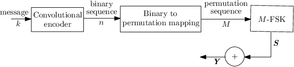
Refer to caption
Figure 1: System model for permutation trellis encoder.

Permutation trellis codes combine convolutional codes and permutation codes at the encoder and are decoded using a modified Viterbi decoder [ferreira-vinck-swart-beer]. A convolutional code is characterized by its rate RC=k/nR_{\text{C}}=k/n, the constraint length KK and the generator polynomial in an octal notation. The encoder uses K−kK-k shift registers and can be interpreted using a state transition diagram example shown in Fig. 1 having 2(K−k)2^{(K-k)} states. The octal generator notation is used to represent the XOR adder (output) connections of the inputs to the shift registers. As an example, an octal generator vector (7 5), having two elements represents a k=1k=1, n=2n=2 encoder which uses two (n=2n=2) XOR adders. There are one current input and two delayed inputs in the shift register. For the first adder (output), the binary vector of octal 7 is [1 1 1], while the binary vector of 5 is [1 0 1] for the second adder. A ‘1’ indicates a connection between an input or a delayed input in the shift register and the XOR adder of the encoder, while a ‘0’ indicates no connection to the adder.

The nn-tuple output from the convolutional encoder is uniquely mapped onto a codeword belonging to a permutation codebook 𝑪\boldsymbol{C}. The codebook 𝑪\boldsymbol{C} is a subset of all possible permutation of integers c1,c2,…​cMc_{1},c_{2},\dots c_{M}. All the codewords in 𝑪\boldsymbol{C} can be arranged in a matrix which consists of 2n2^{n} rows and each row contains a codeword 𝒄q\boldsymbol{c}_{q} at row qq (1≤q≤2n)(1\leq q\leq 2^{n}). Any two codewords 𝒄1,𝒄2\boldsymbol{c}_{1},\boldsymbol{c}_{2} have a Hamming distance dH​(𝒄1,𝒄2)d_{\text{H}}(\boldsymbol{c}_{1},\boldsymbol{c}_{2}) between them, which is the number of positions where the two codewords differ. The permutation codebook has a minimum Hamming distance dmind_{\text{min}}, which is the lowest Hamming distance between all possible, distinct codeword pairs. In mapping the convolutional codeword onto the permutation codeword, the combined code rate of PTC becomes RP=k/MR_{\text{P}}=k/M. The permutation codebook is chosen such that n≤Mn\leq M and the mapping is done such that the Hamming distance between each binary sequence and its respective permutation sequence is preserved, reduced or increased. Two examples of n=2n=2 mapped onto an M=3M=3 codebook and n=3n=3 mapped onto an M=4M=4 codebook are shown in Table 1. In Fig. 2(a), the state transition diagram of the n=2,M=3n=2,M=3 mapping is shown, where the non-binary sequence replaces the binary output of the convolutional encoder as an input bit (in brackets) produces an output and transition between states. The trellis representation of the code is shown in Fig. 2(b), where the dotted lines represent an input bit ‘1’, while the solid lines in the trellis represent an input bit ‘0’.

Table 1: Two sample mappings of binary outputs of convolutional code to non-binary permutation codes
nn = 2 MM=3 nn = 3 MM = 4
00 123 000 1234
01 132 001 1342
10 213 010 1423
11 231 011 2143
100 2314
101 2413
110 3241
111 3412

We refer the reader to other examples of distance increasing, reducing and preserving mappings in [ferreira-vinck, ferreira-vinck-swart-beer, chang-chen-klove-tsai].

Refer to caption
(a) State transition diagram.
Refer to caption
(b) Trellis representation of the PTC.
Figure 2: State transition diagram and equivalent trellis for RC=1/2R_{\text{C}}=1/2 and RP=1/3R_{\text{P}}=1/3.

2.2 MM-ary Frequency Shift Keying with PTC

Consider a set of MM orthogonal signals 𝒔1,𝒔2,…,𝒔M\boldsymbol{s}_{1},\boldsymbol{s}_{2},\dots,\boldsymbol{s}_{M}, each having one of the MM different frequency components and a low pass vector representation [proakis]

𝒔m\displaystyle\boldsymbol{s}_{m} =(0,…,0⏟m−1,Es,0,…,0⏟M−m)T.\displaystyle=(\underbrace{0,\dots,0}_{m-1},\sqrt{E_{s}},\underbrace{0,\dots,0}_{M-m})^{T}. (1)

The notation (⋅)T(\cdot)^{T} denotes the transpose operation and the symbol energy EsE_{s} is in the mm-th (m=1,2,…,Mm=1,2,\dots,M) position denoting the mm-th frequency. The vector 𝒄q\boldsymbol{c}_{q} is modulated by permuting the signal 𝒔m\boldsymbol{s}_{m}, MM times or over MM time slots. Each time slot corresponds to each integer in 𝒄q\boldsymbol{c}_{q} and the value of each integer indicates the position of the symbol energy. Hence, an MM-FSK modulated codeword is equivalent to a permutation matrix 𝑺=[si​j]∈{0,1}M×M\boldsymbol{S}=[s_{ij}]\in\{0,1\}^{M\times M} of the form

𝑺=[s11s12…s1​Ms21s22…s2​M⋮⋮⋱⋮sM​1sM​2…sM​M].\displaystyle\boldsymbol{S}=\left[\begin{array}[]{cccc}s_{11}&s_{12}&\dots&s_{1M}\\ s_{21}&s_{22}&\dots&s_{2M}\\ \vdots&\vdots&\ddots&\vdots\\ s_{M1}&s_{M2}&\dots&s_{MM}\end{array}\right]. (2)

The rows represent the MM available frequencies while the columns represent the time slots. At each time slot, the position (i,j)(i,j) is set to ‘1’ if the frequency is conveying information, while other positions at the same time slot are set to ‘0’.

Assuming perfect synchronization between the transmitter and receiver, for a transmitted coded matrix 𝑺\boldsymbol{S}, non-coherent detection over an AWGN and PLC channel are considered. In the PLC channel, NBI and IN are common noise sources [middleton]. While IN may affect some or all frequencies in a time slot, NBI may affect one of the MM frequencies over a period of time as illustrated in [ferreira-vinck-swart-beer]. In the time domain, IN in an indoor environment occurs in short bursts and lasts for a short period of time. As a result, the occurrence may affect successive information-carrying symbols. In the case of NBI, the noise takes a frequency selective nature in which a certain frequency is affected over a period of time. Due to the random occurrence and short burst nature of IN, its arrival rate γ\gamma in units per second is used to model the Poisson process. If each IN occurs at an average duration TnoiseT_{\text{noise}}, then an average of γ​Tnoise\gamma T_{\text{noise}} samples are affected by IN in 1 second (s) and 1−γ​Tnoise1-\gamma T_{\text{noise}} samples are not affected by IN. At the output of the channel, each received sample can be modelled as

yi​j={ej​ϕ​si​j+vG,AWGN,ej​ϕ​si​j+vG+vI⋅p,PLC.y_{ij}=\begin{cases}e^{j\phi}s_{ij}+v_{\text{G}},&\text{AWGN},\\ e^{j\phi}s_{ij}+v_{\text{G}}+v_{\text{I}}\cdot p,&\text{PLC}.\end{cases} (3)

The phase ϕ\phi is a random variable, distributed uniformly between 0 and 2​π2\pi, the noise sample vGv_{\text{G}} has the Gaussian distribution 𝒞​𝒩​(0,N02)\mathcal{C}\mathcal{N}(0,\frac{N_{0}}{2}) and vIv_{\text{I}} models the IN as a complex variable with distribution 𝒞​𝒩​(0,Ni)\mathcal{C}\mathcal{N}(0,N_{i}). The Poisson-distributed variable pp models the occurrence of the IN with an impulsive index A=N0/NiA=N_{0}/N_{i}, describing the power of the impulse noise NiN_{i} in terms of the Gaussian noise power N0N_{0}.

The received code matrix 𝒀=[yi​j]∈𝒞M×M\boldsymbol{Y}=[y_{ij}]\in\mathcal{C}^{M\times M} is demodulated by comparing each column vector in 𝒀\boldsymbol{Y} received from the output of the channel. Hence, for every transmitted vector 𝒔m\boldsymbol{s}_{m}, the received vector 𝒚\boldsymbol{y} (which forms a column in 𝒀\boldsymbol{Y}) is demodulated using ED by choosing the 𝒔m\boldsymbol{s}_{m} with the highest envelope

r=arg⁡maxm∈M​|𝒚H⋅𝒔m|.\displaystyle r=\displaystyle\arg\max_{m\in M}|\boldsymbol{y}^{H}\cdot\boldsymbol{s}_{m}|. (4)

This produces an integer rr which is equivalent to the likely transmitted mm-th frequency, hence a permutation of integers 𝒓=r1,r2,…,rM\boldsymbol{r}=r_{1},r_{2},\dots,r_{M} per transmitted codeword. A more adequate threshold detector proposed in [ferreira-vinck-swart-beer] sets a threshold of τ=0.6​Es\tau=0.6\sqrt{E_{s}} on the received samples, such that

ri​j={1,if ​y¯i​j≥τ,0,otherwise,r_{ij}=\begin{cases}1,&\text{if }\bar{y}_{ij}\geq\tau,\\ 0,&\text{otherwise},\end{cases} (5)

where y¯i​j=|yi​j|\bar{y}_{ij}=|y_{ij}|. This results in an M×MM\times M matrix 𝑹=[ri​j]∈{0,1}M×M\boldsymbol{R}=[r_{ij}]\in\{0,1\}^{M\times M}, equivalent to a transmitted signal 𝑺\boldsymbol{S}.

2.3 Probability of Error of PTC

Consider a set of transmitted code matrices 𝑺1,𝑺2,…,𝑺V\boldsymbol{S}^{1},\boldsymbol{S}^{2},\dots,\boldsymbol{S}^{V} which are received over an AWGN channel and demodulated as 𝑹1,𝑹2,…,𝑹V\boldsymbol{R}^{1},\boldsymbol{R}^{2},\dots,\boldsymbol{R}^{V}. For each transmitted code matrix 𝑺v\boldsymbol{S}^{v} (v=1,2,…,Vv=1,2,\dots,V), received and demodulated as 𝑹v\boldsymbol{R}^{v}, the probability of erroneously receiving the nn-tuple symbols encoded as 𝑺v\boldsymbol{S}^{v} is given as [bardan-masazade-ozdemir-varshney]

Pe=1M​∑i=12n∑v=12M2P⁡(𝑫=𝑺𝒗|𝑹v)⋅P⁡(𝑹v|𝑺=𝑺𝒗),P_{e}=\frac{1}{M}\sum^{2^{n}}_{i=1}\sum^{2^{M^{2}}}_{v=1}P(\boldsymbol{D}=\boldsymbol{S^{v}}|\boldsymbol{R}^{v})\cdot P(\boldsymbol{R}^{v}|\boldsymbol{S}=\boldsymbol{S^{v}}), (6)

where P⁡(𝑹v|𝑺=𝑺v)P(\boldsymbol{R}^{v}|\boldsymbol{S}=\boldsymbol{S}^{v}) is the likelihood of receiving 𝑹v\boldsymbol{R}^{v} if 𝑺v\boldsymbol{S}^{v} is transmitted and is given as

P⁡(𝑹v|𝑺=𝑺𝒗)=∏i=1M∏j=1M(∏w=1WP⁡(y¯i​j≥τ|si​j))​(∏u=1UP⁡(y¯i​j<τ|si​j)),P(\boldsymbol{R}^{v}|\boldsymbol{S}=\boldsymbol{S^{v}})=\prod_{i=1}^{M}\prod_{j=1}^{M}\left(\prod_{w=1}^{W}P(\bar{y}_{ij}\geq\tau|s_{ij})\right)\left(\prod_{u=1}^{U}P(\bar{y}_{ij}<\tau|s_{ij})\right), (7)

where UU and WW are the number of zeros (‘0’s) and ones (‘1’s) respectively in 𝑹v\boldsymbol{R}^{v}. P⁡(𝑫=𝑺𝒗|𝑹v)P(\boldsymbol{D}=\boldsymbol{S^{v}}|\boldsymbol{R}^{v}) is the probability of a correct decision because code matrix 𝑫\boldsymbol{D}, which has the minimum Hamming distance with the received code matrix 𝑹v\boldsymbol{R}^{v} is transmitted. The probabilities in (6) and (7), derived in [bardan-masazade-ozdemir-varshney, bardan-masazade-ozdemir-han-varshney] are given as

P⁡(y¯i​j≥τ|si​j=1)=Q1​(2​EsN0,0.6​2​EsN0),P(\bar{y}_{ij}\geq\tau|s_{ij}=1)=Q_{1}\left(\sqrt{2\frac{E_{s}}{N_{0}}},0.6\sqrt{2\frac{E_{s}}{N_{0}}}\right), (8)
P⁡(y¯i​j<τ|si​j=1)=1−P⁡(y¯i​j≥τ|si​j=1),P(\bar{y}_{ij}<\tau|s_{ij}=1)=1-P(\bar{y}_{ij}\geq\tau|s_{ij}=1), (9)
P⁡(y¯i​j≥τ|si​j=0)=exp​(−0.36​EsN0),P(\bar{y}_{ij}\geq\tau|s_{ij}=0)=\text{exp}\left(-0.36\frac{E_{s}}{N_{0}}\right), (10)

and

P⁡(y¯i​j<τ|si​j=0)=1−P⁡(y¯i​j≥τ|si​j=0).P(\bar{y}_{ij}<\tau|s_{ij}=0)=1-P(\bar{y}_{ij}\geq\tau|s_{ij}=0). (11)

Note that the SNR per symbol Es/N0E_{s}/N_{0} is the ratio of the received signal energy EsE_{s} to the noise power spectral density N0N_{0}, Q1​(α,β)=∫β∞x​exp​{−x2+α22}​I0​(α​x)​𝑑xQ_{1}(\alpha,\beta)=\int_{\beta}^{\infty}x\;\text{exp}\{-\frac{x^{2}+\alpha^{2}}{2}\}I_{0}(\alpha x)dx is the Marcum QQ-function [marcum] and I0​(α​x)I_{0}(\alpha x) is the zeroth order of the modified Bessel function. The PeP_{e} in (6), henceforth referred to as the analytical hard decision (HD) decoder gives the probability of error for a transmitted symbol nn. The convolutional code is an encoder with memory. Therefore, the decoder decodes the output of the demodulator as a chain of events whose length may not be fixed. In order to simplify the probability of error of the Viterbi decoder, the all-zero path is assumed to be transmitted. Therefore, the code’s free distance dfreed_{\text{free}}, which is the path which departs the all-zero path and first merges with the all-zero path is assumed to contain errors when compared with the transmitted all-zero path. As a result, the probability of error is bounded as [proakis, lin-costello]

Pe,CC≤∑d=dfree∞ad​P2​(d),P_{e,\text{CC}}\leq\sum_{d=d_{\text{free}}}^{\infty}a_{d}P_{2}(d), (12)

where P2​(d)P_{2}(d) describes the probability of the decoded path having a Hamming distance of dd bits with the transmitted codeword. When the binary convolutional code is mapped onto the non-binary permutation codeword, the Viterbi HD decoder’s Pe,C​CP_{e,CC} is modified as

Pe,CC𝒄≤∑d=dfree′∞ad𝒄P2𝒄(d),P_{e,\text{CC}}^{\boldsymbol{c}}\leq\sum_{d=d_{\text{free}}^{{}^{\prime}}}^{\infty}a_{d}^{\boldsymbol{c}}P_{2}^{\boldsymbol{c}}(d), (13)

where ad𝒄a_{d}^{\boldsymbol{c}} and P2𝒄​(d)P_{2}^{\boldsymbol{c}}(d) are similar to ada_{d} and P2​(d)P_{2}(d) in (12) but correspond to the permutation codeword 𝒄q\boldsymbol{c}_{q} mapped to a convolutional codeword and dfree′d_{\text{free}}^{{}^{\prime}} is the free distance of the non-binary code. Using the example mappings in Table 1, the all-zero sequence is equivalent to 123123 for M=3M=3 and 12341234 for M=4M=4. Hence, ad𝒄a_{d}^{\boldsymbol{c}} describes the paths with a Hamming distance of dd when compared with the transmitted permutation codeword equivalent to the corresponding all-zero codeword. If the path in error consists of VV stages, then a concatenation of matrices 𝑹1,𝑹2,…,𝑹V\boldsymbol{R}^{1},\boldsymbol{R}^{2},\dots,\boldsymbol{R}^{V} are received for transmitted code matrices 𝑺1,𝑺2,…,𝑺V\boldsymbol{S}^{1},\boldsymbol{S}^{2},\dots,\boldsymbol{S}^{V}. Therefore, the probability P2𝒄​(d)P_{2}^{\boldsymbol{c}}(d) is defined as

P2𝒄​(d)={∑dH​(𝑺v,𝑹v)=d2+1d∏v=1VP⁡(𝑹v|𝑺v), odd ​d,∑dH​(𝑺v,𝑹v)=d2+1d∏v=1VP⁡(𝑹v|𝑺v)+12​∏v=1VP⁡(𝑹v|𝑺v),even ​d,P_{2}^{\boldsymbol{c}}(d)=\begin{cases}\sum_{d_{\text{H}}(\boldsymbol{S}^{v},\boldsymbol{R}^{v})={\frac{d}{2}+1}}^{d}\prod_{v=1}^{V}P(\boldsymbol{R}^{v}|\boldsymbol{S}^{v}),\;\;\;\;\;\;\;\;\;\;\;\;\;\;\;\;\;\;\;\;\;\;\;\;\;\;\;\;\;\;\;\;\text{ odd }d,\\ \sum_{d_{\text{H}}(\boldsymbol{S}^{v},\boldsymbol{R}^{v})={\frac{d}{2}+1}}^{d}\prod_{v=1}^{V}P(\boldsymbol{R}^{v}|\boldsymbol{S}^{v})+\frac{1}{2}\prod_{v=1}^{V}P(\boldsymbol{R}^{v}|\boldsymbol{S}^{v}),\;\;\;\;\;\;\;\;\;\text{even }d,\\ \end{cases} (14)

where 𝑺v\boldsymbol{S}^{v} and 𝑹v\boldsymbol{R}^{v} are the transmitted and received matrices respectively at each stage vv in the trellis. At each stage of the trellis, the decoder computes the metric

dH​(𝑺v^,𝑹v)=M−(∑1≤i,j≤M(si​j∧ri​j)),\displaystyle d_{\text{H}}(\hat{\boldsymbol{S}^{v}},\boldsymbol{R}^{v})=M-(\sum_{1\leq i,j\leq M}(s_{ij}\land r_{ij})), (15)

between the received matrix 𝑹v\boldsymbol{R}^{v} and each branch 𝑺v^\hat{\boldsymbol{S}^{v}}. The decoder chooses the branch with the smallest metric, where the notation ∧\land is the binary AND operation. As a result, at each stage vv of the trellis, the probability of error P⁡(𝑹v|𝑺v)P(\boldsymbol{R}^{v}|\boldsymbol{S}^{v}) can be evaluated as pairwise, hence a function of the difference between 𝑹v\boldsymbol{R}^{v} and 𝑺v\boldsymbol{S}^{v} and is defined as

P⁡(𝑹v|𝑺v)=12​erfc​(RPM​EsN0​dH​(𝑺v,𝑹v)),P(\boldsymbol{R}^{v}|\boldsymbol{S}^{v})=\frac{1}{2}\text{erfc}\left(\sqrt{\frac{R_{\text{P}}}{M}\frac{E_{s}}{N_{0}}d_{\text{H}}(\boldsymbol{S}^{v},\boldsymbol{R}^{v})}\right), (16)

where erfc(xx) is the complementary error function of xx.

2.4 The Permutation Soft-Decision Decoder

As mentioned earlier, a permutation codeword of length MM permutes the MMFSK signal in (1), MM times. In each transmitted codeword matrix 𝑺\boldsymbol{S}, all MM frequencies carry information such that each frequency is activated once in each row and column. When the received signal is affected by AWGN or PLC channel noise, the PSDD solves the general assignment problem by minimizing

Zg=∑i=1M∑j=1My^i​j​si​j,Z_{g}=\sum_{i=1}^{M}\sum_{j=1}^{M}\hat{y}_{ij}s_{ij}, (17)

where y^i​j=−|yi​j|\hat{y}_{ij}=-|y_{ij}|, ZgZ_{g} is the cost at iteration gg and (17) is subject to

∑i=1Msi​j=∑j=1Msi​j=Es,\displaystyle\sum_{i=1}^{M}s_{ij}=\sum_{j=1}^{M}s_{ij}=\sqrt{E_{s}}, (18)

for i=1,2,…,Mi=1,2,\dots,M, j=1,2,…,Mj=1,2,\dots,M. The Hungarian algorithm (HA) [kuhn] can find the matrix 𝑺=[si​j]\boldsymbol{S}=[s_{ij}] that produces the minimum cost Z1Z_{1} with a corresponding row-column representation of the permutation sequence

{(1,j1),(2,j2),…,(M,jM)},{\{(1,j_{1}),(2,j_{2}),\dots,(M,j_{M})}\}, (19)

where j1,j2,…,jMj_{1},j_{2},\dots,j_{M} is a permutation of integers 1,2,…,M1,2,\dots,M. If the codeword corresponding to cost Z1Z_{1} produces a codeword 𝒄∉𝑪\boldsymbol{c}\notin\boldsymbol{C}, then the PSDD proceeds to the next iteration g=2g=2. Using Murty’s algorithm [murty], the PSDD ranks Z2,Z3,…,Z2nZ_{2},Z_{3},\dots,Z_{2^{n}} in order to find a codeword 𝒄∈𝑪\boldsymbol{c}\in\boldsymbol{C}. Using the solution matrix from Z1Z_{1}, n−1n-1 non-empty subsets of 𝒀\boldsymbol{Y} form nodes N1,N2,…,Nn−1N_{1},N_{2},\dots,N_{n-1}, by partitioning a1a_{1}. Nodes in this case are defined as

N1={(1,j1)¯},\displaystyle N_{1}={\{\overline{(1,j_{1})}}\},
N2={(1,j1),(OPEN2,j2)¯},\displaystyle N_{2}={\{(1,j_{1}),(\overline{2,j_{2})}}\},
⋮\displaystyle\vdots (20)
Nn−1={(1,j1),…,(n−1,jn−1)¯}.\displaystyle N_{n-1}={\{(1,j_{1}),\dots,\overline{(n-1,j_{n-1})}}\}.

Row-column pairs with the bar (⋅,⋅¯\overline{\cdot,\cdot}) indicate row-column elements to be replaced with ∞\infty while row-column elements without the bar are removed from 𝒀\boldsymbol{Y}. The minimum cost is then solved for each node and the node with the least cost forms the next assignment a2a_{2}.

The PSDD makes an optimal decision (OD) by using a brute force method to find the codeword 𝒄\boldsymbol{c} having the highest cost among all possible permutations

ZOD=arg⁡min𝒄q∈C​∑i=1M∑j=1My^i​j​si​j(𝒄q),for​ 1≤q≤2n,Z_{\text{OD}}=\arg\min_{\boldsymbol{c}_{q}\in C}\sum_{i=1}^{M}\sum_{j=1}^{M}\hat{y}_{ij}s^{(\boldsymbol{c}_{q})}_{ij},\quad\mbox{for}\ 1\leq q\leq 2^{n}, (21)

where si​j(𝒄q)s^{(\boldsymbol{c}_{q})}_{ij} is each element in the permutation matrix produced by a codeword 𝒄\boldsymbol{c}.

3 Proposed Soft-Decision Decoder and Schemes

3.1 Branch and Bound

In order to solve 𝒀\boldsymbol{Y} using BB, a set of M+1M+1 levels ϵ=0,1,2,…,M\epsilon=0,1,2,\dots,M are created and at each level ϵ>0\epsilon>0, there exists nodes t=1,2,…,M−ϵ+1t=1,2,\dots,M-\epsilon+1 each with cost δϵ(t)=δϵ(1),δϵ(2),…,δϵ(M−ϵ+1)\delta_{\epsilon}^{(t)}=\delta_{\epsilon}^{(1)},\delta_{\epsilon}^{(2)},\dots,\delta_{\epsilon}^{(M-\epsilon+1)} respectively. At ϵ=0\epsilon=0, there exists an initial node containing all integers {c1,c2,…,cM}\{c_{1},c_{2},\dots,c_{M}\} in no specific order and none of the MM jobs is yet assigned. An example of BB as an SD technique to solve an assignment problem is shown using a state space tree in Fig. 3 with M=4M=4. For simplicity, the initial node for M=4M=4 is 12341234 and nodes 1/2341/234, 2/1342/134 up to 4/1234/123 are obtained at ϵ=1\epsilon=1. The node tt with the minimum cost δ^ϵ(t)\hat{\delta}^{(t)}_{\epsilon} at ϵ=1\epsilon=1 with the minimum value from the MM branches is scheduled if

Refer to caption
Figure 3: Tree-based method to decode permutation codes using branch and bound with M=4M=4.
δ^ϵ(t)=min1≤t≤M⁡(y^ϵ​t+∑i,jy^i​j),ϵ=1,2≤i≤M,0<j≤M:j≠t.\hat{\delta}_{\epsilon}^{(t)}=\min_{1\leq t\leq M}(\hat{y}_{\epsilon t}+\sum_{i,j}\hat{y}_{ij}),\>\>\>\;\;\;\;\epsilon=1,2\leq i\leq M,0<j\leq M:j\neq t. (22)

The other nodes are pruned while the surviving node t^ϵ\hat{t}_{\epsilon} at ϵ=1\epsilon=1 satisfying (22) is divided into M−ϵM-\epsilon branches at the next level. At nodes ϵ>1\epsilon>1, the surviving node at each level

δ^ϵ(t)=min1≤t≤M⁡(y^(ϵ−1)​t^(ϵ−1)+y^ϵ​t+∑i,jy^i​j),ϵ>1,ϵ+1≤i≤M,1≤j≤M:j≠t,j∉𝒕^,\hat{\delta}_{\epsilon}^{(t)}=\min_{1\leq t\leq M}(\hat{y}_{(\epsilon-1)\hat{t}_{(\epsilon-1)}}+\hat{y}_{\epsilon t}+\sum_{i,j}\hat{y}_{ij}),\>\>\>\;\;\;\;\epsilon>1,\epsilon+1\leq i\leq M,1\leq j\leq M:j\neq t,j\notin\boldsymbol{\hat{t}}, (23)

where 𝒕^\boldsymbol{\hat{t}} contains an ordered set of scheduled nodes. This process of pruning and branching is done until the last level at which only one assignment is possible.

3.2 Schemes

As shown in Fig. 4, the PSDD uses BB or HA and Murty algorithms to decode 𝒀\boldsymbol{Y}, hence the dashed lines. The dotted lines around the Murty block indicates the Murty algorithm is only used when 𝒄∉𝑪\boldsymbol{c}\notin\boldsymbol{C} at HA. Otherwise, the Murty step is skipped.

3.2.1 Scheme 1

The channel output 𝒀\boldsymbol{Y} is decoded using HA (g=1g=1) and Murty (2≤g≤M2\leq g\leq M). The codeword matrix which maximizes (17) is then decoded using the Viterbi decoder. If HA produces a sequence 𝒄∉𝑪\boldsymbol{c}\notin\boldsymbol{C}, Murty iterates until 𝒄∈𝑪\boldsymbol{c}\in\boldsymbol{C} or the specified maximum number of iterations is reached.
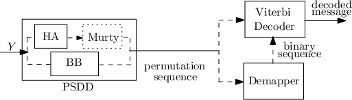
Refer to caption
Figure 4: Decoder system model of permutation code soft-decision and permutation trellis decoder.

3.2.2 Scheme 2

Here, the Viterbi decoder is used to decode the binary output from the permutation to binary code demapper. The PSDD produces a permutation code 𝒄\boldsymbol{c} that is demapped to its binary equivalent. If the final iteration of the PSDD produces a codeword 𝒄∉𝑪\boldsymbol{c}\notin\boldsymbol{C}, minimum distance decoding between 𝒄\boldsymbol{c} and all codewords in 𝑪\boldsymbol{C} is performed before demapping. This binary output is then decoded using the Viterbi decoder.

3.2.3 Schemes 3 & 4

In Scheme 3, the channel output 𝒀\boldsymbol{Y} or demodulated 𝒀¯\bar{\boldsymbol{Y}} is decoded with BB to solve for Z1Z_{1}. The permutation sequence produced is then forwarded to the Viterbi decoder. In Scheme 4, the permutation sequence produced by BB is demapped to its binary equivalent and forwarded to the Viterbi decoder, similar to Scheme 2. BB uses a single iteration, hence only Z1Z_{1} is solved in Schemes 3 and 4.

In the case where the threshold detector is used at the demodulator, the SD algorithms can also be applied to demodulated bits. As an example, consider a transmitted codeword 3214. The demodulated codeword matrix 𝒀¯I\bar{\boldsymbol{Y}}_{\text{I}} affected by impulse noise at time t4t_{4} can be represented as

𝒀¯I=
 

t1t2t3t40011010110010001​

 
 or 
𝒀¯N=t1t2t3t41111f10100f21000f30001f4​,whenaffectedbyNBIatf_1.Y¯_IandY¯_NcanbeeasilysolvedusingthePSDDtoproducethecodeword3214asshownbytheboxedvalues.ThecodewordcanthenbedecodedusingtheViterbialgorithm. 4 section 4 4 §4 4Simulation Results and Complexity Analysis We compare the simulated BER of the PTC decoder with the BERs obtained from the proposed decoding schemes discussed in Section 3.2. The BER is calculated as the ratio between the difference between the transmitted message bits and decoded bits, and the total number of transmitted bits. This is evaluated over an AWGN and PLC channel. Different PTC mappings are simulated, with three different codes. The first code has a rate = R C / 1 2 mapped onto = M 3 , the second has a rate = R C / 2 3 mapped onto = M 4 codebook while the third is a distance preserving mapping from = R C / 1 4 onto an = M 4 codebook. The first is generated from = K 3 , with an octal generator polynomial (7 5) while the second is generated from = K 4 , with an octal generator polynomial (1 3 0; 3 2 3). The mappings of both codes have been shown in Table 1. The third code is generated from = R C / 1 4 , = K 6 , with an octal generator polynomial (53 67 71 75). The third code is mapped onto a distance preserving permutation codebook of = M 4 . The SNR per bit / E b N 0 of the system for bit energy E b is defined as (25) Equation 25 25 = E b N 0 E s × N 0 R P ⁢ log 2 M . = E b N 0 E s × N 0 R P ⁢ log 2 M . For the PLC channel, we adopt the heavily disturbed channel scenario in [ma-so-gunawan] where the inter arrival time is 0.0196 s while T noise is 0.0641 ms. Figure 5 Figure 5 5 Figure 5 5BER comparisons of HD with SD schemes for code having R C = 1/2 and M = 3. Figure 5BER comparisons of HD with SD schemes for code having R C = 1/2 and M = 3. Figure 6 Figure 6 6 Figure 6 (a) 6(a) 6(a) (a)Schemes 1 & 3 with Viterbi decoding of PTC codewords. (a)Schemes 1 & 3 with Viterbi decoding of PTC codewords. (b) 6(b) 6(b) (b)Schemes 2 & 4 with Viterbi decoding of demapped codewords. (b)Schemes 2 & 4 with Viterbi decoding of demapped codewords. 6BER comparing the four PSDD decoding schemes with the PTC decoder for R C = 1/2 and M = 3 in AWGN channel. Figure 6BER comparing the four PSDD decoding schemes with the PTC decoder for R C = 1/2 and M = 3 in AWGN channel. Figs. and show the performance of the SD schemes over the AWGN channel. The SD schemes are compared with the expressions in (14) - (16). The simulated HD plot matches the analytical plot at higher SNRs, while the SD decoders improve the coding gain by about 2 dB. The BB method in Scheme 3 shows a slightly poorer performance when compared with Scheme 1 at lower SNRs. Results in Figs. and show a tight BER performance between the modified PTC decoder and the SD schemes. The BER of the Viterbi decoder when the all-zero codeword is compared with the d free path, as described in (13) is also shown in and as the d free bound. This bound can be considered as a lower bound. When M is increased in Figs. and , the BER coding gains obtainable from Schemes 1 and 2 become more evident with up to 3 dB gain at = g 4 . Figs. and show significant coding gains in the PLC channel with Schemes 3 and 4 performing close to the OD of Schemes 1 and 2. 4.1 subsection 4.1 4.1 §4.1 4.1BER Performance and 2 n ! M ratio The SD decoders presented provide the advantage of always outputting a permutation of integers by solving an assignment problem. The SD decoder’s probability of producing a codeword ∈ c C can be described by the ratio 2 n ! M . Hence, the performance of the schemes approaches the OD performance as 2 n increases. For example, in the plots in Fig. , the 2 n unique binary sequences are mapped onto a codebook with = M 4 . Since = 2 n ! M 0.667 , each scheme of the SD decoders is more likely to choose a codeword ∈ c C . In Figs. and , more iterations such as = g 4 are required to produce ∈ c C compared to = g 1 . Schemes 2 and 4 further improve the performance of the SD because the demapping process chooses one of the 2 n possible binary sequences using Hamming distance decoding. In Schemes 1 and 3, the codeword matrix produced by the SD decoder likely belongs to ! M possible permutations, rather than the encoder’s 2 n codewords due to errors. Since < 2 n ! M , the probability of error of the schemes using demapping is lower, especially at lower SNRs. Figure 7 Figure 7 7 Figure 7 (a) 7(a) 7(a) (a)Schemes 1 & 3 with Viterbi decoding of PTC codewords. (a)Schemes 1 & 3 with Viterbi decoding of PTC codewords. (b) 7(b) 7(b) (b)Schemes 2 & 4 with Viterbi decoding of demapped codewords. (b)Schemes 2 & 4 with Viterbi decoding of demapped codewords. 7BER of PTC decoding for R C = 2/3, M = 4 and A = 0.1 in PLC channel. Figure 7BER of PTC decoding for R C = 2/3, M = 4 and A = 0.1 in PLC channel. Figure 8 Figure 8 8 Figure 8 (a) 8(a) 8(a) (a)Schemes 1 & 3 with Viterbi decoding of PTC codewords. (a)Schemes 1 & 3 with Viterbi decoding of PTC codewords. (b) 8(b) 8(b) (b)Schemes 2 & 4 with Viterbi decoding of demapped codewords. (b)Schemes 2 & 4 with Viterbi decoding of demapped codewords. 8BER of PTC decoding for R C = 1/4, M = 4 and A = 0.1 in PLC channel. Figure 8BER of PTC decoding for R C = 1/4, M = 4 and A = 0.1 in PLC channel. 4.2 subsection 4.2 4.2 §4.2 4.2Complexity Analysis In order to analyze the different complexities of the decoder, operations required to process the digital signal are considered. The complexity of the circuitry required for the processing is not considered in this work. For each received, coded signal at the output of the channel, the TD demodulates each received sample of the × M M code matrix. This requires a complexity of O ( M 2 ) to decide if each sample in the × M M matrix is above or below the threshold. The demodulated × M M matrix is further compared with the codebook, to find the codeword having the minimum Hamming distance. This step will compare all the 2 n codewords with the demodulated matrix, having M 2 elements. This requires a complexity of O ( ⋅ 2 n M 2 ) . For the PSDD, the complexity of the iterative decoder in Scheme 1 and 2 is O ( M 3 ) [liu-shell] at = g 1 and O ( M 4 ) [cox-miller-danchick-newnam] for 2 ≤ g ≤ M . When > g 1 , the complexities sum up, hence a worst case complexity of O ( M 4 ) . At each level of the tree-based BB method in Fig 3 and (22), M different computations are required on all the M nodes in order to find the minimum cost at each level. Since the number of nodes to process reduce at each level, the worst case complexity is considered and can be approximated as O ( ⁢ M 3 log M ) [lageweg-lenstra-rinnooy-kan]. Schemes 2 and 4 require a lookup process to demap to the binary equivalent at a complexity of O ( ⁢ M log M ) . 5 section 5 5 §5 5Conclusion The design of four decoding schemes, which combine three optimization algorithms to improve the BER performance of the PTC decoder is presented. The complexities of the different components of the decoding schemes are also analyzed. Demapping the permutation sequence to its binary equivalent before decoding with the Viterbi decoder produces the best BER coding gain when compared to the PTC decoder. The BER coding gains obtained from the schemes increase as the ratio of the permutation codebook’s cardinality to all possible permutations increases. While the improved BER coding gain is at the expense of additional complexity, a reasonable trade-off can be considered when the permutation codebook contains large codewords. While multi-tone M -FSK has been established to improve the data rate of the M -FSK scheme, future work will require techniques for increasing the data rate of permutation-coded M -FSK. Acknowledgement The authors would like to thank and acknowledge the financial support provided by South Africa’s National Research Foundation (112248 & 114626) and the Sibanye-Stillwater Digital Mining Laboratory (DigiMine), Wits Mining Institute (WMI), University of the Witwatersrand, Johannesburg, South Africa. References 1 [1] ferreira-vinck H. C. Ferreira, A. J. H. Vinck, Interference cancellation with permutation trellis codes, in: Vehicular Technology Conference Fall 2000. IEEE VTS Fall VTC2000. 52nd Vehicular Technology Conference (Cat. No.00CH37152), Vol. 5, 2000, pp. 2401–2407 vol.5 (Sep. 2000). doi:10.1109/VETECF.2000.883295. 2 [2] ferreira-vinck-swart-beer H. C. Ferreira, A. J. H. Vinck, T. G. Swart, I. de Beer, Permutation trellis codes, IEEE Transactions on Communications 53 (11) (2005) 1782–1789 (Nov. 2005). doi:10.1109/TCOMM.2005.858683. 3 [3] vinck A. J. H. Vinck, Coding for a terrible channel, in: EU-COST289 2nd Workshop Special Topics on 4G Technologies, University of Duisburg-Essen, Germany, Jul. 8-9, 2005, pp. 101–106 (Jul. 8-9, 2005). 4 [4] lukusa-ouahada-ferreira T. Lukusa, K. Ouahada, H. C. Ferreira, Mathematical approach and implementation of frequency mapping techniques in power-line communications channel, Communications in Applied and Industrial Mathematics 10 (1) (2019) 88 – 108 (2019). URL https://content.sciendo.com/view/journals/caim/10/1/article-p88.xml 5 [5] bardan-masazade-ozdemir-varshney R. E. Bardan, E. Masazade, O. Ozdemir, P. K. Varshney, Performance of permutation trellis codes in cognitive radio networks, in: 2012 35th IEEE Sarnoff Symposium, 2012, pp. 1–6 (2012). 6 [6] bardan-masazade-ozdemir-han-varshney R. El-Bardan, E. Masazade, O. Ozdemir, Y. S. Han, P. K. Varshney, Permutation trellis coded multi-level FSK signaling to mitigate primary user interference in cognitive radio networks, IEEE Transactions on Communications 64 (1) (2016) 104–116 (Jan 2016). doi:10.1109/TCOMM.2015.2504508. 7 [7] gagnon-haccoun F. Gagnon, D. Haccoun, Coding and modulation schemes for slow fading channels, IEEE Transactions on Communications 43 (2/3/4) (1995) 858–868 (Feb 1995). doi:10.1109/26.380118. 8 [8] ouahada K. Ouahada, Nonbinary convolutional codes and modified m-fsk detectors for power-line communications channel, Journal of Communications and Networks 16 (3) (2014) 270–279 (2014). 9 [9] chang-chen-klove-tsai J.-C. Chang, R.-J. Chen, T. Klove, S.-C. Tsai, Distance-preserving mappings from binary vectors to permutations, IEEE Transactions on Information Theory 49 (4) (2003) 1054–1059 (April 2003). doi:10.1109/TIT.2003.809507. 10 [10] proakis J. G. Proakis, M. Salehi, Digital Communications, 5th Edition, McGraw-Hill, 2008, Ch. 4,8, pp. 215–217, 491–525 (2008). 11 [11] kolade-versfeld-van-wyk O. Kolade, J. Versfeld, M. van Wyk, Soft-Decision decoding of permutation block codes in AWGN and Rayleigh fading channels, IEEE Communications Letters 21 (12) (2017) 2590–2593 (Dec 2017). doi:10.1109/LCOMM.2017.2745545. 12 [12] viterbi A. Viterbi, Error bounds for convolutional codes and an asymptotically optimum decoding algorithm, IEEE Transactions on Information Theory 13 (2) (1967) 260–269 (April 1967). doi:10.1109/TIT.1967.1054010. 13 [13] little-murty-sweeney-karel J. D. C. Little, K. G. Murty, D. W. Sweeney, C. Karel, An algorithm for the traveling salesman problem., Operations Research 11 (6) (1963) 972–989 (March 1963). 14 [14] ross-soland Ross, G. Terry, Soland, R. M., A branch and bound algorithm for the generalized assignment problem, Mathematical Programming 8 (1975) 91–103 (1975). doi:10.1007/BF01580430. URL https://doi.org/10.1007/BF01580430 15 [15] middleton D. Middleton, Statistical-physical model of electromagnetic interference, IEEE Transactions on Electromagnetic Compatibility EMC-19 (3) (1977) 106–127 (Aug 1977). 16 [16] marcum J. Marcum, Table of q functions., Rand Corporation (1950). 17 [17] lin-costello S. Lin, D. J. Costello, Error Control Coding, Second Edition, Prentice-Hall, Inc., Upper Saddle River, NJ, USA, 2004 (2004). 18 [18] kuhn H. W. Kuhn, The Hungarian method for the assignment problem, Naval Research Logistics Quarterly 2 (1-2) (1955) 83–97 (1955). doi:10.1002/nav.3800020109. URL http://dx.doi.org/10.1002/nav.3800020109 19 [19] murty K. Murty, Letter to the editor — an algorithm for ranking all the assignments in order of increasing cost, Operations Research 16 (3) (1968) 682–687 (1968). doi:10.1287/opre.16.3.682. URL http://dx.doi.org/10.1287/opre.16.3.682 20 [20] ma-so-gunawan Y. H. Ma, P. L. So, E. Gunawan, Performance analysis of OFDM systems for broadband power line communications under impulsive noise and multipath effects, IEEE Transactions on Power Delivery 20 (2) (2005) 674–682 (2005). 21 [21] liu-shell L. Liu, D. A. Shell, Assessing optimal assignment under uncertainty: An interval-based algorithm, The International Journal of Robotics Research 30 (7) (2011) 936–953 (2011). arXiv:https://doi.org/10.1177/0278364911404579, doi:10.1177/0278364911404579. URL https://doi.org/10.1177/0278364911404579 22 [22] cox-miller-danchick-newnam I. J. Cox, M. L. Miller, R. Danchick, G. E. Newnam, A comparison of two algorithms for determining ranked assignments with application to multitarget tracking and motion correspondence, IEEE Transactions on Aerospace and Electronic Systems 33 (1) (1997) 295–301 (Jan. 1997). doi:10.1109/7.570789. 23 [23] lageweg-lenstra-rinnooy-kan B. J. Lageweg, J. K. Lenstra, A. H. G. R. Kan, A general bounding scheme for the permutation flow-shop problem, Operations Research 26 (1) (1978) 53–67 (1978). URL http://0-www.jstor.org.innopac.wits.ac.za/stable/169891
\bar{\boldsymbol{Y}}_{\text{I}}=\scalebox{1.0}{\mbox{$\displaystyle\begin{array}[]{*{4}{c} l}t_{1}&t_{2}&t_{3}&t_{4}\\ 0&0&\framebox{1}&1\\ 0&\framebox{1}&0&1\\ \framebox{1}&0&0&1\\ 0&0&0&\framebox{1}\\ \end{array}$}}\text{ or }\bar{\boldsymbol{Y}}_{\text{N}}=\scalebox{1.0}{\mbox{$\displaystyle\begin{array}[]{*{4}{c} l}t_{1}&t_{2}&t_{3}&t_{4}&\\ 1&1&\framebox{1}&1&f_{1}\\ 0&\framebox{1}&0&0&f_{2}\\ \framebox{1}&0&0&0&f_{3}\\ 0&0&0&\framebox{1}&f_{4}\\ \end{array}$}},\end{equation}whenaffectedbyNBIat$f_1$.$\bar{\boldsymbol{Y}}_{\text{I}}$and$\bar{\boldsymbol{Y}}_{\text{N}}$canbeeasilysolvedusingthePSDDtoproducethecodeword3214asshownbytheboxedvalues.ThecodewordcanthenbedecodedusingtheViterbialgorithm.\par\par\lx@frontmatter@fallback\@@numbered@section{section}{toc}{Simulation Results and Complexity Analysis} We compare the simulated BER of the PTC decoder with the BERs obtained from the proposed decoding schemes discussed in Section \ref{sec:schemes}. The BER is calculated as the ratio between the difference between the transmitted message bits and decoded bits, and the total number of transmitted bits. This is evaluated over an AWGN and PLC channel. Different PTC mappings are simulated, with three different codes. The first code has a rate $R_{\text{C}}=1/2$ mapped onto $M=3$, the second has a rate $R_{\text{C}}=2/3$ mapped onto $M=4$ codebook while the third is a distance preserving mapping from $R_{\text{C}}=1/4$ onto an $M=4$ codebook. The first is generated from $K=3$, with an octal generator polynomial (7 5) while the second is generated from $K=4$, with an octal generator polynomial (1 3 0; 3 2 3). The mappings of both codes have been shown in Table \ref{table:binary-to-permutation-mapping}. The third code is generated from $R_{\text{C}}=1/4$, $K=6$, with an octal generator polynomial (53 67 71 75). The third code is mapped onto a distance preserving permutation codebook of $M=4$. The SNR per bit $E_{b}/N_{0}$ of the system for bit energy $E_{b}$ is defined as \begin{equation}\begin{aligned} \dfrac{E_{b}}{N_{0}}=\dfrac{E_{s}}{N_{0}\times R_{\text{P}}\times\text{log}_{2}{M}}.\end{aligned}\end{equation} For the PLC channel, we adopt the heavily disturbed channel scenario in \cite[cite]{[\@@bibref{Number}{ma-so-gunawan}{}{}]} where the inter arrival time is 0.0196 s while $T_{\text{noise}}$ is 0.0641 ms. \par\begin{figure}\centering\includegraphics[width]{diagrams/results/ptc_1_2_3_analytical_with_schemes.eps} \@@toccaption{{\lx@tag[ ]{{5}}{BER comparisons of HD with SD schemes for code having $R_{\text{C}}$ = 1/2 and $M$ = 3.}}}\@@caption{{\lx@tag[: ]{{\small Figure 5}}{\small BER comparisons of HD with SD schemes for code having $R_{\text{C}}$ = 1/2 and $M$ = 3.}}} \@add@centering\end{figure} \par\begin{figure}\begin{subfigure}[172.5pt]\centering\includegraphics[width]{diagrams/results/ptc_1_2_3_scheme_1_3.eps} \@@toccaption{{\lx@tag[ ]{{(a)}}{Schemes 1 \& 3 with Viterbi decoding of PTC codewords.}}}\@@caption{{\lx@tag[ ]{{\small(a)}}{\small Schemes 1 \& 3 with Viterbi decoding of PTC codewords.}}} \vskip 8.61108pt\@add@centering\end{subfigure}\begin{subfigure}[172.5pt]\centering\includegraphics[width]{diagrams/results/ptc_1_2_3_scheme_2_4.eps} \@@toccaption{{\lx@tag[ ]{{(b)}}{Schemes 2 \& 4 with Viterbi decoding of demapped codewords.}}}\@@caption{{\lx@tag[ ]{{\small(b)}}{\small Schemes 2 \& 4 with Viterbi decoding of demapped codewords.}}} \vskip 8.61108pt\@add@centering\end{subfigure}\@@toccaption{{\lx@tag[ ]{{6}}{BER comparing the four PSDD decoding schemes with the PTC decoder for $R_{\text{C}}$ = 1/2 and $M$ = 3 in AWGN channel.}}}\@@caption{{\lx@tag[: ]{{\small Figure 6}}{\small BER comparing the four PSDD decoding schemes with the PTC decoder for $R_{\text{C}}$ = 1/2 and $M$ = 3 in AWGN channel.}}} \end{figure} \par Figs. \ref{fig:ptc-awgn-analytical-schems} and \ref{fig:half-rate-awgn} show the performance of the SD schemes over the AWGN channel. The SD schemes are compared with the expressions in (\ref{eq:definition-of-P2d}) - (\ref{eq:definition-of-P-r-t}). The simulated HD plot matches the analytical plot at higher SNRs, while the SD decoders improve the coding gain by about 2 dB. The BB method in Scheme 3 shows a slightly poorer performance when compared with Scheme 1 at lower SNRs. Results in Figs. \ref{fig:ptc-awgn-123} and \ref{fig:ptc-awgn-demapped-123} show a tight BER performance between the modified PTC decoder and the SD schemes. The BER of the Viterbi decoder when the all-zero codeword is compared with the $d_{\text{free}}$ path, as described in (\ref{eq:pe-ptc}) is also shown in \ref{fig:ptc-awgn-123} and \ref{fig:ptc-awgn-demapped-123} as the $d_{\text{free}}$ bound. This bound can be considered as a lower bound. When $M$ is increased in Figs. \ref{fig:ptc-awgn-234} and \ref{fig:ptc-awgn-demapped-234}, the BER coding gains obtainable from Schemes 1 and 2 become more evident with up to 3 dB gain at $g=4$. Figs. \ref{fig:ptc-plc-144} and \ref{fig:ptc-plc-demapped-144} show significant coding gains in the PLC channel with Schemes 3 and 4 performing close to the OD of Schemes 1 and 2. \par\par\lx@frontmatter@fallback\@@numbered@section{subsection}{toc}{BER Performance and $\frac{2^n}{M!}$ ratio} The SD decoders presented provide the advantage of always outputting a permutation of integers by solving an assignment problem. The SD decoder's probability of producing a codeword $\boldsymbol{c}\in\boldsymbol{C}$ can be described by the ratio $\frac{2^{n}}{M!}$. Hence, the performance of the schemes approaches the OD performance as $2^{n}$ increases. For example, in the plots in Fig. \ref{fig:one-quarter-rate-plc}, the $2^{n}$ unique binary sequences are mapped onto a codebook with $M=4$. Since $\frac{2^{n}}{M!}=0.667$, each scheme of the SD decoders is more likely to choose a codeword $\boldsymbol{c}\in\boldsymbol{C}$. In Figs. \ref{fig:half-rate-awgn} and \ref{fig:two-third-rate-awgn-iterations}, more iterations such as $g=4$ are required to produce $\boldsymbol{c}\in\boldsymbol{C}$ compared to $g=1$. Schemes 2 and 4 further improve the performance of the SD because the demapping process chooses one of the $2^{n}$ possible binary sequences using Hamming distance decoding. In Schemes 1 and 3, the codeword matrix produced by the SD decoder likely belongs to $M!$ possible permutations, rather than the encoder's $2^{n}$ codewords due to errors. Since $2^{n}<M!$, the probability of error of the schemes using demapping is lower, especially at lower SNRs. \par\begin{figure}\begin{subfigure}[172.5pt]\centering\includegraphics[width]{diagrams/results/ptc_2_3_4_scheme_1_3_plc.eps} \@@toccaption{{\lx@tag[ ]{{(a)}}{Schemes 1 \& 3 with Viterbi decoding of PTC codewords.}}}\@@caption{{\lx@tag[ ]{{\small(a)}}{\small Schemes 1 \& 3 with Viterbi decoding of PTC codewords.}}} \vskip 8.61108pt\@add@centering\end{subfigure}\begin{subfigure}[172.5pt]\centering\includegraphics[width]{diagrams/results/ptc_2_3_4_scheme_2_4_plc.eps} \@@toccaption{{\lx@tag[ ]{{(b)}}{Schemes 2 \& 4 with Viterbi decoding of demapped codewords.}}}\@@caption{{\lx@tag[ ]{{\small(b)}}{\small Schemes 2 \& 4 with Viterbi decoding of demapped codewords.}}} \vskip 8.61108pt\@add@centering\end{subfigure}\@@toccaption{{\lx@tag[ ]{{7}}{BER of PTC decoding for $R_{\text{C}}$ = 2/3, $M$ = 4 and $A$ = 0.1 in PLC channel.}}}\@@caption{{\lx@tag[: ]{{\small Figure 7}}{\small BER of PTC decoding for $R_{\text{C}}$ = 2/3, $M$ = 4 and $A$ = 0.1 in PLC channel.}}} \end{figure} \par\begin{figure}\begin{subfigure}[172.5pt]\centering\includegraphics[width]{diagrams/results/ptc_1_4_4_scheme_1_3_plc.eps} \@@toccaption{{\lx@tag[ ]{{(a)}}{Schemes 1 \& 3 with Viterbi decoding of PTC codewords.}}}\@@caption{{\lx@tag[ ]{{\small(a)}}{\small Schemes 1 \& 3 with Viterbi decoding of PTC codewords.}}} \vskip 8.61108pt\@add@centering\end{subfigure}\begin{subfigure}[172.5pt]\centering\includegraphics[width]{diagrams/results/ptc_1_4_4_scheme_2_4_plc.eps} \@@toccaption{{\lx@tag[ ]{{(b)}}{Schemes 2 \& 4 with Viterbi decoding of demapped codewords.}}}\@@caption{{\lx@tag[ ]{{\small(b)}}{\small Schemes 2 \& 4 with Viterbi decoding of demapped codewords.}}} \vskip 8.61108pt\@add@centering\end{subfigure}\@@toccaption{{\lx@tag[ ]{{8}}{BER of PTC decoding for $R_{\text{C}}$ = 1/4, $M$ = 4 and $A$ = 0.1 in PLC channel.}}}\@@caption{{\lx@tag[: ]{{\small Figure 8}}{\small BER of PTC decoding for $R_{\text{C}}$ = 1/4, $M$ = 4 and $A$ = 0.1 in PLC channel.}}} \end{figure} \par\par\par\lx@frontmatter@fallback\@@numbered@section{subsection}{toc}{Complexity Analysis} In order to analyze the different complexities of the decoder, operations required to process the digital signal are considered. The complexity of the circuitry required for the processing is not considered in this work. For each received, coded signal at the output of the channel, the TD demodulates each received sample of the $M\times M$ code matrix. This requires a complexity of $O(M^{2})$ to decide if each sample in the $M\times M$ matrix is above or below the threshold. The demodulated $M\times M$ matrix is further compared with the codebook, to find the codeword having the minimum Hamming distance. This step will compare all the $2^{n}$ codewords with the demodulated matrix, having $M^{2}$ elements. This requires a complexity of $O(2^{n}\cdot M^{2})$. For the PSDD, the complexity of the iterative decoder in Scheme 1 and 2 is $O(M^{3})$ \cite[cite]{[\@@bibref{Number}{liu-shell}{}{}]} at $g=1$ and $O(M^{4})$ \cite[cite]{[\@@bibref{Number}{cox-miller-danchick-newnam}{}{}]} for $2\leq g\leq M$. When $g>1$, the complexities sum up, hence a worst case complexity of $O(M^{4})$. At each level of the tree-based BB method in Fig \ref{fig:branch-and-bound-tree-diagram} and (\ref{branch-and-bound-level-0}), $M$ different computations are required on all the $M$ nodes in order to find the minimum cost at each level. Since the number of nodes to process reduce at each level, the worst case complexity is considered and can be approximated as $O(M^{3}\text{log}M)$ \cite[cite]{[\@@bibref{Number}{lageweg-lenstra-rinnooy-kan}{}{}]}. Schemes 2 and 4 require a lookup process to demap to the binary equivalent at a complexity of $O(M\text{log}M)$. \par\par\par\par\par\lx@frontmatter@fallback\@@numbered@section{section}{toc}{Conclusion} The design of four decoding schemes, which combine three optimization algorithms to improve the BER performance of the PTC decoder is presented. The complexities of the different components of the decoding schemes are also analyzed. Demapping the permutation sequence to its binary equivalent before decoding with the Viterbi decoder produces the best BER coding gain when compared to the PTC decoder. The BER coding gains obtained from the schemes increase as the ratio of the permutation codebook's cardinality to all possible permutations increases. While the improved BER coding gain is at the expense of additional complexity, a reasonable trade-off can be considered when the permutation codebook contains large codewords. While multi-tone $M$-FSK has been established to improve the data rate of the $M$-FSK scheme, future work will require techniques for increasing the data rate of permutation-coded $M$-FSK. \par\par\lx@frontmatter@fallback\@@unnumbered@section{section}{Acknowledgement} The authors would like to thank and acknowledge the financial support provided by South Africa's National Research Foundation (112248 \& 114626) and the Sibanye-Stillwater Digital Mining Laboratory (DigiMine), Wits Mining Institute (WMI), University of the Witwatersrand, Johannesburg, South Africa. \par\par\thebibliography\reset@natbib@cites\@@lbibitem{ferreira-vinck}\NAT@@wrout{1}{}{}{}{[1]}{ferreira-vinck}\lx@bibnewblock H.\penalty\ C. {Ferreira}, A.\penalty\ J.\penalty\ H. Vinck, Interference cancellation with permutation trellis codes, in: Vehicular Technology Conference Fall 2000. IEEE VTS Fall VTC2000. 52nd Vehicular Technology Conference (Cat. No.00CH37152), Vol.\penalty\ 5, 2000, pp. 2401--2407 vol.5 (Sep. 2000). \lx@bibnewblock\hrefhttps://doi.org/10.1109/VETECF.2000.883295. \par\reset@natbib@cites\@@lbibitem{ferreira-vinck-swart-beer}\NAT@@wrout{2}{}{}{}{[2]}{ferreira-vinck-swart-beer}\lx@bibnewblock H.\penalty\ C. Ferreira, A.\penalty\ J.\penalty\ H. Vinck, T.\penalty\ G. Swart, I.\penalty\ de\penalty\ Beer, Permutation trellis codes, IEEE Transactions on Communications 53\penalty\ (11) (2005) 1782--1789 (Nov. 2005). \lx@bibnewblock\hrefhttps://doi.org/10.1109/TCOMM.2005.858683. \par\reset@natbib@cites\@@lbibitem{vinck}\NAT@@wrout{3}{}{}{}{[3]}{vinck}\lx@bibnewblock A.\penalty\ J.\penalty\ H. Vinck, Coding for a terrible channel, in: EU-COST289 2nd Workshop Special Topics on 4G Technologies, University of Duisburg-Essen, Germany, Jul. 8-9, 2005, pp. 101--106 (Jul. 8-9, 2005). \par\reset@natbib@cites\@@lbibitem{lukusa-ouahada-ferreira}\NAT@@wrout{4}{}{}{}{[4]}{lukusa-ouahada-ferreira}\lx@bibnewblock T.\penalty\ Lukusa, K.\penalty\ Ouahada, H.\penalty\ C. Ferreira, \hrefhttps://content.sciendo.com/view/journals/caim/10/1/article-p88.xml, Communications in Applied and Industrial Mathematics 10\penalty\ (1) (2019) 88 -- 108 (2019). \newline URL \url{https://content.sciendo.com/view/journals/caim/10/1/article-p88.xml} \par\reset@natbib@cites\@@lbibitem{bardan-masazade-ozdemir-varshney}\NAT@@wrout{5}{}{}{}{[5]}{bardan-masazade-ozdemir-varshney}\lx@bibnewblock R.\penalty\ E. {Bardan}, E.\penalty\ {Masazade}, O.\penalty\ {Ozdemir}, P.\penalty\ K. {Varshney}, Performance of permutation trellis codes in cognitive radio networks, in: 2012 35th IEEE Sarnoff Symposium, 2012, pp. 1--6 (2012). \par\reset@natbib@cites\@@lbibitem{bardan-masazade-ozdemir-han-varshney}\NAT@@wrout{6}{}{}{}{[6]}{bardan-masazade-ozdemir-han-varshney}\lx@bibnewblock R.\penalty\ El-Bardan, E.\penalty\ Masazade, O.\penalty\ Ozdemir, Y.\penalty\ S. Han, P.\penalty\ K. Varshney, Permutation trellis coded multi-level {FSK} signaling to mitigate primary user interference in cognitive radio networks, IEEE Transactions on Communications 64\penalty\ (1) (2016) 104--116 (Jan 2016). \lx@bibnewblock\hrefhttps://doi.org/10.1109/TCOMM.2015.2504508. \par\reset@natbib@cites\@@lbibitem{gagnon-haccoun}\NAT@@wrout{7}{}{}{}{[7]}{gagnon-haccoun}\lx@bibnewblock F.\penalty\ Gagnon, D.\penalty\ Haccoun, Coding and modulation schemes for slow fading channels, IEEE Transactions on Communications 43\penalty\ (2/3/4) (1995) 858--868 (Feb 1995). \lx@bibnewblock\hrefhttps://doi.org/10.1109/26.380118. \par\reset@natbib@cites\@@lbibitem{ouahada}\NAT@@wrout{8}{}{}{}{[8]}{ouahada}\lx@bibnewblock K.\penalty\ {Ouahada}, Nonbinary convolutional codes and modified m-fsk detectors for power-line communications channel, Journal of Communications and Networks 16\penalty\ (3) (2014) 270--279 (2014). \par\reset@natbib@cites\@@lbibitem{chang-chen-klove-tsai}\NAT@@wrout{9}{}{}{}{[9]}{chang-chen-klove-tsai}\lx@bibnewblock J.-C. Chang, R.-J. Chen, T.\penalty\ Klove, S.-C. Tsai, Distance-preserving mappings from binary vectors to permutations, IEEE Transactions on Information Theory 49\penalty\ (4) (2003) 1054--1059 (April 2003). \lx@bibnewblock\hrefhttps://doi.org/10.1109/TIT.2003.809507. \par\reset@natbib@cites\@@lbibitem{proakis}\NAT@@wrout{10}{}{}{}{[10]}{proakis}\lx@bibnewblock J.\penalty\ G. Proakis, M.\penalty\ Salehi, Digital Communications, 5th Edition, McGraw-Hill, 2008, Ch. 4,8, pp. 215--217, 491--525 (2008). \par\reset@natbib@cites\@@lbibitem{kolade-versfeld-van-wyk}\NAT@@wrout{11}{}{}{}{[11]}{kolade-versfeld-van-wyk}\lx@bibnewblock O.\penalty\ Kolade, J.\penalty\ Versfeld, M.\penalty\ van Wyk, {Soft-Decision} decoding of permutation block codes in {AWGN} and {Rayleigh} fading channels, IEEE Communications Letters 21\penalty\ (12) (2017) 2590--2593 (Dec 2017). \lx@bibnewblock\hrefhttps://doi.org/10.1109/LCOMM.2017.2745545. \par\reset@natbib@cites\@@lbibitem{viterbi}\NAT@@wrout{12}{}{}{}{[12]}{viterbi}\lx@bibnewblock A.\penalty\ {Viterbi}, Error bounds for convolutional codes and an asymptotically optimum decoding algorithm, IEEE Transactions on Information Theory 13\penalty\ (2) (1967) 260--269 (April 1967). \lx@bibnewblock\hrefhttps://doi.org/10.1109/TIT.1967.1054010. \par\reset@natbib@cites\@@lbibitem{little-murty-sweeney-karel}\NAT@@wrout{13}{}{}{}{[13]}{little-murty-sweeney-karel}\lx@bibnewblock J.\penalty\ D.\penalty\ C. Little, K.\penalty\ G. Murty, D.\penalty\ W. Sweeney, C.\penalty\ Karel, An algorithm for the traveling salesman problem., Operations Research 11\penalty\ (6) (1963) 972--989 (March 1963). \par\reset@natbib@cites\@@lbibitem{ross-soland}\NAT@@wrout{14}{}{}{}{[14]}{ross-soland}\lx@bibnewblock Ross, G.\penalty\ Terry, Soland, R.\penalty\ M., \hrefhttps://doi.org/10.1007/BF01580430, Mathematical Programming 8 (1975) 91--103 (1975). \lx@bibnewblock\hrefhttps://doi.org/10.1007/BF01580430. \newline URL \url{https://doi.org/10.1007/BF01580430} \par\reset@natbib@cites\@@lbibitem{middleton}\NAT@@wrout{15}{}{}{}{[15]}{middleton}\lx@bibnewblock D.\penalty\ Middleton, Statistical-physical model of electromagnetic interference, IEEE Transactions on Electromagnetic Compatibility EMC-19\penalty\ (3) (1977) 106\textendash 127 (Aug 1977). \par\reset@natbib@cites\@@lbibitem{marcum}\NAT@@wrout{16}{}{}{}{[16]}{marcum}\lx@bibnewblock J.\penalty\ Marcum, Table of q functions., Rand Corporation (1950). \par\reset@natbib@cites\@@lbibitem{lin-costello}\NAT@@wrout{17}{}{}{}{[17]}{lin-costello}\lx@bibnewblock S.\penalty\ Lin, D.\penalty\ J. Costello, Error Control Coding, Second Edition, Prentice-Hall, Inc., Upper Saddle River, NJ, USA, 2004 (2004). \par\reset@natbib@cites\@@lbibitem{kuhn}\NAT@@wrout{18}{}{}{}{[18]}{kuhn}\lx@bibnewblock H.\penalty\ W. Kuhn, \hrefhttp://dx.doi.org/10.1002/nav.3800020109, Naval Research Logistics Quarterly 2\penalty\ (1-2) (1955) 83--97 (1955). \lx@bibnewblock\hrefhttps://doi.org/10.1002/nav.3800020109. \newline URL \url{http://dx.doi.org/10.1002/nav.3800020109} \par\reset@natbib@cites\@@lbibitem{murty}\NAT@@wrout{19}{}{}{}{[19]}{murty}\lx@bibnewblock K.\penalty\ Murty, \hrefhttp://dx.doi.org/10.1287/opre.16.3.682, Operations Research 16\penalty\ (3) (1968) 682--687 (1968). \lx@bibnewblock\hrefhttps://doi.org/10.1287/opre.16.3.682. \newline URL \url{http://dx.doi.org/10.1287/opre.16.3.682} \par\reset@natbib@cites\@@lbibitem{ma-so-gunawan}\NAT@@wrout{20}{}{}{}{[20]}{ma-so-gunawan}\lx@bibnewblock Y.\penalty\ H. {Ma}, P.\penalty\ L. {So}, E.\penalty\ {Gunawan}, Performance analysis of {OFDM} systems for broadband power line communications under impulsive noise and multipath effects, IEEE Transactions on Power Delivery 20\penalty\ (2) (2005) 674--682 (2005). \par\reset@natbib@cites\@@lbibitem{liu-shell}\NAT@@wrout{21}{}{}{}{[21]}{liu-shell}\lx@bibnewblock L.\penalty\ Liu, D.\penalty\ A. Shell, \hrefhttps://doi.org/10.1177/0278364911404579, The International Journal of Robotics Research 30\penalty\ (7) (2011) 936--953 (2011). \lx@bibnewblock\hrefhttp://arxiv.org/abs/https://doi.org/10.1177/0278364911404579, \hrefhttps://doi.org/10.1177/0278364911404579. \newline URL \url{https://doi.org/10.1177/0278364911404579} \par\reset@natbib@cites\@@lbibitem{cox-miller-danchick-newnam}\NAT@@wrout{22}{}{}{}{[22]}{cox-miller-danchick-newnam}\lx@bibnewblock I.\penalty\ J. Cox, M.\penalty\ L. Miller, R.\penalty\ Danchick, G.\penalty\ E. Newnam, A comparison of two algorithms for determining ranked assignments with application to multitarget tracking and motion correspondence, IEEE Transactions on Aerospace and Electronic Systems 33\penalty\ (1) (1997) 295--301 (Jan. 1997). \lx@bibnewblock\hrefhttps://doi.org/10.1109/7.570789. \par\reset@natbib@cites\@@lbibitem{lageweg-lenstra-rinnooy-kan}\NAT@@wrout{23}{}{}{}{[23]}{lageweg-lenstra-rinnooy-kan}\lx@bibnewblock B.\penalty\ J. Lageweg, J.\penalty\ K. Lenstra, A.\penalty\ H. G.\penalty\ R. Kan, \hrefhttp://0-www.jstor.org.innopac.wits.ac.za/stable/169891, Operations Research 26\penalty\ (1) (1978) 53--67 (1978). \newline URL \url{http://0-www.jstor.org.innopac.wits.ac.za/stable/169891} \par\endthebibliography \par\lx@frontmatter@fallback\@add@PDF@RDFa@triples\par\end{document}