Sequential hypothesis testing in machine learning, and crude oil price jump size detection
Abstract
In this paper, we present a sequential hypothesis test for the detection of the distribution of jump size in Lévy processes. Infinitesimal generators for the corresponding log-likelihood ratios are presented and analyzed. Bounds for infinitesimal generators in terms of super-solutions and sub-solutions are computed. This is shown to be implementable in relation to various classification problems for a crude oil price data set. Machine and deep learning algorithms are implemented to extract a specific deterministic component from the data set, and the deterministic component is implemented to improve the Barndorff-Nielsen & Shephard model, a commonly used stochastic model for derivative and commodity market analysis.
Key Words: Lévy processes, Hypothesis test, Machine learning, Crude oil price, Barndorff-Nielsen & Shephard model.
1 Introduction
Various existing hedging algorithms and insurance risks depend on the underlying statistical model of the commodity market. Consequently, an improvement in the underlying model directly improves the hedging strategies and the understanding of insurance risks. In this paper, we develop a novel statistical methodology for the refinement of stochastic models using various machine and deep learning algorithms.
As availability of information to the public through alternative data sources increases, machine learning is necessary for adequate analysis. Currently, 97% of North American businesses are using machine learning capabilities to analyze and apply data sources to their trading platforms and analytic focused activities (see [28]). The advent of these technologies allows participants to train, test, and project models using data that have historically been inaccessible. “Any innovation that makes better use of data, and enables data scientists to combine disparate sources of data in a meaningful fashion, offers the potential to gain competitive advantage” (see [28]). Trading capabilities, scale, scope, and speeds have increased exponentially with advancements in applications of Artificial Intelligence and Algorithmic trading.
A commonly used stochastic model for derivative and commodity market analysis is the Barndorff-Nielsen & Shephard (BN-S) model (see [2, 3, 4, 5, 13, 16, 18]). In [23], the BN-S model is implemented to find an optimal hedging strategy for the oil commodity from the Bakken, a new region of oil extraction that is benefiting from fracking technology. In [27], the BN-S model is used in this way, in the presence of quantity risk for oil produced in that region. In the recent paper [22], a machine learning-based improvement of the BN-S model is proposed. It is shown that this refined BN-S model is more efficient and has fewer parameters than other models which are used in practice as improvements of the BN-S model. Machine learning-based techniques are implemented for extracting a deterministic component () out of processes that are usually considered to be completely stochastic. Equipped with the aforementioned , the obtained refined BN-S stochastic model can be implemented to incorporate long-range dependence without actually changing the model.
It is clear that the real challenge is to obtain an estimation of the value of the deterministic component for an empirical data set. In [22], a naïve way to find this value for crude oil price is proposed. The method proposed in that paper provides an algorithm to form a classification problem for the data set. After that, various machine and deep learning techniques are implemented for that classification problem.
The primary motivation for this paper is the fact that the refined BN-S model can be successfully implemented to the analysis of crude oil price. In addition, it seems reasonable that some parameters of the refined BN-S model can be estimated by using various machine/deep learning algorithms. Consequently, it opens up the scope of an abundance of financial applications of the model to the commodity markets. With this motivation, in this paper, we investigate the problem from the perspective of sequential hypothesis testing. As described in [25], a sequential test of a hypothesis means any statistical test that gives a specific rule, at any stage of the experiment, for making one of the three decisions: (1) to accept the null hypothesis , (2) to reject , (3) to continue the experiment by making additional observation. Sequential hypothesis testing has many applications (see [6, 7, 11, 12]). In the paper [8], the problem of testing four hypotheses on two streams of observations is examined. A minimization result is obtained for the sampling time subject to error probabilities for distinguishing sequentially a standard versus a drifted two-dimensional Brownian motion. This result is further generalized in [20], where the testing of four hypotheses on two streams of observations that are driven by Lévy processes is presented. Consequently, the results in [20] are applicable for sequential decision making on the state of two-sensor systems. In one case, each sensor receives a Lévy process with a drift term or no drift term. For the other case, each sensor receives data driven by Lévy processes with large or small jumps. In this paper we show that a sequential test of a hypothesis can be implemented in relation to various classification problems for an empirical data set. Subsequently, machine and deep learning algorithms can be implemented to extract a deterministic component from a financial data set.
The organization of the paper is as follows. In Section 2, a refined BN-S model with some of its properties is presented. In Section 3, we provide a general jump size detection analysis based on the sequential testing of hypotheses. In Section 4, an overview of the data set is provided, and then two procedures in the predictive classification problem are introduced. Numerical results are shown in Section 4.3, and finally, a brief conclusion is provided in Section 5.
2 A refined Barndorff-Nielsen & Shephard model
Many models in recent literature try to capture the stochastic behavior of time series. As an example, for the Barndorff-Nielsen & Shephard model (BN-S model), the stock or commodity with price on some filtered probability space is modeled by
| (2.1) |
| (2.2) |
| (2.3) |
where the parameters with and and is the risk free interest rate where a stock or commodity is traded up to a fixed horizon date . In the above model is a Brownian motion, and the process is a subordinator. Also and are assumed to be independent, and is assumed to be the usual augmentation of the filtration generated by the pair .
However, the results and theoretical framework are far from being satisfactory. The BN-S model does not incorporate the long-range dependence property. As such, the model fails significantly for a longer ranges of time. To incorporate long-range dependence, a class of superpositions of Ornstein-Uhlenbeck (OU)-type processes is constructed in literature in terms of integrals with respect to independently scattered random measures (see [2, 14]). With appropriate conditions, the resulting processes are incorporated with long-range dependence. A limiting procedure results in processes that are second-order self-similar with stationary increments. Other resulting limiting processes are stable and self-similar with stationary increments. However, it is statistically unappealing to fit a large number of OU processes, at least by any formal likelihood-based method. To address this issue, in [22] a new method is developed.
As proposed in [22], on some filtered probability space , is given by (2.1), where the dynamics of in (2.2) is given by
| (2.4) |
where and are two independent subordinators, and is a deterministic parameter. Machine learning algorithms can be implemented to determine the value of . The process in (2.4) is a subordinator that has greater intensity than the subordinator . Also, , and are assumed to be independent, and is assumed to be the usual augmentation of the filtration generated by .
In this case (2.3) will be given by
| (2.5) |
where, as before, is deterministic. It is worth noting that when , (2.4) reduces to (2.2). Similarly, when , (2.5) reduces to (2.3).
We conclude this section with some properties of this new model. Note that , where , is also a Lévy subordinator that is positively correlated with both and . Note that the solution of (2.5) can be explicitly written as
| (2.6) |
The integrated variance over the time period is given by , and a straight-forward calculation shows
| (2.7) |
where
| (2.8) |
We derive a general expression for the characteristic function of the conditional distribution of the log-asset price process appearing in the BN-S model given by equations (2.1), (2.4) and (2.5). For simplicity, we assume
As shown in [22], the advantages of the dynamics given by (2.1), (2.4), and (2.5) over the existing models are significant. The following theorem is proved in [22]. From this result, it is clear that as is constantly adjusted, for a fixed , the value of always has an upper limit. Consequently, never becomes very small, and thus long-range dependence is incorporated in the model.
Theorem 2.1.
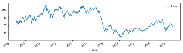
We implement the above analysis to empirical data sets. For example, we consider the West Texas Intermediate (WTI or NYMEX) crude oil prices data set for the period June 1, 2009 to May 30, 2019 (Figure 1). In the recent paper [22], the appropriateness of modeling such data with a BN-S type stochastic volatility model is discussed. It is clear that such a process is dependent on random shocks, and thus an implementation of the classical model is argued in [22]. However, in Figure 2, we provide the autocorrelation function of the given data set. It is clear that the long-range dependence criteria must be incorporated in the stochastic model. This justifies the implementation of the refined BN-S model presented in this section. We will discuss a detailed data analysis in Section 4. The implementation of the refined BN-S model in lieu of the classical BN-S model comes with the price of the estimation of as described earlier. In the later sections, this serves as a motivation to apply sequential hypothesis testing combined with various machine/deep learning algorithms. This leads to some novel numerical results related to the present data set.

We denote . Note that is also a subordinator. We call this the effective subordinator. We denote the cumulant transforms as . In this work, we make the following assumption similar to [19, 21].
Assumption 2.2.
Assume that .
We state the following well-known result from [19, 21] and denote the real part and imaginary part of as and , respectively.
Theorem 2.3.
Let be a subordinator with cumulant transform , and let be a complex-valued, left continuous function such that . Then
| (2.10) |
The above formula still holds if satisfies Assumption 2.2 and is such that , for .
The Laplace transform of , the conditional distribution of given the information up to time , is given by , for such that the expectation is well-defined.
Theorem 2.4.
In the case of the general BN-S model described in equations (2.1), (2.4) and (2.5), the Laplace transform of is given by
| (2.11) |
where .
The transform is well defined in the open strip , where
and
where .
Proof.
The proof is in the appendix. ∎
3 Jump size detection based on sequential hypothesis tests
In Section 2, it is observed that the refined BN-S model can be successfully implementable only when can be successfully computed for (2.4) and (2.5) (with ). Note that, as discussed in the previous section, the value of is in the interval . However, in order to simplify the subsequent analysis, is rounded to either or . This is motivated by the simplistic assumption that the jumps are either from one distribution or another. Also, in this case it is easier to interpret the confusion matrix corresponding to related classification algorithm. To find , in [22], a machine learning based empirical analysis is implemented. However, the procedure implemented in that paper does not incorporate any hypothesis testing for . In this section, we provide a more theoretical jump size detection analysis based on the sequential test of a hypothesis.
3.1 Theoretical results
We consider a Lévy process defined by Lévy triplet , where is the drift, is the diffusion, and for some Lévy measure defined on . We are interested in detecting a significant jump in the process. Consequently, we wish to test the hypotheses
| (3.1) |
which clearly address the size of the jumps in the Lévy process.
The Lévy process generates a filtration, which will be denoted , . Further, the hypotheses induce probability measures , . We seek to create a decision rule , where is a stopping rule with respect to , and is a random variable taking values in the index set , denoting which hypothesis to reject.
Let the log-likelihood ratio of the marginal density be given by
| (3.2) |
and consider an interval with . We define the decision rules to be
| (3.3) |
Theorem 3.1.
With the process defined as in (3.2), we have infinitesimal generators, given by
for any suitable , where
| (3.4) | ||||
| (3.5) | ||||
| (3.6) | ||||
| (3.7) |
Proof.
The proof is in the appendix. ∎
Assign to be the probability of a correct decision given . Then we have the partial integro-differential equations with boundary conditions
| (3.8) |
Further, we have inside .
Before proving the existence of a solution to the stated boundary value problem, we need a few more definitions and a theorem from [1] that will be used:
Definition 3.2.
An upper semicontinuous function is a subsolution of
subject to boundary conditions (3.8) if, for any test function , at each maximum point of in , we have
or
where
Similarly, a lower semicontinuous function is a supersolution of the same boundary value problem if for any test function , at each minimum point of in , we have
or
Finally, a viscosity solution is a function whose upper and lower semicontinuous envelopes are respectively a sub-solution and a super-solution.
Theorem 3.3.
If , and
- (A1)
if and ,
- (A2)
there exists such that for any
for some and as , we have
- (A3)
is uniformly continuous with respect to all arguments,
- (A4)
,
- (A5)
is a Lévy-Itô measure,
- (A6)
the inequalities in (3.9) are strict,
- (A7)
for any , there exists a modulus of continuity such that, for any , , , and for any satisfying
then there is a unique solution to between any pair of super-solution and sub-solutions, defined below, where
Lemma 3.4.
Proof.
The proof is in the appendix. ∎
It is known that if is a Lévy process then there exists a unique cádlág process such that
is called the stochastic exponential or Doléans-Dade exponential of and is denoted by . We now derive the infinitesimal generators. The results are motivated by [20]. Before proceeding, we present another formal definition:
Definition 3.5.
We write that a function if we have some satisfying for all . Similarly, we write that a function if for any , we have some satisfying for all .
The norm is defined as the essential supremum of the absolute value of over . It is the smallest number so that has measure zero.
Using all of the previous, we can finally state the existence theorem.
Theorem 3.6.
If is monotonic, then the partial integro-differential equation , subject to boundary conditions (3.8) and has a viscosity solution between sub-solution and super-solution
where
Proof.
The proof is in the appendix. ∎
Remark 3.7.
The existence of a more general viscosity solution to a higher dimensional problem is shown without assuming monotonicity in the paper [20]. The monotonicity assumption yields a tighter super- and sub-solution envelope and is here to make the application of this theorem to time series data more effective.
3.2 Jump size detection algorithm
We will use the prior super- and sub-solutions as envelopes to approximate an important parameter in the following algorithm that uses the previous hypothesis test to classify Lévy processes as having small or large jumps.
Given oil price close values in length- work day periods, we do the following:
- 1.
An inverse Gaussian density is fit to the distribution of negative percent daily jumps for the entire (training) data set.
- 2.
We then fit the density of the Lévy measure from 3.1, , to the distribution of the negative percent daily jumps for the -length period. This gives a test statistic for the parameter in the hypothesis test.
- 3.
We calculate the standard deviation of all daily percent changes for the -length period.
- 4.
- 5.
The left side of the interval is chosen to be , then using , , , , and in the super- and sub-solution equations in 3.6, we can solve for the right side of the interval using and , and take the average of the two. The parameter is chosen to be the maximum desired probability of a Type-I Error.
- 6.
Simulations of the log-likelihood process with drift , volatility , and jumps represented by an inverse Gaussian process with expected value at time , are run. We record the frequency of exits out of the right-side of the interval to get a number that represents, relatively, the size of the jumps. We call this number the right-exit frequency.
- 7.
Time periods whose right-exit frequencies are at or above a certain threshold are then classified as having large jumps, while the others are classified as having small jumps.
3.3 Effectiveness on simulated data
To demonstate the capacity of the hypothesis testing algorithm in distinguishing between processes with small and large jumps, we run it on simulated data. Multiple classes of Lévy processes are simulated, all of which start initially at :
- 1.
a training data time series with drift , diffusion , and jumps that follow an inverse Gaussian distribution with mean and scale factor , which gives a Lévy measure ,
- 2.
a control data set of processes with parameters identical to the training data,
- 3.
a data set of processes with obvious large negative jumps: the parameters are the same as the training set except the Lévy measure is now represented by , and
- 4.
a data set of processes with subtle large negative jumps: the drift is increased to compensate for the previous increase in jump size.
The training time series is run for time periods, and the other three are run for each, with representatives shown in Figure 3.
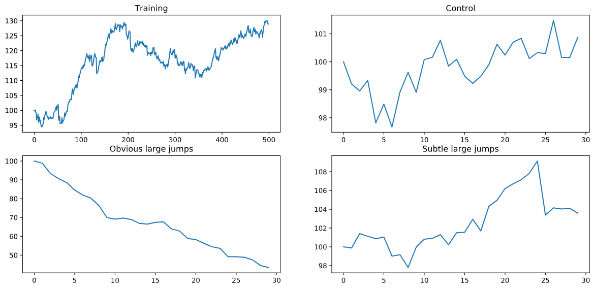
The hypothesis test algorithm with and is run on each data set. (The parameter is chosen here to gives desirable results and will be used in the application in the next section.) For the control, out of the processes are correctly identified as coming from the distribution with small jumps. This is to be expected because some number of processes would randomly have signficantly larger jumps just by chance. All from the obvious large jumps set are identified as having large jumps, and out of the processes in the subtle large jumps set are correctly identified.
Alternatively, a naïve approach of simply classifying each day period based on comparing only the mean jump size relative to the training data’s mean jump size results in only of the control processes being correctly identified; although it correctly identifies all but of the large jump simulations. Because of the significant potential for Type-I Error in this naïve approach, the hypothesis test algorithm has evident advantages.
4 Prediction method
We briefly discussed the data set in Section 2. In this section, we present an overview of the data set in its entirety, and then develop two procedures used in the predictive classification problem. As discussed in Section 2, we consider the West Texas Intermediate (WTI or NYMEX) crude oil prices data set for the period June 1, 2009 to May 30, 2019. West Texas Intermediate crude oil is described as light sweet oil traded and delivered at Cushing, Oklahoma. WTI usually refers to the price of the New York Mercantile Exchange (NYMEX) WTI Crude Oil futures contract. For WTI, spot and futures prices are used as a benchmark in oil pricing. The WTI crude oil futures contract specifies the deliverable asset for the contract to be a blend of crude oil, as long as it is of acceptable lightness and sweetness. The data set is available online in [29]. We index the available dates from 0 (for June 1, 2009) to 2529 (for May 30, 2019).
The following table (Table 1) summarizes various estimates for the data set.
| Daily Price Change | Daily Price Change % | |
|---|---|---|
| Mean | -0.0047 | 0.01370 % |
| Median | 0.04399 | 0.06521 % |
| Maximum | 7.62 | 12.32 % |
| Minimum | -8.90 | -10.53 % |
In Figure 4 the distribution plot for close oil price is provided. Histograms for daily change in close oil price and daily change percentage in close oil price are provided in Figure 5 and Figure 6, respectively, for exploratory purposes.


In the following subsections, two procedures are described for constructing the related classification problem. The procedures differ in the features used for the analysis: percent daily changes and right-exit frequencies. In each, the algorithm at the end of Section 3 is used to determine whether an individual time period has large or small jumps, represented by the right-exit frequency of that time period. The machine learning algorithms are then used to predict whether the right-exit frequency of the next time period will be large or small. Consequently, before truncation, the resulting probabilities of large jumps from each machine learning algorithm can be used to update from the refined BN-S model in Section 2 each period.
4.1 Percent daily changes as features
We implement the following procedure to create a machine learning classification problem:
- 1.
We consider the percent daily changes for the historical oil price data and create a new data-frame from the old where the columns will be consecutive daily change percents. For example, if the changes are
then the first row of the data set will be
and the second row will be
and so forth.
- 2.
We create a target column that is if the right-exit frequency of the next disjoint days is less than some threshold , and is otherwise. For example, if the time period
has a significant frequency of right-exits, then the time period
is given a target value .
- 3.
We run various classification algorithms where the input is a list of consecutive close prices, and the output is a to represent large jumps or to represent small jumps of the next consecutive close prices. Classification reports and confusion matrices are evaluated for each algorithm.
4.2 Right-exit frequencies as features
We implement the following procedure to create a machine learning classification problem:
- 1.
Similar to the previous, we consider close prices for the historical oil price data and create a new data-frame exactly as before.
- 2.
A new column is created that holds the right-exit frequencies for each consecutive set of days, say,
These represent how large the jumps in close prices are for the previous days.
- 3.
From this column, a new staggered data-frame is created, similar to before.
- 4.
Finally, a target column is created: if the row is
then the entry in the target column will be . This is the right-exit frequency of the next disjoint -day period.
- 5.
We run various classification algorithms where the input is a list of consecutive right-exit frequencies, and the output is to represent large jumps or to represent small jumps of the next consecutive close prices. Classification reports and confusion matrices are evaluated for each algorithm.
4.3 Numerical results
Now we apply the procedures described in the last section to specific cases. For this section, the period length . Further, , the parameter representing an approximation for the Type-I Error of the test is chosen to be , and because it worked optimally in the simulation study, the cut off for significant right-exit frequencies is chosen to be . Two different time periods are used for training, and two are used for testing. The time periods are
- •
: training data (index): October 21, 2009 (100) to May 17, 2013 (1000); and testing data (index): April 21, 2017 (2000) to April 10, 2019 (2500);
- •
: training data (index): August 11, 2009 (50) to May 13, 2013 (1500); and testing data (index): October 5, 2015 (1600) to January 29, 2019 (2450).
Because the data is significantly imbalanced in favor of small jump time periods, random small jump periods from the training data are removed while performing algorithms 4.1 and 4.2. This allows the neural nets and other algorithms to isolate the attributes of large and small jump periods without becoming distracted by the imbalanced frequency of small jump periods. Without doing so, the algorithms often predict all time periods to be small jump periods – simply because those are more prevalent. The results of the machine learning algorithms using the time periods above are recorded in the following tables (Tables 2-5). Those used are linear regression (LR), decision trees (DT), random forests (RF), and three different types of neural nets, (A) a standard net, (B) a long-short term memory net, and (C) a LSTM net with a batch normalizer.
Most of the machine learning algorithms perform better than how one might expect from guessing uniformly whether the next time period would have big jumps. Some perform notably poorly, however, particularly the LSTM neural nets without a batch normalizer. However, the neural nets with a batch normalizer consistently perform quite well.
Figure 7 provides a histogram showing the distribution of right-exit frequencies for period lengths of 30 business days in the testing data. For each set of 30 consecutive days, simulations are run, and the frequency of right-exits is recorded. The -axis in the figure is the number of simulated processes that exit to the right of the testing interval for a given period, while the -axis is the number of 30 day periods with that frequency of right-exits.
Once the value of is estimated, this can be implemented in the refined BN-S model (2.4) (and, (2.5), with ). Equipped with , as described in [22] and as shown in Theorem 2.1, the refined BN-S stochastic model can be used to incorporates long-range dependence without actually changing the model. In addition, this shows a real-time application of data science for extracting a deterministic component out of processes that are thus far considered to be completely stochastic. By the deterministic component, it is meant that is a deterministic signal. This is deterministic in the sense that its value is extracted from the data before the model is implemented. Once the value of is obtained, it is kept constant for a certain period of time. For the computational effectiveness of , the results in Tables 2-5 show better estimation compared to the benchmark study in [22].
| LR | DT | RF | Neural Network (A) | LSTM (B) | BN (C) | |
| precision | 0.92 | 0.89 | 0.89 | 0.88 | 0.83 | 0.93 |
| recall | 0.61 | 0.56 | 0.64 | 0.54 | 0.77 | 0.88 |
| f1-score | 0.74 | 0.69 | 0.74 | 0.67 | 0.80 | 0.90 |
| support | 340 | 340 | 340 | 340 | 340 | 340 |
| precision | 0.29 | 0.24 | 0.25 | 0.22 | 0.19 | 0.53 |
| recall | 0.76 | 0.67 | 0.60 | 0.64 | 0.26 | 0.66 |
| f1-score | 0.42 | 0.35 | 0.36 | 0.33 | 0.22 | 0.59 |
| support | 70 | 70 | 70 | 70 | 70 | 70 |
| LR | DT | RF | Neural Network (A) | LSTM (B) | BN (C) | |
| precision | 0.89 | 0.92 | 0.87 | 0.83 | 0.88 | 0.85 |
| recall | 0.66 | 0.67 | 0.69 | 0.56 | 0.21 | 0.71 |
| f1-score | 0.76 | 0.77 | 0.77 | 0.67 | 0.34 | 0.77 |
| support | 340 | 340 | 340 | 340 | 340 | 340 |
| precision | 0.24 | 0.30 | 0.25 | 0.17 | 0.18 | 0.21 |
| recall | 0.61 | 0.70 | 0.50 | 0.43 | 0.86 | 0.39 |
| f1-score | 0.37 | 0.42 | 0.33 | 0.24 | 0.30 | 0.27 |
| support | 70 | 70 | 70 | 70 | 70 | 70 |
| LR | DT | RF | Neural Network (A) | LSTM (B) | BN (C) | |
| precision | 0.79 | 0.74 | 0.79 | 0.80 | 0.77 | 0.75 |
| recall | 0.82 | 0.50 | 0.57 | 0.66 | 0.58 | 0.91 |
| f1-score | 0.80 | 0.59 | 0.66 | 0.72 | 0.66 | 0.82 |
| support | 519 | 519 | 519 | 519 | 519 | 519 |
| precision | 0.57 | 0.37 | 0.42 | 0.47 | 0.41 | 0.65 |
| recall | 0.53 | 0.63 | 0.68 | 0.63 | 0.63 | 0.37 |
| f1-score | 0.55 | 0.46 | 0.52 | 0.54 | 0.50 | 0.47 |
| support | 241 | 241 | 241 | 241 | 241 | 241 |
| LR | DT | RF | Neural Network (A) | LSTM (B) | BN (C) | |
| precision | 0.80 | 0.76 | 0.79 | 0.76 | 0.80 | 0.75 |
| recall | 0.54 | 0.56 | 0.58 | 0.54 | 0.16 | 0.63 |
| f1-score | 0.65 | 0.64 | 0.67 | 0.63 | 0.27 | 0.68 |
| support | 519 | 519 | 519 | 519 | 519 | 519 |
| precision | 0.42 | 0.39 | 0.42 | 0.39 | 0.34 | 0.40 |
| recall | 0.70 | 0.62 | 0.66 | 0.64 | 0.91 | 0.54 |
| f1-score | 0.52 | 0.48 | 0.52 | 0.49 | 0.49 | 0.46 |
| support | 241 | 241 | 241 | 241 | 241 | 241 |

5 Conclusion
Motivated by the fact that the refined BN-S model can be successfully implemented to the analysis of crude oil price, and that the parameters of the refined BN-S model can be estimated by using various machine/deep learning algorithms, in this paper we study the refined BN-S model from the sequential hypothesis testing perspective, with an application to the oil market.
Mathematical modeling of oil price data is directly inspired by various stochastic models. Thorough understanding and theoretical development of appropriate stochastic models contribute to a better understanding of the risk-management problem of various commodities, and various existing algorithms in a financial market depend on the underlying statistical model. Consequently, an improvement in the underlying model directly improves the existing algorithms. In this paper, a sequential decision making problem in connection to the Lévy process is studied to analyze the jump size distribution. This is coupled with various machine and deep learning techniques to improve the existing stochastic models. Consequently, the analysis presented in this paper provides a necessary mathematical framework for an appropriate generalization of various stochastic models.
Future works related to this topic should definitely include seeking to find a more adequate approximation for the right side of the decision rule interval. This would greatly increase the sensitivity of the algorithms in classifying large-jump time periods, thereby requiring less computational power for even better results. Applications to other data sets more independent of exogenous forces, and even across multiple streams of data using [20], should also be explored. Finally, constructing decision rules for hypothesis tests on other parameters in the underlying processes could open up this type of analysis to more generalized scenarios.
6 Appendix
Proof of Theorem 2.4:
Proof.
We obtain from equation (2.4)
where . Let denote the -algebra generated by up to time and by . Then, proceeding by iterated conditional expectations, we obtain
Using (2.7) we obtain
Clearly if , then . Thus the result follows from (2.10). ∎
Proof of Theorem 3.1:
Proof.
Since is a Lévy process with characteristics under and characteristics under , we apply the generalized Girsanov’s Theorem. Using as in (3.4), we obtain
where
is the jump measure for , is a standard Brownian motion, and is the Doléans-Dade exponential, defined below. This gives that is a Lévy process with characteristics
Then, by [10] (Proposition 8), we obtain characteristics
for . Finally, by [10, 17], the process has the stated generator.∎
Proof of Lemma 3.4:
Proof.
First, consider (A1):
if and .
Next, , so choosing , we have property (A2).
Property (A3) is satisfied because is linear in each argument, and (A4) is satisfied because does not depend on its first argument explicitly. Last, is a Lévy-Itô measure by the assumptions of the underlying Lévy process.
∎
Proof of Theorem 3.6:
Proof.
We define
Consequently,
can be rewritten as
The sign on is positive; therefore, we have sub-solution equation
On the other hand, since is monotonic and positive inside ,
Using this, we have super-solution equation
Finally, applying the previous theorem 3.3, we have the existence of a viscosity solution. ∎
Acknowledgment: The authors would like to thank the anonymous reviewers for their careful reading of the manuscript and for suggesting points to improve the quality of the paper.
References
- [1] G. Barles, E. Chasseigne, & C. Imbert (2008), On the Dirichlet Problem for Second-Order Elliptic Integro-Differential Equations, Indiana Univ. Math. J., 57 (1), 213-246.
- [2] O. E. Barndorff-Nielsen (2001), Superposition of Ornstein-Uhlenbeck Type Processes, Theory Probab. Appl., 45, 175-194.
- [3] O. E. Barndorff-Nielsen & N. Shephard (2001), Non-Gaussian Ornstein-Uhlenbeck-based models and some of their uses in financial economics, J. R. Stat. Soc. Ser. B Stat. Methodol., 63, 167-241.
- [4] O. E. Barndorff-Nielsen & N. Shephard (2001), Modelling by Lévy Processes for Financial Econometrics, In Lévy Processes : Theory and Applications (eds O. E. Barndorff-Nielsen, T. Mikosch & S. Resnick), 283-318, Birkhäuser.
- [5] O. E. Barndorff-Nielsen, J. L. Jensen & M. Srensen (1998), Some stationary processes in discrete and continuous time, Adv. in Appl. Probab., 30, 989-1007.
- [6] C. Baum & V. Veeravalli (1994), A sequential procedure for multihypothesis testing, IEEE Transactions on Information Theory, 40 (6), 1994-1997.
- [7] B. Brodsky & B. Darkhovsky (2008), Minimax methods for multihypothesis sequential testing and change-point detection problems, Sequential Analysis, 27 (2), 141-173.
- [8] M. Carlisle & O. Hadjiliadis (2013), Sequential Decision Making in Two-Dimensional Hypothesis Testing, 52nd IEEE Conference on Decision and Control, https://ieeexplore.ieee.org/document/6760919.
- [9] Y. S. Chow, H. Robbins, & D. Siegmund (1991), The theory of optimal stopping, Dover Publications.
- [10] R. Cont & P. Tankov (2003), Financial Modelling with Jump Processes, hapman and Hall/CRC Financial Mathematics Series.
- [11] S. Dayanik, V. Poor, & S. Sezer (2008), Sequential multi-hypothetis testing for compound Poisson processes, Stochastics, 80 (1), 19-50.
- [12] G. K. Golubev & R.Z. Khas’minski (1983), Sequential testing for several signals in Gaussian white noise, Theory of Probability and its applications, 28, 573-584.
- [13] S. Habtemicael & I. SenGupta (2016), Pricing variance and volatility swaps for Barndorff-Nielsen and Shephard process driven financial markets, International Journal of Financial Engineering, 03 (04), 1650027 (35 pages).
- [14] S. Habtemicael, M. Ghebremichael & I. SenGupta (2019), Volatility and variance swap using superposition of the Barndorff-Nielsen and Shephard type Lévy processes, Sankhya B, 81, 75-92.
- [15] A. Irle (1981), Transitivity in problems of optimal stopping, Annals of Probability, 9, 642-647.
- [16] A. Issaka & I. SenGupta (2017), Analysis of variance based instruments for Ornstein–Uhlenbeck type models: swap and price index, Annals of Finance, 13(4), 401-434.
- [17] G. Lowther (2010), Lévy Processes, Stochastic Calculus Notes , https://almostsure.wordpress.com/2010/11/23/levy-processes/.
- [18] T. Miljkovic & I. SenGupta (2018), A new analysis of VIX using mixture of regressions: examination and short-term forecasting for the S&P 500 market, High Frequency, 1 (1), 53-65.
- [19] E. Nicolato & E. Venardos (2003), Option Pricing in Stochastic Volatility Models of the Ornstein-Uhlenbeck type, Math. Finance, 13, 445-466.
- [20] M. Roberts & I. SenGupta (2020), Infinitesimal generators for two-dimensional Lévy process-driven hypothesis testing, Annals of Finance, 16 (1), 121-139.
- [21] I. SenGupta (2016), Generalized BN-S stochastic volatility model for option pricing, International Journal of Theoretical and Applied Finance, 19(02), 1650014 (23 pages).
- [22] I. SenGupta, W. Nganje & E. Hanson (2020), Refinements of Barndorff-Nielsen and Shephard model: an analysis of crude oil price with machine learning, To appear in Annals of Data Science, Accepted March, 2020.
- [23] I. SenGupta, W. Wilson, & W. Nganje (2019), Barndorff-Nielsen and Shephard model: oil hedging with variance swap and option, Mathematics and Financial Economics, 13(2), 209-226.
- [24] A. N. Shiryayev (1978), Optimal Stopping Rules, Springer-Verlag, New York.
- [25] A. Wald (1947), Sequential Analysis, Wiley, New York.
- [26] J. Wannenwetsch (2005), Lévy Processes in Finance: The Change of Measure and Non-Linear Dependence, Inaugural-Dissertation zur Erlangung des Grades eines Doktors der Wirtschafts- und Gesellschaftswissenschaften durch die Rechts- und Staatswissenschaftliche Fakultät der Rheinischen Friedrich-Wilhelms-Universität, Bonn. http://hss.ulb.uni-bonn.de/2005/0545/0545.pdf
- [27] W. Wilson, W. Nganje, S. Gebresilasie & I. SenGupta (2019), Barndorff-Nielsen and Shephard model for hedging energy with quantity risk, High Frequency, 2 (3-4), 202-214.
- [28] Refinitiv (2018), https://www.refinitiv.com/en/resources/special-report/refinitiv-2019-artificial-intelligence-machine-learning-global-study.
- [29] U.S. Energy Information Administration, Crude Oil Prices: West Texas Intermediate (WTI) - Cushing, Oklahoma [DCOILWTICO], retrieved from FRED, Federal Reserve Bank of St. Louis; https://fred.stlouisfed.org/series/DCOILWTICO, September 23, 2020.