Gravity -Essence Late-time Phenomenology
Abstract
In this work we shall study the late-time behavior of -Essence gravity without scalar potential, in the presence of matter and radiation perfect fluids. We quantify the late-time study by using the statefinder function , which is a function of the redshift and of the Hubble rate. By appropriately rewriting the Friedmann equation in terms of the redshift and of the function , we numerically solve it using appropriate initial conditions, and we critically examine the effects of the -Essence higher order kinetic terms. As we demonstrate, the effect of the higher order scalar field kinetic terms on the late-time dynamics is radical, since the dark energy oscillations are absent, and in addition, the cosmological physical quantities are compatible with the latest Planck data and also the model is almost indistinguishable from the Cold Dark Matter model. This is in contrast to the standard gravity case, where the oscillations are present. Furthermore, by choosing a different set of values of two of the free parameters of the model, and specifically the coefficient of the higher order kinetic term and of the exponent of appearing in the action, we demonstrate that it is possible to obtain for redshifts , which complies phenomenologically with, and seems to explain, the observational data for the same redshifts, and also to obtain a viable cosmological evolution at , at least when the dark energy equation of state parameter and the dark energy density parameters are considered.
pacs
04.50.Kd, 95.36.+x, 98.80.-k, 98.80.Cq,11.25.-wI Introduction
The last 25 years were crucial for the development of cosmology, since the observations elevated theoretical cosmology to be what we now know as precision cosmology. The observational data coming from the cosmic background radiation (CMB) confirmed a nearly scale invariant power spectrum of primordial curvature perturbations, while the observational data coming from SNIa standard candles indicated a striking late-time phenomenon, the currently accelerating Universe Riess:1998cb. The late-time era, is usually dubbed dark energy era, due to the fact that the physical process that drives this late-time acceleration era is still unknown. In order to have acceleration in standard Einstein-Hilbert gravity, the equation of state (EoS) parameter of the fluid that drives the acceleration must be , and a negative pressure is the main characteristic of the fluid that drives late-time acceleration. The cosmological constant , is the simplest quantity that may generate the late-time acceleration, and up to date, the so-called Cold Dark Matter (CDM) model is the most successful description of late-time physics, being quite compatible with the CMB data.
Apart from the successes of the CDM model, there are several questions unanswered, mainly having to do with the dynamical nature of dark energy. In the CDM model, the EoS parameter of dark energy is constant, however although this is compatible with the observations, it is not certain that the EoS parameter is constant. In fact, it might be evolving from a quintessential value to a phantom value. Apart from the above issue, the -tension Aylor:2018drw; Wong:2019kwg; Verde:2019ivm; Knox:2019rjx; Riess:2016jrr; Migkas:2017vir; Ramos-Ceja:2019zxt turns out to be a serious troubling problem that needs to be explained in a theoretical way, and has recently been discussed in the literature Doran:2006kp; Bhattacharyya:2019lvg; Sakstein:2019fmf; Tian:2019enx; Nojiri:2019fft. Another quite important issue is the discrepancy between the CMB based value of and the one which is evaluated from the Friedmann equation at , if one substitutes the observed value , which indicates that if dark energy is absent Delubac:2014aqe; Sahni:2014ooa. The description given in Ref. Sahni:2014ooa perfectly describes this issue, so we now share the description of Ref. Sahni:2014ooa in order to clarify how the findings of Delubac:2014aqe indicate a possible tension with the value of obtained from the CMB or the CDM model. If the general relativistic Friedmann equation is assumed, (), or equivalently, , then by substituting , then we obtain , which is different from the CMB value . This is a serious issue, which should be theoretically explained.
It is conceivable that such theoretical issues cannot be harbored by standard Einstein-Hilbert gravity, and require formal extensions that may describe such involved physical behaviors. Modified gravity provides a solid theoretical framework in the context of which phenomena such as the dark energy era, and also the dark matter issue can be consistently be described accurately, for reviews see Nojiri:2017ncd; Nojiri:2009kx; Capozziello:2011et; Capozziello:2010zz; Nojiri:2006ri; Nojiri:2010wj; delaCruzDombriz:2012xy; Olmo:2011uz, however with regard to dark matter, the particle dark matter description Bertone:2004pz; Bergstrom:2000pn; Mambrini:2015sia; Profumo:2013yn; Hooper:2007qk; Oikonomou:2006mh still seems to be supported from observations, like in the bullet cluster. In fact, it is possible to describe in a unified way both the inflationary era and the late-time acceleration eras, using the same theoretical framework. This was firstly demonstrated in the context of gravity in Ref. Nojiri:2003ft, and several other gravity unified cosmologies appeared in the literature Nojiri:2007as; Nojiri:2007cq; Cognola:2007zu; Nojiri:2006gh; Appleby:2007vb; Elizalde:2010ts; Odintsov:2020nwm. However, although gravity can describe a viable late-time era, compatible with the observational data and the CDM model, there is a feature that haunts the gravity description of the dark energy era, namely the dark energy oscillations at larger redshifts Bamba:2012qi. Particularly, it is known that, due to the presence of higher derivatives of the Hubble rate, the gravity description of late-time evolution is plagued with dark energy oscillations during the last stages of the matter domination Bamba:2012qi. These oscillations are even more enhanced if statefinder quantities are considered, such as the deceleration parameter and the jerk. In general if quantities that contain higher derivatives of the Hubble rate are considered, the oscillations are more pronounced.
In this work we shall study the late-time behavior of -Essence gravity models, with the -Essence part containing only a canonical kinetic term for the scalar field, and higher order kinetic terms, without the presence of a scalar potential. -Essence theories themselves are quite interesting phenomenologically, since firstly these survived after the striking GW170817 event GBM:2017lvd in 2017 (see Ref. Ezquiaga:2017ekz for a complete list of the viable modified gravity theories), which indicated that the gravitational wave speed is equal to one in natural units. Apart from this important feature, -Essence theories can describe in a viable way both inflation and the late-time era, and for an important stream of papers on this issue see ArmendarizPicon:1999rj; Chiba:1999ka; ArmendarizPicon:2000dh; Matsumoto:2010uv; ArmendarizPicon:2000ah; Chiba:2002mw; Malquarti:2003nn; Malquarti:2003hn; Chimento:2003zf; Chimento:2003ta; Scherrer:2004au; Aguirregabiria:2004te; ArmendarizPicon:2005nz; Abramo:2005be; Rendall:2005fv; Bruneton:2006gf; dePutter:2007ny; Babichev:2007dw; Deffayet:2011gz; Kan:2018odq; Unnikrishnan:2012zu; Li:2012vta; Gialamas:2019nly; Nojiri:2019dqc; Odintsov:2019ahz. For the purposes of this work, we shall choose an appropriate gravity, in the presence of dust and radiation perfect fluids, which is extensively studied in Ref. Odintsov:2020nwm, see also Nojiri:2019fft, which can describe in a unified way both the inflationary era and the dark energy era, and also can describe an early dark energy era, by adding an appropriate early dark energy term. We shall call the gravity model of Ref. Odintsov:2020nwm, power-law corrected model, just for the purposes of this paper, in order to discriminate it from other power-law gravity models which contain powers of the curvature. As it is shown in Ref. Odintsov:2020nwm, the power-law corrected model produces a viable late-time phenomenology, compatible with the Planck 2018 data Aghanim:2018eyx, and mimics to a great extent the CDM model Odintsov:2020nwm. We shall incorporate to the theory the -Essence terms, and by numerically solving11 1 We used Mathematica 9® the Friedmann equation, we shall explore the effects of the -Essence terms on the gravity late-time phenomenology. For our study, we shall express all the physical quantities in terms of the statefinder function , which is a function of the redshift and of the Hubble rate. As we demonstrate, for a specific set of values of the free parameters of the model, the dark energy oscillations at large redshifts of the order , which are present in the simple gravity model, are absent in the case of the -Essence gravity model, while at the same time the cosmological evolution remains viable and compatible with the Planck 2018 observational data and the CDM model. Moreover, by using another set of values of the free parameters, we show that it is possible to comply with the observations of Delubac:2014aqe on the value of the Hubble rate at . Our results indicate that the -Essence terms may actually act as a compensating dark energy mechanism of the gravity effective fluid, and at the same time a viable evolution at is obtained. For our analysis we investigate the behavior of several well-known statefinder functions, and we compare the results with the CDM values and with the observational data.
This paper is organized as follows: In section II we present and discuss the theoretical model of -Essence gravity. In section III we introduce the function and by expressing the physical quantities in terms of and the redshift, we rewrite the Friedmann equation in terms of and its derivatives. In addition, in section III, we study numerically the late-time behavior of a specific -Essence gravity model and we compare the results to the power-law gravity model and the CDM model. Accordingly, we demonstrate how the -Essence gravity model can explain the 2014 results on the Hubble rate value for redshifts without the need for introducing a compensating dark energy term. Finally, the conclusions of our work follow at the end of the paper.
II Gravity -Essence Framework
The -Essence gravity theory belongs to the general class of theories of the form , with . We shall assume that the gravitational action is,
| (1) |
where is an arbitrary function of the Ricci scalar to be specified later on, is a function depending solely on the kinetic term and , where is Newton’s constant and is the reduced Planck mass. In addition, denotes the Lagrangian of the perfect matter fluids that are present. Moreover, the background geometry will be assumed to be a flat Friedmann-Robertson-Walker (FRW) metric, with line element,
| (2) |
where is the scale factor. From now on, we assume that the scalar field is homogenous, meaning it is only time dependent. Recalling the definition of the kinetic term and the line element, we get,
| (3) |
In order to find the equations of motion, we vary the gravitational action (1) with respect to the metric tensor and to the scalar field, and the gravitational equations of motion are,
| (4) | |||
where , , and stands for the energy density of the matter perfect fluids that are present, and is the corresponding pressure. Also
For the purposes of this work we shall assume that both non-relativistic matter (cold dark matter and baryons) and relativistic matter (radiation) are present, so is equal to,
| (5) |
where . As we already mentioned in the introduction, the gravitational wave speed (speed of tensor metric perturbations) is for the theory at hand , but we need to mention for the sake of completeness that the sound wave speed of the perturbations of the theory is non-trivial,
| (6) |
with . However, this wave speed affects the scalar and tensor perturbations, and will not affect the late-time behavior of the model. Having presented in brief the theoretical framework we shall consider, in the next section we shall express the gravitational equations in terms of suitable statefinder functions and in terms of the redshift and we shall consider the late-time behavior of a specific model, with quite interesting late-time phenomenology.
III A Viable Gravity -Essence Model and Comparison with Standard Gravity
In order to study the late-time era of the -Essence gravity model, we shall introduce appropriate functions that will quantify our study accurately. Firstly, we shall use the redshift as a dynamical variable, defined as,
| (7) |
where we took that the present scale factor of the Universe is unity, so present time corresponds to . By using,
| (8) |
and we shall express all the quantities in the gravitational equations as functions of the redshift. The derivatives with respect to the cosmic time, correspond to the following derivatives with respect to the redshift,
| (9) | |||
where and . We shall use this notation hereafter, so the subscript to a function will mean the total or partial derivative of the function with respect to the variable appearing to the subscript. The Ricci scalar for a flat FRW spacetime is,
| (10) |
so this can be expressed as a function of the redshift as follows,
| (11) |
Also, the equation of motion of the scalar field is easily obtained,
| (12) |
In order to better quantify the late-time behavior of the -Essence gravity model, we shall introduce the following function Hu:2007nk; Bamba:2012qi,
| (13) |
with being the present time energy density of non-relativistic matter. In the above equation, is the energy density of the dark energy fluid, which now consists of the -Essence terms and of the gravity terms. Actually, the field equations can be cast in an Einstein-Hilbert form for a flat FRW metric as follows,
| (14) | ||||
with denoting the total energy density of the effective cosmological fluid and correspondingly, stands for the total pressure of the cosmological fluid. The effective cosmological fluid in our case receives contributions from the cold dark matter () and radiation fluids (), but also from the combined -Essence and gravity fluids (), with the latter fluids being responsible for the late-time evolution. The energy density of dark energy fluid, which has combined contributions from the -Essence and gravity fluids, is equal to,
| (15) |
which can easily be read off from the Friedmann equation (4). Accordingly, from the Raychaudhuri equation (4), the pressure of the dark energy fluid is,
| (16) |
In the way chosen in the above equations, all the fluids that constitute the total cosmological effective fluid, are perfect fluids, non-interacting, and satisfy the continuity equations,
| (17) | ||||
Having the fluid descriptions at hand, the function defined in Eq. (13) can be written in terms of the Hubble rate by using the Friedman equation,
| (18) |
and it reads,
| (19) |
Obviously, the function is a statefinder function since it depends only on the Hubble rate and the redshift. Also the parameter appearing in Eq. (19) is eV2, and we used the current observational data coming from Planck 2018 Aghanim:2018eyx for the definition of the Hubble rate and (see also later on in this section the discussion on the values of the cosmological parameters). We shall express every quantity entering the Friedmann equation in terms of the function , so practically, the Hubble rate is expressed in terms of the function , and we have,
| (20) |
and accordingly, by differentiating the above with respect to we get,
| (21) |
where the subscript “” denotes differentiation with respect to z. Assuming that the gravity function is written as where again, is an arbitrary function of the Ricci scalar, then reads,
| (22) |
Similarly, the derivative of with respect to is equal to,
| (23) |
It is vital to derive an expression for the derivative of the Ricci scalar with respect to redshift , so we have,
| (24) |
In addition, by further differentiating Eq. (21) we get,
| (25) |
Finally, another useful expression is the derivative of the kinetic term with respect to the redshift , which is,
| (26) |
Thus the gravitational equations that we will solve numerically have the following form,
| (27) | ||||
and the following definitions and expressions shall be used, firstly as a function of the redshift,
| (28) |
and then, the Hubble rate and its derivatives with respect to the redshift,
| (29) | ||||
Furthermore, the Ricci scalar, its derivative with respect to the redshift and and are,
| (30) | ||||
At this point, we shall specify the function appearing in Eq. (1), so we assume that,
| (31) |
where is a dimensionless parameter which will be set equal to in order to have a canonical kinetic term. We chose to leave this in general form in , and not equal to , in order to have the phantom scalar case available, but this is not our case though. Also has mass dimensions . For the model (31) we have,
| (32) | ||||
with the derivative of the kinetic term with respect to the redshift being equal to,
| (33) |
and the functions and are given in terms of the function in Eqs. (29).
III.1 Late-time -Essence Gravity Dynamics
At this point, let us specify the gravity function in order to quantify the effect of the -Essence terms on the late-time dynamics of the gravity theory. We shall choose the following gravity Odintsov:2020nwm,
| (34) |
In the above equation, the parameter was defined below Eq. (19), and also is freely chosen in the interval , while is equal to . The parameter shall be chosen equal to for late-time phenomenological reasons Odintsov:2020nwm. Moreover, the value of the parameter will be given later on in this section. Also, the parameter is chosen for inflationary phenomenological reasons equal to Appleby:2009uf, with being the -foldings number during the inflationary era. The phenomenology of the model (34) is thoroughly investigated in Ref. Odintsov:2020nwm both at early and late-times. As is shown in Odintsov:2020nwm, the model (34) can generate a successful inflationary era, due to the presence of the term, and at the same time can produce a viable dark energy era, compatible to the observational data of Planck 2018, and also very similar to the CDM model. The details of this investigation can be found in Ref. Odintsov:2020nwm. Furthermore, it is shown in Ref. Nojiri:2019fft that if an appropriate term is added in the gravity (34), an early dark energy era can also be realized by the same model. Also, the presence of the term is vital for the disappearance of singularities in the dark energy EoS during the matter domination era Appleby:2009uf; Bamba:2008ut. Our aim in this work is to study the effects of the -Essence terms in the late-time phenomenology of the gravity of Eq. (34). As is shown in Ref. Nojiri:2019fft, the late-time era of the gravity model (34) is plagued by dark energy oscillations, which are more enhanced when statefinder functions that contain higher derivatives of the Hubble rate are considered. As we show, the dark energy oscillations are significantly damped due to the presence of the -Essence terms, if appropriate initial conditions are chosen for the scalar field.
With regard to the values of the cosmological parameters, we shall assume that the Hubble rate is Aghanim:2018eyx,
| (35) |
so or equivalently eV, therefore . Hence, we shall take into account only the CMB based value of the Hubble rate only, disregarding the Cepheid based value. In addition, according to the CMB extracted observational data is,
| (36) |
which we also used earlier for the definition of the parameter . Furthermore the parameter appearing in Eq. (34), will be taken equal to eV2 and in addition, the parameter expressed in eV eV2, while is eV for . Also, the fraction of the present time radiation to dark matter energy densities is,
| (37) |
Furthermore, the parameter denoted as appearing in the function (31) of the -Essence part of the Lagrangian shall be chosen proportional to the parameter ,
| (38) |
where is the power of the kinetic term in Eq. (31). When necessary, the results of this section shall be compared to the ones corresponding to the CDM model, so the Hubble rate of the CDM model is,
| (39) |
with the present value of the Hubble rate, while and Aghanim:2018eyx. In addition, while , and we defined the parameter below Eq. (37).
Let us proceed to the choice of the initial conditions. Our numerical analysis will be focused on the redshift interval , and in the following the final redshift value will be . For the function the initial conditions are chosen to be Odintsov:2020nwm; Bamba:2012qi,
| (40) | ||||
where is the final redshift . In addition, for the scalar field the initial conditions are chosen to be,
| (41) |
Also, we shall assume that takes the value , and also we shall take , so we have a quadratic higher order kinetic term in the Lagrangian of the -Essence gravity and also recall that in order to have a canonical kinetic term for the scalar field. In effect, the quadratic higher order kinetic term appearing in the -Essence gravity is .
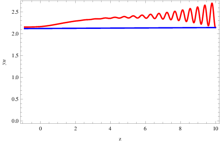
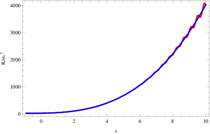
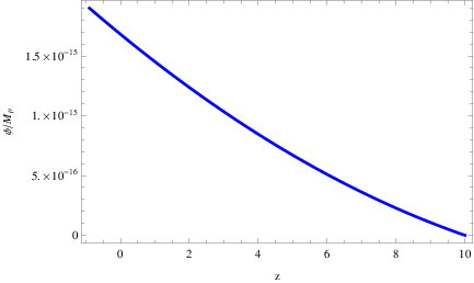
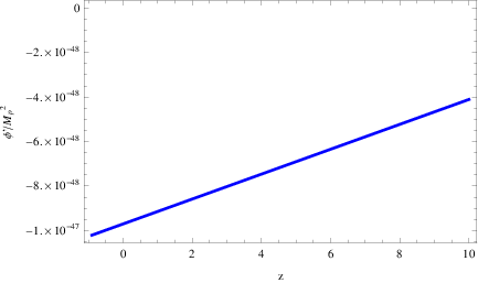
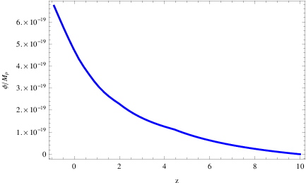
At this point let us present in detail the results of our numerical analysis. We shall focus on the behavior of the most important cosmological quantities, and of the most important statefinder functions that are used in the literature. Let us start with the statefinder function and the curvature , and in Fig. 1 we present the plots of (left plot), and of (right plot) for the -Essence gravity (blue curves) and for the power-law corrected model (red curves) as functions of the redshift. As it is obvious in both the plots, the dark energy oscillations are completely absent from the -Essence gravity theory, at least for redshifts up to . Also, it might seem that for the -Essence gravity theory, is constant, however this is not true, for example at we have while at redshift we have . Also in Fig. 2 we present the plots of (left plot) and of (right plot) for the -Essence gravity model as functions of the redshift. As it can be seen, the values of the scalar field increase as the redshift drops. It is also notable that if we choose an initial condition at , the scalar field takes negative values, but we did not study more this case. Let us proceed to the behavior and values of some important cosmological quantities, starting with the dark energy EoS parameter , which in terms of is given below,
| (42) |
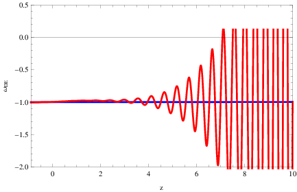
Notably, the dark energy EoS parameter is also a statefinder quantity since it depends implicitly on and its higher first order derivatives. The value of the EoS parameter at present time is evaluated to be for the -Essence gravity model, which is compatible with the latest Planck 2018 data Aghanim:2018eyx values . Furthermore, in Fig. 3 we present the plot of the dark energy EoS parameter for the -Essence gravity (blue curve) and for the power-law corrected model (red curve) as functions of the redshift. In the plot we can see clearly that in the power-law corrected model case (red curve) the oscillations are strongly pronounced as the redshift increases, and in contrast, in the -Essence gravity case, the oscillations are completely absent. Also it is notable that in the -Essence gravity case, the dark energy EoS parameter is slowly varying, with , while as we mentioned, the value at redshift zero is . In Table 1 we gathered all the results for several statefinder and cosmological quantities, for both the -Essence gravity and power-law corrected models, and also the Planck and the CDM model values. Another important cosmological quantity is the dark energy density parameter , which in terms of is given below,
| (43) |
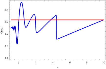
The value of at present time, for the -Essence gravity model is which is compatible with the latest Planck value . Note also that the power-law corrected model yields . Let us now consider the behavior of several well-known statefinder quantities, and we shall be interested in the deceleration parameter , the jerk parameter , the parameter Sahni:2014ooa and finally the parameter Sahni:2002fz, which are given below,
| (44) | ||||
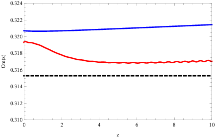
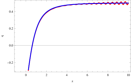
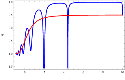
All the statefinder quantities are valuable for the study of the dark energy era, since they depend solely on the Hubble rate and its higher derivatives, hence they depend explicitly on the geometry of spacetime via the Hubble rate. The values of the aforementioned statefinder quantities for the CDM model are presented in Table 1 where we also present the corresponding values for the -Essence gravity model and for the power-law corrected model, for several redshifts. Let us firstly consider the statefinder and in Fig. 4 we present the plots of for the -Essence gravity (blue curve), for the power-law corrected model (red curve) and the CDM model (black dashed curve) as functions of the redshift. As it can be seen, for this specific statefinder quantity, there are differences between the three models, and also no oscillations are observed in the gravity related models, as expected since depends only on the Hubble rate and not on its derivatives. Accordingly in Fig. 5 we present the plot of the deceleration parameter as a function of the redshift, for the -Essence gravity (blue curve), for the power-law corrected model (red curve). In this case, the oscillations in the -Essence gravity model are completely eliminated, while these are present for the power-law corrected model. It is notable that both models are almost indistinguishable from the CDM model.
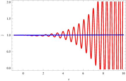
Finally, in Fig. 6 we present the plots of the statefinder function jerk (left plot) and the of (right plot) for the -Essence gravity (blue curves), for the power-law corrected model (red curves). In this case too, the oscillations are completely absent in the -Essence gravity case. Also, we need to note that the jerk for the -Essence gravity case is almost indistinguishable from the CDM value, however it is not constant, as is probably inferred from Fig. 6, it is slowly varying though. For example its value at a redshift is while at is , which are both very close to the CDM value . In Table 1 we gather the values of several cosmological quantities and statefinders for various redshifts values, for the -Essence gravity and the power-law corrected models, and we also quote the corresponding CDM values, the latest Planck constraints or SNe Ia constraints applying for the deceleration parameter. All the models are viable, however the -Essence gravity model seems to be more close to the CDM model for most of the quantities considered.
| Cosmological Parameter | Odintsov-Oikonomou | -Essence | CDM | Planck 2018 or SNe IA22 2 For the deceleration parameter only, based on Ref. Kumar:2011sw |
| Gravity Model Value | Gravity Value | |||
| 0.683948 | 0.679553 | - | ||
| -0.995205 | -0.999667 | - | ||
| 0.319364 | 0.320707 | - | ||
| -0.520954 | -0.51894 | -0.535 | (SNe Ia data) Kumar:2011sw | |
| 1.00319 | 0.99952 | 1 | - | |
| 1.19873 | 1.00362 | 1 | - | |
| 4.25181 | 1.00677 | 1 | - | |
| -0.00104169 | 0.00015711 | 0 | - |
In conclusion, our results indicate that the effect of the -Essence terms on the late-time phenomenology of gravity is very specific, and particularly, it completely eliminates the dark energy oscillations. These dark energy oscillations were present for the power-law corrected model especially at large redshifts, and were more pronounced for quantities that contained higher derivatives of the Hubble rate. As we demonstrated though, the -Essence terms utterly change the picture, by completely eliminating the oscillations and more importantly they also provide a better fit to the CDM model for most of the statefinder quantities we considered, especially the jerk and the deceleration parameter.
Another issue that is worth mentioning is the effect of initial conditions of the scalar field on the whole numerical study. It seems that the same picture occurs for a wide range of initial conditions values, for example similar results are obtained if we choose,
| (45) |
but it notable that a stiff system is obtained if . Another important issue worthy of mentioning is the combined effect that possibly the and the -Essence terms have. Particularly, the is known to eliminate the dark energy singularities Bamba:2008ut; Appleby:2009uf and refines in general the behavior of terms that contain higher derivatives of the Hubble rate, so perhaps the combined effect of the -Essence terms with the term eliminates completely the dark energy oscillations. Let us note that the dark energy singularities are connected with non-linear oscillations of the curvature scalar, during which a finite-time (sudden) singularity occurs in the curvature. For more details on this issue and on the way that the term cures the singularities, we refer the reader to Bamba:2008ut; Appleby:2009uf.
Finally, the parameters that strongly affect the late-time phenomenology are and , with being the coefficient of the higher order kinetic term in the Lagrangian , and is the exponent of in the gravity of Eq. (34). In fact, for a specific range of values of these two parameters, the late-time phenomenology of the -Essence gravity dramatically changes, and interesting physical results are obtained. In the next section we study in brief a phenomenologically interesting situation.
Let us note here that we performed all the above calculations by using the Planck 2018 value for the Hubble rate, namely the one appearing in Eq. (35), that is or equivalently eV, but in principle one could use the value predicted by other sources different from the CMB, like the ones in Refs. Aylor:2018drw; Wong:2019kwg; Verde:2019ivm; Knox:2019rjx; Riess:2016jrr; Migkas:2017vir; Ramos-Ceja:2019zxt, which predict a tension in the value of . If we use the value , the whole analysis we performed in this section shall change as it is conceivable, and in order for a correct viable late-time phenomenology to be obtained, the values of the free parameters must change. For example, if we use the value or equivalently eV, the plots we presented in this section will change. In Fig. 7 we present the comparison of the redshift dependence of for the power-law corrected model, for (red curve) and (black dashed curve), for the same values of the parameters used in the text of this section. As it can be seen, there are some changes, and this will be more apparent if we evaluate the value of , which by choosing we get , which is slightly different from the value found in Table 1 for , namely . The slight difference is caused by the change in the parameter , which for the value is equal to eV2 while when the value is used, the value of becomes eV2. The same applies for the -Essence gravity theory, but we omit the details for brevity.

Before closing, it is worth recalling the choices we assigned to the free parameters of model, which is important in order to understand how much constrained is the model. Essentially, the parameters that are free, without any direct correlation with the observational data, are , , appearing in the gravity model of Eq. (34), and the parameters and related to the coupling and the exponent of the higher order kinetic term in Eq. Eq. (31). The choice of we assumed in the text, was , and this was for simplicity reasons, because the quadratic higher order term is the simplest case we can have. Now the parameter was chosen eV2 for two reasons, firstly in order for it to be of the order of the present day cosmological constant, and secondly in order the fine tuning on this parameter leads to more aesthetically optimal values for the parameters and , and more importantly all the choices lead to a viable cosmology. The parameter must be in the interval , so if we choose eV2, the values and result to a phenomenologically viable late-time phenomenology Odintsov:2020nwm. A slight change in might require not so aesthetically appealing values for and in order to achieve a viable late-time phenomenology, for instance and for eV2. Now the parameter is the only one that requires fine tuning, in order to obtain a viable late-time phenomenology for the -Essence gravity model, and the choice was appearing in Eq. (38).
IV Dynamically Screened Dark Energy Era at Low Redshifts
One of the latest observations in the last decade was the measurement of the Hubble rate at low redshift , with value Delubac:2014aqe. It must be mentioned the result of Delubac:2014aqe, which indicates that the Hubble rate at higher redshift increases, is also supported by other groups in the literature, see for example Moresco:2016mzx; Guo:2015gpa; Stern:2009ep; Chuang:2012qt, however, other measurements at the same redshift do not exist to our knowledge, so caution is needed. For the purposes of this article, we shall assume that the measurement of Delubac:2014aqe is correct, but in principle, in order to consider this result legitimate, this value has to be confirmed.
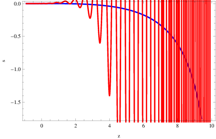
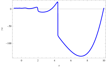
There are two ways to interpret the result of Delubac:2014aqe, if it is assumed to be correct, one to substitute in the Friedmann equation (23), which would imply that which is obviously in conflict with the CMB value reported by the Planck data Aghanim:2018eyx. Obviously, this would be a curious result, in the absence of dark energy, so the second way to interpret it would be to assume that dark energy terms are present, and these would result to negative at Sahni:2014ooa. It is not the first time that negative dark energy density appears in the literature, see for example Refs. Ahmed:2002mj; Cardenas:2014jya and references therein. What we would like to briefly demonstrate in this subsection is the possibility to generate a negative contribution for redshifts , without the need of introducing a compensating dark energy term by hand, as it is done in Ref. Sahni:2014ooa. In fact, the -Essence gravity framework generates such a phenomenological behavior, by simply choosing appropriately the parameters of the model. We shall again consider the -Essence gravity model of the previous section, with the same conventions for the cosmological parameters, and the same initial conditions, with the difference that we choose and also the power of the term to be . Now, a negative contribution in the context of our work, would imply negative values of the statefinder function , and this is the aim of this subsection, to demonstrate that this is possible by using the -Essence gravity theory framework. We numerically solved the Friedmann equation, and the results of the behavior of the statefinder function as a function of the redshift are presented in the left plot of Fig. 8, while in the right plot we present the behavior of . As it can be seen, at the function develops negative values, and as the redshift decreases, increases until present time. In Table 2 we quote the values of the statefinder for various redshifts for both the compensating -Essence gravity and for the power-law corrected model of the previous section. As it can be seen, for redshifts the differences are quite significant.
| -Essence Gravity | power-law corrected model Value | |
|---|---|---|
| 2.18372 | 2.16471 | |
| 2.85154 | 2.18795 | |
| 1.1292 | 2.22296 | |
| 3.19358 | 2.25955 | |
| 0.0617874 | 2.28988 | |
| -4.18054 | 2.29146 | |
| -8.89681 | 2.30763 | |
| 1.49666 | 2.36204 |
Thus the -Essence gravity theoretical framework provides a natural compensating dark energy mechanism, which we do not introduce by hand. We shall call it for the purposes of this paper compensating -Essence gravity.
It is worth investigating further the phenomenology of this case, so we evaluated the dark energy EoS parameter at present time and also the dark energy density parameter , and the results are,
| (46) |
which are both compatible with the latest Planck constraints and . In general, by analyzing the statefinder quantities it turns out that the resulting phenomenology is marginally appealing, though peculiar and quite different from the case studied in the previous section. In order to see this more clearly, we chose to present in Fig. 10 the plots of the deceleration parameter (left plot) and the statefinder (right plot), for the compensating -Essence gravity model (blue curves) and the CDM model (red curves). As it is obvious from the plots, the compensating -Essence gravity model is quite different from the CDM model, and only at very small redshifts near the present-time era there is some overlap between the two models, at least when the deceleration parameter is considered. It is worth quoting here the values of the deceleration parameter and statefinder for for the compensating -Essence gravity, and these are,
| (47) |
which are quite close to the CDM values and . We refrain from going into further details, since the general picture is obvious, the result is that we obtain a marginally compatible to the CDM phenomenology, only at low redshifts, while at larger redshifts, there are differences. However, with the compensating -Essence gravity model we obtain negative dark energy density at nearly , which can explain the observational values of the Hubble rate Delubac:2014aqe at the same redshift. Our model presented in this section offers a phenomenological description which can provide phenomenologically acceptable values to some of the cosmological quantities of interest at redshift zero (present day), like the , , the deceleration parameter and the statefinder , and also can yield negative values for the statefinder at redshift . However, the model cannot be considered a fully correct description of the Universe, neither at present time, nor at higher redshifts, since the overall behavior of some observable quantities is not phenomenologically acceptable.
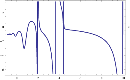
For example, in Fig. 9 we plot for redshifts for the compensating -Essence gravity model, and the result is rather unappealing and phenomenologically not acceptable, although the value of at redshift zero is phenomenologically acceptable. Also the blue curves in Fig. 9 do not provide an optimal fit to the CDM model. What we aimed in this section is to demonstrate that negative values of the statefinder can be obtained by the -Essence gravity model, by appropriately tuning some parameters of the model, and at the same time obtaining compatibility with the observational data for some of the observable quantities at present time. Our description though cannot be considered as a fully viable description of the Universe, and also the results of Ref. Delubac:2014aqe must also be widely accepted in order to further study how our model can be a viable description of the Universe, up to redshifts .
V Conclusions
In this paper we studied the effects of -Essence terms in the late-time phenomenology of gravity in the presence of cold dark matter and radiation perfect fluids. We chose an gravity model which has quite phenomenologically appealing late-time properties, and we assumed that a canonical scalar field term and a higher order kinetic term are also present in the gravitational Lagrangian. With regard to the higher order kinetic term, we studied the case that this term is a quadratic term of the form . The dimensionful parameter plays an important role on the phenomenology as it turns, and in fact, this term in conjunction with an term appearing in the function, crucially affect the late-time phenomenology of the -Essence gravity model. The power-law corrected model apart from the fact that it is similar to the CDM model, it was plagued with the issue of dark energy oscillations at large redshifts. These dark energy oscillations are more pronounced when physical quantities that contain higher derivatives of the Hubble rate are considered. Our aim in this work was to investigate whether these dark energy oscillations are eliminated from the late-time era in the context of -Essence gravity, and as it turns, this occurs for a wide range of initial conditions imposed on the scalar field, and for some values of the parameter which is the coefficient of the quadratic kinetic term . As we demonstrated, a viable late-time phenomenology is produced by the -Essence gravity, without the presence of dark energy oscillations, at least up to a redshift . We studied several cosmological quantities of cosmological interest, such as the dark energy EoS parameter, the dark energy density parameter, and several statefinder quantities. In all the cases, the -Essence gravity model was almost indistinguishable from the CDM model, as for example in the case of the deceleration parameter and the jerk, and in all cases the dark energy oscillations were absent. We also compared directly the power-law corrected model and the -Essence gravity models, to see the difference between the two models and the complete absence of dark energy oscillations for the -Essence gravity model. Apart from this major issue, we also investigated how the -Essence gravity model could explain the 2014 observational data concerning the Hubble rate at redshift . In the presence of dark energy, this observation would require a negative energy density for dark energy. As we demonstrated, by using a specific set of values for the parameter and the exponent of , we achieved a negative energy density for redshifts , and also we demonstrated that the resulting values of the dark energy EoS parameter and of the dark energy density parameter were compatible with the latest Planck data, however the model produced quite different behavior of the statefinder parameters in comparison to the CDM model. Our findings support the idea that the gravity theory and its modifications, viewed as a perfect fluid Capozziello:2018ddp, can mimic a curvature-quintessence like behavior Capozziello:2002rd, at least at late-times. A good question though is how does the -essence term affects the large scale structure formation during the matter domination era. This question is non-trivial to answer in brief though, and a focused simulation on this issue should be performed.
Finally, let us note that in our study we did not take into account the presence of a potential for the scalar field, and we did not investigate at all the case that the scalar field is a phantom scalar. We hope to address these issues in a future work.
Acknowledgments
This work is supported by MINECO (Spain), FIS2016-76363-P, and by project 2017 SGR247 (AGAUR, Catalonia) (S.D.O).
References
- (1) A. G. Riess et al. [Supernova Search Team], Astron. J. 116 (1998) 1009 doi:10.1086/300499 [astro-ph/9805201].
- (2) K. Aylor, M. Joy, L. Knox, M. Millea, S. Raghunathan and W. L. K. Wu, Astrophys. J. 874 (2019) no.1, 4 doi:10.3847/1538-4357/ab0898 [arXiv:1811.00537 [astro-ph.CO]].
- (3) K. C. Wong et al., arXiv:1907.04869 [astro-ph.CO].
- (4) L. Verde, T. Treu and A. G. Riess, Nature Astronomy 2019 doi:10.1038/s41550-019-0902-0 [arXiv:1907.10625 [astro-ph.CO]].
- (5) L. Knox and M. Millea, arXiv:1908.03663 [astro-ph.CO].
- (6) A. G. Riess et al., Astrophys. J. 826 (2016) no.1, 56 doi:10.3847/0004-637X/826/1/56 [arXiv:1604.01424 [astro-ph.CO]].
- (7) K. Migkas and T. H. Reiprich, Astron. Astrophys. 611 (2018) A50 doi:10.1051/0004-6361/201731222 [arXiv:1711.02539 [astro-ph.CO]].
- (8) M. E. Ramos-Ceja, F. Pacaud, T. H. Reiprich, K. Migkas, L. Lovisari and G. Schellenberger, Astron. Astrophys. 626 (2019) A48 doi:10.1051/0004-6361/201935111 [arXiv:1904.10275 [astro-ph.GA]].
- (9) M. Doran and G. Robbers, JCAP 0606 (2006) 026 doi:10.1088/1475-7516/2006/06/026 [astro-ph/0601544].
- (10) A. Bhattacharyya and S. Pal, arXiv:1907.10946 [astro-ph.CO].
- (11) J. Sakstein and M. Trodden, arXiv:1911.11760 [astro-ph.CO].
- (12) S. X. Tian, arXiv:1912.13208 [astro-ph.CO].
- (13) S. Nojiri, S. D. Odintsov and V. K. Oikonomou, arXiv:1912.13128 [gr-qc].
- (14) T. Delubac et al. [BOSS Collaboration], Astron. Astrophys. 574 (2015) A59 doi:10.1051/0004-6361/201423969 [arXiv:1404.1801 [astro-ph.CO]].
- (15) V. Sahni, A. Shafieloo and A. A. Starobinsky, Astrophys. J. 793 (2014) no.2, L40 doi:10.1088/2041-8205/793/2/L40 [arXiv:1406.2209 [astro-ph.CO]].
- (16) S. Nojiri, S. D. Odintsov and V. K. Oikonomou, Phys. Rept. 692 (2017) 1 doi:10.1016/j.physrep.2017.06.001 [arXiv:1705.11098 [gr-qc]].
- (17) S. Nojiri, S. D. Odintsov and D. Saez-Gomez, Phys. Lett. B 681 (2009) 74 doi:10.1016/j.physletb.2009.09.045 [arXiv:0908.1269 [hep-th]].
- (18) S. Capozziello and M. De Laurentis, Phys. Rept. 509 (2011) 167 doi:10.1016/j.physrep.2011.09.003 [arXiv:1108.6266 [gr-qc]].
- (19) V. Faraoni and S. Capozziello, Fundam. Theor. Phys. 170 (2010). doi:10.1007/978-94-007-0165-6
- (20) S. Nojiri and S. D. Odintsov, eConf C 0602061 (2006) 06 [Int. J. Geom. Meth. Mod. Phys. 4 (2007) 115] doi:10.1142/S0219887807001928 [hep-th/0601213].
- (21) S. Nojiri and S. D. Odintsov, Phys. Rept. 505 (2011) 59 doi:10.1016/j.physrep.2011.04.001 [arXiv:1011.0544 [gr-qc]].
- (22) A. de la Cruz-Dombriz and D. Saez-Gomez, Entropy 14 (2012) 1717 doi:10.3390/e14091717 [arXiv:1207.2663 [gr-qc]].
- (23) G. J. Olmo, Int. J. Mod. Phys. D 20 (2011) 413 doi:10.1142/S0218271811018925 [arXiv:1101.3864 [gr-qc]].
- (24) G. Bertone, D. Hooper and J. Silk, Phys. Rept. 405 (2005) 279 doi:10.1016/j.physrep.2004.08.031 [hep-ph/0404175].
- (25) L. Bergstrom, Rept. Prog. Phys. 63 (2000) 793 doi:10.1088/0034-4885/63/5/2r3 [hep-ph/0002126].
- (26) Y. Mambrini, S. Profumo and F. S. Queiroz, Phys. Lett. B 760 (2016) 807 [arXiv:1508.06635 [hep-ph]].
- (27) S. Profumo, arXiv:1301.0952 [hep-ph].
- (28) D. Hooper and S. Profumo, Phys. Rept. 453 (2007) 29 [hep-ph/0701197].
- (29) V. K. Oikonomou, J. D. Vergados and C. C. Moustakidis, Nucl. Phys. B 773 (2007) 19 [hep-ph/0612293].
- (30) S. Nojiri and S. D. Odintsov, Phys. Rev. D 68 (2003) 123512 doi:10.1103/PhysRevD.68.123512 [hep-th/0307288].
- (31) S. Nojiri and S. D. Odintsov, Phys. Lett. B 657 (2007) 238 doi:10.1016/j.physletb.2007.10.027 [arXiv:0707.1941 [hep-th]].
- (32) S. Nojiri and S. D. Odintsov, Phys. Rev. D 77 (2008) 026007 doi:10.1103/PhysRevD.77.026007 [arXiv:0710.1738 [hep-th]].
- (33) G. Cognola, E. Elizalde, S. Nojiri, S. D. Odintsov, L. Sebastiani and S. Zerbini, Phys. Rev. D 77 (2008) 046009 doi:10.1103/PhysRevD.77.046009 [arXiv:0712.4017 [hep-th]].
- (34) S. Nojiri and S. D. Odintsov, Phys. Rev. D 74 (2006) 086005 doi:10.1103/PhysRevD.74.086005 [hep-th/0608008].
- (35) S. A. Appleby and R. A. Battye, Phys. Lett. B 654 (2007) 7 doi:10.1016/j.physletb.2007.08.037 [arXiv:0705.3199 [astro-ph]].
- (36) E. Elizalde, S. Nojiri, S. D. Odintsov, L. Sebastiani and S. Zerbini, Phys. Rev. D 83 (2011) 086006 doi:10.1103/PhysRevD.83.086006 [arXiv:1012.2280 [hep-th]].
- (37) S. D. Odintsov and V. K. Oikonomou, arXiv:2001.06830 [gr-qc].
- (38) K. Bamba, A. Lopez-Revelles, R. Myrzakulov, S. D. Odintsov and L. Sebastiani, Class. Quant. Grav. 30 (2013) 015008 doi:10.1088/0264-9381/30/1/015008 [arXiv:1207.1009 [gr-qc]].
- (39) B. P. Abbott et al. “Multi-messenger Observations of a Binary Neutron Star Merger,” Astrophys. J. 848 (2017) no.2, L12 doi:10.3847/2041-8213/aa91c9 [arXiv:1710.05833 [astro-ph.HE]].
- (40) J. M. Ezquiaga and M. Zumalacarregui, Phys. Rev. Lett. 119 (2017) no.25, 251304 doi:10.1103/PhysRevLett.119.251304 [arXiv:1710.05901 [astro-ph.CO]].
- (41) C. Armendariz-Picon, T. Damour and V. F. Mukhanov, Phys. Lett. B 458 (1999) 209 doi:10.1016/S0370-2693(99)00603-6 [hep-th/9904075].
- (42) T. Chiba, T. Okabe and M. Yamaguchi, Phys. Rev. D 62 (2000) 023511 doi:10.1103/PhysRevD.62.023511 [astro-ph/9912463].
- (43) C. Armendariz-Picon, V. F. Mukhanov and P. J. Steinhardt, Phys. Rev. Lett. 85 (2000) 4438 doi:10.1103/PhysRevLett.85.4438 [astro-ph/0004134].
- (44) J. Matsumoto and S. Nojiri, Phys. Lett. B 687 (2010) 236 doi:10.1016/j.physletb.2010.03.030 [arXiv:1001.0220 [hep-th]].
- (45) C. Armendariz-Picon, V. F. Mukhanov and P. J. Steinhardt, Phys. Rev. D 63 (2001) 103510 doi:10.1103/PhysRevD.63.103510 [astro-ph/0006373].
- (46) T. Chiba, Phys. Rev. D 66 (2002) 063514 doi:10.1103/PhysRevD.66.063514 [astro-ph/0206298].
- (47) M. Malquarti, E. J. Copeland, A. R. Liddle and M. Trodden, Phys. Rev. D 67 (2003) 123503 doi:10.1103/PhysRevD.67.123503 [astro-ph/0302279].
- (48) M. Malquarti, E. J. Copeland and A. R. Liddle, Phys. Rev. D 68 (2003) 023512 doi:10.1103/PhysRevD.68.023512 [astro-ph/0304277].
- (49) L. P. Chimento and A. Feinstein, Mod. Phys. Lett. A 19 (2004) 761 doi:10.1142/S0217732304013507 [astro-ph/0305007].
- (50) L. P. Chimento, Phys. Rev. D 69 (2004) 123517 doi:10.1103/PhysRevD.69.123517 [astro-ph/0311613].
- (51) R. J. Scherrer, Phys. Rev. Lett. 93 (2004) 011301 doi:10.1103/PhysRevLett.93.011301 [astro-ph/0402316].
- (52) J. M. Aguirregabiria, L. P. Chimento and R. Lazkoz, Phys. Rev. D 70 (2004) 023509 doi:10.1103/PhysRevD.70.023509 [astro-ph/0403157].
- (53) C. Armendariz-Picon and E. A. Lim, JCAP 0508 (2005) 007 doi:10.1088/1475-7516/2005/08/007 [astro-ph/0505207].
- (54) L. R. Abramo and N. Pinto-Neto, Phys. Rev. D 73 (2006) 063522 doi:10.1103/PhysRevD.73.063522 [astro-ph/0511562].
- (55) A. D. Rendall, Class. Quant. Grav. 23 (2006) 1557 doi:10.1088/0264-9381/23/5/008 [gr-qc/0511158].
- (56) J. P. Bruneton, Phys. Rev. D 75 (2007) 085013 doi:10.1103/PhysRevD.75.085013 [gr-qc/0607055].
- (57) R. de Putter and E. V. Linder, Astropart. Phys. 28 (2007) 263 doi:10.1016/j.astropartphys.2007.05.011 [arXiv:0705.0400 [astro-ph]].
- (58) E. Babichev, V. Mukhanov and A. Vikman, JHEP 0802 (2008) 101 doi:10.1088/1126-6708/2008/02/101 [arXiv:0708.0561 [hep-th]].
- (59) C. Deffayet, X. Gao, D. A. Steer and G. Zahariade, Phys. Rev. D 84 (2011) 064039 doi:10.1103/PhysRevD.84.064039 [arXiv:1103.3260 [hep-th]].
- (60) N. Kan, K. Shiraishi and M. Yashiki, arXiv:1811.11967 [gr-qc].
- (61) S. Unnikrishnan, V. Sahni and A. Toporensky, JCAP 1208 (2012) 018 doi:10.1088/1475-7516/2012/08/018 [arXiv:1205.0786 [astro-ph.CO]].
- (62) S. Li and A. R. Liddle, JCAP 1210 (2012) 011 doi:10.1088/1475-7516/2012/10/011 [arXiv:1204.6214 [astro-ph.CO]].
- (63) I. D. Gialamas and A. B. Lahanas, arXiv:1911.11513 [gr-qc].
- (64) S. Nojiri, S. D. Odintsov and V. K. Oikonomou, Nucl. Phys. B 941 (2019) 11 doi:10.1016/j.nuclphysb.2019.02.008 [arXiv:1902.03669 [gr-qc]].
- (65) S. D. Odintsov and V. K. Oikonomou, Class. Quant. Grav. 37 (2020) no.2, 025003 doi:10.1088/1361-6382/ab5c9d [arXiv:1912.00475 [gr-qc]].
- (66) N. Aghanim et al. [Planck Collaboration], arXiv:1807.06209 [astro-ph.CO].
- (67) W. Hu and I. Sawicki, Phys. Rev. D 76 (2007) 064004 doi:10.1103/PhysRevD.76.064004 [arXiv:0705.1158 [astro-ph]].
- (68) S. A. Appleby, R. A. Battye and A. A. Starobinsky, JCAP 1006 (2010) 005 doi:10.1088/1475-7516/2010/06/005 [arXiv:0909.1737 [astro-ph.CO]].
- (69) K. Bamba, S. Nojiri and S. D. Odintsov, JCAP 0810 (2008) 045 doi:10.1088/1475-7516/2008/10/045 [arXiv:0807.2575 [hep-th]].
- (70) V. Sahni, T. D. Saini, A. A. Starobinsky and U. Alam, JETP Lett. 77 (2003) 201 [Pisma Zh. Eksp. Teor. Fiz. 77 (2003) 249] doi:10.1134/1.1574831 [astro-ph/0201498].
- (71) S. Kumar, Mon. Not. Roy. Astron. Soc. 422 (2012) 2532 doi:10.1111/j.1365-2966.2012.20810.x [arXiv:1109.6924 [gr-qc]].
- (72) M. Moresco et al., JCAP 1605 (2016) 014 doi:10.1088/1475-7516/2016/05/014 [arXiv:1601.01701 [astro-ph.CO]].
- (73) R. Y. Guo and X. Zhang, Eur. Phys. J. C 76 (2016) no.3, 163 doi:10.1140/epjc/s10052-016-4016-x [arXiv:1512.07703 [astro-ph.CO]].
- (74) D. Stern, R. Jimenez, L. Verde, M. Kamionkowski and S. A. Stanford, JCAP 1002 (2010) 008 doi:10.1088/1475-7516/2010/02/008 [arXiv:0907.3149 [astro-ph.CO]].
- (75) C. H. Chuang and Y. Wang, Mon. Not. Roy. Astron. Soc. 435 (2013) 255 doi:10.1093/mnras/stt1290 [arXiv:1209.0210 [astro-ph.CO]].
- (76) M. Ahmed, S. Dodelson, P. B. Greene and R. Sorkin, Phys. Rev. D 69 (2004) 103523 doi:10.1103/PhysRevD.69.103523 [astro-ph/0209274].
- (77) V. H. Cardenas, Phys. Lett. B 750 (2015) 128 doi:10.1016/j.physletb.2015.08.064 [arXiv:1405.5116 [astro-ph.CO]].
- (78) S. Capozziello, C. A. Mantica and L. G. Molinari, Int. J. Geom. Meth. Mod. Phys. 16 (2018) no.01, 1950008 doi:10.1142/S0219887819500087 [arXiv:1810.03204 [gr-qc]].
- (79) S. Capozziello, Int. J. Mod. Phys. D 11 (2002), 483-492 doi:10.1142/S0218271802002025 [arXiv:gr-qc/0201033 [gr-qc]].