跳到论文正文
W Papers独立论文阅读器 arXiv:2004.08856 论文正文 计算阅读时间 · 0%
引用这篇论文根据当前论文元数据生成,正式投稿前建议核对。


License: arXiv.org perpetual non-exclusive license
arXiv:2004.08856v2 [cs.CR] 22 Dec 2020

Local Differential Privacy based Federated Learning for the Internet of Things

Yang Zhao    Jun Zhao    Mengmeng Yang    Teng Wang    Ning Wang    Lingjuan Lyu    Dusit Niyato       Kwok-Yan Lam    Thanks:  Yang Zhao and Jun Zhao are supported by 1) Nanyang Technological University (NTU) Startup Grant, 2) Alibaba-NTU Singapore Joint Research Institute (JRI), 3) Singapore Ministry of Education Academic Research Fund Tier 1 RG128/18, Tier 1 RG115/19, Tier 1 RT07/19, Tier 1 RT01/19, and Tier 2 MOE2019-T2-1-176, 4) NTU-WASP Joint Project, 5) Singapore National Research Foundation (NRF) under its Strategic Capability Research Centres Funding Initiative: Strategic Centre for Research in Privacy-Preserving Technologies & Systems (SCRIPTS), 6) Energy Research Institute @NTU (ERIAN), 7) Singapore NRF National Satellite of Excellence, Design Science and Technology for Secure Critical Infrastructure NSoE DeST-SCI2019-0012, 8) AI Singapore (AISG) 100 Experiments (100E) programme, and 9) NTU Project for Large Vertical Take-Off & Landing (VTOL) Research Platform. Mengmeng˜Yang and Kwok-Yan˜Lam are supported by the National Research Foundation, Prime Minister’s Office, Singapore under its Strategic Capability Research Centres Funding Initiative. Ning˜Wang is supported by the National Natural Science Foundation of China (61902365) and China Postdoctoral Science Foundation Grant (2019M652473). Dusit˜Niyato is supported by the National Research Foundation (NRF), Singapore, under Singapore Energy Market Authority (EMA), Energy Resilience, NRF2017EWT-EP003-041, Singapore NRF2015-NRF-ISF001-2277, Singapore NRF National Satellite of Excellence, Design Science and Technology for Secure Critical Infrastructure NSoE DeST-SCI2019-0007, A*STAR-NTU-SUTD Joint Research Grant on Artificial Intelligence for the Future of Manufacturing RGANS1906, Wallenberg AI, Autonomous Systems and Software Program and Nanyang Technological University (WASP/NTU) under grant M4082187 (4080), Singapore Ministry of Education (MOE) Tier 1 (RG16/20), and NTU-WeBank JRI (NWJ-2020-004), Alibaba Group through Alibaba Innovative Research (AIR) Program and Alibaba-NTU Singapore Joint Research Institute (JRI). (Corresponding author: Jun Zhao). Yang Zhao, Jun Zhao, Mengmeng˜Yang, Dusit Niyato and Kwok-Yan˜Lam are with School of Computer Science and Engineering, Nanyang Technological University, Singapore, 639798. (Emails: s180049@e.ntu.edu.sg, junzhao@ntu.edu.sg, melody.yang@ntu.edu.sg, dniyato@ntu.edu.sg, kwokyan.lam@ntu.edu.sg). Thanks: Teng˜Wang is with School of Cyberspace Security, Xi’an University of Posts $&$ Telecommunications. (Email: wangteng@xupt.edu.cn). Thanks: Ning˜Wang is with College of Information Science and Engineering, Ocean University of China, 266102. (Email: wangning8687@ouc.edu.cn). Thanks: Lingjuan˜Lyu is with Department of Computer Science, National University of Singapore, 117417. (Email: lingjuanlvsmile@gmail.com).
Abstract

The Internet of Vehicles (IoV) is a promising branch of the Internet of Things. IoV simulates a large variety of crowdsourcing applications such as Waze, Uber, and Amazon Mechanical Turk, etc. Users of these applications report the real-time traffic information to the cloud server which trains a machine learning model based on traffic information reported by users for intelligent traffic management. However, crowdsourcing application owners can easily infer users’ location information, traffic information, motor vehicle information, environmental information, etc., which raises severe sensitive personal information privacy concerns of the users. In addition, as the number of vehicles increases, the frequent communication between vehicles and the cloud server incurs unexpected amount of communication cost. To avoid the privacy threat and reduce the communication cost, in this paper, we propose to integrate federated learning and local differential privacy (LDP) to facilitate the crowdsourcing applications to achieve the machine learning model. Specifically, we propose four LDP mechanisms to perturb gradients generated by vehicles. The proposed Three-Outputs mechanism introduces three different output possibilities to deliver a high accuracy when the privacy budget is small. The output possibilities of Three-Outputs can be encoded with two bits to reduce the communication cost. Besides, to maximize the performance when the privacy budget is large, an optimal piecewise mechanism (PM-OPT) is proposed. We further propose a suboptimal mechanism (PM-SUB) with a simple formula and comparable utility to PM-OPT. Then, we build a novel hybrid mechanism by combining Three-Outputs and PM-SUB. Finally, an LDP-FedSGD algorithm is proposed to coordinate the cloud server and vehicles to train the model collaboratively. Extensive experimental results on real-world datasets validate that our proposed algorithms are capable of protecting privacy while guaranteeing utility.

The development of sensors and communication technologies for Internet of Things (IoT) have enabled a fast and large-scale collection of user data, which has bred new services and applications such as the Waze application that provides the intelligent transportation routing service. This kind of service benefits users’ daily life, but it may raise privacy concerns of sensitive data such as users’ location information. To address these concerns, we propose a hybrid approach that integrates federated learning (FL) [1] with local differential privacy (LDP) [2] techniques. FL can facilitate the collaborative learning with uploaded gradients from users instead of sharing users’ raw data. A honest-but-curious aggregator may be able to leverage users’ uploaded gradients to infer the original data [3, 4]. Thus, we deploy LDP noises to gradients to ensure privacy while not compromising the utility of gradients.

Federated learning with LDP. In addition to LDP mechanisms, FL also provides privacy protection to the data by enabling users to maintain data locally. FedSGD algorithm [5] allows users to submit gradients instead of true data. However, attackers may reverse the gradients to infer original data. By adding LDP noises to the gradients before uploading, we obtain the LDP-FedSGD algorithm, which prevents attackers from deducing original data even though they obtain perturbed gradients. As a result, the FL server gathers and averages users’ submitted perturbed gradients to obtain the averaged result to update the global model’s parameters.

TABLE I: A comparison of the worst-case variances of existing ϵ\epsilon-LDP mechanisms on a single numeric attribute with a domain [−1,1][-1,1]: Duchi of [6] generating a binary output, Laplace of [7] with the addition of Laplace noise, and the Piecewise Mechanism (PM) of [8]. For an LDP mechanism 𝒜\mathcal{A}, its worst-case variance is denoted by V𝒜V_{\mathcal{A}}. We obtain this table based on results of [8].
Range of ϵ\epsilon Comparison of mechanisms
0<ϵ<1.290<\epsilon<1.29 VDuchi<VPM<VLaplaceV_{\texttt{Duchi}}<V_{\texttt{PM}}<V_{\texttt{Laplace}}
1.29<ϵ<2.321.29<\epsilon<2.32 VPM<VDuchi<VLaplaceV_{\texttt{PM}}<V_{\texttt{Duchi}}<V_{\texttt{Laplace}}
ϵ>2.32\epsilon>2.32 VPM<VLaplace<VDuchiV_{\texttt{PM}}<V_{\texttt{Laplace}}<V_{\texttt{Duchi}}
TABLE II: A comparison of the worst-case variances of our and existing ϵ\epsilon-LDP mechanisms on a single numeric attribute with a domain [−1,1][-1,1]. Three-Outputs and PM-SUB are our main LDP mechanisms proposed in this paper. The results in this table show the advantages of our mechanisms over existing mechanisms for a wide range of privacy parameter ϵ\epsilon.
Range of ϵ\epsilon Comparison of mechanisms
0<ϵ<ln⁡2≈0.690<\epsilon<\ln 2\approx 0.69 VDuchi=VThree-Outputs<VPM-SUB<VPMV_{\texttt{Duchi}}=V_{\texttt{Three-Outputs}}<V_{\texttt{PM-SUB}}<V_{\texttt{PM}}
ln⁡2<ϵ<1.19\ln 2<\epsilon<1.19 VThree-Outputs<VDuchi<VPM-SUB<VPMV_{\texttt{Three-Outputs}}<V_{\texttt{Duchi}}<V_{\texttt{PM-SUB}}<V_{\texttt{PM}}
1.19<ϵ<1.291.19<\epsilon<1.29 VThree-Outputs<VPM-SUB<VDuchi<VPMV_{\texttt{Three-Outputs}}<V_{\texttt{PM-SUB}}<V_{\texttt{Duchi}}<V_{\texttt{PM}}
1.29<ϵ<2.561.29<\epsilon<2.56 VThree-Outputs<VPM-SUB<VPM<VDuchiV_{\texttt{Three-Outputs}}<V_{\texttt{PM-SUB}}<V_{\texttt{PM}}<V_{\texttt{Duchi}}
2.56<ϵ<3.272.56<\epsilon<3.27 VPM-SUB<VThree-Outputs<VPM<VDuchiV_{\texttt{PM-SUB}}<V_{\texttt{Three-Outputs}}<V_{\texttt{PM}}<V_{\texttt{Duchi}}
ϵ>3.27\epsilon>3.27 VPM-SUB<VPM<VThree-Outputs<VDuchiV_{\texttt{PM-SUB}}<V_{\texttt{PM}}<V_{\texttt{Three-Outputs}}<V_{\texttt{Duchi}}

Existing LDP mechanisms. Since the proposal of LDP in [7], various LDP mechanisms have been proposed in the literature. Mechanisms for categorical data are presented in [9, 10, 11]. For numerical data, for which new LDP mechanisms are developed in this paper, prior mechanisms of [7, 6, 8] are discussed as follows. For simplicity, we consider data with a single numeric attribute which has a domain [−1,1][-1,1] (after normalization if the original domain is not [−1,1][-1,1]). Extensions to the case of multiple numeric attributes will be discussed later in the paper.

  • •

    Laplace of [7]. LDP can be understood as a variant of DP, where the difference is the definition of “neighboring data(sets)”. In DP, two datasets are neighboring if they differ in just one record; in LDP, any two instances of the user’s data are neighboring. Due to this connection between DP and LDP, the classical Laplace mechanism (referred to Laplace hereinafter) for DP can thus also be used to achieve LDP. Yet, Laplace may not achieve a high utility for some ϵ\epsilon since ① Laplace does not consider the difference between DP and LDP .

  • •

    Duchi of [6]. In view of the above drawback ① of Laplace, Duchi et al. [6] introduce alternative mechanisms for LDP. For a single numeric attribute, one mechanism, hereinafter referred to Duchi of [6], flips a coin with two possibilities to generate an output, where the probability of each possibility depends on the input. A disadvantage of Duchi is as follows: ② Since the output of Duchi has only two possibilities, the utility may not be high for large ϵ\epsilon (intuitively, for large ϵ\epsilon, the privacy protection is weak so the output should be close to the input which means the output should have many possibilities since the input can take any value in [−1,1][-1,1])11 1 Note that any algorithm satisfying DP or LDP has the following property: the set of possible values for the output does not depend on the input (though the output distribution depends on the input). This can be easily seen by contradiction. Suppose an output yy is possible for input xx but not for x′x^{\prime} (xx and x′x^{\prime} satisfy the neighboring relation in DP or LDP). Then ℙ⁡[y∣x]>0{\mathbb{P}}\left[{y\mid x}\right]>0 and ℙ⁡[y∣x′]=0{\mathbb{P}}\left[{y\mid x^{\prime}}\right]=0, resulting in ℙ⁡[y∣x]>eϵ​ℙ​[y∣x′]{\mathbb{P}}\left[{y\mid x}\right]>e^{\epsilon}{\mathbb{P}}\left[{y\mid x^{\prime}}\right] and hence violating the privacy requirement (ℙ[⋅|⋅]\mathbb{P}[\cdot|\cdot] denotes conditional probability)..

  • •

    Piecewise Mechanism (PM) of [8]. Due to the drawback ① of Laplace, and the drawback ② of Duchi above, Wang et al. [8] propose the Piecewise Mechanism (PM) which achieves higher utility than Duchi for large ϵ\epsilon, since the output range of PM is continuous and has infinite possibilities, instead of just 2 possibilities as in Duchi. In PM, the plot of the output’s probability density function with respect to the output value consists of three “pieces”, among which the center piece has a higher probability than the other two. As the input increases, the length of the center piece remains unchanged, but the length of the leftmost (resp., rightmost) piece increases (resp., decreases). Since PM is tailored for LDP, unlike Laplace for LDP, PM has a strictly lower worst-case variance (i.e., the maximum variance with respect to the input given ϵ\epsilon) than Laplace for any ϵ\epsilon.

Proposing new LDP mechanisms. Based on results of [8], Table I on Page I shows that among the three mechanisms Duchi, Laplace, and PM, in terms of the worst-case variance, Duchi is the best for 0<ϵ<1.290<\epsilon<1.29, while PM is the best for ϵ>1.29\epsilon>1.29. Then a natural research question is that can we propose better or even optimal LDP mechanisms? The optimal LDP mechanism for numeric data is still open in the literature, but the optimal LDP mechanism for categorical data has been discussed by Kairouz et al. [12]. In particular, [12] shows that for a categorical attribute (with a limited number of discrete values), the binary and randomized response mechanisms, are universally optimal for very small and large ϵ\epsilon, respectively. Although [12] handles categorical data, its results can provide the following insight even for continuous numeric data: for very small ϵ\epsilon, a mechanism generating a binary output should be optimal; for very large ϵ\epsilon, the optimal mechanism’s output should have infinite possibilities. This is also in consistent with the results of Table I on Page I. Based on the above insight, intuitively, there may exist a range of medium ϵ\epsilon where a mechanism with three, or four, or five, … output possibilities can be optimal. To this end, our first motivation of proposing new LDP mechanisms is to develop a mechanism with three output possibilities such that the mechanism outperform existing mechanisms of Table I for some ϵ\epsilon. The outcome of the above motivation is our mechanism called Three-Outputs. Since the analysis of Three-Outputs is already very complex, we do not consider a mechanism with four, or five, … output possibilities.

In addition, our second motivation of proposing new LDP mechanisms is that despite the elegance of the Piecewise Mechanism (PM) of [8], we can derive the optimal mechanism PM-OPT under the “piecewise framework” of [8], in order to improve PM. Note that PM-OPT is just optimal under the above framework and may not be the optimal LDP mechanism. Since the expressions for PM-OPT are quite complex, we present PM-SUB which compared with PM-OPT is suboptimal, but has simpler expressions and achieves a comparable utility.

Table II on Page II gives a comparison of our and existing LDP mechanisms. For simplicity, we do not include Laplace in the comparison since Laplace is worse than PM for any ϵ\epsilon according to Table I. As shown in Table II, in terms of the worst-case variance for a single numeric attribute with a domain [−1,1][-1,1], Three-Outputs outperforms Duchi for ϵ>ln⁡2≈0.69\epsilon>\ln 2\approx 0.69 (and is the same as Duchi for ϵ≤ln⁡2\epsilon\leq\ln 2), while PM-SUB beats PM for any ϵ\epsilon; moreover, Three-Outputs outperforms both Duchi and PM for ln⁡2<ϵ<3.27\ln 2<\epsilon<3.27, while PM-SUB beats both Duchi and PM for ϵ>1.19\epsilon>1.19.

We also follow the practice of [8], which combines different mechanisms Duchi and PM to obtain a hybrid mechanism HM. HM has a lower worst-case variance than those of Duchi and PM. In this paper, we combine Three-Outputs and PM-SUB to propose HM-TP. The intuition is as follows. Given ϵ\epsilon, the variances of Three-Outputs and PM-SUB (denoted by Tϵ​(x)T_{\epsilon}(x) and Pϵ​(x)P_{\epsilon}(x)) depend on the input xx, and their maximal values (i.e., the worst-case variances) may be taken at different xx. Hence, for a hybrid mechanism which probabilistically uses Three-Outputs with probability qq or PM-SUB with probability 1−q1-q, given ϵ\epsilon, the worst-case variance maxx⁡(q⋅Tϵ​(x)+(1−q)⋅Pϵ​(x))\max_{x}\left(q\cdot T_{\epsilon}(x)+(1-q)\cdot P_{\epsilon}(x)\right) may be strictly smaller than the minimum of maxx⁡Tϵ​(x)\max_{x}T_{\epsilon}(x) and maxx⁡Pϵ​(x)\max_{x}P_{\epsilon}(x). We optimize qq for each ϵ\epsilon to obtain HM-TP. Due to the already complex expression of PM-OPT, we do not consider the combination of PM-OPT and Three-Outputs.

Contributions. Our contributions can be summarized as follows:

  • •

    Using the LDP-FedSGD algorithm for federated learning in IoV as a motivating context, we present novel LDP mechanisms for numeric data with a continuous domain. Among our proposed mechanisms, Three-Outputs and PM-SUB outperform existing mechanisms for a wide range of ϵ\epsilon, as shown in the theoretical results in Table II and confirmed by experiments. In terms of comparing our Three-Outputs and PM-SUB, we have: Three-Outputs, whose output has three possibilities, is better for small ϵ\epsilon, while PM-SUB, whose output can take infinite possibilities of an interval, has higher utility for large ϵ\epsilon. Our PM-SUB is a slightly suboptimal version of our PM-OPT to simplify the expressions. We further combine Three-Outputs and PM-SUB to obtain a hybrid mechanism HM-TP, which achieves even higher utility.

  • •

    We discretize the continuous output ranges of our proposed mechanisms PM-SUB and PM-OPT. Through the discretization post-processing, we enable vehicles to use our proposed mechanisms. In Section VII, we confirm that the discretization post-processing algorithm maintains utility with our experiments, while reducing the communication cost.

  • •

    Experimental evaluation of our proposed mechanisms on real-world datasets and synthetic datasets demonstrates that our proposed mechanisms achieve higher accuracy in estimating the mean frequency of the data and performing empirical risk minimization tasks than existing approaches.

Organization. In the following, Section I introduces the preliminaries. Then, we introduce related works in Section II. Then, we illustrate the system model and the local differential privacy based FedSGD algorithm in Section III. Section IV presents the problem formation. Section V proposes novel solutions for the single numerical data estimation. Section VI illustrates proposed mechanisms used for multidimensional numerical data estimation. Section VII demonstrates our experimental results. Section VIII concludes the paper.

I Preliminaries

In local differential privacy, users complete the perturbation by themselves. To protect users’ privacy, each user runs a random perturbation algorithm ℳ\mathcal{M}, and then he sends perturbed results to the aggregator. The privacy budget ϵ\epsilon controls the privacy-utility trade-off, and a higher privacy budget means a lower privacy protection. As a result of this, we define local differential privacy as follows:

Definition 1.

(Local Differential Privacy.) Let ℳ\mathcal{M} be a randomized function with domain 𝕏\mathbb{X} and range 𝕐\mathbb{Y}; i.e., ℳ\mathcal{M} maps each element in 𝕏\mathbb{X} to a probability distribution with sample space 𝕐\mathbb{Y}. For a non-negative ϵ\epsilon, the randomized mechanism ℳ\mathcal{M} satisfies ϵ\epsilon-local differential privacy if

|ln⁡ℙℳ​[Y∈S|x]ℙℳ​[Y∈S|x′]|≤ϵ,∀x,x′∈𝕏,∀S⊆𝕐.\displaystyle\bigg|\ln\frac{\mathbb{P}_{\mathcal{M}}[Y\in S|x]}{\mathbb{P}_{\mathcal{M}}[Y\in S|x^{\prime}]}\bigg|\leq\epsilon,~\forall x,x^{\prime}\in\mathbb{X},~\forall S\subseteq\mathbb{Y}. (1)

ℙℳ[⋅|⋅]\mathbb{P}_{\mathcal{M}}[\cdot|\cdot] means conditional probability distribution depending on ℳ\mathcal{M}. In local differential privacy, the random perturbation is performed by users instead of a centralized aggregator. Centralized aggregator only receives perturbed results which make sure that the aggregator is unable to distinguish whether the true tuple is xx or x′x^{\prime} with high confidence (controlled by the privacy budget ϵ\epsilon).

Refer to caption
Fig. 1: Different mechanisms’ worst-case noise variance for one-dimensional numeric data versus the privacy budget ϵ\epsilon.

II Related Work

Recently, local differential privacy has attracted much attention [13, 14, 15, 16, 17, 18, 19, 20]. Several mechanisms for numeric data estimation have been proposed [6, 7, 8, 21]. (i) Dwork et al. [7] propose the Laplace mechanism which adds the Laplace noise to real one-dimensional data directly. The Laplace mechanism is originally used in the centralized differential privacy mechanism, and it can be applied to local differential privacy directly. (ii) For a single numeric attribute with a domain [−1,1][-1,1], Duchi et al. [6] propose an LDP framework that provides output from {−C,C}\{-C,C\}, where C>1C>1. (iii) Wang et al. [8] propose the piecewise mechanism (PM) which offers an output that contains infinite possibilities in the range of [−A,A][-A,A], where A>1A>1. In addition, they apply LDP mechanism to preserve the privacy of gradients generated during machine learning tasks. Both approaches by Duchi et al. [6] and Wang et al. [8] can be extended to the case of multidimensional numerical data.

Deficiencies of existing solutions. Fig. 1 illustrates that when ϵ≤2.3\epsilon\leq 2.3, Laplace mechanism’s worst-case noise variance is larger than that of Duchi et al.’s [22] solution; however, the Laplace mechanism outperforms Duchi et al.’s [22] solution if ϵ\epsilon is larger. The worst-case noise variance in PM is smaller than that of Laplace and Duchi et al.’s [22] solution when ϵ\epsilon is large. The HM mechanism outperforms other existing solutions by taking advantage of Duchi et al.’s [22] solution when ϵ\epsilon is small and PM when ϵ\epsilon is large. However, PM and HM’s outputs have infinite possibilities that are hard to encode. We would like to find a mechanism that can improve the utility of existing mechanisms. In addition, we believe there is a mechanism that retains a high utility and is easy to encode its outputs. Based on the above intuition, we propose four novel mechanisms that can be used by vehicles in Section V.

In addition, LDP has been widely used in the research of IoT [23, 24, 25, 26, 27]. For example, Xu et al. [23] integrate deep learning with local differential privacy techniques and apply them to protect users’ privacy in edge computing. They develop an EdgeSanitizer framework that forms a new protection layer against sensitive inference by leveraging a deep learning model to mask the learned features with noise and minimize data. Choi et al. [24] explore the feasibility of applying LDP on ultra-low-power (ULP) systems. They use resampling, thresholding, and a privacy budget control algorithm to overcome the low resolution and fixed point nature of ULPs. He et al. [25] address the location privacy and usage pattern privacy induced by the mobile edge computing’s wireless task offloading feature by proposing a privacy-aware task offloading scheduling algorithm based on constrained Markov decision process. Li et al. [26] propose a scheme for privacy-preserving data aggregation in the mobile edge computing to assist IoT applications with three participants, i.e., a public cloud center (PCC), an edge server (ES), and a terminal device (TD). TDs generate and encrypt data and send them to the ES, and then the ES submits the aggregated data to the PCC. The PCC uses its private key to recover the aggregated plaintext data. Their scheme provides source authentication and integrity and guarantees the data privacy of the TDs. In addition, their scheme can save half of the communication cost. To protect the privacy of massive data generated from IoT platforms, Arachchige et al. [27] design an LDP mechanism named as LATENT for deep learning. A randomization layer between the convolutional module and the fully connected module is added to the LATENT to perturb data before data leave data owners for machine learning services. Pihur et al. [28] propose the Podium Mechanism which is similar to our PM-SUB, but his mechanism is applicable to DP instead of LDP.

Moreover, federated learning or collaborative learning is an emerging distributed machine learning paradigm, and it is widely used to address data privacy problem in machine learning [1, 29]. Recently, federated learning is explored extensively in the Internet of Things recently [30, 31, 32, 33, 34]. Lim et al. [30] survey federated learning applications in mobile edge network comprehensively, including algorithms, applications and potential research problems, etc. Besides, Lu et al. [32] propose CLONE which is a collaborative learning framework on the edges for connected vehicles, and it reduces the training time while guaranteeing the prediction accuracy. Different from CLONE, our proposed approach utilizes local differential privacy noises to protect the privacy of the uploaded data. Furthermore, Fantacci et al. [33] leverage FL to protect the privacy of mobile edge computing, while Saputra et al. [34] apply FL to predict the energy demand for electrical vehicle networks.

Furthermore, there have been many papers on federated learning and differential privacy such as [35, 36, 37, 38, 31, 39, 40, 41, 42, 43]. For example, Truex et al. [36] utilize both secure multiparty computation and centralized differential privacy to prevent inference over both the messages exchanged in the process of training the model. However, they do not analyze the impact of the privacy budget on performance of FL. Hu et al. [37] propose a privacy-preserving FL approach for learning effective personalized models. They use Gaussian mechanism, a centralized DP mechanism, to protect the privacy of the model. Compared with them, our proposed LDP mechanisms provide a stronger privacy protection using the local differential privacy mechanism. Hao et al. [31] propose a differential enhanced federated learning scheme for industrial artificial industry. Triastcyn et al. [39] employ Bayesian differential privacy on federated learning. They make use of the centralized differential privacy mechanism to protect the privacy of gradients, but we leverage a stronger privacy-preserving mechanism (LDP) to protect each vehicle’s privacy.

Additionally, DP can be applied to various FL algorithms such as FedSGD [5] and FedAvg [1]. FedAvg requires users to upload model parameters instead of gradients in FedSGD. The advantage of FedAvg is that it allows users to train the model for multiple rounds locally before submitting gradients. McMahan et al. [35] propose to apply centralized DP to FedAvg and FedSGD algorithm. In our paper, we deploy LDP mechanisms to gradients in FedSGD algorithm. Our future work is to develop LDP mechanisms for state-of-the-art FL algorithms. Zhao et al. [44] propose a SecProbe mechanism to protect privacy and quality of participants’ data by leveraging exponential mechanism and functional mechanism of differential privacy. SecProbe guarantees the high accuracy as well as privacy protection. In addition, it prevents unreliable participants in the collaborative learning.

III System Model and erential Privacy based FedSGD Algorithm

III-A System Model

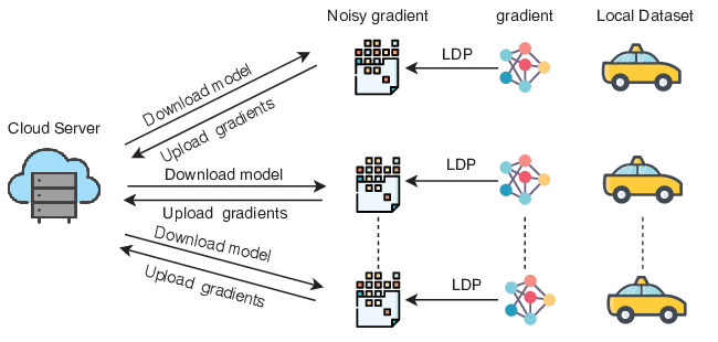
In this work, we consider a scenario where a number of vehicles are connected with a cloud server as Fig. 2. Each vehicle is responsible for continuously performing training and inference locally based on data that it collects and the model initiated by the cloud server. Local training dataset is never uploaded to the cloud server. After finishing predefined epochs locally, the cloud server calculates the average of uploaded gradients from vehicles and updates the global model with the average. The FL aggregator is honest-but-curious or semi-honest, which follows the FL protocol but it will try to learn additional information using received data [36, 45]. With the injected LDP noise, servers or attackers cannot retrieve users’ information by reversing their uploaded gradients [3, 4]. Thus, there is a need to deploy LDP mechanisms to the FL to develop a communication-efficient LDP-based FL algorithm.

Refer to caption
Fig. 2: System Design.

III-B Federated learning with LDP: LDP-FedSGD

In addition, we propose a local differential privacy based federated stochastic gradient descent algorithm (LDP-FedSGD) for our proposed system. Details of LDP-FedSGD are given in Algorithm 1. Unlike the FedAvg algorithm, in the FedSGD algorithm, clients (i.e., vehicles) upload updated gradients instead of model parameters to the central aggregator (i.e., cloud server) [5]. However, compared with the standard FedSGD [5], we add our proposed LDP mechanism proposed in Section VI to prevent the privacy leakage of gradients. Each vehicle locally takes one step of gradient descent on the current model using its local data, and then it perturbs the true gradient with Algorithm 6. The server aggregates and averages the updated gradients from vehicles and then updates the model. To reduce the communication rounds, we separate vehicles into groups, so that the cloud server updates the model after gathering gradient updates from vehicles in a group. In the following sections, we will introduce how we obtain the LDP algorithm in detail.

Server executes:
Server initializes the parameter as θ0\theta_{0};
for tt from 11 to maximal iteration number do 1
Server sends θt−1\theta_{t-1} to vehicles in group GtG_{t};
for each vehicle ii in Group GtG_{t} do 2
   VehicleUpdate(ii, Δ​L\Delta L):Server computes the average of the noisy gradient of group GtG_{t} and updates the parameter from θt−1\theta_{t-1} to θt\theta_{t}: θt←θt−1−η⋅1|Gt|∑i∈Gtℳ(ΔL(θt−1;xi))\theta_{t}\leftarrow\theta_{t-1}-\eta\cdot\frac{1}{|G_{t}|}\sum_{i\in G_{t}}\mathcal{M}(\Delta L(\theta_{t-1};x_{i})), where ηt\eta_{t} is the learning rate;
if θt\theta_{t} and θt−1\theta_{t-1} are close enough or these remains no vehicle which has not participated in the computation then 3
   break;t→t+1;t\rightarrow t+1;VehicleUpdate (ii, Δ​L\Delta L):
Compute the (true) gradient Δ​L​(θt−1,xi)\Delta L(\theta_{t-1};x_{i}), where xix_{i} is vehicle ii’s data;
Use local differential privacy-compliant algorithm ℳ\mathcal{M} to compute the noisy gradient ℳ⁡(Δ⁡(θt−1,xi))\mathcal{M}(\Delta(\theta_{t-1};x_{i}));
Algorithm 1 Local Differential Privacy based FedSGD (LDP-FedSGD) Algorithm.

III-C Comparing LDP-FedSGD with other privacy-preserving federated learning paradigms

The LDP-FedSGD algorithm incorporates LDP into federated learning. In addition to LDP-FedSGD, one may be interested in other ways of using DP in federated learning. To explain them, we categorize combinations of DP and federated learning (or distributed computations in general) by considering the place of perturbation (distributed/centralized perturbation) and privacy granularity (user-level/record-level privacy protection) [46]:

  • •

    Distributed/Centralized perturbation. Note that differential privacy is achieved by introducing perturbation. Distributed perturbation considers an honest-but-curious aggregator, while centralized perturbation needs a trusted aggregator. Both perturbation methods defend against external inference attacks after model publishing.

  • •

    User-level/Record-level privacy protection. In general, a differentially private algorithm ensures that the probability distributions of the outputs on two neighboring datasets do not differ much. The distinction between user-level and record-level privacy protection lies in how neighboring datasets are defined. We define that two datasets are user-neighboring if one dataset can be formed from the other dataset by adding or removing all one user’s records arbitrarily. We define that two datasets are record-neighboring if one dataset can be obtained from the other dataset by changing a single record of one user.

Based on the above, we further obtain four paradigms as follows: 1) ULDP (user-level privacy protection with distributed perturbation), 2) RLDP (record-level privacy protection with distributed perturbation), 3) RLCP (record-level privacy protection with centralized perturbation), and 4) ULCP (user-level privacy protection with centralized perturbation). The details are as follows and can also be found in the second author’s prior work [46].

  1. 1.

    In ULDP, each user ii selects a privacy parameter ϵi\epsilon_{i} and applies a randomization algorithm YiY_{i} such that given any two instances xix_{i} and xi′x_{i}^{\prime} of user ii’s data (which are user-neighboring), and for any possible subset of outputs22 2 For simplicity, we slightly abuse the notation and denote the output of algorithm YiY_{i} (resp., algorithm YY) by YiY_{i} (resp., YY). 𝒴i\mathcal{Y}_{i} of YiY_{i}, we obtain ℙ⁡[Yi∈𝒴i∣xi]≤eϵi×ℙ⁡[Yi∈𝒴i∣xi′]{\mathbb{P}}\left[{Y_{i}\in\mathcal{Y}_{i}\mid x_{i}}\right]\leq e^{\epsilon_{i}}\times{\mathbb{P}}\left[{Y_{i}\in\mathcal{Y}_{i}\mid x_{i}^{\prime}}\right]. Clearly, ULDP is achieved by each user implementing local differential privacy studied in this paper.

  2. 2.

    In RLDP, each user ii selects a privacy parameter ϵi\epsilon_{i} and applies a randomization algorithm YiY_{i} such that for any two record-neighboring instances xix_{i} and xi′x_{i}^{\prime} of user ii’s data (i.e, xix_{i} and xi′x_{i}^{\prime} differ in only one record), and for any possible subset of outputs 𝒴i\mathcal{Y}_{i} of YiY_{i}, we have ℙ⁡[Yi∈𝒴i∣xi]≤eϵi×ℙ⁡[Yi∈𝒴i∣xi′]{\mathbb{P}}\left[{Y_{i}\in\mathcal{Y}_{i}\mid x_{i}}\right]\leq e^{\epsilon_{i}}\times{\mathbb{P}}\left[{Y_{i}\in\mathcal{Y}_{i}\mid x_{i}^{\prime}}\right]. Clearly, in RLDP, what each user does is just to apply standard differential privacy. In contrast, in ULDP above, each user applies local differential privacy.

  3. 3.

    In ϵ\epsilon-RLCP, the aggregator sets a privacy parameter ϵ\epsilon and applies a randomization algorithm YY such that for any user ii, for any two record-neighboring instances xix_{i} and xi′x_{i}^{\prime} of user ii’s data, and for any possible subset of outputs2 𝒴\mathcal{Y} of YY, we obtain ℙ⁡[Y∈𝒴∣xi]≤eϵ×ℙ⁡[Y∈𝒴∣xi′]{\mathbb{P}}\left[{Y\in\mathcal{Y}\mid x_{i}}\right]\leq e^{\epsilon}\times{\mathbb{P}}\left[{Y\in\mathcal{Y}\mid x_{i}^{\prime}}\right]. In other words, in RLCP, the aggregator applies standard differential privacy. For the aggregator to implement RLCP well, typically the aggregator should be able to bound the impact of each record on the information sent from a user to the aggregator. Further discussions on this can be interesting, but we do not present more details since RLCP is not our paper’s focus.

  4. 4.

    In ϵ\epsilon-ULCP, the aggregator sets a privacy parameter ϵ\epsilon and applies a randomization algorithm YY so that for any user ii, for any two instances xix_{i} and xi′x_{i}^{\prime} of user ii’s data (which are user-neighboring), and for any possible subset of outputs 𝒴\mathcal{Y} of YY, we have ℙ⁡[Y∈𝒴∣xi]≤eϵ×ℙ⁡[Y∈𝒴∣xi′]{\mathbb{P}}\left[{Y\in\mathcal{Y}\mid x_{i}}\right]\leq e^{\epsilon}\times{\mathbb{P}}\left[{Y\in\mathcal{Y}\mid x_{i}^{\prime}}\right]. The difference RLCP and ULCP is that RLCP achieves record-level privacy protection while ULCP ensures the stronger user-level privacy protection.

In the case of distributed perturbation, when all users set the same privacy parameter ϵ\epsilon, we refer to ULDP and RLDP above as ϵ\epsilon-ULDP and ϵ\epsilon-RLDP, respectively. Table III presents a comparison of ϵ\epsilon-ULDP, ϵ\epsilon-RLDP, ϵ\epsilon-RLCP, and ϵ\epsilon-ULCP. In this paper’s focus, each user applies ϵ\epsilon-local differential privacy, so our framework is under ULDP. The reasons that we consider ULDP instead of RLDP, RLCP, and ULCP are as follows.

  • •

    We do not consider RLDP which implements perturbation at each user via standard differential privacy, since we aim to achieve user-level privacy protection instead of the weaker record-level privacy protection (a vehicle is a user in our IoV applications and may have multiple records). The motivation is that often much data from a vehicle may be about the vehicle’s regular driver, and it often makes more sense to protect all data about the regular driver instead of just protecting each single record. A similar argument has been recently stated in [35], which incorporates user-level differential privacy into the training process of federated learning for language modeling. Specifically, [35] considers user-level privacy to protect the privacy of all typed words of a user, and explains that such privacy protection is more reasonable than protecting individual words as in the case of record-level privacy. In addition, although we can compute the level of user-level privacy from record-level privacy via the group privacy property of differential privacy (see Theorem 2.2 of [47]), but this may significantly increase the privacy parameter and hence weaken the privacy protection if a user has many records (note that a larger privacy parameter ϵ\epsilon in ϵ\epsilon-DP means weaker privacy protection). More specifically, for a user with mm records, according to the group privacy property [47], the privacy protection strength for the user under ϵ\epsilon-record-level privacy is just as that under m​ϵm\epsilon-user-level privacy (i.e., for a user with mm records, ϵ\epsilon-RLDP ensures m​ϵm\epsilon-ULDP; ϵ\epsilon-RLCP ensures m​ϵm\epsilon-ULCP).

  • •

    We also do not investigate RLCP and ULCP since this paper considers a honest-but-curious aggregator instead of a trusted aggregator. The aggregator is not completely trusted, so the perturbation is implemented at each user (i.e., vehicle in IoV).

TABLE III: We compare different privacy notions in this table. In this paper, we focus on ϵ\epsilon-local differential privacy which achieves user-level privacy protection with distributed perturbation (ULDP). We do not consider record-level privacy protection with distributed perturbation (RLDP) which implements perturbation at each user via standard differential privacy, since we aim to achieve user-level privacy protection instead of the weaker record-level privacy protection (a vehicle is a user in our IoV applications and may have multiple records). We also do not investigate record/user-level privacy protection with centralized perturbation (RLCP/ULCP) since this paper considers a honest-but-curious aggregator instead of a trusted aggregator.
privacy granularity and
place of perturbation
privacy
property
adversary model
ϵ\epsilon-LDP (defined for
distributed perturbation)
ϵ\epsilon-ULDP defend against a honest-but-curious aggregator &external attacks after model publishing
ϵ\epsilon-DP with
distributed perturbation
ϵ\epsilon-RLDP
ϵ\epsilon-DP with
centralized perturbation
ϵ\epsilon-RLCP trusted aggregator; defend against external attacks after model publishing
user-level privacy with
centralized perturbation
ϵ\epsilon-ULCP

IV Problem Formation

Let xx be a user’s true value, and YY be the perturbed value. Under the perturbation mechanism ℳ\mathcal{M}, we use 𝔼ℳ​[Y|x]\mathbb{E}_{\mathcal{M}}[Y|x] to denote the expectation of the randomized output YY given input xx. Varℳ​[Y|x]\textup{Var}_{\mathcal{M}}[Y|x] is the variance of output YY given input xx. MaxVar​(ℳ)\textup{MaxVar}(\mathcal{M}) denotes the worst-case Varℳ​[Y|x]\textup{Var}_{\mathcal{M}}[Y|x]. We are interested in finding a privatization mechanism ℳ\mathcal{M} that minimizes MaxVar​(ℳ)\textup{MaxVar}(\mathcal{M}) by solving the following constraint minimization problem:

minℳ⁡MaxVar​(ℳ),\displaystyle\min_{\mathcal{M}}\textup{MaxVar}(\mathcal{M}),
s.t.​Eq.(1),\displaystyle~\textup{s.t.}~\textup{Eq}.~(\ref{local-differential-privacy-fomular}),
𝔼ℳ​[Y|x]=x,and\displaystyle~~~~~\mathbb{E}_{\mathcal{M}}[Y|x]=x,~\textup{and}
ℙℳ​[Y∈𝕐|x]=1.\displaystyle~~~~~\mathbb{P}_{\mathcal{M}}[Y\in\mathbb{Y}|x]=1.

The second constraint illustrates that our estimator is unbiased, and the third constraint shows the proper distribution where 𝕐\mathbb{Y} is the range of randomized function ℳ\mathcal{M}. In the following sections, if ℳ\mathcal{M} is clear from the context, we omit the subscript ℳ\mathcal{M} for simplicity.

V Mechanisms for Estimation of A Single Numeric Attribute

To solve the problem in Section IV, we propose four local differential privacy mechanisms: Three-Outputs, PM-OPT, PM-SUB, and HM-TP. Fig. 1 compares the worst-case noise variances of existing mechanisms and our proposed mechanisms. Three-Outputs has three discrete output possibilities, which incurs little communication cost because two bits are enough to encode three different outputs. Moreover, it achieves a small worst-case noise variance in the high privacy regime (small privacy budget ϵ\epsilon). However, to maintain a low worst-case noise variance in the low privacy regime (large privacy budget ϵ\epsilon), we propose PM-OPT and PM-SUB. Both of them achieve higher accuracies than Three-Outputs and other existing solutions when the privacy budget ϵ\epsilon is large. Additionally, we discretize their continuous ranges of output for vehicles to encode using a post-processing discretization algorithm. In the following sections, we will explain our proposed four mechanisms and the post-processing discretization algorithm in detail respectively.

V-A Three-Outputs Mechanism

Now, we propose a mechanism with three output possibilities named as Three-Outputs which is illustrated in Algorithm 2. Three-Outputs ensures low communication cost while achieving a smaller worst-case noise variance than existing solutions in the high privacy regime (small privacy budget ϵ\epsilon). Duchi et al.’s [22] solution contains two output possibilities, and it outperforms other approaches when the privacy budget is small. However, Kairouz et al. [12] prove that two outputs are not always optimal as ϵ\epsilon increases. By outputting three values instead of two, Three-Outputs improves the performance as the privacy budget increases, which is shown in Fig. 1. When the privacy budget is small, Three-Outputs is equivalent to Duchi et al.’s [22] solution.

For notional simplicity, given a mechanism ℳ\mathcal{M}, we often write ℙℳ​[Y=y∣X=x]\mathbb{P}_{\mathcal{M}}[Y=y\mid X=x] as Py←x​(ℳ)P_{y\leftarrow x}(\mathcal{M}) below. We also sometimes omit ℳ\mathcal{M} to obtain ℙ⁡[Y=y∣X=x]\mathbb{P}[Y=y\mid X=x] and Py←xP_{y\leftarrow x}.

Input: tuple x∈[−1,1]x\in[-1,1] and privacy parameter ϵ\epsilon.
Output: tuple Y∈{−C,0,C}Y\in\{-C,0,C\}.
Sampling a random variable uu with the probability distribution as follows:
ℙ[u=−1]=P−C←x,\displaystyle{\mathbb{P}}\left[{u=-1}\right]=P_{-C\leftarrow x},
ℙ[u=0]=P0←x,and\displaystyle{\mathbb{P}}\left[{u=0}\right]=P_{0\leftarrow x},~\textup{and}
ℙ[u=1]=PC←x,\displaystyle{\mathbb{P}}\left[{u=1}\right]=P_{C\leftarrow x},
where P−C←xP_{-C\leftarrow x}, P0←xP_{0\leftarrow x} and PC←xP_{C\leftarrow x} are given in Eq. (2), Eq. (3) and Eq. (4).
if u=−1u=-1 then 1
Y=−CY=-C; else if u=0u=0 then 2
Y=0Y=0; else 3
Y=CY=C; return YY;
Algorithm 2 Three-Outputs Mechanism for One-Dimensional Numeric Data.

Given a tuple x∈[−1,1]x\in[-1,1], Three-Outputs returns a perturbed value YY that equals −C-C, 00 or CC with probabilities defined by

P−C←x={1−P0←02+(1−P0←02−eϵ−P0←0eϵ​(eϵ+1))​x,if​0≤x≤1,1−P0←02+(eϵ−P0←0eϵ+1−1−P0←02)​x,if −1≤x≤0,\displaystyle P_{-C\leftarrow x}\hskip-2.0pt=\hskip-2.0pt\begin{cases}&\hskip-12.0pt\frac{1-P_{0\leftarrow 0}}{2}\hskip-2.0pt+\hskip-2.0pt\left(\frac{1-P_{0\leftarrow 0}}{2}\hskip-2.0pt-\hskip-2.0pt\frac{e^{\epsilon}-P_{0\leftarrow 0}}{e^{\epsilon}(e^{\epsilon}+1)}\right)x,\text{if}~0\leq x\leq 1,\\ &\hskip-12.0pt\frac{1-P_{0\leftarrow 0}}{2}\hskip-2.0pt+\hskip-2.0pt\left(\frac{e^{\epsilon}\hskip-2.0pt-\hskip-2.0ptP_{0\leftarrow 0}}{e^{\epsilon}+1}\hskip-2.0pt-\hskip-2.0pt\frac{1-P_{0\leftarrow 0}}{2}\right)x,\text{if }-1\leq x\leq 0,\end{cases} (2)
PC←x={1−P0←02+(eϵ−P0←0eϵ+1−1−P0←02)​x,if ​0≤x≤1,1−P0←02+(1−P0←02−eϵ−P0←0eϵ​(eϵ+1))​x,if−1≤x≤0,\displaystyle P_{C\leftarrow x}\hskip-2.0pt=\hskip-2.0pt\begin{cases}&\hskip-12.0pt\frac{1-P_{0\leftarrow 0}}{2}\hskip-2.0pt+\hskip-2.0pt\left(\frac{e^{\epsilon}-P_{0\leftarrow 0}}{e^{\epsilon}+1}\hskip-2.0pt-\hskip-2.0pt\frac{1-P_{0\leftarrow 0}}{2}\right)x,\text{if }0\leq x\leq 1,\\ &\hskip-12.0pt\frac{1-P_{0\leftarrow 0}}{2}\hskip-2.0pt+\hskip-2.0pt\left(\frac{1-P_{0\leftarrow 0}}{2}\hskip-2.0pt-\hskip-2.0pt\frac{e^{\epsilon}-P_{0\leftarrow 0}}{e^{\epsilon}(e^{\epsilon}+1)}\right)x,\text{if}-1\leq x\leq 0,\end{cases} (3)
and​P0←x=P0←0+(P0←0eϵ−P0←0)​x,if−1≤x≤1,\displaystyle\textup{and}~P_{0\leftarrow x}=P_{0\leftarrow 0}+(\frac{P_{0\leftarrow 0}}{e^{\epsilon}}-P_{0\leftarrow 0})x,~\textup{if}-1\leq x\leq 1, (4)

where P0←0P_{0\leftarrow 0} is defined by

P0←0:=\displaystyle\hskip-10.0ptP_{0\leftarrow 0}:=
{0,if​ϵ<ln⁡2,−16​(−e2​ϵ−4​eϵ−5CLOSEOPEN+2​Δ0​cos⁡(π3+13​arccos⁡(−Δ12​Δ032))),if​ln⁡2≤ϵ≤ϵ′,eϵeϵ+2,if​ϵ>ϵ′,\displaystyle\hskip-10.0pt\begin{cases}&\hskip-10.0pt0,~~\text{if}~\epsilon<\ln 2,\\ &\hskip-10.0pt-\frac{1}{6}(-e^{2\epsilon}-4e^{\epsilon}-5\\ &+2\sqrt{\Delta_{0}}\cos(\frac{\pi}{3}+\frac{1}{3}\arccos(-\frac{\Delta_{1}}{2\Delta_{0}^{\frac{3}{2}}}))),\text{if}~\ln 2\leq\epsilon\leq\epsilon^{\prime},\\ &\hskip-10.0pt\frac{e^{\epsilon}}{e^{\epsilon}+2},~\text{if}~\epsilon>\epsilon^{\prime},\end{cases} (5)

in which

Δ0\displaystyle\Delta_{0} :=e4​ϵ+14​e3​ϵ+50​e2​ϵ−2​eϵ+25,\displaystyle:=e^{4\epsilon}+14e^{3\epsilon}+50e^{2\epsilon}-2e^{\epsilon}+25, (6)
Δ1\displaystyle\Delta_{1} :=−2​e6​ϵ−42​e5​ϵ−270​e4​ϵ−404​e3​ϵ−918​e2​ϵ\displaystyle:=-2e^{6\epsilon}-42e^{5\epsilon}-270e^{4\epsilon}-404e^{3\epsilon}-918e^{2\epsilon}
+30​eϵ−250,\displaystyle+30e^{\epsilon}-250, (7)
and​ϵ′\displaystyle\textup{and}~\epsilon^{\prime} :=ln⁡(3+652)≈ln⁡5.53.\displaystyle:=\ln\left(\frac{3+\sqrt{65}}{2}\right)\approx\ln 5.53. (8)

Next, we will show how we derive the above probabilities. For a mechanism which uses x∈[−1,1]x\in[-1,1] as the input and only three possibilities −C,0,C-C,0,C for the output value, it satisfies

ϵ-LDP:PC←xPC←x′,P0←xP0←x′,P−C←xP−C←x′∈[e−ϵ,eϵ],\displaystyle\textup{$\epsilon$-LDP}:\frac{P_{C\leftarrow x}}{P_{C\leftarrow x^{\prime}}},\frac{P_{0\leftarrow x}}{P_{0\leftarrow x^{\prime}}},\frac{P_{-C\leftarrow x}}{P_{-C\leftarrow x^{\prime}}}\in[e^{-\epsilon},e^{\epsilon}], (9a)
unbiased estimation:
C⋅PC←x+0⋅P0←x+(−C)⋅P−C←x=x,\displaystyle\quad C\cdot P_{C\leftarrow x}+0\cdot P_{0\leftarrow x}+(-C)\cdot P_{-C\leftarrow x}=x, (9b)
proper distribution:
Py←x≥0​and​PC←x+P0←x+P−C←x=1.\displaystyle\quad P_{y\leftarrow x}\geq 0~\textup{and}~P_{C\leftarrow x}+P_{0\leftarrow x}+P_{-C\leftarrow x}=1. (9c)

To calculate values of PC←xP_{C\leftarrow x}, P0←xP_{0\leftarrow x} and P−C←xP_{-C\leftarrow x}, we use Lemma 1 below to convert a mechanism ℳ1\mathcal{M}_{1} satisfying the requirements in (9a) (9b) (9c) to a symmetric mechanism ℳ2\mathcal{M}_{2}. Then, we use Lemma 2 below to transform the symmetric mechanism further to ℳ3\mathcal{M}_{3} whose worst-case noise variance is smaller than ℳ2\mathcal{M}_{2}’s. Next, we use P0←1P_{0\leftarrow 1} to represent other probabilities, and then we prove that we get the minimum variance when P0←0=eϵ​P0←1P_{0\leftarrow 0}=e^{\epsilon}P_{0\leftarrow 1} using Lemma 3. Finally, Lemma 4 and Lemma 5 are used to obtain values for P0←0P_{0\leftarrow 0} and the worst-case noise variance of Three-Outputs, respectively. Thus, we can obtain values of PC←xP_{C\leftarrow x}, P0←xP_{0\leftarrow x} and P−C←xP_{-C\leftarrow x} using P0←0P_{0\leftarrow 0}. In the following, we will illustrate above processes in detail.

By symmetry, for any x∈[−1,1]x\in[-1,1], we enforce

PC←x=P−C←−x,\displaystyle P_{C\leftarrow x}=P_{-C\leftarrow-x}, (10a)
P0←x=P0←−x,\displaystyle P_{0\leftarrow x}=P_{0\leftarrow-x}, (10b)

where Eq. (10b) can be derived from Eq. (10a). The formal justification of Eq. (10a) (10b) is given by Lemma 1 below. Since the input domain [−1,1][-1,1] is symmetric, we can transform any mechanism satisfying requirements in (9a) (9b) (9c) to a symmetric mechanism while guaranteeing the worst-case noise variance will not increase in Lemma 1. Thus, we can derive probabilities when x∈[−1,0]x\in[-1,0] using probabilities when x∈[0,1]x\in[0,1] based on the symmetry.

Lemma 1.

For a mechanism ℳ1\mathcal{M}_{1} satisfying the requirements in (9a) (9b) (9c), the following symmetrization process to obtain a mechanism ℳ2\mathcal{M}_{2} will not increase (i.e., will reduce or not change) the worst-case noise variance, while mechanism ℳ2\mathcal{M}_{2} still satisfies the requirements in (9a) (9b) (9c). Symmetrization: For x∈[−1,1]x\in[-1,1],

PC←x​(ℳ2)=P−C←−x​(ℳ2)=PC←x​(ℳ1)+P−C←−x​(ℳ1)2,\displaystyle P_{C\leftarrow x}(\mathcal{M}_{2})=P_{-C\leftarrow-x}(\mathcal{M}_{2})=\frac{P_{C\leftarrow x}(\mathcal{M}_{1})+P_{-C\leftarrow-x}(\mathcal{M}_{1})}{2}, (11)
P0←x​(ℳ2)=P0←−x​(ℳ2)=P0←x​(ℳ1)+P0←−x​(ℳ1)2.\displaystyle P_{0\leftarrow x}(\mathcal{M}_{2})=P_{0\leftarrow-x}(\mathcal{M}_{2})=\frac{P_{0\leftarrow x}(\mathcal{M}_{1})+P_{0\leftarrow-x}(\mathcal{M}_{1})}{2}. (12)
Proof.

The proof details are given in Appendix -A of the submitted supplementary file. ∎

Based on Lemma 1, we define a symmetric mechanism as follows.

Symmetric Mechanism. A mechanism under (9a) (9b) (9c) is called a symmetric mechanism if it satisfies Eq. (10a) (10b). In the following, we only consider the symmetric mechanism ℳ2\mathcal{M}_{2}.

Now, we design probabilities for the symmetric mechanism ℳ2\mathcal{M}_{2}. As ℳ2\mathcal{M}_{2} satisfies the unbiased estimation which is a linear relationship, we set probabilities as piecewise linear functions of xx as follows:

Case 1: For x∈[0,1]x\in[0,1],

PC←x\displaystyle P_{C\leftarrow x} =PC←0+(PC←1−PC←0)​x,\displaystyle=P_{C\leftarrow 0}+(P_{C\leftarrow 1}-P_{C\leftarrow 0})x, (13)
P−C←x\displaystyle P_{-C\leftarrow x} =P−C←0−(P−C←0−P−C←1)​x,\displaystyle=P_{-C\leftarrow 0}-(P_{-C\leftarrow 0}-P_{-C\leftarrow 1})x, (14)
P0←x\displaystyle P_{0\leftarrow x} =1−P−C←0−PC←0\displaystyle=1-P_{-C\leftarrow 0}-P_{C\leftarrow 0}
+(P−C←0−PC←0+P−C←1−PC←1)​x.\displaystyle+(P_{-C\leftarrow 0}-P_{C\leftarrow 0}+P_{-C\leftarrow 1}-P_{C\leftarrow 1})x. (15)

Case 2: For x∈[−1,0]x\in[-1,0],

PC←x\displaystyle P_{C\leftarrow x} =PC←0+(PC←0−PC←−1)​x,\displaystyle=P_{C\leftarrow 0}+(P_{C\leftarrow 0}-P_{C\leftarrow-1})x, (16)
P−C←x\displaystyle P_{-C\leftarrow x} =P−C←0−(P−C←−1−P−C←0)​x,\displaystyle=P_{-C\leftarrow 0}-(P_{-C\leftarrow-1}-P_{-C\leftarrow 0})x, (17)
P0←x\displaystyle P_{0\leftarrow x} =1−P−C←0−PC←0\displaystyle=1-P_{-C\leftarrow 0}-P_{C\leftarrow 0}
+(P−C←0−PC←0+P−C←1−PC←1)​x.\displaystyle+(P_{-C\leftarrow 0}-P_{C\leftarrow 0}+P_{-C\leftarrow 1}-P_{C\leftarrow 1})x. (18)

Then, we may assign values to our designed probabilities above. We find that if a symmetric mechanism satisfies Eq. (19a) and Eq. (19b), it obtains a smaller worst-case noise variance. From Lemma 2 below, we enforce

PC←1=eϵ​PC←−1,\displaystyle P_{C\leftarrow 1}=e^{\epsilon}P_{C\leftarrow-1}, (19a)
P−C←−1=eϵ​P−C←1.\displaystyle P_{-C\leftarrow-1}=e^{\epsilon}P_{-C\leftarrow 1}. (19b)

Hence, given a symmetric mechanism ℳ2\mathcal{M}_{2} satisfying Inequality (20), we can transform it to a new symmetric mechanism ℳ3\mathcal{M}_{3} which satisfies Eq. (19a) and Eq. (19b) through processes of Eq. (21) (22) (23) until PC←−1=eϵ​P−C←1P_{C\leftarrow-1}=e^{\epsilon}P_{-C\leftarrow 1}. After transformation, the new mechanism ℳ3\mathcal{M}_{3} achieves a smaller worst-case noise variance than mechanism ℳ2\mathcal{M}_{2}. Therefore, we use the new symmetric mechanism ℳ3\mathcal{M}_{3} to replace ℳ2\mathcal{M}_{2} in the future’s discussion. Details of transformation are in the Lemma 2.

Lemma 2.

For a symmetric mechanism ℳ2\mathcal{M}_{2}, if

PC←1​(ℳ2)<eϵ​PC←−1​(ℳ2),\displaystyle P_{C\leftarrow 1}(\mathcal{M}_{2})<e^{\epsilon}P_{C\leftarrow-1}(\mathcal{M}_{2}), (20)

we set a symmetric mechanism ℳ3\mathcal{M}_{3} as follows: For x∈[−1,1]x\in[-1,1],

PC←x​(ℳ3)=P−C←−x​(ℳ3)\displaystyle P_{C\leftarrow x}(\mathcal{M}_{3})=P_{-C\leftarrow-x}(\mathcal{M}_{3})
=PC←x​(ℳ2)−eϵ​PC←−1​(ℳ2)−PC←1​(ℳ2)eϵ−1,\displaystyle=P_{C\leftarrow x}(\mathcal{M}_{2})-\frac{e^{\epsilon}P_{C\leftarrow-1}(\mathcal{M}_{2})-P_{C\leftarrow 1}(\mathcal{M}_{2})}{e^{\epsilon}-1}, (21)
P−C←x​(ℳ3)=PC←−x​(ℳ3)\displaystyle P_{-C\leftarrow x}(\mathcal{M}_{3})=P_{C\leftarrow-x}(\mathcal{M}_{3})
=P−C←x​(ℳ2)−eϵ​P−C←1​(ℳ2)−P−C←−1​(ℳ2)eϵ−1,\displaystyle=P_{-C\leftarrow x}(\mathcal{M}_{2})-\frac{e^{\epsilon}P_{-C\leftarrow 1}(\mathcal{M}_{2})-P_{-C\leftarrow-1}(\mathcal{M}_{2})}{e^{\epsilon}-1}, (22)
P0←x​(ℳ3)=1−PC←x​(ℳ3)−P−C←x​(ℳ3)\displaystyle P_{0\leftarrow x}(\mathcal{M}_{3})=1-P_{C\leftarrow x}(\mathcal{M}_{3})-P_{-C\leftarrow x}(\mathcal{M}_{3})
=P0←x​(ℳ2)+2​(eϵ​PC←−1​(ℳ2)−PC←1​(ℳ2))eϵ−1.\displaystyle=P_{0\leftarrow x}(\mathcal{M}_{2})+\frac{2(e^{\epsilon}P_{C\leftarrow-1}(\mathcal{M}_{2})-P_{C\leftarrow 1}(\mathcal{M}_{2}))}{e^{\epsilon}-1}. (23)

Moreover, the mechanism ℳ3\mathcal{M}_{3} has a worst-case noise variance smaller than that of ℳ2\mathcal{M}_{2}, while ℳ3\mathcal{M}_{3} still satisfies the requirements in (9a) (9b) (9c).

Proof.

The proof details are given in Appendix -B of the submitted supplementary file. ∎

We have proved that the symmetric mechanism ℳ3\mathcal{M}_{3} has a smaller worst-case noise variance than that of mechanism ℳ2\mathcal{M}_{2} in Lemma 2, and then we use mechanism ℳ3\mathcal{M}_{3} to obtain the relation between P0←1P_{0\leftarrow 1} and P0←0P_{0\leftarrow 0} to find the minimum variance. From Lemma 3 below, we enforce

P0←0=eϵ​P0←1.\displaystyle P_{0\leftarrow 0}=e^{\epsilon}P_{0\leftarrow 1}. (24)

Then, we use the following Lemma 3 to obtain the relation between P0←1P_{0\leftarrow 1} and P0←0P_{0\leftarrow 0}, so that we can obtain PC←xP_{C\leftarrow x}, P0←xP_{0\leftarrow x} and P−C←xP_{-C\leftarrow x} using P0←0P_{0\leftarrow 0}.

Lemma 3.

Given P0←0P_{0\leftarrow 0}, the variance of the output given input xx is a strictly decreasing function of P0←1P_{0\leftarrow 1} and hence is minimized when P0←1=P0←0eϵP_{0\leftarrow 1}=\frac{P_{0\leftarrow 0}}{e^{\epsilon}}.

Proof.

The proof details are given in Appendix -C of the submitted supplementary file. ∎

Lemma 3 shows that we get the minimum variance when P0←1=P0←0eϵP_{0\leftarrow 1}=\frac{P_{0\leftarrow 0}}{e^{\epsilon}}. Hence, we replace eϵ​P0←1e^{\epsilon}P_{0\leftarrow 1} with P0←0P_{0\leftarrow 0}. Then, the variance is equivalent to

Var​[Y|X=x]\displaystyle\textup{Var}[Y|X=x]
=(eϵ+1(eϵ−1)​(1−P0←0eϵ))2​(1−P0←0+(P0←0−P0←0eϵ)​|x|)\displaystyle=\left(\frac{e^{\epsilon}+1}{(e^{\epsilon}-1)(1-\frac{P_{0\leftarrow 0}}{e^{\epsilon}})}\right)^{2}\left(1-P_{0\leftarrow 0}+(P_{0\leftarrow 0}-\frac{P_{0\leftarrow 0}}{e^{\epsilon}})|x|\right)
−x2.\displaystyle\quad-x^{2}.~ (25)

Complete details for obtaining Eq. (25) are in Appendix -C of the submitted supplementary file.

Next, we use Lemma 4 to obtain the optimal P0←0P_{0\leftarrow 0} in Three-Outputs to achieve the minimum worst-case variance as follows:

Lemma 4.

The optimal P0←0P_{0\leftarrow 0} to minimize the maxx∈[−1,1]⁡Var​[Y|x]\max_{x\in[-1,1]}\textup{Var}[Y|x] is defined by Eq. (5).

Proof.

The proof details are given in Appendix -E of the submitted supplementary file. ∎

Remark 1.

Fig. 3 displays how P0←0P_{0\leftarrow 0} changes with ϵ\epsilon in Eq. (5). When the privacy budget ϵ\epsilon is small, P0←0=0P_{0\leftarrow 0}=0. Thus, Three-Outputs is equivalent to Duchi et al.’s [22] solution when P0←0=0P_{0\leftarrow 0}=0. However, as the privacy budget ϵ\epsilon increases, P0←0P_{0\leftarrow 0} increases, which means that the probability of outputting true value increases.

Refer to caption
Fig. 3: Optimal P0←0P_{0\leftarrow 0} if the privacy budget ϵ∈[0,8]\epsilon\in[0,8].

By summarizing above, we obtain P−C←xP_{-C\leftarrow x}, PC←xP_{C\leftarrow x} and P0←xP_{0\leftarrow x} from Eq. (2), Eq. (3) and Eq. (4) using P0←0P_{0\leftarrow 0}.

Then, we can calculate the optimal P0←0P_{0\leftarrow 0} to obtain the minimum worst-case noise variance of Three-Outputs as follows:

Lemma 5.

The minimum worst-case noise variance of Three-Outputs is obtained when P0←0P_{0\leftarrow 0} satisfies Eq. (5).

Proof.

The proof details are given in Appendix -F of the submitted supplementary file. ∎

A clarification about Three-Outputs versus Four-Outputs. One may wonder why we consider a perturbation mechanism with three outputs (i.e., our Three-Outputs) instead of a perturbation mechanism with four outputs (referred to as Four-Outputs), since using two bits to encode the output of a perturbation mechanism can represent four outputs. The reason is as follows. The approach to design Four-Outputs is similar to that for Three-Outputs, but the detailed analysis for Four-Outputs will be even more tedious than that for Three-Outputs (which is already quite complex). Given above reasons, we elaborate Three-Outputs but not Four-Outputs in this paper.

V-B PM-OPT Mechanism

Now, we advocate an optimal piecewise mechanism (PM-OPT) as shown in Algorithm 3 to get a small worst-case variance when the privacy budget is large. As shown in Fig. 1, Three-Outputs’s worst-case noise variance is smaller than PM’s when the privacy budget ϵ<3.2\epsilon<3.2. But it loses the advantage when the privacy budget ϵ≥3.2\epsilon\geq 3.2. As the privacy budget increases, Kairouz et al. [12] suggested to send more information using more output possibilities. Besides, we observe that it is possible to improve Wang et al.’s [8] PM to achieve a smaller worst-case noise variance. Thus, inspired by them, we propose an optimal piecewise mechanism named as PM-OPT with a smaller worst-case noise variance than PM.

Input: tuple x∈[−1,1]x\in[-1,1] and privacy parameter ϵ\epsilon.
Output: tuple Y∈[−A,A]Y\in[-A,A].
Value tt is calculated in the Eq. (30);
Sample uu uniformly at random from [0,1][0,1];
if u<eϵt+eϵu<\frac{e^{\epsilon}}{t+e^{\epsilon}} then 1
Sample YY uniformly at random from [L⁡(ϵ,x,t),R⁡(ϵ,x,t)];[L(\epsilon,x,t),R(\epsilon,x,t)];else 2
Sample YY uniformly at random from [−A,L(ϵ,x,t))∪(R(ϵ,x,t),A];[-A,L(\epsilon,x,t))\cup(R(\epsilon,x,t),A];return YY;
Algorithm 3 PM-OPT Mechanism for One-Dimensional Numeric Data under Local Differential Privacy.
Refer to caption
Fig. 4: The probability density function 𝔽⁡[Y=y|x]{\mathbb{F}}\left[{Y=y|x}\right] of the randomized output YY after applying ϵ\epsilon-local differential privacy.

For a true input x∈[−1,1]x\in[-1,1], the probability density function of the randomized output Y∈[−A,A]Y\in[-A,A] after applying local differential privacy is given by

𝔽⁡[Y=y|x]=\displaystyle\hskip-28.0pt{\mathbb{F}}\left[{Y=y|x}\right]\hskip-2.0pt= c,\displaystyle\hskip-5.0ptc, for y∈[L⁡(ϵ,x,t),R⁡(ϵ,x,t)]y\hskip-3.0pt\in\hskip-3.0pt[L(\epsilon,x,t),R(\epsilon,x,t)], (26a)
𝔽⁡[Y=y|x]=\displaystyle\hskip-28.0pt{\mathbb{F}}\left[{Y=y|x}\right]\hskip-2.0pt= d,\displaystyle\hskip-5.0ptd, for y∈[−A,L(ϵ,x,t))∪(R(ϵ,x,t),A]y\hskip-3.0pt\in\hskip-3.0pt[-A,L(\epsilon,x,t))\cup(R(\epsilon,x,t),A], (26b)

where

c\displaystyle c =eϵ​t​(eϵ−1)2​(t+eϵ)2,\displaystyle=\frac{e^{\epsilon}t(e^{\epsilon}-1)}{2(t+e^{\epsilon})^{2}}, (27)
d\displaystyle d =t⁡(eϵ−1)2​(t+eϵ)2,\displaystyle=\frac{t(e^{\epsilon}-1)}{2(t+e^{\epsilon})^{2}}, (28)
A\displaystyle A =(eϵ+t)​(t+1)t⁡(eϵ−1),\displaystyle=\frac{(e^{\epsilon}+t)(t+1)}{t(e^{\epsilon}-1)}, (29)
L⁡(ϵ,x,t)\displaystyle L(\epsilon,x,t) =(eϵ+t)​(x​t−1)t⁡(eϵ−1),\displaystyle=\frac{(e^{\epsilon}+t)(xt-1)}{t(e^{\epsilon}-1)},
R⁡(ϵ,x,t)\displaystyle R(\epsilon,x,t) =(eϵ+t)​(x​t+1)t⁡(eϵ−1),and\displaystyle=\frac{(e^{\epsilon}+t)(xt+1)}{t(e^{\epsilon}-1)},~\textup{and}
12​e2​ϵ+22/3​e2​ϵ−e4​ϵ3+\displaystyle\hskip-2.5pt\frac{1}{2}\sqrt{e^{2\epsilon}\hskip-1.5pt+\hskip-1.5pt2^{2/3}\sqrt[3]{e^{2\epsilon}\hskip-1.5pt-\hskip-1.5pte^{4\epsilon}}}+
12​2​e2​ϵ−22/3​e2​ϵ−e4​ϵ3+4​eϵ−2​e3​ϵe2​ϵ+22/3​e2​ϵ−e4​ϵ3\displaystyle\hskip-1.5pt\frac{1}{2}\sqrt{2e^{2\epsilon}\hskip-1.5pt-\hskip-1.5pt2^{2/3}\sqrt[3]{e^{2\epsilon}\hskip-1.5pt-\hskip-1.5pte^{4\epsilon}}\hskip 1.0pt+\hskip 1.0pt\frac{4e^{\epsilon}\hskip-1.5pt-\hskip-1.5pt2e^{3\epsilon}}{\sqrt{e^{2\epsilon}\hskip-1.5pt+\hskip-1.5pt2^{2/3}\sqrt[3]{e^{2\epsilon}\hskip-1.5pt-\hskip-1.5pte^{4\epsilon}}}}}
−eϵ2,if​ϵ<ln⁡2,\displaystyle\hskip-1.5pt-\hskip-1.5pt\frac{e^{\epsilon}}{2},\hskip 10.0pt\text{if}\hskip 5.0pt\epsilon<\ln\sqrt{2}, (30a)
−12​e2​ϵ+22/3​e2​ϵ−e4​ϵ3+\displaystyle\hskip-2.5pt-\frac{1}{2}\sqrt{e^{2\epsilon}\hskip-1.5pt+\hskip-1.5pt2^{2/3}\sqrt[3]{e^{2\epsilon}\hskip-1.5pt-\hskip-1.5pte^{4\epsilon}}}\hskip-1.5pt+\hskip-1.5pt
12​2​e2​ϵ−22/3​e2​ϵ−e4​ϵ3−4​eϵ−2​e3​ϵe2​ϵ+22/3​e2​ϵ−e4​ϵ3\displaystyle\frac{1}{2}\sqrt{2e^{2\epsilon}\hskip-1.5pt-\hskip-1.5pt2^{2/3}\sqrt[3]{e^{2\epsilon}\hskip-1.5pt-\hskip-1.5pte^{4\epsilon}}\hskip 1.0pt-\hskip 1.0pt\frac{4e^{\epsilon}\hskip-1.5pt-\hskip-1.5pt2e^{3\epsilon}}{\sqrt{e^{2\epsilon}\hskip-1.5pt+\hskip-1.5pt2^{2/3}\sqrt[3]{e^{2\epsilon}\hskip-1.5pt-\hskip-1.5pte^{4\epsilon}}}}}
−eϵ2,if​ϵ>ln⁡2,\displaystyle\hskip-1.5pt-\hskip-1.5pt\frac{e^{\epsilon}}{2},\hskip 10.0pt~\text{if}~\epsilon>\ln\sqrt{2}, (30b)
3+2​3−12,if​ϵ=ln⁡2.\displaystyle\frac{\sqrt{3+2\sqrt{3}}-1}{\sqrt{2}},\hskip 10.0pt~\text{if}~\epsilon=\ln\sqrt{2}. (30c)

The meaning of tt can be seen from t−1t+1=L⁡(ϵ,1,t)R⁡(ϵ,1,t)\frac{t-1}{t+1}=\frac{L(\epsilon,1,t)}{R(\epsilon,1,t)}. When the input is x=1x=1, the length of the higher probability density function 𝔽⁡[Y=y|x]=eϵ​t​(eϵ−1)2​(t+eϵ)2{\mathbb{F}}\left[{Y=y|x}\right]=\frac{e^{\epsilon}t(e^{\epsilon}-1)}{2(t+e^{\epsilon})^{2}} is R⁡(ϵ,1,t)−L⁡(ϵ,1,t)R(\epsilon,1,t)-L(\epsilon,1,t). R⁡(ϵ,1,t)R(\epsilon,1,t) is the right boundary, and L⁡(ϵ,1,t)L(\epsilon,1,t) is the left boundary. If 0<t<∞0<t<\infty, we can derive limt→0t−1t+1=−1\lim_{t\to 0}\frac{t-1}{t+1}=-1, meaning the right boundary is opposite to the left boundary if tt is close to 00. Since limt→∞t−1t+1=1\lim_{t\to\infty}\frac{t-1}{t+1}=1, it means that the right boundary is equal to the left boundary when tt is close to ∞\infty.

Moreover, Fig. 4 illustrates that the probability density function of Eq. (26b) contains three pieces. If y∈[L⁡(ϵ,x,t),R⁡(ϵ,x,t)]y\in[L(\epsilon,x,t),R(\epsilon,x,t)], the probability density function is equal to cc which is higher than other two pieces y∈[−A,L(ϵ,x,t))y\in[-A,L(\epsilon,x,t)) and y∈(R⁡(ϵ,x,t),A]y\in(R(\epsilon,x,t),A]. We calculate the probability of a variable YY falling in the interval [L⁡(ϵ,x,t),R⁡(ϵ,x,t)][L(\epsilon,x,t),R(\epsilon,x,t)] as ℙ[L(ϵ,x,t)≤Y≤R(ϵ,x,t)]=∫L⁡(ϵ,x,t)R⁡(ϵ,x,t)cdY=eϵt+eϵ{\mathbb{P}}\left[{L(\epsilon,x,t)\leq Y\leq R(\epsilon,x,t)}\right]=\int_{L(\epsilon,x,t)}^{R(\epsilon,x,t)}c~dY=\frac{e^{\epsilon}}{t+e^{\epsilon}}.

Furthermore, we use the following lemmas to establish how we get the value tt in Eq. (26b).

Lemma 6.

Algorithm 3 achieves ϵ\epsilon-local differential privacy. Given an input value xx, it returns a noisy value YY with 𝔼⁡[Y|x]=x\mathbb{E}[Y|x]=x and

Var​[Y|x]=t+1eϵ−1​x2+(t+eϵ)​((t+1)3+eϵ−1)3​t2​(eϵ−1)2.\displaystyle\textup{Var}[Y|x]=\frac{t+1}{e^{\epsilon}-1}x^{2}+\frac{(t+e^{\epsilon})\big((t+1)^{3}+e^{\epsilon}-1\big)}{3t^{2}(e^{\epsilon}-1)^{2}}. (31)
Proof.

The proof details are given in Appendix -I of the submitted supplementary file. ∎

Thus, when x=1x=1, we obtain the worst-case noise variance as follows:

maxx∈[−1,1]⁡Var​[Y|x]=t+1eϵ−1+(t+eϵ)​((t+1)3+eϵ−1)3​t2​(eϵ−1)2.\displaystyle\max_{x\in[-1,1]}\textup{Var}[Y|x]=\frac{t+1}{e^{\epsilon}-1}+\frac{(t+e^{\epsilon})\big((t+1)^{3}+e^{\epsilon}-1\big)}{3t^{2}(e^{\epsilon}-1)^{2}}. (32)

Then, we obtain the optimal tt in Lemma 7 to minimize Eq. (32).

Lemma 7.

The optimal t for mint⁡maxx∈[−1,1]​Var​[Y|x]\min_{t}\max_{x\in[-1,1]}\textup{Var}[Y|x] is Eq. (30).

Proof.

By computing the first-order derivative and second-order derivative of mint⁡maxx∈[−1,1]​Var​[Y|x]\min_{t}\max_{x\in[-1,1]}\textup{Var}[Y|x], we get the optimal tt. The proof details are given in Appendix -D of the submitted supplementary file. ∎

V-C PM-SUB Mechanism

We propose a suboptimal piecewise mechanism (PM-SUB) to simplify the sophisticated computation of tt in Eq. (4) of PM-OPT, and details of PM-SUB are shown in Algorithm 4.

Input: tuple x∈[−1,1]x\in[-1,1] and privacy parameter ϵ\epsilon.
Output: tuple Y∈[−A,A]Y\in[-A,A].
Sample uu uniformly at random from [0,1][0,1];
if u<eϵeϵ/3+eϵu<\frac{e^{\epsilon}}{e^{\epsilon/3}+e^{\epsilon}} then 1
Sample YY uniformly at random from [(eϵ+eϵ/3)​(x​eϵ/3−1)eϵ/3​(eϵ−1),(eϵ+eϵ/3)​(x​eϵ/3+1)eϵ/3​(eϵ−1)];[\frac{(e^{\epsilon}+e^{\epsilon/3})(xe^{\epsilon/3}-1)}{e^{\epsilon/3}(e^{\epsilon}-1)},\frac{(e^{\epsilon}+e^{\epsilon/3})(xe^{\epsilon/3}+1)}{e^{\epsilon/3}(e^{\epsilon}-1)}];else 2
Sample YY uniformly at random from [−A,(eϵ+eϵ/3)​(x​eϵ/3−1)eϵ/3​(eϵ−1))∪((eϵ+eϵ/3)​(x​eϵ/3+1)eϵ/3​(eϵ−1),A];[-A,\frac{(e^{\epsilon}+e^{\epsilon/3})(xe^{\epsilon/3}-1)}{e^{\epsilon/3}(e^{\epsilon}-1)})\cup(\frac{(e^{\epsilon}+e^{\epsilon/3})(xe^{\epsilon/3}+1)}{e^{\epsilon/3}(e^{\epsilon}-1)},A];return YY;
Algorithm 4 PM-SUB Mechanism for One-Dimensional Numeric Data under Local Differential Privacy.

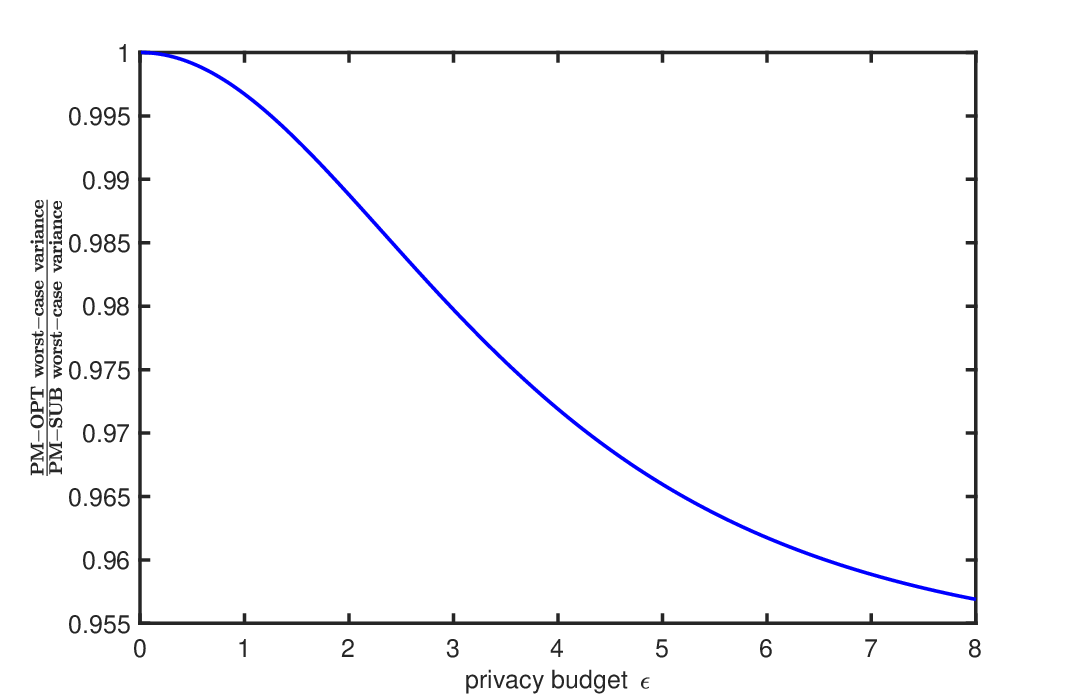
Fig. 1 illustrates that PM-OPT achieves a smaller worst-case noise variance compared with PM, but the parameter tt for PM-OPT in Eq. (30) is complicated to compute. Some vehicles are unable to process the complicated computation. To make tt simple for vehicles to implement, we need to find a simple expression for it while ensuring the mechanism’s performance. Then, we find that Wang et al.’s [8] PM is the case when t=eϵ/2t=e^{\epsilon/2}. Inspired by PM, ln⁡t\ln t and ϵ\epsilon can be linearly related. Then, we find that ln⁡tϵ\frac{\ln t}{\epsilon} is close to 13\frac{1}{3} (tt for PM-OPT in Eq. (30)), so we can set eϵ/3e^{\epsilon/3} as tt in Eq. (26b) for a new mechanism named as PM-SUB. The probability of a variable YY falling in the interval [L⁡(ϵ,x,eϵ/3),R⁡(ϵ,x,eϵ/3)][L(\epsilon,x,e^{\epsilon/3}),R(\epsilon,x,e^{\epsilon/3})] is eϵeϵ/3+eϵ\frac{e^{\epsilon}}{e^{\epsilon/3}+e^{\epsilon}}, and we give the detail of proof in Appendix -J.

Refer to caption
Fig. 5: PM-OPT’s worst-case noise variance versus PM-SUB’s worst-case noise variance.

Similar to PM-OPT, we derive the worst-case noise variance of PM-SUB from Lemma 6 with t=eϵ/3t=e^{\epsilon/3} as follows:

maxx∈[−1,1]⁡Var​[Y|x]=5​e4​ϵ/33​(eϵ−1)2+5​e2​ϵ/33​(eϵ−1)2+2​eϵ(eϵ−1)2.\displaystyle\hskip-5.0pt\max_{x\in[-1,1]}\textup{Var}[Y|x]=\frac{5e^{4\epsilon/3}}{3(e^{\epsilon}-1)^{2}}+\frac{5e^{2\epsilon/3}}{3(e^{\epsilon}-1)^{2}}+\frac{2e^{\epsilon}}{(e^{\epsilon}-1)^{2}}. (33)

As shown in Fig. 5, PM-SUB’s worst-case noise variance is close to PM-OPT’s, but it is smaller than PM’s, which can be observed in Fig. 1.

V-D Discretization Post-Processing

Both PM-OPT and PM-SUB’s output ranges is [−1,1][-1,1] which is continuous, so that there are infinite output possibilities given an input xx. Thus, it is difficult to encode their outputs for vehicles. Hence, we consider to apply a post-processing process to discretize the continuous output range into finite output possibilities. Algorithm 5 shows our discretization post-processing steps.

Input: Perturbed data y∈[−C,C]y\in[-C,C], and domain [−C,C][-C,C] is separated into 2​m2m pieces, where mm is a positive integer.
Output: Discrete data ZZ.
Sample a Bernoulli variable uu such that
ℙ[u=1]=(C⋅(⌊m⋅yC⌋+1)m−y)⋅mC;\displaystyle\hskip-30.0pt{\mathbb{P}}\left[{u=1}\right]=\left(\frac{C\cdot(\left\lfloor\frac{m\cdot y}{C}\right\rfloor+1)}{m}-y\right)\cdot\frac{m}{C};

if u=1u=1 then 1
Z=C⋅⌊m⋅yC⌋mZ=\frac{C\cdot\left\lfloor\frac{m\cdot y}{C}\right\rfloor}{m};else 2
Z=C⋅(⌊m⋅yC⌋+1)mZ=\frac{C\cdot(\left\lfloor\frac{m\cdot y}{C}\right\rfloor+1)}{m};return ZZ;
Algorithm 5 Discretization Post-Processing.

The idea of Algorithm 5 is as follows. We discretize the range of output into 2​m2m parts due to the symmetric range [−C,C][-C,C], and then we obtain 2​m+12m+1 output possibilities. After we get a perturbed data yy, it will fall into one of 2​m2m segments. Then, we categorize it to the left boundary or the right boundary of the segment, which resembles sampling a Bernoulli variable.

Next, we explain how we derive probabilities for the Bernoulli variable. Let the original input be xx. A random variable YY represents the intermediate output after the perturbation and a random variable ZZ represents the output after the discretization. The range of YY is [−C,C][-C,C]. Because the range of output is symmetric with respect to 00, we discretize both [−C,0][-C,0] and [0,C][0,C] into mm parts, where the value of mm depends on the user’ requirement. Thus, we discretize YY to ZZ to take only the following (2​m+1)(2m+1) values:

{i×Cm:integer ​i∈{−m,−m+1,…,m}}.\displaystyle\left\{i\times\frac{C}{m}:\text{integer }i\in\{-m,-m+1,\ldots,m\}\right\}. (34)

When YY is instantiated as y∈[−C,C]y\in[-C,C], we have the following two cases:

  • ①

    If yy is one of the above (2​m+1)(2m+1) values, we set ZZ as yy.

  • ②

    If yy is not one of the above (2​m+1)(2m+1) values, and then there exist some integer k∈{−m,−m+1,…,m−1}k\in\{-m,-m+1,\ldots,m-1\} such that k​Cm<y<(k+1)​Cm\frac{kC}{m}<y<\frac{(k+1)C}{m}. In fact, this gives k<y​mC<k+1k<\frac{ym}{C}<k+1, so we can set k:=⌊y​mC⌋k:=\lfloor\frac{ym}{C}\rfloor. Then conditioning on that YY is instantiated as yy, we set ZZ as k​Cm\frac{kC}{m} with probability k+1−y​mCk+1-\frac{ym}{C} and as (k+1)​Cm\frac{(k+1)C}{m} with probability y​mC−k\frac{ym}{C}-k, so that the expectation of ZZ given Y=yY=y equals yy (as we will show in Eq. (145), this ensures that the expectation of ZZ given the original input as xx equals xx).

The following Lemma 8 shows the probability distribution of assigning yy with a boundary value in the second case above when the intermediate output yy is not one of discrete (2​m+1)(2m+1) values.

Lemma 8.

After we obtain the intermediate output yy after perturbation, we discretize it to a random variable ZZ equal to k​Cm\frac{kC}{m} or (k+1)​Cm\frac{(k+1)C}{m} with the following probabilities:

ℙ⁡[Z=z|Y=y]={k+1−y​mC,if​z=k​Cm,y​mC−k,if​z=(k+1)​Cm.\displaystyle{\mathbb{P}}\left[{Z=z~|~Y=y}\right]=\begin{cases}k+1-\frac{ym}{C},&\text{if}~z=\frac{kC}{m},\\[8.0pt] \frac{ym}{C}-k,&\text{if}~z=\frac{(k+1)C}{m}.\end{cases} (35)
Proof.

The proof details are given in Appendix -K of the submitted supplementary file. ∎

After discretization, the worst-case noise variance does not change or get worse proved by Lemma 9 as follows:

Lemma 9.

Let local differential privacy mechanism be Mechanism ℳ1\mathcal{M}_{1}, and discretization algorithm be Mechanism ℳ2\mathcal{M}_{2}. Let all of output possibilities of Mechanism ℳ1\mathcal{M}_{1} be S1S_{1}, and output possibilities of Mechanism ℳ2\mathcal{M}_{2} be S2S_{2}. S2⊂S1S_{2}\subset S_{1}. When given input xx, ℳ1\mathcal{M}_{1} and ℳ2\mathcal{M}_{2} are unbiased. The worst-case noise variance of Mechanism ℳ2\mathcal{M}_{2} is greater than or equal to the worst-case noise variance of Mechanism ℳ1\mathcal{M}_{1}.

Proof.

The proof details are given in Appendix -L of the submitted supplementary file. ∎

V-E HM-TP Mechanism

Fig. 1 shows that Three-Outputs outperforms PM-SUB when the privacy budget ϵ\epsilon is small, whereas PM-SUB achieves a smaller variance if the privacy budget ϵ\epsilon is large. To fully take advantage of two mechanisms, we combine Three-Outputs and PM-SUB to create a new hybrid mechanism named as HM-TP. Fig. 1 illustrates that HM-TP obtains a lower worst-case noise variance than other solutions.

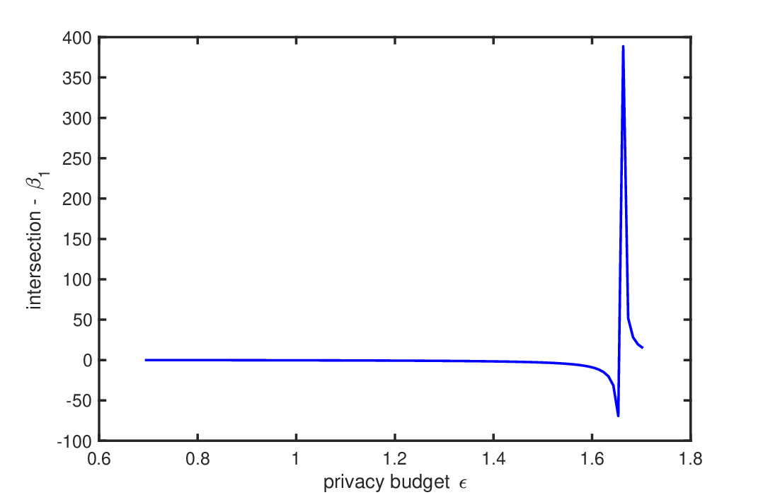
Hence, HM-TP invokes PM-SUB with probability β\beta. Otherwise, it invokes Three-Outputs. We define the noisy variance of HM-TP as Varℋ​[Y|x]\textup{Var}_{\mathcal{H}}[Y|x] given inputs xx as follows:

Varℋ​[Y|x]\displaystyle\textup{Var}_{\mathcal{H}}[Y|x] =β⋅Var𝒫​[Y|x]+(1−β)⋅Var𝒯​[Y|x],\displaystyle=\beta\cdot\textup{Var}_{\mathcal{P}}[Y|x]+(1-\beta)\cdot\textup{Var}_{\mathcal{T}}[Y|x],

where Var𝒫​[Y|x]\textup{Var}_{\mathcal{P}}[Y|x] and Var𝒯​[Y|x]\textup{Var}_{\mathcal{T}}[Y|x] denote noisy outputs’ variances incurred by PM-SUB and Three-Outputs, respectively. The following lemma presents the value of β\beta:

Lemma 10.

The maxx∈[−1,1]⁡Varℋ​[Y|x]\max_{x\in[-1,1]}\textup{Var}_{\mathcal{H}}[Y|x] is minimized when β\beta is Eq. (150). Due to the complicated equation of β\beta, we put it in the appendix.

Proof.

The proof details are given in Appendix -M of the submitted supplementary file. ∎

Since we have obtained the probability β\beta, we can calculate the exact expression for the worst-case noise variance in Lemma 11 as follows:

Lemma 11.

If β\beta satisfies Lemma 10, we obtain the worst-case noise variance of HM-TP as

maxx∈[−1,1]⁡Varℋ​[Y|x]=\displaystyle\max_{x\in[-1,1]}\textup{Var}_{\mathcal{H}}[Y|x]=
{Varℋ​[Y|x∗],if​0<β<2​(eϵ−a)2​(eϵ−1)−a​eϵ​(eϵ+1)22​(eϵ−a)2​(eϵ+t)−a​eϵ​(eϵ+1)2,max⁡{Varℋ​[Y|0],Varℋ​[Y|1]},otherwise,\displaystyle\begin{cases}\textup{Var}_{\mathcal{H}}[Y|x^{*}],\text{if}~0<\beta<\frac{2(e^{\epsilon}-a)^{2}(e^{\epsilon}-1)-ae^{\epsilon}(e^{\epsilon}+1)^{2}}{2(e^{\epsilon}-a)^{2}(e^{\epsilon}+t)-ae^{\epsilon}(e^{\epsilon}+1)^{2}},\\ \max\{\textup{Var}_{\mathcal{H}}[Y|0],\textup{Var}_{\mathcal{H}}[Y|1]\},~~\text{otherwise,}\end{cases}

where x∗:=(β−1)​a​eϵ​(eϵ+1)22​(eϵ−a)2​(β⁡(eϵ+t)−eϵ+1)x^{*}:=\frac{(\beta-1)ae^{\epsilon}(e^{\epsilon}+1)^{2}}{2(e^{\epsilon}-a)^{2}(\beta(e^{\epsilon}+t)-e^{\epsilon}+1)} and a=P0←0a=P_{0\leftarrow 0} which is defined in Eq. (5).

Proof.

The proof details are given in Appendix -U of the submitted supplementary file. ∎

VI Mechanisms for Estimation of Multiple Numeric Attributes

Now, we consider a case in which the user’s data record contains d>1d>1 attributes. There are three existing solutions to collect multiple attributes: (i) The straightforward approach which collects each attribute with privacy budget ϵ/d\epsilon/d. Based on the composition theorem [47], it satisfies ϵ\epsilon-LDP after collecting of all attributes. But the added noise can be excessive if dd is large [8]. (ii) Duchi et al.’s [22] solution, which is rather complicated, handles numeric attributes only. (iii) Wang et al.’s [8] solution is the advanced approach that deals with a data tuple containing both numeric and categorical attributes. Their algorithm requires to calculate an optimal k<dk<d based on the single dimensional attribute’s ϵ\epsilon-LDP mechanism, and a user submits selected kk dimensional attributes instead of dd dimensions.

Input: tuple x∈[−1,1]dx\in[-1,1]^{d} and privacy parameter ϵ\epsilon.
Output: tuple Y∈[−A,A]dY\in[-A,A]^{d}.
Let Y=⟨0,0,…,0⟩Y=\langle 0,0,\dots,0\rangle;
Let k=max⁡{1,min⁡{d,⌊ϵ2.5⌋}}k=\max\{1,\min\{d,\Bigl\lfloor\frac{\epsilon}{2.5}\Bigr\rfloor\}\};
Sample kk values uniformly without replacement from {1,2,…,d}\{1,2,\dots,d\};
for each sampled value jj do 1
Feed x⁡[tj]x[t_{j}] and ϵk\frac{\epsilon}{k} as input to PM-SUB, Three-Outputs or HM-TP, and obtain a noisy value yjy_{j};
Y⁡[tj]=dk​yjY[t_{j}]=\frac{d}{k}y_{j}; return YY;
Algorithm 6 Mechanism for Multiple-Dimensional Numeric Attributes.

Thus, we follow Wang et al.’s [8] idea to extend Section V to the case of multidimensional attributes. Algorithm 6 shows the pseudo-code of our extension for our PM-SUB, Three-Outputs, and HM-TP. Given a tuple x∈[−1,1]dx\in[-1,1]^{d}, the algorithm returns a perturbed tuple YY that has non-zero value on kk attributes, where

k=max⁡{1,min⁡{d,⌊ϵ2.5⌋}},\displaystyle k=\max\{1,\min\{d,\Bigl\lfloor\frac{\epsilon}{2.5}\Bigr\rfloor\}\}, (36)

and Appendix -S of the submitted supplementary file proves our selected kk is optimal after extending PM-SUB, Three-Outputs, and HM-TP to support dd dimensional attributes.

Overall, our algorithm for collecting multiple attributes outperforms existing solutions, which is confirmed by our experiments in the Section VII. But Three-Outputs uses only one more bit compared with Duchi et al.’s [22] solution to encode outputs. Moreover, our Three-Outputs obtains a higher accuracy in the high privacy regime (where the privacy budget is small) and saves many bits for encoding since PM and HM’s continuous output range requires infinite bits to encode, whereas PM-SUB and HM-TP’s advantages are obvious at a large privacy budget. Furthermore, because vehicles can not encode continuous range, we discretize the continuous range of outputs to discrete outputs. Our experiments in Section  confirm that we can achieve similar results to algorithms before discretizing by carefully designing the number of discrete parts. Hence, our proposed algorithms are obviously more suitable for vehicles than existing solutions.

Intuitively, Algorithm 6 requires every user to submit kk attributes instead of dd attributes, such that the privacy budget for each attribute increases from ϵ/d\epsilon/d to ϵ/k\epsilon/k, which helps to minimize the noisy variance. In addition, by setting kk as Eq. (36), algorithm 6 achieves an asymptotically optimal performance while preserving privacy, which we will prove using Lemma 12 and 13. Lemma 12 and 13 are proved in the same way as that of Lemma 44 and 55 in [8].

Lemma 12.

Algorithm 6 satisfies ϵ\epsilon-local differential privacy. In addition, given an input tuple xx, it outputs a noisy tuple YY, such that for any j∈[1,d]j\in[1,d], and each tjt_{j} of those kk attributes is selected uniformly at random (without replacement) from all dd attributes of xx, and then 𝔼⁡[Y⁡[tj]]=x⁡[tj]\mathbb{E}[Y[t_{j}]]=x[t_{j}].

Proof.

Algorithm 6 composes kk numbers of ϵ\epsilon-LDP perturbation algorithms; thus, based on composition theorem of differential mechanism [48], Algorithm 6 satisfies ϵ\epsilon-LDP. As we can see from Algorithm 6, each perturbed output YY equals to dk​yj\frac{d}{k}y_{j} with probability kd\frac{k}{d} or equals to 0 with probability 1−kd1-\frac{k}{d}. Thus, 𝔼⁡[Y⁡[tj]]=kd⋅𝔼⁡[dk⋅yj]=𝔼⁡[yj]=x⁡[tj]\mathbb{E}[Y[t_{j}]]=\frac{k}{d}\cdot\mathbb{E}[\frac{d}{k}\cdot y_{j}]=\mathbb{E}[y_{j}]=x[t_{j}] holds. ∎

Lemma 13.

For any j∈[1,d]j\in[1,d], let Z⁡[tj]=1n​∑i=1nY⁡[tj]Z[t_{j}]=\frac{1}{n}\sum_{i=1}^{n}Y[t_{j}] and X⁡[tj]=1n​∑i=1nx⁡[tj]X[t_{j}]=\frac{1}{n}\sum_{i=1}^{n}x[t_{j}]. With at least 1−β1-\beta probability,

maxj∈[1,d]⁡|Z⁡[tj]−X⁡[tj]|=O⁡(OPENd​ln⁡(d/β))ϵ​n).\max_{j\in[1,d]}|Z[t_{j}]-X[t_{j}]|=O\bigg(\frac{\sqrt{d\ln(d/\beta))}}{\epsilon\sqrt{n}}\bigg).
Proof.

The proof details are given in Appendix -R of the submitted supplementary file. ∎

[Uncaptioned image]
Refer to caption
(a) MX-Numeric
Refer to caption
(b) BR-Numeric
Refer to caption
(c) WISDM-Numeric
Refer to caption
(d) Vehicle-Numeric
Fig. 6: Result accuracy for mean estimation (on numeric attributes).
Refer to caption
(a) μ=0\mu=0
Refer to caption
(b) μ=1/3\mu=1/3
Refer to caption
(c) μ=2/3\mu=2/3
Refer to caption
(d) μ=1\mu=1
Fig. 7: Result accuracy on synthetic datasets with 16 dimensions, each of which follows a Gaussian distribution N⁡(μ,1/16)N(\mu,1/16) truncated to [−1,1][-1,1].
Refer to caption
Refer to caption
(a) MX
Refer to caption
(b) BR
Refer to caption
(c) WISDN
Fig. 8: Logistic Regression.
Refer to caption
Refer to caption
(a) MX
Refer to caption
(b) BR
Refer to caption
(c) WISDN
Fig. 9: Linear Regression.
Refer to caption
(a) MX
Refer to caption
(b) BR
Refer to caption
(c) WISDN
Refer to caption
(d) Vehicle
Fig. 10: Support Vector Machines.
Refer to caption
Refer to caption
(a) MX
Refer to caption
(b) BR
Refer to caption
(c) WISDN
Fig. 11: Result accuracy for mean estimation with discretization post processing on PM, HM, and HM-TP.
Refer to caption
Refer to caption
(a) MX
Refer to caption
(b) BR
Refer to caption
(c) WISDN
Fig. 12: Linear Regression with discretization post processing on PM, HM, and HM-TP (privacy parameter ϵ=4\epsilon=4).
Refer to caption
Refer to caption
(a) MX
Refer to caption
(b) BR
Refer to caption
(c) WISDN
Fig. 13: Logistic Regression with discretization post processing on PM, HM, and HM-TP (privacy budget ϵ=4\epsilon=4).
Refer to caption
(a) MX
Refer to caption
(b) BR
Refer to caption
(c) WISDN
Fig. 14: Linear Regression with discretization post processing on PM, HM, and HM-TP (privacy budget ϵ=4\epsilon=4).
Refer to caption
(a) BR
Fig. 15: Support Vector Machine with discretization post processing on PM, HM, and HM-TP (privacy budget ϵ=5\epsilon=5).

VII Experiments

We implemented both existing solutions and our proposed solutions, including PM-SUB, Three-Outputs, HM-TP proposed by us, PM and HM proposed by Wang et al. [8], Duchi et al.’s [22] solution and the traditional Laplace mechanism. Our datasets include (i) the WISDM Human Activity Recognition dataset [49] is a set of accelerometer data collecting on Android phones from 3535 subjects performing 66 activities, where the domain of the timestamps of the phone’s uptime is removed from the dataset, and the remaining 33 numeric attributes are accelerations in x,y,x,y, and zz directions measured by the Android phone’s accelerometer and 22 categorical attributes; (ii) two public datasets extracted from Integrated Public Use Microdata Series [50] contain census records from Brazil (BR) and Mexico (MX). BR includes 44M tuples and 1616 attributes, of which 66 are numerical and 1010 are categorical. MX contains 4​M4M records and 1919 attributes, of which 55 are numerical and 1414 are categorical; (iii) a Vehicle dataset obtained by collecting from a distributed sensor network, including acoustic (microphone), seismic (geophone), and infrared (polarized IR sensor) [51]. The dataset contains 9852898528 tuples and 101101 attributes, where 100100 attributes are numerical representing information such as the raw time series data observed at each sensor and acoustic feature vectors extracted from each sensor’s microphone. One attribute is categorical denoting different types of vehicles, which are labeled manually by a human operator to ensure high accuracy. Besides, information about vehicles is gathered to find out the type or brand of the vehicle. The Vehicle dataset is also used as the federated learning benchmark by [52]. We normalize the domain of each numeric attribute to [−1,1][-1,1]. In our experiments, we report average results over 100100 runs.

VII-A Results on the Mean Values of Numeric Attributes

We estimate the mean of every numeric attribute by collecting a noisy multidimensional tuple from each user. To compare with Wang et al.’s [8] mechanisms, we follow their experiments and then divide the total privacy budget ϵ\epsilon into two parts. Assume a tuple contains dd attributes which include dnd_{n} numeric attributes and dcd_{c} categorical attributes. Then, we allocate dn​ϵ/dd_{n}\epsilon/d budget to numeric attributes, and dc​ϵ/dd_{c}\epsilon/d to categorical ones, respectively. Our approach of using LDP for categorical data is same as that of Wang et al. [8]. We estimate the mean value for each of the numeric attributes using existing methods: (i) Duchi et al.’s [22] solution handles multiple numeric attributes directly; (ii) when using the Laplace mechanism, it applies ϵ/d\epsilon/d budget to each numeric attribute individually; (iii) PM and HM are from Wang et al. [8]. In Section VI, we evaluate the mean square error (MSE) of the estimated mean values for numeric attributes using our proposed approaches. Fig. 6 presents MSE results as a function of the total budget of ϵ\epsilon in the datasets (WISDM, MX, BR and Vehicle). To simplify the complexity, we use last 66 numerical attributes of the Vehicle dataset to calculate MSE. Overall, our experimental evaluation shows that our proposed approaches outperform existing solutions. HM-TP outperforms existing solutions in all settings, whereas PM-SUB’s MSE is smaller than PM’s when privacy budget ϵ\epsilon is large such as 44, and Three-Outputs’ performance is better at a small privacy budget. Hence, experimental results are in accordance with our theories.

We also run a set of experiments on synthetic datasets that contain numeric attributes only. We create four synthetic datasets, including 1616 numeric attributes where each attribute value is obtained by sampling from a Gaussian distribution with mean value u∈{0,13,23,1}u\in\{0,\frac{1}{3},\frac{2}{3},1\} and standard deviation of 14\frac{1}{4}. By evaluating the MSE in estimating mean values of numeric attributes with our proposed mechanisms, we present our experimental results in Fig. 7. Hereby, we confirm that PM-SUB, Three-Outputs and HM-TP outperform existing solutions.

VII-B Results on Empirical Risk Minimization

In the following experiments, we evaluate the proposed algorithms’ performance using linear regression, logistic regression, and SVM classification tasks. We change each categorical attribute tjt_{j} with kk values into k−1k-1 binary attributes with a domain {−1,1}\{-1,1\}, for example, given tjt_{j}, (i) 11 represents the ll-th (l<kl<k) value on the ll-th binary attribute and −1-1 on each of the rest of k−2k-2 attributes; (ii) −1-1 represents the kk-th value on all binary attributes. After the transformation, the dimension of WISDN is 4343, BR (resp. MX) is 9090 (resp. 9494) and Vehicle is 101101. Since both the BR and MX datasets contain the “total income” attribute, we use it as the dependent variable and consider other attributes as independent variables. The Vehicle dataset is used for SVM [51, 52]. Each tuple in the Vehicle dataset contains 100-dimensional feature and a binary label.

Consider each tuple of data as the dataset of a vehicle, so vehicles calculate gradients and run different LDP mechanisms to generate noisy gradients. Each mini-batch is a group of vehicles. Thus, the centralized aggregator i.e. cloud server updates the model after each group of vehicles send noisy gradients. The experiment involves 88 competitors: PM-SUB, Three-Outputs, HM-TP, PM, HM, Duchi et al.’s solution, Laplace and a non-private setting. We set the regularization factor λ=10−4\lambda=10^{-4} in all approaches. We use 1010-fold cross-validation 55 times to evaluate the performance of each method in each dataset. Fig. 8 and Fig. 10 show that the proposed mechanisms (PM-SUB, Three-Outputs, and HM-TP) have lower misclassification rates than other mechanisms. Fig. 9 shows the MSE of the linear regression model. We ignore Laplace’s result because its MSE clearly exceeds those of other mechanisms. In the selected privacy budgets, our proposed mechanisms (PM-SUB, Three-Outputs, and HM-TP) outperform existing approaches, including Laplace mechanism, Duchi et al.’s solution, PM, and HM.

VII-C Results after Discretization

In this section, we add a discretization post processing step in Algorithm 5 to the implementation of mechanisms with continuous range of outputs, including PM, PM-SUB, HM and HM-TP. To confirm that the discretization is effective, we perform the following experiments. We separate the output domain [−C,C][-C,C] into 20002000 segments, and then we have 20012001 possible outputs given an initial input xx. We add a discretization step to the experiments in Section VII-A. Fig. 11 displays our experimental results. We confirm that our proposed approaches outperform existing solutions in estimating the mean value using three real-world datasets: WISDM, MX, and BR after discretizing.

In addition, we use log regression and linear regression to evaluate the performance after discretization. We repeat the experiments in Section VII-B with an additional discretization post processing step. Fig. 12 and Fig. 13 present our experimental results. Compared with other approaches, the performance is similar to that before discretizing. Furthermore, Fig. 14 illustrates how the accuracy changes as output possibilities increase. It shows that the misclassification rate of the logistic regression task and the MSE of the linear regression task are related to the size of output possibilities. Although incurring with randomness, we find that the misclassification rate and MSE decrease as the number of output possibilities increases. When there are three output possibilities, it incurs randomness. Moreover, Fig. 15 shows that PM-SUB outperforms Three-Outputs, when the number of output possibilities is large. However, when we discretize the range of outputs into 20002000 segments, the performance is satisfactory and similar to the performance with a continuous range of outputs. Hence, our proposed approaches combined with the discretization step help retain the performance while enabling the usage in vehicles.

VIII Conclusion

In this paper, we propose PM-OPT, PM-SUB, Three-Outputs, and HM-TP local differential privacy mechanisms. These mechanisms effectively preserve the privacy when collecting data records and computing accurate statistics in various data analysis tasks, including estimating the mean frequency and machine learning tasks such as SVM classification, logistic regression, and linear regression. Moreover, we integrate our proposed local differential privacy mechanisms with FedSGD algorithm to create an LDP-FedSGD algorithm. The LDP-FedSGD algorithm enables the vehicular crowdsourcing applications to train a machine learning model to predict the traffic status while avoiding the privacy threat and reducing the communication cost. More specifically, by leveraging LDP mechanisms, adversaries are unable to deduce the exact location information of vehicles from uploaded gradients. Then, FL enables vehicles to train their local machine learning models using collected data and then send noisy gradients instead of data to the cloud server to obtain a global model. Extensive experiments demonstrate that our proposed approaches are effective and able to perform better than existing solutions. Further, we intend to apply our proposed LDP mechanisms to deep neural network to deal with more complex data analysis tasks.

References

  • [1] B. McMahan, E. Moore, D. Ramage, S. Hampson, and B. A. y Arcas, “Communication-efficient learning of deep networks from decentralized data,” in Artificial Intelligence and Statistics, 2017, pp. 1273–1282.
  • [2] V. Bindschaedler, R. Shokri, and C. A. Gunter, “Plausible deniability for privacy-preserving data synthesis,” Proceedings of the VLDB Endowment, vol. 10, no. 5, pp. 481–492, 2017.
  • [3] B. Hitaj, G. Ateniese, and F. Perez-Cruz, “Deep models under the GAN: information leakage from collaborative deep learning,” in Proceedings of the 2017 ACM SIGSAC Conference on Computer and Communications Security, 2017, pp. 603–618.
  • [4] G. Xu, H. Li, S. Liu, K. Yang, and X. Lin, “Verifynet: Secure and verifiable federated learning,” IEEE Transactions on Information Forensics and Security, vol. 15, pp. 911–926, 2019.
  • [5] J. Chen, X. Pan, R. Monga, S. Bengio, and R. Jozefowicz, “Revisiting distributed synchronous SGD,” arXiv preprint arXiv:1604.00981, 2016.
  • [6] J. Duchi, M. J. Wainwright, and M. I. Jordan, “Local privacy and minimax bounds: Sharp rates for probability estimation,” in Advances in Neural Information Processing Systems, 2013, pp. 1529–1537.
  • [7] C. Dwork, F. McSherry, K. Nissim, and A. Smith, “Calibrating noise to sensitivity in private data analysis,” in Theory of Cryptography Conference (TCC), 2006, pp. 265–284.
  • [8] N. Wang, X. Xiao, Y. Yang, J. Zhao, S. C. Hui, H. Shin, J. Shin, and G. Yu, “Collecting and analyzing multidimensional data with local differential privacy,” in IEEE International Conference on Data Engineering (ICDE), 2019.
  • [9] R. Bassily and A. Smith, “Local, private, efficient protocols for succinct histograms,” in Proceedings of the forty-seventh annual ACM symposium on Theory of computing, 2015, pp. 127–135.
  • [10] T. Wang, J. Blocki, N. Li, and S. Jha, “Locally differentially private protocols for frequency estimation,” in 26th {\{USENIX}\} Security Symposium ({\{USENIX}\} Security 17), 2017, pp. 729–745.
  • [11] Ú. Erlingsson, V. Pihur, and A. Korolova, “RAPPOR: Randomized aggregatable privacy-preserving ordinal response,” in Proc. ACM Conference on Computer and Communications Security (CCS), 2014, pp. 1054–1067.
  • [12] P. Kairouz, S. Oh, and P. Viswanath, “Extremal mechanisms for local differential privacy,” in Advances in Neural Information Processing Systems, 2014, pp. 2879–2887.
  • [13] L. Ou, Z. Qin, S. Liao, T. Li, and D. Zhang, “Singular spectrum analysis for local differential privacy of classifications in the smart grid,” IEEE Internet of Things Journal, 2020.
  • [14] W. Tang, J. Ren, K. Deng, and Y. Zhang, “Secure data aggregation of lightweight e-healthcare IoT devices with fair incentives,” IEEE Internet of Things Journal, vol. 6, no. 5, pp. 8714–8726, 2019.
  • [15] M. Sun and W. P. Tay, “On the relationship between inference and data privacy in decentralized IoT networks,” IEEE Transactions on Information Forensics and Security, vol. 15, pp. 852–866, 2019.
  • [16] P. Zhao, G. Zhang, S. Wan, G. Liu, and T. Umer, “A survey of local differential privacy for securing Internet of Vehicles,” The Journal of Supercomputing, pp. 1–22, 2019.
  • [17] L. Sun, J. Zhao, and X. Ye, “Distributed clustering in the anonymized space with local differential privacy,” arXiv preprint arXiv:1906.11441, 2019.
  • [18] M. E. Gursoy, A. Tamersoy, S. Truex, W. Wei, and L. Liu, “Secure and utility-aware data collection with condensed local differential privacy,” IEEE Transactions on Dependable and Secure Computing, 2019.
  • [19] S. Ghane, A. Jolfaei, L. Kulik, K. Ramamohanarao, and D. Puthal, “Preserving privacy in the internet of connected vehicles,” IEEE Transactions on Intelligent Transportation Systems, 2020.
  • [20] L. Lyu, J. Yu, K. Nandakumar, Y. Li, X. Ma, J. Jin, H. Yu, and K. S. Ng, “Towards fair and privacy-preserving federated deep models,” IEEE Transactions on Parallel and Distributed Systems, vol. 31, no. 11, pp. 2524–2541, 2020.
  • [21] L. Sun, X. Ye, J. Zhao, C. Lu, and M. Yang, “Bisample: Bidirectional sampling for handling missing data with local differential privacy,” 2020.
  • [22] J. C. Duchi, M. I. Jordan, and M. J. Wainwright, “Minimax optimal procedures for locally private estimation,” Journal of the American Statistical Association, vol. 113, no. 521, pp. 182–201, 2018.
  • [23] C. Xu, J. Ren, L. She, Y. Zhang, Z. Qin, and K. Ren, “EdgeSanitizer: Locally differentially private deep inference at the edge for mobile data analytics,” IEEE Internet of Things Journal, 2019.
  • [24] W.-S. Choi, M. Tomei, J. R. S. Vicarte, P. K. Hanumolu, and R. Kumar, “Guaranteeing local differential privacy on ultra-low-power systems,” in 2018 ACM/IEEE 45th Annual International Symposium on Computer Architecture (ISCA). IEEE, 2018, pp. 561–574.
  • [25] X. He, J. Liu, R. Jin, and H. Dai, “Privacy-aware offloading in mobile-edge computing,” in GLOBECOM 2017-2017 IEEE Global Communications Conference. IEEE, 2017, pp. 1–6.
  • [26] X. Li, S. Liu, F. Wu, S. Kumari, and J. J. Rodrigues, “Privacy preserving data aggregation scheme for mobile edge computing assisted IoT applications,” IEEE Internet of Things Journal, 2018.
  • [27] P. C. M. Arachchige, P. Bertok, I. Khalil, D. Liu, S. Camtepe, and M. Atiquzzaman, “Local differential privacy for deep learning,” IEEE Internet of Things Journal, 2019.
  • [28] V. Pihur, “The podium mechanism: Improving on the laplace and staircase mechanisms,” arXiv preprint arXiv:1905.00191, 2019.
  • [29] L. Zhao, S. Hu, Q. Wang, J. Jiang, C. Shen, X. Luo, and P. Hu, “Shielding collaborative learning: Mitigating poisoning attacks through client-side detection,” IEEE Transactions on Dependable and Secure Computing, vol. PP, no. 99, pp. 1–1, 10.1109/TDSC.2020.2 986 205, 2020.
  • [30] W. Y. B. Lim, N. C. Luong, D. T. Hoang, Y. Jiao, Y.-C. Liang, Q. Yang, D. Niyato, and C. Miao, “Federated learning in mobile edge networks: A comprehensive survey,” arXiv preprint arXiv:1909.11875, 2019.
  • [31] M. Hao, H. Li, X. Luo, G. Xu, H. Yang, and S. Liu, “Efficient and privacy-enhanced federated learning for industrial artificial intelligence,” IEEE Transactions on Industrial Informatics, 2019.
  • [32] S. Lu, Y. Yao, and W. Shi, “Collaborative learning on the edges: A case study on connected vehicles,” in 2nd USENIX Workshop on Hot Topics in Edge Computing (HotEdge 19), 2019.
  • [33] R. Fantacci and B. Picano, “Federated learning framework for mobile edge computing networks,” CAAI Transactions on Intelligence Technology, vol. 5, no. 1, pp. 15–21, 2020.
  • [34] Y. M. Saputra, D. T. Hoang, D. N. Nguyen, E. Dutkiewicz, M. D. Mueck, and S. Srikanteswara, “Energy demand prediction with federated learning for electric vehicle networks,” arXiv preprint arXiv:1909.00907, 2019.
  • [35] M. Brendan, D. Ramage, K. Talwar, and L. Zhang, “Learning differentially private recurrent language models,” in International Conference on Learning and Representation, 2018.
  • [36] S. Truex, N. Baracaldo, A. Anwar, T. Steinke, H. Ludwig, R. Zhang, and Y. Zhou, “A hybrid approach to privacy-preserving federated learning,” in Proceedings of the 12th ACM Workshop on Artificial Intelligence and Security, 2019, pp. 1–11.
  • [37] R. Hu, Y. Guo, H. Li, Q. Pei, and Y. Gong, “Personalized federated learning with differential privacy,” IEEE Internet of Things Journal, 2020.
  • [38] E. Bagdasaryan, O. Poursaeed, and V. Shmatikov, “Differential privacy has disparate impact on model accuracy,” in Advances in Neural Information Processing Systems, 2019, pp. 15 453–15 462.
  • [39] A. Triastcyn and B. Faltings, “Federated learning with bayesian differential privacy,” arXiv preprint arXiv:1911.10071, 2019.
  • [40] Y. Wang, Y. Tong, and D. Shi, “Federated latent dirichlet allocation: A local differential privacy based framework.” in AAAI, 2020, pp. 6283–6290.
  • [41] L. Lyu, J. C. Bezdek, X. He, and J. Jin, “Fog-embedded deep learning for the Internet of Things,” IEEE Transactions on Industrial Informatics, 2019.
  • [42] T. Li, Z. Liu, V. Sekar, and V. Smith, “Privacy for free: Communication-efficient learning with differential privacy using sketches,” arXiv preprint arXiv:1911.00972, 2019.
  • [43] Y. Zhao, J. Zhao, L. Jiang, R. Tan, and D. Niyato, “Mobile edge computing, blockchain and reputation-based crowdsourcing IoT federated learning: A secure, decentralized and privacy-preserving system,” arXiv preprint arXiv:1906.10893, 2019.
  • [44] L. Zhao, Q. Wang, Q. Zou, Y. Zhang, and Y. Chen, “Privacy-preserving collaborative deep learning with unreliable participants,” IEEE Transactions on Information Forensics and Security, vol. 15, no. 1, pp. 1486–1500, 2020.
  • [45] L. Lyu, H. Yu, and Q. Yang, “Threats to federated learning: A survey,” arXiv preprint arXiv:2003.02133, 2020.
  • [46] T. Wang, J. Zhao, H. Yu, J. Liu, X. Yang, X. Ren, and S. Shi, “Privacy-preserving crowd-guided AI decision-making in ethical dilemmas,” in ACM International Conference on Information and Knowledge Management (CIKM), 2019, pp. 1311–1320.
  • [47] C. Dwork and A. Roth, “The algorithmic foundations of differential privacy,” Foundations and Trends in Theoretical Computer Science (FnT-TCS), vol. 9, no. 3–4, pp. 211–407, 2014.
  • [48] F. McSherry and K. Talwar, “Mechanism design via differential privacy,” in IEEE Symposium on Foundations of Computer Science (FOCS), 2007, pp. 94–103.
  • [49] J. R. Kwapisz, G. M. Weiss, and S. A. Moore, “Activity recognition using cell phone accelerometers,” ACM SigKDD Explorations Newsletter, vol. 12, no. 2, pp. 74–82, 2011.
  • [50] S. Ruggles, S. Flood, R. Goeken, J. Grover, E. Meyer, J. Pacas, and M. Sobek, “IPUMS USA: Version 10.0,” dataset]. Minneapolis, MN: IPUMS. https://doi.org/10.18128/D010.V10.0, 2020.
  • [51] M. F. Duarte and Y. H. Hu, “Vehicle classification in distributed sensor networks,” Journal of Parallel and Distributed Computing, vol. 64, no. 7, pp. 826–838, 2004.
  • [52] T. Li, M. Sanjabi, A. Beirami, and V. Smith, “Fair resource allocation in federated learning,” arXiv preprint arXiv:1905.10497, 2019.

-A Proof of Lemma  1

The mechanism ℳ2\mathcal{M}_{2} satisfies the proper distribution in Eq. (9c) because of

PC←x​(ℳ2)+P−C←x​(ℳ2)+P0←x​(ℳ2)\displaystyle P_{C\leftarrow x}(\mathcal{M}_{2})+P_{-C\leftarrow x}(\mathcal{M}_{2})+P_{0\leftarrow x}(\mathcal{M}_{2})
=PC←x​(ℳ1)+P−C←−x​(ℳ1)2\displaystyle=\frac{P_{C\leftarrow x}(\mathcal{M}_{1})+P_{-C\leftarrow-x}(\mathcal{M}_{1})}{2}
+P−C←x​(ℳ1)+PC←−x​(ℳ1)2\displaystyle+\frac{P_{-C\leftarrow x}(\mathcal{M}_{1})+P_{C\leftarrow-x}(\mathcal{M}_{1})}{2}
+P0←x​(ℳ1)+P0←−x​(ℳ1)2=1.\displaystyle+\frac{P_{0\leftarrow x}(\mathcal{M}_{1})+P_{0\leftarrow-x}(\mathcal{M}_{1})}{2}=1.

Besides, the mechanism ℳ2\mathcal{M}_{2} satisfies unbiased estimation in Eq. (9b) because

C⋅PC←x​(ℳ2)+(−C)⋅P−C←x​(ℳ2)+0⋅P0←x​(ℳ2)\displaystyle C\cdot P_{C\leftarrow x}(\mathcal{M}_{2})+(-C)\cdot P_{-C\leftarrow x}(\mathcal{M}_{2})+0\cdot P_{0\leftarrow x}(\mathcal{M}_{2})
=C⋅PC←x​(ℳ1)+P−C←−x​(ℳ1)2\displaystyle\quad=C\cdot\frac{P_{C\leftarrow x}(\mathcal{M}_{1})+P_{-C\leftarrow-x}(\mathcal{M}_{1})}{2}
+(−C)⋅P−C←x​(ℳ1)+PC←−x​(ℳ1)2\displaystyle\quad+(-C)\cdot\frac{P_{-C\leftarrow x}(\mathcal{M}_{1})+P_{C\leftarrow-x}(\mathcal{M}_{1})}{2}
+0⋅P0←x​(ℳ1)+P0←−x​(ℳ1)2=x.\displaystyle\quad+0\cdot\frac{P_{0\leftarrow x}(\mathcal{M}_{1})+P_{0\leftarrow-x}(\mathcal{M}_{1})}{2}=x.

In addition,

PC←x​(ℳ2)PC←x′​(ℳ2)=PC←x​(ℳ1)+P−C←−x​(ℳ1)PC←x′​(ℳ1)+P−C←−x′​(ℳ1)\displaystyle\frac{P_{C\leftarrow x}(\mathcal{M}_{2})}{P_{C\leftarrow x^{\prime}}(\mathcal{M}_{2})}=\frac{P_{C\leftarrow x}(\mathcal{M}_{1})+P_{-C\leftarrow-x}(\mathcal{M}_{1})}{P_{C\leftarrow x^{\prime}}(\mathcal{M}_{1})+P_{-C\leftarrow-x^{\prime}}(\mathcal{M}_{1})} (37)

and

P−C←x​(ℳ2)P−C←x′​(ℳ2)=P−C←x​(ℳ1)+PC←−x​(ℳ1)P−C←x′​(ℳ1)+PC←−x′​(ℳ1)\displaystyle\frac{P_{-C\leftarrow x}(\mathcal{M}_{2})}{P_{-C\leftarrow x^{\prime}}(\mathcal{M}_{2})}=\frac{P_{-C\leftarrow x}(\mathcal{M}_{1})+P_{C\leftarrow-x}(\mathcal{M}_{1})}{P_{-C\leftarrow x^{\prime}}(\mathcal{M}_{1})+P_{C\leftarrow-x^{\prime}}(\mathcal{M}_{1})} (38)

and

P0←x​(ℳ2)P0←x′​(ℳ2)=P0←x​(ℳ1)+P0←−x​(ℳ1)P0←x′​(ℳ1)+P0←−x′​(ℳ1).\displaystyle\frac{P_{0\leftarrow x}(\mathcal{M}_{2})}{P_{0\leftarrow x^{\prime}}(\mathcal{M}_{2})}=\frac{P_{0\leftarrow x}(\mathcal{M}_{1})+P_{0\leftarrow-x}(\mathcal{M}_{1})}{P_{0\leftarrow x^{\prime}}(\mathcal{M}_{1})+P_{0\leftarrow-x^{\prime}}(\mathcal{M}_{1})}. (39)

According to (9a), we obtain

e−ϵ​(PC←x′​(ℳ1)+P−C←−x′​(ℳ1))PC←x′​(ℳ1)+P−C←−x′​(ℳ1)\displaystyle\frac{e^{-\epsilon}(P_{C\leftarrow x^{\prime}}(\mathcal{M}_{1})+P_{-C\leftarrow-x^{\prime}}(\mathcal{M}_{1}))}{P_{C\leftarrow x^{\prime}}(\mathcal{M}_{1})+P_{-C\leftarrow-x^{\prime}}(\mathcal{M}_{1})}
≤E​q.(37)≤eϵ​(PC←x′​(ℳ1)+P−C←−x′​(ℳ1))PC←x′​(ℳ1)+P−C←−x′​(ℳ1),\displaystyle\quad\leq Eq.~(\ref{eq:LDP-M2-1})\leq\frac{e^{\epsilon}(P_{C\leftarrow x^{\prime}}(\mathcal{M}_{1})+P_{-C\leftarrow-x^{\prime}}(\mathcal{M}_{1}))}{P_{C\leftarrow x^{\prime}}(\mathcal{M}_{1})+P_{-C\leftarrow-x^{\prime}}(\mathcal{M}_{1})},

which is equavalent to

e−ϵ≤Eq.(37)≤eϵ.\displaystyle e^{-\epsilon}\leq\textup{Eq}.~(\ref{eq:LDP-M2-1})\leq e^{\epsilon}. (40)

Similarly, we prove that Eq. (38) (39) satisfy (9a). Hence, we conclude that ℳ2\mathcal{M}_{2} satisfies ϵ\epsilon-LDP requirements.

Then, we prove that the symmetrization process does not increase the worst-case noise variance as follows:

Since ℳ2\mathcal{M}_{2} satisfies the unbiased estimation of Eq. (9b), 𝔼⁡[Y|X=x]=x\mathbb{E}[Y|X=x]=x. Hence, the variance of mechanism ℳ2\mathcal{M}_{2} given xx is

Varℳ2​[Y|X=x]=𝔼⁡[Y2|X=x]−(𝔼⁡[Y|X=x])2\displaystyle\textup{Var}_{\mathcal{M}_{2}}[Y|X=x]=\mathbb{E}[Y^{2}|X=x]-(\mathbb{E}[Y|X=x])^{2}
=C2⋅PC←x​(ℳ2)+0⋅PC←x​(ℳ2)\displaystyle=C^{2}\cdot P_{C\leftarrow x}(\mathcal{M}_{2})+0\cdot P_{C\leftarrow x}(\mathcal{M}_{2})
+(−C)2⋅P−C←x(ℳ2)−x2\displaystyle\quad+(-C)^{2}\cdot P_{-C\leftarrow x}(\mathcal{M}_{2})-x^{2}
=C2​(1−P0←x​(ℳ2))−x2\displaystyle=C^{2}(1-P_{0\leftarrow x}(\mathcal{M}_{2}))-x^{2} (41)
=C2​(1−P0←x​(ℳ1)+P0←−x​(ℳ1)2)−x2,\displaystyle=C^{2}\left(1-\frac{P_{0\leftarrow x}(\mathcal{M}_{1})+P_{0\leftarrow-x}(\mathcal{M}_{1})}{2}\right)-x^{2}, (42)

or it changes to

Varℳ2​[Y|X=−x]=𝔼⁡[Y2|X=−x]−(𝔼⁡[Y|X=−x])2\displaystyle\textup{Var}_{\mathcal{M}_{2}}[Y|X=-x]=\mathbb{E}[Y^{2}|X=-x]-(\mathbb{E}[Y|X=-x])^{2}
=C2⋅PC←−x​(ℳ2)+0⋅PC←−x​(ℳ2)\displaystyle=C^{2}\cdot P_{C\leftarrow-x}(\mathcal{M}_{2})+0\cdot P_{C\leftarrow-x}(\mathcal{M}_{2})
+(−C)2⋅P−C←−x(ℳ2)−x2\displaystyle\quad+(-C)^{2}\cdot P_{-C\leftarrow-x}(\mathcal{M}_{2})-x^{2}
=C2​(1−P0←−x​(ℳ2))−x2\displaystyle=C^{2}(1-P_{0\leftarrow-x}(\mathcal{M}_{2}))-x^{2} (43)
=C2​(1−P0←x​(ℳ1)+P0←−x​(ℳ1)2)−x2,\displaystyle=C^{2}\left(1-\frac{P_{0\leftarrow x}(\mathcal{M}_{1})+P_{0\leftarrow-x}(\mathcal{M}_{1})}{2}\right)-x^{2}, (44)

when given −x-x.

The variance of mechanism ℳ1\mathcal{M}_{1} is

Varℳ1​[Y|X=x]=𝔼⁡[Y2|X=x]−(𝔼⁡[Y|X=x])2\displaystyle\textup{Var}_{\mathcal{M}_{1}}[Y|X=x]=\mathbb{E}[Y^{2}|X=x]-(\mathbb{E}[Y|X=x])^{2}
=C2⋅PC←x​(ℳ1)+0⋅PC←x​(ℳ1)\displaystyle=C^{2}\cdot P_{C\leftarrow x}(\mathcal{M}_{1})+0\cdot P_{C\leftarrow x}(\mathcal{M}_{1})
+(−C)2⋅P−C←x(ℳ1)−x2\displaystyle\quad+(-C)^{2}\cdot P_{-C\leftarrow x}(\mathcal{M}_{1})-x^{2}
=C2​(1−P0←x​(ℳ1))−x2,\displaystyle=C^{2}(1-P_{0\leftarrow x}(\mathcal{M}_{1}))-x^{2}, (45)

or

Varℳ1​[Y|X=−x]=𝔼⁡[Y2|X=−x]−(𝔼⁡[Y|X=−x])2\displaystyle\textup{Var}_{\mathcal{M}_{1}}[Y|X=-x]=\mathbb{E}[Y^{2}|X=-x]-(\mathbb{E}[Y|X=-x])^{2}
=C2⋅PC←−x​(ℳ1)+0⋅PC←−x​(ℳ1)\displaystyle=C^{2}\cdot P_{C\leftarrow-x}(\mathcal{M}_{1})+0\cdot P_{C\leftarrow-x}(\mathcal{M}_{1})
+(−C)2⋅P−C←−x(ℳ1)−x2\displaystyle\quad+(-C)^{2}\cdot P_{-C\leftarrow-x}(\mathcal{M}_{1})-x^{2}
=C2​(1−P0←−x​(ℳ1))−x2.\displaystyle=C^{2}(1-P_{0\leftarrow-x}(\mathcal{M}_{1}))-x^{2}. (46)

Hence,

Varℳ2​[Y|X=x]=Varℳ2​[Y|X=−x]\displaystyle\textup{Var}_{\mathcal{M}_{2}}[Y|X=x]=\textup{Var}_{\mathcal{M}_{2}}[Y|X=-x]
=Varℳ2​[Y|X=x]+Varℳ2​[Y|X=−x]2\displaystyle=\frac{\textup{Var}_{\mathcal{M}_{2}}[Y|X=x]+\textup{Var}_{\mathcal{M}_{2}}[Y|X=-x]}{2} (47)
=Eq.(45)+Eq.(46)2\displaystyle=\frac{\textup{Eq}.~(\ref{eq:var-m-1})+\textup{Eq}.~(\ref{eq:var-m-3})}{2}
≤Max​{Varℳ1​[Y|X=−x],Varℳ1​[Y|X=x]}.\displaystyle\leq\textup{Max}\{\textup{Var}_{\mathcal{M}_{1}}[Y|X=-x],\textup{Var}_{\mathcal{M}_{1}}[Y|X=x]\}.~

■\blacksquare

-B Proof of Lemma  2

In essence, with Eq. (21) (21), we have

PC←1​(ℳ3)PC←−1​(ℳ3)\displaystyle\frac{P_{C\leftarrow 1}(\mathcal{M}_{3})}{P_{C\leftarrow-1}(\mathcal{M}_{3})}
=PC←1​(ℳ2)−eϵ​PC←−1​(ℳ2)−PC←1​(ℳ2)eϵ−1PC←−1​(ℳ2)−eϵ​PC←−1​(ℳ2)−PC←1​(ℳ2)eϵ−1\displaystyle=\frac{P_{C\leftarrow 1}(\mathcal{M}_{2})-\frac{e^{\epsilon}P_{C\leftarrow-1}(\mathcal{M}_{2})-P_{C\leftarrow 1}(\mathcal{M}_{2})}{e^{\epsilon}-1}}{P_{C\leftarrow-1}(\mathcal{M}_{2})-\frac{e^{\epsilon}P_{C\leftarrow-1}(\mathcal{M}_{2})-P_{C\leftarrow 1}(\mathcal{M}_{2})}{e^{\epsilon}-1}}
=eϵ.\displaystyle=e^{\epsilon}.

Similarly, we can prove that PC←1​(ℳ3)PC←−1​(ℳ3),PC←1​(ℳ3)PC←−1​(ℳ3)=eϵ\frac{P_{C\leftarrow 1}(\mathcal{M}_{3})}{P_{C\leftarrow-1}(\mathcal{M}_{3})},\frac{P_{C\leftarrow 1}(\mathcal{M}_{3})}{P_{C\leftarrow-1}(\mathcal{M}_{3})}=e^{\epsilon}. Besides,

PC←x+P−C←x+P0←x=1.\displaystyle P_{C\leftarrow x}+P_{-C\leftarrow x}+P_{0\leftarrow x}=1.~

In addition,

C⋅PC←x+(−C)⋅P−C←x+0⋅P0←x\displaystyle C\cdot P_{C\leftarrow x}+(-C)\cdot P_{-C\leftarrow x}+0\cdot P_{0\leftarrow x}~
=C⋅(PC←x​(ℳ2)−P−C←x​(ℳ2))=x.\displaystyle=C\cdot\left(P_{C\leftarrow x}(\mathcal{M}_{2})-P_{-C\leftarrow x}(\mathcal{M}_{2})\right)=x.~

Hence, mechanism ℳ3\mathcal{M}_{3} satisfies requirements in (9a) (9b) (9c).

Because the symmetric mechanism ℳ3\mathcal{M}_{3} satisfies requirements in (9a) (9b) (9c), the variance of ℳ3\mathcal{M}_{3} is

Varℳ3​[Y|X=x]=E⁡[Y2|X=x]−(E⁡[Y|X=x])2\displaystyle\textup{Var}_{\mathcal{M}_{3}}[Y|X=x]=E[Y^{2}|X=x]-(E[Y|X=x])^{2}
=C2⋅PC←x​(ℳ3)+0⋅PC←x​(ℳ3)\displaystyle=C^{2}\cdot P_{C\leftarrow x}(\mathcal{M}_{3})+0\cdot P_{C\leftarrow x}(\mathcal{M}_{3})
+(−C)2⋅P−C←x(ℳ3)−x2\displaystyle\quad+(-C)^{2}\cdot P_{-C\leftarrow x}(\mathcal{M}_{3})-x^{2}
=C2​(PC←x​(ℳ3)+P−C←x​(ℳ3))−x2\displaystyle=C^{2}(P_{C\leftarrow x}(\mathcal{M}_{3})+P_{-C\leftarrow x}(\mathcal{M}_{3}))-x^{2}
=C2​(1−P0←x​(ℳ3))−x2.\displaystyle=C^{2}(1-P_{0\leftarrow x}(\mathcal{M}_{3}))-x^{2}.~

By comparing with variance of ℳ2\mathcal{M}_{2} in Eq. (41), we obtain

Varℳ3​[Y|X=x]−Varℳ2​[Y|X=x]\displaystyle\textup{Var}_{\mathcal{M}_{3}}[Y|X=x]-\textup{Var}_{\mathcal{M}_{2}}[Y|X=x]
=C2​(1−P0←x​(ℳ3))−x2−(C2​(1−P0←x​(ℳ2))−x2)\displaystyle=C^{2}(1-P_{0\leftarrow x}(\mathcal{M}_{3}))-x^{2}-(C^{2}(1-P_{0\leftarrow x}(\mathcal{M}_{2}))-x^{2})
=C2​(P0←x​(ℳ2)−P0←x​(ℳ3)).\displaystyle=C^{2}(P_{0\leftarrow x}(\mathcal{M}_{2})-P_{0\leftarrow x}(\mathcal{M}_{3})).~

Because of P0←x​(ℳ2)>P0←x​(ℳ3)P_{0\leftarrow x}(\mathcal{M}_{2})>P_{0\leftarrow x}(\mathcal{M}_{3}), based on Eq. (23) and Inequality (20), we get P0←x​(ℳ2)>P0←x​(ℳ3)P_{0\leftarrow x}(\mathcal{M}_{2})>P_{0\leftarrow x}(\mathcal{M}_{3}) which means that

Varℳ2​[Y|X=x]>Varℳ3​[Y|X=x].\displaystyle\textup{Var}_{\mathcal{M}_{2}}[Y|X=x]>\textup{Var}_{\mathcal{M}_{3}}[Y|X=x].~

Thus, the variance of ℳ3\mathcal{M}_{3} is smaller than the variance of ℳ2\mathcal{M}_{2} when x∈[−1,1]x\in[-1,1], so we obtain that the worst-case noise variance of ℳ3\mathcal{M}_{3} is smaller that of ℳ2\mathcal{M}_{2} using

maxx∈[−1,1]⁡Varℳ2​[Y|X=x]>maxx∈[−1,1]⁡Varℳ3​[Y|X=x].\displaystyle\max_{x\in[-1,1]}\textup{Var}_{\mathcal{M}_{2}}[Y|X=x]>\max_{x\in[-1,1]}\textup{Var}_{\mathcal{M}_{3}}[Y|X=x].~

■\blacksquare

-C Proof of Lemma  3

Since P−C←0+PC←0+P0←0=1P_{-C\leftarrow 0}+P_{C\leftarrow 0}+P_{0\leftarrow 0}=1 and unbiased estimation −C⋅P−C←0+C⋅PC←0+0⋅P0←0=0-C\cdot P_{-C\leftarrow 0}+C\cdot P_{C\leftarrow 0}+0\cdot P_{0\leftarrow 0}=0, we have

PC←0=P−C←0=1−P0←02.\displaystyle P_{C\leftarrow 0}=P_{-C\leftarrow 0}=\frac{1-P_{0\leftarrow 0}}{2}. (48)

Then, based on (9a) (9b) (9c) and Lemma 2, we can derive CC with the following steps:

P−C←1+PC←1+P0←1=1,\displaystyle P_{-C\leftarrow 1}+P_{C\leftarrow 1}+P_{0\leftarrow 1}=1,
−C⋅P−C←1+C⋅PC←1+0⋅P0←1=1.\displaystyle-C\cdot P_{-C\leftarrow 1}+C\cdot P_{C\leftarrow 1}+0\cdot P_{0\leftarrow 1}=1.

Therefore, we have

PC←1=1−P0←1+1C2,\displaystyle P_{C\leftarrow 1}=\frac{1-P_{0\leftarrow 1}+\frac{1}{C}}{2},
P−C←1=1−P0←1−1C2.\displaystyle P_{-C\leftarrow 1}=\frac{1-P_{0\leftarrow 1}-\frac{1}{C}}{2}.

From Lemma 2, we obtain

1−P0←1+1C2=eϵ⋅(1−P0←1−1C2),\displaystyle\frac{1-P_{0\leftarrow 1}+\frac{1}{C}}{2}=e^{\epsilon}\cdot\left(\frac{1-P_{0\leftarrow 1}-\frac{1}{C}}{2}\right),

which is equivalent to

C=eϵ+1(eϵ−1)​(1−P0←1).\displaystyle C=\frac{e^{\epsilon}+1}{(e^{\epsilon}-1)(1-P_{0\leftarrow 1})}. (49)

Hence,

PC←1\displaystyle P_{C\leftarrow 1} =P−C←−1=(1−P0←1)​eϵeϵ+1,\displaystyle=P_{-C\leftarrow-1}=\frac{(1-P_{0\leftarrow 1})e^{\epsilon}}{e^{\epsilon}+1},
P−C←1\displaystyle P_{-C\leftarrow 1} =PC←−1=(1−P0←1)eϵ+1.\displaystyle=P_{C\leftarrow-1}=\frac{(1-P_{0\leftarrow 1})}{e^{\epsilon}+1}. (50)

Then, we compute the variance as follows:

  • I.

    For x∈[0,1]x\in[0,1], we have

    Var​[Y|X=x]=E⁡[Y2|X=x]−(E⁡[Y|X=x])2\displaystyle\textup{Var}[Y|X=x]=E[Y^{2}|X=x]-(E[Y|X=x])^{2}
    =C2⋅PC←x+0⋅P0←x+(−C)2⋅P−C←x−x2\displaystyle=C^{2}\cdot P_{C\leftarrow x}+0\cdot P_{0\leftarrow x}+(-C)^{2}\cdot P_{-C\leftarrow x}-x^{2}
    =C2​(PC←x+P−C←x)−x2.\displaystyle=C^{2}\left(P_{C\leftarrow x}+P_{-C\leftarrow x}\right)-x^{2}. (51)

    Substituting Eq. (13) and Eq. (14) into Eq. (51) yields

    =C2​(PC←0+(PC←1−PC←0)​x)\displaystyle=C^{2}\left(P_{C\leftarrow 0}+(P_{C\leftarrow 1}-P_{C\leftarrow 0})x\right)~
    +C2​(P−C←0−(P−C←0−P−C←1)​x)−x2\displaystyle\quad+C^{2}\left(P_{-C\leftarrow 0}-(P_{-C\leftarrow 0}-P_{-C\leftarrow 1})x\right)-x^{2}~
    =C2​(PC←0+P−C←0)+C2​(PC←1+PC←−1)​x\displaystyle=C^{2}\left(P_{C\leftarrow 0}+P_{-C\leftarrow 0}\right)+C^{2}(P_{C\leftarrow 1}+P_{C\leftarrow-1})x~
    −C2​(PC←0+P−C←0)​x−x2\displaystyle\quad-C^{2}(P_{C\leftarrow 0}+P_{-C\leftarrow 0})x-x^{2}~
    =C2​(PC←0+P−C←0)+C2​(1−P0←1)​x\displaystyle=C^{2}\left(P_{C\leftarrow 0}+P_{-C\leftarrow 0}\right)+C^{2}(1-P_{0\leftarrow 1})x~
    −C2​(1−P0←0)​x−x2\displaystyle\quad-C^{2}(1-P_{0\leftarrow 0})x-x^{2}~
    =C2​(1−P0←0)+C2​(P0←0−P0←1)​x−x2.\displaystyle=C^{2}\left(1-P_{0\leftarrow 0}\right)+C^{2}(P_{0\leftarrow 0}-P_{0\leftarrow 1})x-x^{2}. (52)
  • II.

    For x∈[−1,0]x\in[-1,0], we have

    Var​[Y|X=x]=E⁡[Y2|X=x]−(E⁡[Y|X=x])2\displaystyle\textup{Var}[Y|X=x]=E[Y^{2}|X=x]-(E[Y|X=x])^{2}
    =C2​(1−P0←0)+C2​(P0←0−P0←1)​(−x)−x2.\displaystyle=C^{2}\left(1-P_{0\leftarrow 0}\right)+C^{2}(P_{0\leftarrow 0}-P_{0\leftarrow 1})(-x)-x^{2}. (53)

Hence, by summarizing Eq. (49), Eq. (52), and Eq. (53), we get the variance as follows:

Var​[Y|X=x]\displaystyle\textup{Var}[Y|X=x]
=C2​(1−P0←0)+C2​(P0←0−P0←1)​|x|−x2\displaystyle=C^{2}\left(1-P_{0\leftarrow 0}\right)+C^{2}(P_{0\leftarrow 0}-P_{0\leftarrow 1})|x|-x^{2}
=(eϵ+1(eϵ−1)​(1−P0←1))2​(1−P0←0+(P0←0−P0←1)​|x|)\displaystyle=\left(\frac{e^{\epsilon}+1}{(e^{\epsilon}-1)(1-P_{0\leftarrow 1})}\right)^{2}\left(1-P_{0\leftarrow 0}+(P_{0\leftarrow 0}-P_{0\leftarrow 1})|x|\right)
−x2.\displaystyle\quad-x^{2}. (54)

Derive the partial derivative of Var​[Y|X=x]\textup{Var}[Y|X=x] to P0←1P_{0\leftarrow 1}, and we get

d​(Var​[Y|X=x])d​P0←1\displaystyle\frac{d(\textup{Var}[Y|X=x])}{dP_{0\leftarrow 1}}
=(eϵ+1)2​(2​P0←0+|x|​(1−2​P0←0+P0←1)−2)(P0←1+1)2​(eϵ−1)2.\displaystyle=\frac{(e^{\epsilon}+1)^{2}\left(2P_{0\leftarrow 0}+|x|(1-2P_{0\leftarrow 0}+P_{0\leftarrow 1})-2\right)}{(P_{0\leftarrow 1}+1)^{2}(e^{\epsilon}-1)^{2}}. (55)

Then, we have the following cases:

  • I.

    If |x|=0|x|=0, Eq. (55) =(eϵ+1)2​(2​P0←0−2)(P0←1+1)2​(eϵ−1)2<0=\frac{(e^{\epsilon}+1)^{2}\left(2P_{0\leftarrow 0}-2\right)}{(P_{0\leftarrow 1}+1)^{2}(e^{\epsilon}-1)^{2}}<0,

  • II.

    If |x|=1|x|=1, Eq. (55) =(eϵ+1)2​(P0←1−1)(P0←1+1)2​(eϵ−1)2<0=\frac{(e^{\epsilon}+1)^{2}\left(P_{0\leftarrow 1}-1\right)}{(P_{0\leftarrow 1}+1)^{2}(e^{\epsilon}-1)^{2}}<0.

Therefore, if given P0←0P_{0\leftarrow 0}, the variance of the output given input xx is a strictly decreasing function of P0←1P_{0\leftarrow 1}. Hence, we get the minimized variance when P0←1=P0←0eϵP_{0\leftarrow 1}=\frac{P_{0\leftarrow 0}}{e^{\epsilon}}. ■\blacksquare

-D Solve Eq. (58)

To find the optimal tt for mint⁡maxx∈[−1,1]​Var​[Y|x]\min_{t}\max_{x\in[-1,1]}\textup{Var}[Y|x], we calculate first-order derivative of the maxx∈[−1,1]⁡Var​[Y|x]\max_{x\in[-1,1]}\textup{Var}[Y|x] as follows:

2​t3​(eϵ−1)2+43​(eϵ−1)+43​(eϵ−1)2−4​t−23​(eϵ−1)2\displaystyle\frac{2t}{3(e^{\epsilon}-1)^{2}}+\frac{4}{3(e^{\epsilon}-1)}+\frac{4}{3(e^{\epsilon}-1)^{2}}-\frac{4t^{-2}}{3(e^{\epsilon}-1)^{2}}
−4​t−23​(eϵ−1)−2​t−33​(eϵ−1)2−4​t−33​(eϵ−1)−2​t−33\displaystyle-\frac{4t^{-2}}{3(e^{\epsilon}-1)}-\frac{2t^{-3}}{3(e^{\epsilon}-1)^{2}}-\frac{4t^{-3}}{3(e^{\epsilon}-1)}-\frac{2t^{-3}}{3}
=23​(eϵ−1)2​[t+2​eϵ−2​eϵ​t−2−e2​ϵ​t−3].\displaystyle=\frac{2}{3(e^{\epsilon}-1)^{2}}[t+2e^{\epsilon}-2e^{\epsilon}t^{-2}-e^{2\epsilon}t^{-3}]. (56)

Next, we calculate the second-order derivative of maxx∈[−1,1]⁡Var​[Y|x]\max_{x\in[-1,1]}\textup{Var}[Y|x] as follows:

23​(eϵ−1)2​[1+4​eϵ​t−3+3​eϵ​t−4]>0.\displaystyle\frac{2}{3(e^{\epsilon}-1)^{2}}[1+4e^{\epsilon}t^{-3}+3e^{\epsilon}t^{-4}]>0. (57)

Since the second-order derivative of maxx∈[−1,1]⁡Var​[Y|x]>0\max_{x\in[-1,1]}\textup{Var}[Y|x]>0, we can conclude that maxx∈[−1,1]⁡Var​[Y|x]\max_{x\in[-1,1]}\textup{Var}[Y|x] has minimum point in its domain.

To find tt which minimizes maxx∈[−1,1]⁡Var​[Y|x]\max_{x\in[-1,1]}\textup{Var}[Y|x], we set t4+2​eϵ​t3−2​eϵ​t−e2​ϵ=0t^{4}+2e^{\epsilon}t^{3}-2e^{\epsilon}t-e^{2\epsilon}=0. By solving

t4+2​eϵ​t3−2​eϵ​t−e2​ϵ=0,\displaystyle t^{4}+2e^{\epsilon}t^{3}-2e^{\epsilon}t-e^{2\epsilon}=0, (58)

we obtain Eq. (30). Define Eq. (58)’s coefficients as c4:=1,c3:=2​eϵ,c2:=0,c1:=−2​eϵ,c0:=−e2​ϵc_{4}:=1,~c_{3}:=2e^{\epsilon},~c_{2}:=0,~c_{1}:=-2e^{\epsilon},~c_{0}:=-e^{2\epsilon}, and we obtain

c4⋅t4+c3⋅t3+c1⋅t+c0=0.\displaystyle c_{4}\cdot t^{4}+c_{3}\cdot t^{3}+c_{1}\cdot t+c_{0}=0. (59)

To change Eq. (59) into a depressed quartic form, we substitute f:=eϵ,t:=y−c34​c4=y−f2f:=e^{\epsilon},t:=y-\frac{c_{3}}{4c_{4}}=y-\frac{f}{2} into Eq. (59) and obtain

y4+p⋅y2+q⋅y+r=0,\displaystyle y^{4}+p\cdot y^{2}+q\cdot y+r=0, (60)

where

p\displaystyle p =8​c2​c4−3​c328​c42=−3​f22,\displaystyle=\frac{8c_{2}c_{4}-3c_{3}^{2}}{8c_{4}^{2}}=-\frac{3f^{2}}{2}, (61)
q\displaystyle q =c33−4​c2​c3​c4+8​c1​c428​c43=f3−2​f,\displaystyle=\frac{c_{3}^{3}-4c_{2}c_{3}c_{4}+8c_{1}c_{4}^{2}}{8c_{4}^{3}}=f^{3}-2f, (62)
r\displaystyle r =−3​c34+256​c0​c43−64​c1​c3​c42+16​c2​c32​c4256​c44\displaystyle=\frac{-3c_{3}^{4}+256c_{0}c_{4}^{3}-64c_{1}c_{3}c_{4}^{2}+16c_{2}c_{3}^{2}c_{4}}{256c_{4}^{4}}
=−316​f4.\displaystyle=-\frac{3}{16}f^{4}. (63)

Rewrite Eq. (60) to the following:

(y2+p2)=−q​y−r+p24.\displaystyle\bigg(y^{2}+\frac{p}{2}\bigg)=-qy-r+\frac{p^{2}}{4}. (64)

Then, we introduce a variable mm into the factor on the left-hand side of Eq. (64) by adding 2​y2​m+p​m+m22y^{2}m+pm+m^{2} to both sides. Thus, we can change the equation to the following:

(y2+p2+m)=2​m​y2−q​y+m2+m​p+p24−r.\displaystyle\bigg(y^{2}+\frac{p}{2}+m\bigg)=2my^{2}-qy+m^{2}+mp+\frac{p^{2}}{4}-r. (65)

Since mm is arbitrarily chosen, we choose the value of mm to get a perfect square in the right-hand side. Hence,

8​m3+8​p​m2+(2​p2−8​r)​m−q2=0.\displaystyle 8m^{3}+8pm^{2}+(2p^{2}-8r)m-q^{2}=0. (66)

To solve Eq. (66), we substitute Eq. (61), Eq. (62) and Eq. (63) into the following equations:

c3′\displaystyle c_{3}^{\prime} :=8,\displaystyle:=8,
c2′\displaystyle c_{2}^{\prime} :=8​p,\displaystyle:=8p,
c1′\displaystyle c_{1}^{\prime} :=2​p2−8​r,\displaystyle:=2p^{2}-8r,
c0′\displaystyle c_{0}^{\prime} :=−q2,\displaystyle:=-q^{2},
Δ0\displaystyle\Delta_{0} =(c2′)2−3​c3′​c1′=(8​p)2−3⋅8⋅(2​p2−8​r)=0,\displaystyle=(c_{2}^{\prime})^{2}-3c_{3}^{\prime}c_{1}^{\prime}=(8p)^{2}-3\cdot 8\cdot(2p^{2}-8r)=0,
Δ1\displaystyle\Delta_{1} =2​(c2′)2−9​c3′⋅c2′⋅c1′+27​(c3′)2⋅c0′\displaystyle=2(c_{2}^{\prime})^{2}-9c_{3}^{\prime}\cdot c_{2}^{\prime}\cdot c_{1}^{\prime}+27(c_{3}^{\prime})^{2}\cdot c_{0}^{\prime}
=2​(8​p)3−9⋅8⋅8​p⋅(2​p2−8​r)+27⋅82⋅(−q2)\displaystyle=2(8p)^{3}-9\cdot 8\cdot 8p\cdot(2p^{2}-8r)+27\cdot 8^{2}\cdot(-q^{2})
=6912​(f4−f2),\displaystyle=6912(f^{4}-f^{2}),
C\displaystyle C =Δ1±Δ12−4​Δ0323=Δ13\displaystyle=\sqrt[3]{\frac{\Delta_{1}\pm\sqrt{\Delta_{1}^{2}-4\Delta_{0}^{3}}}{2}}=\sqrt[3]{\Delta_{1}}
=6912​(f4−f2)3.\displaystyle=\sqrt[3]{6912(f^{4}-f^{2})}. (67)

By solving the cubic function Eq. (67), we have roots as follows :

mk\displaystyle m_{k} =−13​c3′​(c2′+ξk​C+Δ0ξk​C)\displaystyle=-\frac{1}{3c_{3}^{\prime}}(c_{2}^{\prime}+\xi^{k}C+\frac{\Delta_{0}}{\xi^{k}C})
=f22+f2−f423ξk,k∈0,1,2.\displaystyle=\frac{f^{2}}{2}+\sqrt[3]{\frac{f^{2}-f^{4}}{2}}\xi^{k},k\in{0,1,2}. (68)

We only use the real-value root; thus, we get

m=f22+f2−f423.\displaystyle m=\frac{f^{2}}{2}+\sqrt[3]{\frac{f^{2}-f^{4}}{2}}. (69)

Thus,

y=±12​m±2−(2p+2m±12​qm)2.\displaystyle y=\frac{\pm_{1}\sqrt{2m}\pm_{2}\sqrt{-(2p+2m\pm_{1}\frac{\sqrt{2}q}{\sqrt{m}})}}{2}. (70)

Then, the solutions of the original quartic equation are

t=−c34​c4+±12​m±2−(2p+2m±12​qm)2.\displaystyle t=-\frac{c_{3}}{4c_{4}}+\frac{\pm_{1}\sqrt{2m}\pm_{2}\sqrt{-(2p+2m\pm_{1}\frac{\sqrt{2}q}{\sqrt{m}})}}{2}. (71)

Since tt is a real number and t>0t>0, we obtain Eq. (30) after substituting c3,c4,m,p,q,fc_{3},c_{4},m,p,q,f into Eq. (71). ■\blacksquare

-E Proof of Lemma  4

By summarizing Lemma 1 2 3, our designed mechanism achieves minimum variance when it satisfies P0←1=P0←0eϵP_{0\leftarrow 1}=\frac{P_{0\leftarrow 0}}{e^{\epsilon}}. Hence, the variance is

Var​[Y|X=x]=C2​(1−P0←0)+C2​P0←0​(1−1eϵ)|x|−x2,\displaystyle\textup{Var}[Y|X=x]=C^{2}\left(1-P_{0\leftarrow 0}\right)+C^{2}P_{0\leftarrow 0}(1-\frac{1}{e^{\epsilon}})|x|-x^{2}, (72)

where

C=eϵ+1(eϵ−1)​(1−P0←0eϵ).\displaystyle C=\frac{e^{\epsilon}+1}{(e^{\epsilon}-1)(1-\frac{P_{0\leftarrow 0}}{e^{\epsilon}})}. (73)

For simplicity, we set

a\displaystyle a =P0←0,\displaystyle=P_{0\leftarrow 0}, (74)
b\displaystyle b =P0←0​(1−1eϵ)=a⁡(1−1eϵ).\displaystyle=P_{0\leftarrow 0}(1-\frac{1}{e^{\epsilon}})=a(1-\frac{1}{e^{\epsilon}}). (75)

Since x∈[−1,1]x\in[-1,1], the worst-case noise variance is

maxx∈[−1,1]⁡Var​[Y|x]={(1−a)​C2+C4​b24, if ​C2​b2<1,(1−a+b)​C2−1, if ​C2​b2≥1.\displaystyle\max_{x\in[-1,1]}\textup{Var}[Y|x]=\begin{cases}(1-a)C^{2}+\frac{C^{4}b^{2}}{4},&\text{~~ if }\frac{C^{2}b}{2}<1,\\ (1-a+b)C^{2}-1,&\text{~~ if }\frac{C^{2}b}{2}\geq 1.\end{cases} (76)

Substituting Eq. (74), Eq. (75) and Eq. (73) into Eq. (76) yields

maxx∈[−1,1]⁡Var​[Y|x]\displaystyle\max_{x\in[-1,1]}\textup{Var}[Y|x]
={(eϵ+1)2⋅e2​ϵ(eϵ−1)2​(1−a(eϵ−a)2+(eϵ+1)2⋅a24​(eϵ−a)4), if ​C2​b2<1,(eϵ+1)2⋅e2​ϵ(eϵ−1)2​(1−a(eϵ−a)2+(eϵ−1)⋅aeϵ​(eϵ−a)2)−1, if ​C2​b2≥1.\displaystyle=\begin{cases}\frac{(e^{\epsilon}+1)^{2}\cdot e^{2\epsilon}}{(e^{\epsilon}-1)^{2}}\bigg(\frac{1-a}{(e^{\epsilon}-a)^{2}}+\frac{(e^{\epsilon}+1)^{2}\cdot a^{2}}{4(e^{\epsilon}-a)^{4}}\bigg),\text{ if }\frac{C^{2}b}{2}<1,\\[6.0pt] \frac{(e^{\epsilon}+1)^{2}\cdot e^{2\epsilon}}{(e^{\epsilon}-1)^{2}}\bigg(\frac{1-a}{(e^{\epsilon}-a)^{2}}+\frac{(e^{\epsilon}-1)\cdot a}{e^{\epsilon}(e^{\epsilon}-a)^{2}}\bigg)\hskip-2.0pt-\hskip-2.0pt1,\hskip-5.0pt\text{ if }\frac{C^{2}b}{2}\geq 1.\end{cases}
={(eϵ+1)2⋅e2​ϵ(eϵ−1)2​(1−a(eϵ−a)2+(eϵ+1)2⋅a24​(eϵ−a)4), if ​C2​b2<1,(eϵ+1)2⋅eϵ(eϵ−1)2⋅(eϵ−a)2−1, if ​C2​b2≥1.\displaystyle=\begin{cases}\frac{(e^{\epsilon}+1)^{2}\cdot e^{2\epsilon}}{(e^{\epsilon}-1)^{2}}\bigg(\frac{1-a}{(e^{\epsilon}-a)^{2}}+\frac{(e^{\epsilon}+1)^{2}\cdot a^{2}}{4(e^{\epsilon}-a)^{4}}\bigg),\text{ if }\frac{C^{2}b}{2}<1,\\[6.0pt] \frac{(e^{\epsilon}+1)^{2}\cdot e^{\epsilon}}{(e^{\epsilon}-1)^{2}\cdot(e^{\epsilon}-a)^{2}}-1,\text{ if }\frac{C^{2}b}{2}\geq 1.\end{cases} (77)

Substituting Eq. (75) and Eq. (73) yields

C2​b2\displaystyle\frac{C^{2}b}{2} =(eϵ+1)2⋅e2​ϵ2​(eϵ−1)2​(eϵ−a)2⋅a⁡(eϵ−1)eϵ\displaystyle=\frac{(e^{\epsilon}+1)^{2}\cdot e^{2\epsilon}}{2(e^{\epsilon}-1)^{2}(e^{\epsilon}-a)^{2}}\cdot\frac{a(e^{\epsilon}-1)}{e^{\epsilon}}
=(eϵ+1)2⋅eϵ⋅a2​(eϵ−1)​(eϵ−a)2\displaystyle=\frac{(e^{\epsilon}+1)^{2}\cdot e^{\epsilon}\cdot a}{2(e^{\epsilon}-1)(e^{\epsilon}-a)^{2}}
<1,\displaystyle<1, (78)

and

2​(eϵ−1)​a2−[4​(eϵ−1)​eϵ+(eϵ+1)2⋅eϵ]​a\displaystyle 2(e^{\epsilon}-1)a^{2}-\left[4(e^{\epsilon}-1)e^{\epsilon}+(e^{\epsilon}+1)^{2}\cdot e^{\epsilon}\right]a
+2​(eϵ−1)​e2​ϵ>0.\displaystyle\quad\quad\quad+2(e^{\epsilon}-1)e^{2\epsilon}>0. (79)

To solve Eq. (-E), we denote the smaller solution of the quadratic function as

a∗=eϵ​(e2​ϵ+6​eϵ−3)−(eϵ+1)​eϵ​(eϵ+1)2+8​(eϵ−1)4​(eϵ−1).\displaystyle a^{*}=\frac{e^{\epsilon}(e^{2\epsilon}+6e^{\epsilon}-3)-(e^{\epsilon}+1)e^{\epsilon}\sqrt{(e^{\epsilon}+1)^{2}+8(e^{\epsilon}-1)}}{4(e^{\epsilon}-1)}. (80)

From Eq. (14), we get

P−C←0\displaystyle P_{-C\leftarrow 0} ≥P−C←1.\displaystyle\geq P_{-C\leftarrow 1}. (81)

Then, substituting P−C←0P_{-C\leftarrow 0} and P−C←1P_{-C\leftarrow 1} with Eq. (48) and Eq. (50) in Eq. (81) yields

1−P0←02\displaystyle\frac{1-P_{0\leftarrow 0}}{2} ≥(1−P0←1)eϵ+1.\displaystyle\geq\frac{(1-P_{0\leftarrow 1})}{e^{\epsilon}+1}. (82)

Hence,

a=P0←0≤eϵeϵ+2.\displaystyle a=P_{0\leftarrow 0}\leq\frac{e^{\epsilon}}{e^{\epsilon}+2}. (83)

From Eq. (83), we know that the Eq. (-E) will be ensured (i) when 0≤a<a∗0\leq a<a^{*} if a∗<eϵeϵ+2a^{*}<\frac{e^{\epsilon}}{e^{\epsilon}+2}, or (ii) when 0≤a≤eϵeϵ+20\leq a\leq\frac{e^{\epsilon}}{e^{\epsilon}+2} if a∗≥eϵeϵ+2a^{*}\geq\frac{e^{\epsilon}}{e^{\epsilon}+2}. Hence, by combining with Eq. (-E), we obtain

maxx∈[−1,1]⁡Var​[Y|x]=\displaystyle\max_{x\in[-1,1]}\textup{Var}[Y|x]=
{{(eϵ+1)2⋅e2​ϵ(eϵ−1)2​(1−a(eϵ−a)2+(eϵ+1)2⋅a24​(eϵ−a)4), for ​0≤a<a∗,(eϵ+1)2⋅eϵ(eϵ−1)2⋅(eϵ−a)2−1, for ​a∗≤a≤eϵeϵ+2,, if ​a∗<eϵeϵ+2(eϵ+1)2⋅e2​ϵ(eϵ−1)2​(1−a(eϵ−a)2+(eϵ+1)2⋅a24​(eϵ−a)4), for 0≤a≤eϵeϵ+2, if a∗≥eϵeϵ+2.\displaystyle\begin{cases}\begin{cases}\frac{(e^{\epsilon}+1)^{2}\cdot e^{2\epsilon}}{(e^{\epsilon}-1)^{2}}\bigg(\frac{1-a}{(e^{\epsilon}-a)^{2}}+\frac{(e^{\epsilon}+1)^{2}\cdot a^{2}}{4(e^{\epsilon}-a)^{4}}\bigg),\\ \text{ for }0\leq a<a^{*},\\[6.0pt] \frac{(e^{\epsilon}+1)^{2}\cdot e^{\epsilon}}{(e^{\epsilon}-1)^{2}\cdot(e^{\epsilon}-a)^{2}}-1,\\ \text{ for }a^{*}\leq a\leq\frac{e^{\epsilon}}{e^{\epsilon}+2},\end{cases}\hskip-30.0pt,\text{ if }a^{*}<\frac{e^{\epsilon}}{e^{\epsilon}+2}\\[6.0pt] \frac{(e^{\epsilon}+1)^{2}\cdot e^{2\epsilon}}{(e^{\epsilon}-1)^{2}}\bigg(\frac{1-a}{(e^{\epsilon}-a)^{2}}+\frac{(e^{\epsilon}+1)^{2}\cdot a^{2}}{4(e^{\epsilon}-a)^{4}}\bigg),\\ \text{ for }0\leq a\leq\frac{e^{\epsilon}}{e^{\epsilon}+2},~~~~~~~~~~~~~~~~~~\text{ if }a^{*}\geq\frac{e^{\epsilon}}{e^{\epsilon}+2}.\end{cases} (84)

Substituting Eq. (80) into a∗=eϵeϵ+2a^{*}=\frac{e^{\epsilon}}{e^{\epsilon}+2} yields

eϵ​(e2​ϵ+6​eϵ−3)−(eϵ+1)​eϵ​(eϵ+1)2+8​(eϵ−1)4​(eϵ−1)\displaystyle\frac{e^{\epsilon}(e^{2\epsilon}+6e^{\epsilon}-3)-(e^{\epsilon}+1)e^{\epsilon}\sqrt{(e^{\epsilon}+1)^{2}+8(e^{\epsilon}-1)}}{4(e^{\epsilon}-1)}
=eϵeϵ+2.\displaystyle\quad=\frac{e^{\epsilon}}{e^{\epsilon}+2}. (85)

After solving Eq. (85), we get ϵ=ln⁡4\epsilon=\ln 4.

Refer to caption
Fig. 16: Compare a∗a^{*} with eϵeϵ+2\frac{e^{\epsilon}}{e^{\epsilon}+2}.

According to Fig. 16, we obtain that a∗≥eϵeϵ+2a^{*}\geq\frac{e^{\epsilon}}{e^{\epsilon}+2} if 0<ϵ≤ln⁡40<\epsilon\leq\ln 4. Since ϵ=ln⁡4\epsilon=\ln 4 is the only solution if ϵ>0\epsilon>0, we conclude that a∗>eϵeϵ+2a^{*}>\frac{e^{\epsilon}}{e^{\epsilon}+2} if ϵ>ln⁡4\epsilon>\ln 4. Therefore, we can replace the condition a∗<eϵeϵ+2a^{*}<\frac{e^{\epsilon}}{e^{\epsilon}+2} and write the variance as follows:

maxx∈[−1,1]⁡Var​[Y|x]=\max_{x\in[-1,1]}\textup{Var}[Y|x]=

{(eϵ+1)2⋅e2​ϵ(eϵ−1)2​(1−a(eϵ−a)2+(eϵ+1)2⋅a24​(eϵ−a)4), for ​0≤a<a∗,(eϵ+1)2⋅eϵ(eϵ−1)2⋅(eϵ−a)2−1, for ​a∗≤a≤eϵeϵ+2,, if ​ϵ<ln⁡4,\displaystyle\begin{cases}\frac{(e^{\epsilon}+1)^{2}\cdot e^{2\epsilon}}{(e^{\epsilon}-1)^{2}}\bigg(\frac{1-a}{(e^{\epsilon}-a)^{2}}+\frac{(e^{\epsilon}+1)^{2}\cdot a^{2}}{4(e^{\epsilon}-a)^{4}}\bigg),\\ \text{ for }0\leq a<a^{*},\\[6.0pt] \frac{(e^{\epsilon}+1)^{2}\cdot e^{\epsilon}}{(e^{\epsilon}-1)^{2}\cdot(e^{\epsilon}-a)^{2}}-1,\\ \text{ for }a^{*}\leq a\leq\frac{e^{\epsilon}}{e^{\epsilon}+2},\end{cases}\hskip-30.0pt,\text{ if }\epsilon<\ln 4, (86a)
(eϵ+1)2⋅e2​ϵ(eϵ−1)2​(1−a(eϵ−a)2+(eϵ+1)2⋅a24​(eϵ−a)4),\displaystyle\frac{(e^{\epsilon}+1)^{2}\cdot e^{2\epsilon}}{(e^{\epsilon}-1)^{2}}\bigg(\frac{1-a}{(e^{\epsilon}-a)^{2}}+\frac{(e^{\epsilon}+1)^{2}\cdot a^{2}}{4(e^{\epsilon}-a)^{4}}\bigg), (86b)
for ​0≤a≤eϵeϵ+2, if ​ϵ≥ln⁡4.\displaystyle\text{ for }0\leq a\leq\frac{e^{\epsilon}}{e^{\epsilon}+2},~~~~~~~~~~~~~~~~~~\text{ if }\epsilon\geq\ln 4.

To simplify the calculation of the minimum maxx∈[−1,1]⁡Var​[Y|x]\max_{x\in[-1,1]}\textup{Var}[Y|x] in Eq. (86), we define

f1​(a):=(eϵ+1)2⋅e2​ϵ(eϵ−1)2​(1−a(eϵ−a)2+(eϵ+1)2⋅a24​(eϵ−a)4),\displaystyle\hskip-12.0ptf_{1}(a):=\frac{(e^{\epsilon}+1)^{2}\cdot e^{2\epsilon}}{(e^{\epsilon}-1)^{2}}\bigg(\frac{1-a}{(e^{\epsilon}-a)^{2}}+\frac{(e^{\epsilon}+1)^{2}\cdot a^{2}}{4(e^{\epsilon}-a)^{4}}\bigg), (87)

and

f2​(a):=(eϵ+1)2⋅eϵ(eϵ−1)2⋅(eϵ−a)2−1.\displaystyle f_{2}(a):=\frac{(e^{\epsilon}+1)^{2}\cdot e^{\epsilon}}{(e^{\epsilon}-1)^{2}\cdot(e^{\epsilon}-a)^{2}}-1. (88)

First order derivative of f2​(a)f_{2}(a) in Eq. (88) is

f2′​(a)=2​eϵ​(eϵ+1)2(eϵ−1)2​(eϵ−a)3>0.\displaystyle f_{2}^{\prime}(a)=\frac{2e^{\epsilon}(e^{\epsilon}+1)^{2}}{(e^{\epsilon}-1)^{2}(e^{\epsilon}-a)^{3}}>0. (89)

Since f2′​(a)>0f_{2}^{\prime}(a)>0, the worst-case noise variance monotonously increases if a∈[a∗,eϵeϵ+2]a\in[a^{*},\frac{e^{\epsilon}}{e^{\epsilon}+2}], we can get optimal aa by analyzing f1​(a)f_{1}(a) in Eq. (87) when a∈[0,a∗)a\in[0,a^{*}) if ϵ<ln⁡4\epsilon<\ln 4. First order derivative of Eq. (87) is

f1′​(a)=2​(1−a)(eϵ−a)3−1(eϵ−a)2+a​(eϵ+1)22​(eϵ−a)4+a2​(eϵ+1)2(eϵ−a)5.\displaystyle\hskip-10.0ptf_{1}^{\prime}(a)=\frac{2(1-a)}{(e^{\epsilon}-a)^{3}}-\frac{1}{(e^{\epsilon}-a)^{2}}+\frac{a(e^{\epsilon}+1)^{2}}{2(e^{\epsilon}-a)^{4}}+\frac{a^{2}(e^{\epsilon}+1)^{2}}{(e^{\epsilon}-a)^{5}}. (90)

After simplifying f1′​(a)f_{1}^{\prime}(a), we have

f1′​(a)=−2​a3−a2​(−e2​ϵ−5−4​eϵ)2​(eϵ−a)5\displaystyle f_{1}^{\prime}(a)=\frac{-2a^{3}-a^{2}(-e^{2\epsilon}-5-4e^{\epsilon})}{2(e^{\epsilon}-a)^{5}}
+OPEN−a⁡(7​eϵ−4​e2​ϵ−e3​ϵ)−(2​e3​ϵ−4​e2​ϵ))2​(eϵ−a)5.\displaystyle\quad+\frac{-a(7e^{\epsilon}-4e^{2\epsilon}-e^{3\epsilon})-(2e^{3\epsilon}-4e^{2\epsilon}))}{2(e^{\epsilon}-a)^{5}}. (91)

Since 2​(eϵ−a)5>02(e^{\epsilon}-a)^{5}>0, solving f1′​(a)=0f_{1}^{\prime}(a)=0 is equivalent to solve the following equation

2​a3+a2​(−e2​ϵ−5−4​eϵ)+a⁡(7​eϵ−4​e2​ϵ−e3​ϵ)\displaystyle 2a^{3}+a^{2}(-e^{2\epsilon}-5-4e^{\epsilon})+a(7e^{\epsilon}-4e^{2\epsilon}-e^{3\epsilon})
+(2​e3​ϵ−4​e2​ϵ)=0.\displaystyle\quad+(2e^{3\epsilon}-4e^{2\epsilon})=0. (92)

We define coefficients of Eq. (-E) as follows:

c3:=2,\displaystyle c_{3}:=2, (93)
c2:=−e2​ϵ−5−4​eϵ,\displaystyle c_{2}:=-e^{2\epsilon}-5-4e^{\epsilon}, (94)
c1:=7​eϵ−4​e2​ϵ−e3​ϵ,\displaystyle c_{1}:=7e^{\epsilon}-4e^{2\epsilon}-e^{3\epsilon}, (95)
c0:=2​e3​ϵ−4​e2​ϵ.\displaystyle c_{0}:=2e^{3\epsilon}-4e^{2\epsilon}. (96)

The general solution of the cubic equation involves calculation of

Δ0\displaystyle\Delta_{0} =c22−3​c3​c1\displaystyle={c_{2}}^{2}-3c_{3}c_{1}
=(−e2​ϵ−5−4​eϵ)2−3×2​(7​eϵ−4​e2​ϵ−e3​ϵ)\displaystyle=(-e^{2\epsilon}-5-4e^{\epsilon})^{2}-3\times 2(7e^{\epsilon}-4e^{2\epsilon}-e^{3\epsilon})
=e4​ϵ+14​e3​ϵ+50​e2​ϵ−2​eϵ+25>0,\displaystyle=e^{4\epsilon}+14e^{3\epsilon}+50e^{2\epsilon}-2e^{\epsilon}+25>0,
Δ1\displaystyle\Delta_{1} =2​c23−9​c3​c2​c1+27​c32​c0\displaystyle=2{c_{2}}^{3}-9c_{3}c_{2}c_{1}+27c_{3}^{2}c_{0}
=2​(−e2​ϵ−5−4​eϵ)3\displaystyle=2(-e^{2\epsilon}-5-4e^{\epsilon})^{3}
−9×2(−e2​ϵ−5−4eϵ)(7eϵ−4e2​ϵ−e3​ϵ)\displaystyle\quad-9\times 2(-e^{2\epsilon}-5-4e^{\epsilon})(7e^{\epsilon}-4e^{2\epsilon}-e^{3\epsilon})
+27×22(2e3​ϵ−4e2​ϵ)\displaystyle\quad+27\times 2^{2}(2e^{3\epsilon}-4e^{2\epsilon})
=−2​e6​ϵ−42​e5​ϵ−270​e4​ϵ−404​e3​ϵ−918​e2​ϵ\displaystyle=-2e^{6\epsilon}-42e^{5\epsilon}-270e^{4\epsilon}-404e^{3\epsilon}-918e^{2\epsilon}
+30​eϵ−250<0,\displaystyle\quad+30e^{\epsilon}-250<0,
C\displaystyle C =Δ1±Δ12−4​Δ0323.\displaystyle=\sqrt[3]{\frac{\Delta_{1}\pm\sqrt{\Delta_{1}^{2}-4\Delta_{0}^{3}}}{2}}.

Substituting Δ0\Delta_{0} and Δ1\Delta_{1} into CC yields

Δ12−4​Δ03\displaystyle\Delta_{1}^{2}-4\Delta_{0}^{3}
=(−2​c6−42​c5−270​c4−404​c3−918​c2+30​c−250)2\displaystyle\quad=(-2c^{6}-42c^{5}-270c^{4}-404c^{3}-918c^{2}+30c-250)^{2}
−4​(c4+14​c3+50​c2−2​c+25)3<0,\displaystyle\quad-4(c^{4}+14c^{3}+50c^{2}-2c+25)^{3}<0,

then

Δ12−4​Δ03=i​4​Δ03−Δ12,\displaystyle\sqrt{\Delta_{1}^{2}-4\Delta_{0}^{3}}=i\sqrt{4\Delta_{0}^{3}-\Delta_{1}^{2}}, (97)

finally,

C\displaystyle C =Δ1−i​4​Δ03−Δ1223.\displaystyle=\sqrt[3]{\frac{\Delta_{1}-i\sqrt{4\Delta_{0}^{3}-\Delta_{1}^{2}}}{2}}.

To eliminate the imaginary number, we change Eq. (156) using Euler’s formula. Define mold of CC as follows:

|C|=(|C|3)1/3=(Δ124+Δ03−Δ124)1/3=Δ0,\displaystyle\hskip-10.0pt|C|=(|C|^{3})^{1/3}=\bigg(\sqrt{\frac{\Delta_{1}^{2}}{4}+\Delta_{0}^{3}-\frac{\Delta_{1}^{2}}{4}}\bigg)^{1/3}=\sqrt{\Delta_{0}}, (98)
C\displaystyle C =|C|​ei​θ,\displaystyle=|C|e^{i\theta}, (99)
C3\displaystyle C^{3} =|C|3​e3​i​θ=Δ03​e3​i​θ.\displaystyle=|C|^{3}e^{3i\theta}=\sqrt{\Delta_{0}^{3}}e^{3i\theta}. (100)

Therefore, we obtain C=Δ0​ei​θ.C=\sqrt{\Delta_{0}}e^{i\theta}. According to Euler’s Formula, we have

ei​3​θ\displaystyle e^{i3\theta} =cos⁡3​θ+i​sin⁡3​θ,\displaystyle=\cos 3\theta+i\sin 3\theta, (101)
cos⁡3​θ\displaystyle\cos 3\theta =Δ12​Δ032<0,\displaystyle=\frac{\Delta_{1}}{2\Delta_{0}^{\frac{3}{2}}}<0, (102)
sin⁡3​θ\displaystyle\sin 3\theta =−4​Δ03−Δ122​Δ032<0.\displaystyle=-\frac{\sqrt{4\Delta_{0}^{3}-\Delta_{1}^{2}}}{2\Delta_{0}^{\frac{3}{2}}}<0. (103)

Hereby,

3​θ\displaystyle 3\theta =−π+arccos⁡(−Δ12​Δ032),\displaystyle=-\pi+\arccos(-\frac{\Delta_{1}}{2\Delta_{0}^{\frac{3}{2}}}), (104)
θ\displaystyle\theta =−π3+13​arccos⁡(−Δ12​Δ032).\displaystyle=-\frac{\pi}{3}+\frac{1}{3}\arccos(-\frac{\Delta_{1}}{2\Delta_{0}^{\frac{3}{2}}}). (105)

The solution of the cubic function is

ak\displaystyle a_{k} =−13​c3​(c2+ξk​C+Δ0ξk​C),k∈{0,1,2}.\displaystyle=-\frac{1}{3c_{3}}(c_{2}+\xi^{k}C+\frac{\Delta_{0}}{\xi^{k}C}),~k\in\{0,1,2\}. (106)

To solve Eq. (106), we have the following cases:

  • •

    If k=0k=0, we have

    a0\displaystyle a_{0} =−13​c3​(c2+C+Δ0C).\displaystyle=-\frac{1}{3c_{3}}(c_{2}+C+\frac{\Delta_{0}}{C}). (107)

    Substituting θ\theta (105) and c2c_{2} (94) into Eq. (107) yields

    a0=−16​(−e2​ϵ−4​eϵ−5CLOSE\displaystyle a_{0}\hskip-2.0pt=\hskip-2.0pt-\frac{1}{6}(-e^{2\epsilon}\hskip-2.0pt\hskip-2.0pt-\hskip-2.0pt4e^{\epsilon}\hskip-2.0pt-5\hskip-2.0pt
    OPEN+2​Δ0​cos⁡(−π3+13​arccos⁡(−Δ12​Δ032))).\displaystyle\quad+\hskip-2.0pt2\sqrt{\Delta_{0}}\cos(-\frac{\pi}{3}+\frac{1}{3}\arccos(-\frac{\Delta_{1}}{2\Delta_{0}^{\frac{3}{2}}}))). (108)
  • •

    If k=1k=1, we have

    a1\displaystyle a_{1} =−13​c3​(c2+ξ​C+Δ0ξ​C)\displaystyle=-\frac{1}{3c_{3}}(c_{2}+\xi C+\frac{\Delta_{0}}{\xi C})
    =−13​c3​(c2+(−12+3​i2)​C+Δ0(−12+3​i2)​C)\displaystyle=-\frac{1}{3c_{3}}(c_{2}+(-\frac{1}{2}+\frac{\sqrt{3}i}{2})C+\frac{\Delta_{0}}{(-\frac{1}{2}+\frac{\sqrt{3}i}{2})C})
    =−13​c3​(c2+C​ei​2​π3+Δ0C​ei​4​π3)\displaystyle=-\frac{1}{3c_{3}}(c_{2}+Ce^{i\frac{2\pi}{3}}+\frac{\Delta_{0}}{C}e^{i\frac{4\pi}{3}})
    =−13​c3​(c2+Δ0​ei⁡(θ+23​π)+Δ0​ei⁡(4​π3−θ)).\displaystyle=-\frac{1}{3c_{3}}(c_{2}+\sqrt{\Delta_{0}}e^{i(\theta+\frac{2}{3}\pi)}+\sqrt{\Delta_{0}}e^{i(\frac{4\pi}{3}-\theta)}). (109)

    Simplify Eq. (109) using Eq. (101), we have

    a1=−13​c3​(c2+2​Δ0​cos⁡(θ+2​π3)).\displaystyle a_{1}=-\frac{1}{3c_{3}}(c_{2}+2\sqrt{\Delta_{0}}\cos(\theta+\frac{2\pi}{3})). (110)

    Substituting θ\theta (105) and c2c_{2} (94) into Eq. (110) yields

    a1\displaystyle a_{1} =−16​(−e2​ϵ−4​eϵ−5CLOSE\displaystyle=-\frac{1}{6}(-e^{2\epsilon}-4e^{\epsilon}-5
    OPEN+2​Δ0​cos⁡(π3+13​arccos⁡(−Δ12​Δ032))).\displaystyle\quad+2\sqrt{\Delta_{0}}\cos(\frac{\pi}{3}+\frac{1}{3}\arccos(-\frac{\Delta_{1}}{2\Delta_{0}^{\frac{3}{2}}}))). (111)
  • •

    If k=2k=2, we get

    a2=−13​c3​(c2+ξ2​C+Δ0ξ2​C)\displaystyle a_{2}=-\frac{1}{3c_{3}}(c_{2}+\xi^{2}C+\frac{\Delta_{0}}{\xi^{2}C})
    =−13​c3​(c2+(−12+3​i2)2​C+Δ0(−12+3​i2)2​C)\displaystyle=-\frac{1}{3c_{3}}(c_{2}+(-\frac{1}{2}+\frac{\sqrt{3}i}{2})^{2}C+\frac{\Delta_{0}}{(-\frac{1}{2}+\frac{\sqrt{3}i}{2})^{2}C})
    =−13​c3​(c2+(−12−3​i2)​C+Δ0(−12−3​i2)​C)\displaystyle=-\frac{1}{3c_{3}}(c_{2}+(-\frac{1}{2}-\frac{\sqrt{3}i}{2})C+\frac{\Delta_{0}}{(-\frac{1}{2}-\frac{\sqrt{3}i}{2})C})
    =−13​c3​(c2+Δ0​ei⁡(θ+4​π3)+Δ0​ei⁡(2​π3−θ)).\displaystyle=-\frac{1}{3c_{3}}(c_{2}+\sqrt{\Delta_{0}}e^{i(\theta+\frac{4\pi}{3})}+\sqrt{\Delta_{0}}e^{i(\frac{2\pi}{3}-\theta)}). (112)

    Simplify Eq. (112) using Eq. (101), we obtain

    a2=−13​c3​(c2+2​Δ0​cos⁡(θ−2​π3)).\displaystyle a_{2}=-\frac{1}{3c_{3}}(c_{2}+2\sqrt{\Delta_{0}}\cos(\theta-\frac{2\pi}{3})). (113)

    Substituting θ\theta (105) and c2c_{2} (94) into Eq. (113) yields

    a2\displaystyle a_{2} =−16​(−e2​ϵ−4​eϵ−5CLOSE\displaystyle=-\frac{1}{6}(-e^{2\epsilon}-4e^{\epsilon}-5
    OPEN+2​Δ0​cos⁡(−π+13​arccos⁡(−Δ12​Δ032))).\displaystyle\quad+2\sqrt{\Delta_{0}}\cos(-\pi+\frac{1}{3}\arccos(-\frac{\Delta_{1}}{2\Delta_{0}^{\frac{3}{2}}}))). (114)

The number of real and complex roots are determined by the discriminant of the cubic equation as follows:

Δ=18​c3​c2​c1​c0−4​c23​c0+c22​c12−4​c3​c13−27​c32​c02.\displaystyle\Delta=18c_{3}c_{2}c_{1}c_{0}-4c_{2}^{3}c_{0}+c_{2}^{2}c_{1}^{2}-4c_{3}c_{1}^{3}-27c_{3}^{2}c_{0}^{2}. (115)

Substituting c3c_{3} (93), c2c_{2} (94), c1c_{1} (95) and c0c_{0} (96) into Δ\Delta (115) yields

Δ=e2​ϵ​(eϵ+1)2​(e6​ϵ+30​e5​ϵCLOSE\displaystyle\Delta=e^{2\epsilon}(e^{\epsilon}+1)^{2}(e^{6\epsilon}+30e^{5\epsilon}
OPEN+279​e4​ϵ+580​e3​ϵ−2385​e2​eϵ+606​eϵ−775).\displaystyle\quad+279e^{4\epsilon}+580e^{3\epsilon}-2385e^{2e^{\epsilon}}+606e^{\epsilon}-775). (116)

If Δ=0\Delta=0, we get ϵ=ln⁡(root of​ϵ6+30​ϵ5+279​ϵ4+580​ϵ3−2385​ϵ2+606​ϵ−775​near​ϵ=1.87686)≈0.629598.\epsilon=\ln(\text{root of}~\epsilon^{6}+30\epsilon^{5}+279\epsilon^{4}+580\epsilon^{3}-2385\epsilon^{2}+606\epsilon-775~\text{near}~\epsilon=1.87686)\approx 0.629598.

  • •

    If 0<ϵ<0.629598,Δ<00<\epsilon<0.629598,~\Delta<0, the equation has one real root and two non-real complex conjugate roots.

  • •

    If ϵ=0.629598,Δ=0\epsilon=0.629598,~\Delta=0, the equation has a multiple root all of its roots are real.

  • •

    If ϵ>0.629598,Δ>0\epsilon>0.629598,~\Delta>0, the equation has three distinct real roots.

From the simplified f1′​(a)f_{1}^{\prime}(a) Eq. (91), we know that the sign and roots of f1′​(a)f_{1}^{\prime}(a) are same as its numerator, defined as follows:

g⁡(a):=−2​a3−a2​(−e2​ϵ−5−4​eϵ)\displaystyle g(a):=-2a^{3}-a^{2}(-e^{2\epsilon}-5-4e^{\epsilon})
−a⁡(7​eϵ−4​e2​ϵ−e3​ϵ)−(2​e3​ϵ−4​e2​ϵ).\displaystyle\quad-a(7e^{\epsilon}-4e^{2\epsilon}-e^{3\epsilon})-(2e^{3\epsilon}-4e^{2\epsilon}). (117)

Let c=eϵc=e^{\epsilon}, we can change g⁡(a)g(a) to the following:

g⁡(a)=−2​a3−a2​(−c2−5−4​c)−a⁡(7​c−4​c2−c3)\displaystyle g(a)=-2a^{3}-a^{2}(-c^{2}-5-4c)-a(7c-4c^{2}-c^{3})
−(2​c3−4​c2).\displaystyle\quad-(2c^{3}-4c^{2}). (118)

Case 1: If 0<ϵ<0.6295980<\epsilon<0.629598, by observing a0,a1,a2a_{0},a_{1},a_{2}, it is obvious that a2a_{2} is a real root. Fig. 17 shows that a2>1a_{2}>1. Since a2a_{2} is the only real value root, Eq. (90) f1′​(a)>0f_{1}^{\prime}(a)>0 if 0<ϵ≤0.6295980<\epsilon\leq 0.629598 and f1′​(a)≤0f_{1}^{\prime}(a)\leq 0 if ϵ>0.629598\epsilon>0.629598, f1​(a)f_{1}(a) monotonously increases if 0<ϵ≤0.6295980<\epsilon\leq 0.629598. Therefore, we conclude that a=0a=0.

Refer to caption
Fig. 17: a2​if​ϵ∈[0,0.629598]a_{2}~\text{if}~\epsilon\in[0,0.629598].

Case 2: If 0.629598≤ϵ<ln⁡20.629598\leq\epsilon<\ln 2, Δ≥0\Delta\geq 0, we get real roots.

  • •

    If a=0,g⁡(0)=−(2​c3−4​c2)a=0,~g(0)=-(2c^{3}-4c^{2}).

  • •

    If a=2,g⁡(2)=2​(8​c2+c+2)>0a=2,~g(2)=2(8c^{2}+c+2)>0.

  • •

    If a=+∞,lima→∞g⁡(a)=−∞<0a=+\infty,~\lim_{a\to\infty}g(a)=-\infty<0.

If there is a root is in [0,eϵeϵ+2][0,\frac{e^{\epsilon}}{e^{\epsilon}+2}], it means that g⁡(0)≤0g(0)\leq 0. By solving g⁡(0)=−(2​c3−4​c2)≤0g(0)=-(2c^{3}-4c^{2})\leq 0, we have c≥2c\geq 2 meaning ϵ≥ln⁡2\epsilon\geq\ln 2. When 0.629598<ϵ<ln⁡20.629598<\epsilon<\ln 2, we have a r​o​o​t∈(2,+∞)root\in(2,+\infty).

Based on the properties of cubic function, we have

a0​a1+a0​a2+a1​a2=c1c3=7​eϵ−4​e2​ϵ−e3​ϵ2,\displaystyle a_{0}a_{1}+a_{0}a_{2}+a_{1}a_{2}=\frac{c_{1}}{c_{3}}=\frac{7e^{\epsilon}-4e^{2\epsilon}-e^{3\epsilon}}{2}, (119)
a0​a1​a2=−c0c3=−2​e3​ϵ−4​e2​ϵ2.\displaystyle a_{0}a_{1}a_{2}=-\frac{c_{0}}{c_{3}}=-\frac{2e^{3\epsilon}-4e^{2\epsilon}}{2}. (120)
Refer to caption
Fig. 18: a0​a1+a0​a2+a1​a2​and​a0​a1​a2​if​ϵ∈[0.629598,ln⁡2]a_{0}a_{1}+a_{0}a_{2}+a_{1}a_{2}~\text{and}~a_{0}a_{1}a_{2}~\text{if}~\epsilon\in[0.629598,\ln 2].

Fig. 18 shows that a0​a1+a0​a2+a1​a2<0a_{0}a_{1}+a_{0}a_{2}+a_{1}a_{2}<0 (Eq. (119)) and a0​a1​a2>0a_{0}a_{1}a_{2}>0 (Eq. (120)). Therefore, we can conclude that there are one positive real root and two negative real roots or a multiple root. Since two negative roots are out of the aa’s domain, we only discuss the positive root.

  • •

    If a∈[0,r​o​o​t),g⁡(a)>0a\in[0,root),~g(a)>0 meaning f1′​(a)>0f_{1}^{\prime}(a)>0.

  • •

    If a∈[root,+∞),g(a)≤0a\in[root,+\infty),~g(a)\leq 0 meaning f1′​(a)≤0f_{1}^{\prime}(a)\leq 0.

From above we know that g⁡(a)>0g(a)>0, so that f1​(a)f_{1}(a) monotonously increases if a∈[0,eϵeϵ+2]a\in[0,\frac{e^{\epsilon}}{e^{\epsilon}+2}]. Therefore, a=0a=0.

Case 3: If ln⁡2≤ϵ≤ln⁡5.53\ln 2\leq\epsilon\leq\ln 5.53, Δ>0\Delta>0, there are three distinct real roots. Since a0​a1+a0​a2+a1​a2<0a_{0}a_{1}+a_{0}a_{2}+a_{1}a_{2}<0 and a0​a1​a2<0a_{0}a_{1}a_{2}<0, there are one negative root or three negative roots. If there are three negative roots, a0​a1+a0​a2+a1​a2>0a_{0}a_{1}+a_{0}a_{2}+a_{1}a_{2}>0, there is only one negative root, f1′​(a)f_{1}^{\prime}(a) have two positive roots and one negative root.

  • •

    If a=0,g⁡(0)=−(2​c3−4​c2)<0a=0,~g(0)=-(2c^{3}-4c^{2})<0.

  • •

    If a=2,g⁡(2)=2​(8​c2+c+2)>0a=2,~g(2)=2(8c^{2}+c+2)>0.

  • •

    If a=+∞,lima→∞g⁡(a)=−∞a=+\infty,~\lim_{a\to\infty}g(a)=-\infty.

From above results, we can deduce that there is one positive root in (0,2)(0,2) defined as r​o​o​t1root_{1}, the other positive root is in (2,+∞)(2,+\infty) defined as r​o​o​t2root_{2}. Since r​o​o​t2>1root_{2}>1, we only discuss r​o​o​t1root_{1}.

  • •

    a∈[0,r​o​o​t1]a\in[0,root_{1}], g⁡(a)≤0g(a)\leq 0.

  • •

    a∈(r​o​o​t1,r​o​o​t2)a\in(root_{1},root_{2}),  g⁡(a)>0g(a)>0.

Therefore, if g⁡(cc+2)≥0g(\frac{c}{c+2})\geq 0, we can conclude that r​o​o​t1≤cc+2root_{1}\leq\frac{c}{c+2}. The exact form of g⁡(cc+2)g(\frac{c}{c+2}) is

g⁡(cc+2)=c2​(c+1)2​(−c2+3​c+14)(c+2)3.\displaystyle g\bigg(\frac{c}{c+2}\bigg)=\frac{c^{2}(c+1)^{2}(-c^{2}+3c+14)}{(c+2)^{3}}. (121)

By solving g⁡(cc+2)≥0g(\frac{c}{c+2})\geq 0, we have c≤ln⁡(3+652)≈5.53c\leq\ln\left(\frac{3+\sqrt{65}}{2}\right)\approx 5.53, i.e. ϵ≤ln⁡5.53\epsilon\leq\ln 5.53. From Fig. 19, we can conclude that a1a_{1} is the correct root, a0<0a_{0}<0 and a2>1a_{2}>1. a=a1=−16​(−e2​ϵ−4​eϵ−5+2​Δ0​cos⁡(π3+13​arccos⁡(−Δ12​Δ032)))a=a_{1}=-\frac{1}{6}(-e^{2\epsilon}-4e^{\epsilon}-5+2\sqrt{\Delta_{0}}\cos(\frac{\pi}{3}+\frac{1}{3}\arccos(-\frac{\Delta_{1}}{2\Delta_{0}^{\frac{3}{2}}}))).

Refer to caption
Fig. 19: a0,a1​and​a2​if​ϵ∈[ln⁡2,ln⁡5.53]a_{0},a_{1}~\text{and}~a_{2}~\text{if}~\epsilon\in[\ln 2,\ln 5.53].

Case 4: If ϵ>ln⁡5.53\epsilon>\ln 5.53, Δ>0\Delta>0, there are three distinct real roots. From analysis in Case 3, we know that if ϵ>ln⁡5.53\epsilon>\ln 5.53, r​o​o​t1>cc+2root_{1}>\frac{c}{c+2} and g⁡(cc+2)<0g(\frac{c}{c+2})<0. We know that g⁡(a)≤0g(a)\leq 0 if a∈[0,cc+2]a\in[0,\frac{c}{c+2}], meaning f1′​(a)<0f_{1}^{\prime}(a)<0, so that f1​(a)f_{1}(a) monotonously decreases if ϵ>ln⁡5.53\epsilon>\ln 5.53. Since a∈[0,eϵeϵ+2]a\in[0,\frac{e^{\epsilon}}{e^{\epsilon}+2}], we have a=eϵeϵ+2a=\frac{e^{\epsilon}}{e^{\epsilon}+2}.

Summarize above, we obtain the optimal aa which is named as P0←0P_{0\leftarrow 0} in the Eq. (5).

■\blacksquare

-F Proof of Lemma 5

By substituting the optimal P0←0P_{0\leftarrow 0} of Eq. (5) with aa in the maxx∈[−1,1]⁡Var​[Y|x]\max_{x\in[-1,1]}\textup{Var}[Y|x] of Eq. (86), we obtain the worst-case noise variance of Three-Outputs as follows:

minP0←0⁡maxx∈[−1,1]​Var​[Y|x]=\displaystyle\hskip-10.0pt\min_{P_{0\leftarrow 0}}\max_{x\in[-1,1]}\textup{Var}[Y|x]=
{(eϵ+1)2(eϵ−1)2,for​ϵ<ln⁡2,(eϵ+1)2⋅e2​ϵ(eϵ−1)2​(1−P0←0(eϵ−P0←0)2+(eϵ+1)2⋅P0←024​(eϵ−P0←0)4),for​ln⁡2≤ϵ≤ln⁡5.53,where​P0←0=−16​(−e2​ϵ−4​eϵ−5CLOSEOPEN+2​Δ0​cos⁡(π3+13​arccos⁡(−Δ12​Δ032)))(eϵ+2)​(eϵ+10)4​(eϵ−1)2, for​ϵ>ln⁡5.53.\displaystyle\hskip-10.0pt\begin{cases}\hskip-10.0pt&\hskip-10.0pt\frac{(e^{\epsilon}+1)^{2}}{(e^{\epsilon}-1)^{2}},~\text{for}~\epsilon<\ln 2,\\ \hskip-10.0pt&\hskip-10.0pt\frac{(e^{\epsilon}+1)^{2}\cdot e^{2\epsilon}}{(e^{\epsilon}-1)^{2}}\bigg(\frac{1-P_{0\leftarrow 0}}{(e^{\epsilon}-P_{0\leftarrow 0})^{2}}+\frac{(e^{\epsilon}+1)^{2}\cdot P_{0\leftarrow 0}^{2}}{4(e^{\epsilon}-P_{0\leftarrow 0})^{4}}\bigg),~\text{for}~\ln 2\leq\epsilon\leq\ln 5.53,\\ &\text{where}~P_{0\leftarrow 0}=-\frac{1}{6}(-e^{2\epsilon}-4e^{\epsilon}-5\\ &\quad+2\sqrt{\Delta_{0}}\cos(\frac{\pi}{3}+\frac{1}{3}\arccos(-\frac{\Delta_{1}}{2\Delta_{0}^{\frac{3}{2}}})))\\ \hskip-10.0pt&\hskip-10.0pt\frac{(e^{\epsilon}+2)(e^{\epsilon}+10)}{4(e^{\epsilon}-1)^{2}},~\text{ for}~\epsilon>\ln 5.53.\end{cases} (122)

■\blacksquare

-G Proof of 2​(eϵ−a)2​(eϵ−1)−a​eϵ​(eϵ+1)22​(eϵ−a)2​(eϵ+t)−a​eϵ​(eϵ+1)2≤eϵ−1eϵ+t\frac{2(e^{\epsilon}-a)^{2}(e^{\epsilon}-1)-ae^{\epsilon}(e^{\epsilon}+1)^{2}}{2(e^{\epsilon}-a)^{2}(e^{\epsilon}+t)-ae^{\epsilon}(e^{\epsilon}+1)^{2}}\leq\frac{e^{\epsilon}-1}{e^{\epsilon}+t} if t=ϵ3t=\frac{\epsilon}{3}

Proposition 1.​2​(eϵ−a)2​(eϵ−1)−a​eϵ​(eϵ+1)22​(eϵ−a)2​(eϵ+t)−a​eϵ​(eϵ+1)2≤eϵ−1eϵ+t\textbf{Proposition 1.}~\frac{2(e^{\epsilon}-a)^{2}(e^{\epsilon}-1)-ae^{\epsilon}(e^{\epsilon}+1)^{2}}{2(e^{\epsilon}-a)^{2}(e^{\epsilon}+t)-ae^{\epsilon}(e^{\epsilon}+1)^{2}}\leq\frac{e^{\epsilon}-1}{e^{\epsilon}+t} for  ϵ>0\epsilon>0.

Define

f:=2​(eϵ−a)2​(eϵ−1)−a​eϵ​(eϵ+1)22​(eϵ−a)2​(eϵ+ϵ3)−a​eϵ​(eϵ+1)2−eϵ−1eϵ+ϵ3\displaystyle f:=\frac{2(e^{\epsilon}-a)^{2}(e^{\epsilon}-1)-ae^{\epsilon}(e^{\epsilon}+1)^{2}}{2(e^{\epsilon}-a)^{2}(e^{\epsilon}+\frac{\epsilon}{3})-ae^{\epsilon}(e^{\epsilon}+1)^{2}}-\frac{e^{\epsilon}-1}{e^{\epsilon}+\frac{\epsilon}{3}}
=a​eϵ​(eϵ+1)2​(t+1)(a​eϵ​(eϵ+1)2−2​(eϵ−a)2​(eϵ+ϵ3))​(eϵ+ϵ3),\displaystyle=\frac{ae^{\epsilon}(e^{\epsilon}+1)^{2}(t+1)}{(ae^{\epsilon}(e^{\epsilon}+1)^{2}-2(e^{\epsilon}-a)^{2}(e^{\epsilon}+\frac{\epsilon}{3}))(e^{\epsilon}+\frac{\epsilon}{3})},

and

h:=2​(eϵ−a)2​(eϵ+ϵ3)−a​eϵ​(eϵ+1)2.\displaystyle h:=2(e^{\epsilon}-a)^{2}(e^{\epsilon}+\frac{\epsilon}{3})-ae^{\epsilon}(e^{\epsilon}+1)^{2}. (124)

When ϵ>0\epsilon>0, we have eϵ+ϵ3>0e^{\epsilon}+\frac{\epsilon}{3}>0 and a​eϵ​(eϵ+1)2​(ϵ3+1)>0ae^{\epsilon}(e^{\epsilon}+1)^{2}(\frac{\epsilon}{3}+1)>0 (the numerator of Eq. (-G)).

  • •

    If  0<ϵ<ln⁡20<\epsilon<\ln 2, we have  a=0a=0 and h=−2​e2​ϵ​(eϵ+eϵ/3)<0~h=-2e^{2\epsilon}(e^{\epsilon}+e^{\epsilon/3})<0. Therefore, we conclude that Eq. (-G) <0.<0.

  • •

    If ln⁡2≤ϵ≤ln⁡5.53\ln 2\leq\epsilon\leq\ln 5.53, we have a=−16​(−e2​ϵ−4​eϵ−5+2​Δ0​cos⁡(π3+13​arccos⁡(−Δ12​Δ032))).a=-\frac{1}{6}(-e^{2\epsilon}-4e^{\epsilon}-5+2\sqrt{\Delta_{0}}\cos(\frac{\pi}{3}+\frac{1}{3}\arccos(-\frac{\Delta_{1}}{2\Delta_{0}^{\frac{3}{2}}}))). Fig. 20 shows that h:=2​(eϵ−a)2​(eϵ+t)−a​eϵ​(eϵ+1)2<0h:=2(e^{\epsilon}-a)^{2}(e^{\epsilon}+t)-ae^{\epsilon}(e^{\epsilon}+1)^{2}<0, so that we obtain Eq. (-G) <0<0.

  • •

    If ϵ>ln⁡5.53\epsilon>\ln 5.53, we have a=eϵeϵ+2a=\frac{e^{\epsilon}}{e^{\epsilon}+2} and h=e2​ϵ​(eϵ+1)2​(−2+eϵ+2​eϵ/3)(eϵ+2)2h=\frac{e^{2\epsilon}(e^{\epsilon}+1)^{2}(-2+e^{\epsilon}+2e^{\epsilon/3})}{(e^{\epsilon}+2)^{2}}. Since  eϵe^{\epsilon} and eϵ/3>1e^{\epsilon/3}>1, we obtain −2+eϵ+2​eϵ/3>0-2+e^{\epsilon}+2e^{\epsilon/3}>0 and h>0h>0. Hence, we conclude that Eq. (-G)<0.~<0.

Based on above analysis, we have Eq. (-G))<0~<0 when  ϵ>0\epsilon>0, meaning that 2​(eϵ−a)2​(eϵ−1)−a​eϵ​(eϵ+1)22​(eϵ−a)2​(eϵ+t)−a​eϵ​(eϵ+1)2≤eϵ−1eϵ+t\frac{2(e^{\epsilon}-a)^{2}(e^{\epsilon}-1)-ae^{\epsilon}(e^{\epsilon}+1)^{2}}{2(e^{\epsilon}-a)^{2}(e^{\epsilon}+t)-ae^{\epsilon}(e^{\epsilon}+1)^{2}}\leq\frac{e^{\epsilon}-1}{e^{\epsilon}+t} when  ϵ>0\epsilon>0.

■\blacksquare

-H Proof of  2​(eϵ−a)2​(eϵ+t)−a​eϵ​(eϵ+1)2>02(e^{\epsilon}-a)^{2}(e^{\epsilon}+t)-ae^{\epsilon}(e^{\epsilon}+1)^{2}>0.

From values of ϵ\epsilon, we have the following cases:

  • •

    If 0<ϵ≤ln⁡5.530<\epsilon\leq\ln 5.53, we have 2​(eϵ−a)2​(eϵ+t)−a​eϵ​(eϵ+1)2>02(e^{\epsilon}-a)^{2}(e^{\epsilon}+t)-ae^{\epsilon}(e^{\epsilon}+1)^{2}>0 referring to Fig. 20.

  • •

    If ϵ>ln⁡5.53\epsilon>\ln 5.53, we have a=eϵeϵ+2a=\frac{e^{\epsilon}}{e^{\epsilon}+2} and t=eϵ3t=e^{\frac{\epsilon}{3}}, so that

    2​(eϵ−a)2​(eϵ+t)−a​eϵ​(eϵ+1)2\displaystyle 2(e^{\epsilon}-a)^{2}(e^{\epsilon}+t)-ae^{\epsilon}(e^{\epsilon}+1)^{2}
    =e2​ϵ​(eϵ+1)2​(eϵ−2+2​eϵ3)(eϵ+2)2.\displaystyle\quad=\frac{e^{2\epsilon}(e^{\epsilon}+1)^{2}(e^{\epsilon}-2+2e^{\frac{\epsilon}{3}})}{(e^{\epsilon}+2)^{2}}. (125)

    Since e2​ϵ​(eϵ+1)2​(−eϵ+2−2​eϵ3)(eϵ+2)2>0\frac{e^{2\epsilon}(e^{\epsilon}+1)^{2}(-e^{\epsilon}+2-2e^{\frac{\epsilon}{3}})}{(e^{\epsilon}+2)^{2}}>0 if ϵ>0\epsilon>0, we have 2​(eϵ−a)2​(eϵ+t)−a​eϵ​(eϵ+1)2>02(e^{\epsilon}-a)^{2}(e^{\epsilon}+t)-ae^{\epsilon}(e^{\epsilon}+1)^{2}>0  if ϵ>ln⁡5.53.\epsilon>\ln 5.53.

Refer to caption
Fig. 20: Value 2​(eϵ−a)2​(eϵ+t)−a​eϵ​(eϵ+1)2>02(e^{\epsilon}-a)^{2}(e^{\epsilon}+t)-ae^{\epsilon}(e^{\epsilon}+1)^{2}>0, when ϵ∈(0,ln⁡5.53]\epsilon\in(0,\ln 5.53].

Thus, we conclude that 2​(eϵ−a)2​(eϵ+t)−a​eϵ​(eϵ+1)2>02(e^{\epsilon}-a)^{2}(e^{\epsilon}+t)-ae^{\epsilon}(e^{\epsilon}+1)^{2}>0 if ϵ>0\epsilon>0. ■\blacksquare

-I Proving Lemma 6

From Eq. (26a) and Eq. (26b), for any Y∈[−A,A]Y\in[-A,A] and any two input values x1,x2∈[−1,1]x_{1},x_{2}\in[-1,1], we have p​d​f​(Y|x1)p​d​f​(Y|x2)≤cd=exp⁡(ϵ)\frac{pdf(Y|x_{1})}{pdf(Y|x_{2})}\leq\frac{c}{d}=\exp(\epsilon). Thus, Algorithm 3 satisfies local differential privacy. For notational simplicity, with a fixed ϵ\epsilon below, we will write L⁡(ϵ,x,t)L(\epsilon,x,t) and R⁡(ϵ,x,t)R(\epsilon,x,t) as LxL_{x} and RxR_{x}. Based on proper probability distribution, we have

∫−AA𝔽⁡[Y=y|x]​d​y=c⁡(Rx−Lx)+d⁡[2​A−(Rx−Lx)]=1.\displaystyle\int_{-A}^{A}{\mathbb{F}}\left[{Y=y|x}\right]\,\text{d}y=c(R_{x}-L_{x})+d[2A-(R_{x}-L_{x})]=1. (126)

In addition,

𝔼⁡[Y=y|x]=∫−AAy⋅p​𝑑f​(Y=y|x)​d​y\displaystyle\mathbb{E}[Y=y|x]=\int_{-A}^{A}y\cdot pdf(Y=y|x)\,\text{d}y
=c⁡(Rx−Lx)+d⁡[2​A−(Rx−Lx)]\displaystyle=c(R_{x}-L_{x})+d[2A-(R_{x}-L_{x})]
=d2⋅(Lx2−A2)+c2​(Rx2−Lx2)+d2⋅(A2−Rx2)\displaystyle=\frac{d}{2}\cdot({L_{x}}^{2}-A^{2})+\frac{c}{2}({R_{x}}^{2}-{L_{x}}^{2})+\frac{d}{2}\cdot(A^{2}-{R_{x}}^{2})
=x.\displaystyle=x. (127)

By solving above Eq. (126) and Eq. (127), we have

{Lx=x1−2​A​d−1−2​A​d2​(c−d),Rx=x1−2​A​d+1−2​A​d2​(c−d).\displaystyle\begin{cases}{L_{x}}&=\frac{x}{1-2Ad}-\frac{1-2Ad}{2(c-d)},\\ R_{x}&=\frac{x}{1-2Ad}+\frac{1-2Ad}{2(c-d)}.\end{cases} (128)

With −A≤y≤A-A\leq y\leq A, the constraint −A≤Lx<Rx≤A-A\leq{L_{x}}<R_{x}\leq A for any −1≤x≤1-1\leq x\leq 1 in Eq. (26b), Eq. (28) and Eq. (29) implies

A​d\displaystyle Ad <12,\displaystyle<\frac{1}{2}, (129)
A\displaystyle A ≥11−2​A​d+1−2​A​d2​(c−d).\displaystyle\geq\frac{1}{1-2Ad}+\frac{1-2Ad}{2(c-d)}. (130)

For notational simplicity, we define α\alpha and ξ\xi as

α\displaystyle\alpha :=A​d,\displaystyle:=Ad, (131)
ξ\displaystyle\xi :=c−dd,\displaystyle:=\frac{c-d}{d}, (132)

where it is clear under privacy parameter ϵ\epsilon that

ξ=eϵ−1.\displaystyle\xi=e^{\epsilon}-1. (133)

Applying Eq. (131) and Eq. (132) to Inequality (129) and Eq. (130), we obtain

αd\displaystyle\frac{\alpha}{d} ≥11−2​α+1−2​α2​ξ​d,\displaystyle\geq\frac{1}{1-2\alpha}+\frac{1-2\alpha}{2\xi d}, (134)
α\displaystyle\alpha <12.\displaystyle<\frac{1}{2}. (135)

The condition Eq. (134) induces d≤(2​ξ+4)​α−(4+4​ξ)​α2−12​ξ=[(2​ξ+2)​α−1]​(1−2​α)2​ξ.d\leq\frac{(2\xi+4)\alpha-(4+4\xi)\alpha^{2}-1}{2\xi}=\frac{[(2\xi+2)\alpha-1](1-2\alpha)}{2\xi}. In view of 12​(ξ+1)=12​eϵ<α<12\frac{1}{2(\xi+1)}=\frac{1}{2e^{\epsilon}}<\alpha<\frac{1}{2}, we define tt satisfying 0<t<∞0<t<\infty such that α=t+12​(t+eϵ)\alpha=\frac{t+1}{2(t+e^{\epsilon})}. Note that limt→0t+12​(t+eϵ)=12​eϵ\lim_{t\to 0}\frac{t+1}{2(t+e^{\epsilon})}=\frac{1}{2e^{\epsilon}}, limt→∞t+12​(t+eϵ)=12\lim_{t\to\infty}\frac{t+1}{2(t+e^{\epsilon})}=\frac{1}{2} and d=[(2​ξ+2)​α−1]​(1−2​α)2​ξ=12​ξ⋅ξ​tt+1+ξ⋅ξt+1+ξ=t⁡(eϵ−1)2​(t+eϵ)2d=\frac{[(2\xi+2)\alpha-1](1-2\alpha)}{2\xi}=\frac{1}{2\xi}\cdot\frac{\xi t}{t+1+\xi}\cdot\frac{\xi}{t+1+\xi}=\frac{t(e^{\epsilon}-1)}{2(t+e^{\epsilon})^{2}}.

Applying α\alpha, dd and ξ\xi to Eq. (128), we have

{Lx=x1−2​α−1−2​α2​ξ​d=x⋅eϵ+teϵ−1−eϵ+tt⁡(eϵ−1)=(eϵ+t)​(x​t−1)t⁡(eϵ−1),Rx=x1−2​α+1−2​α2​ξ​d=x⋅eϵ+teϵ−1+eϵ+tt⁡(eϵ−1)=(eϵ+t)​(x​t+1)t⁡(eϵ−1).\displaystyle\hskip-10.0pt\begin{cases}L_{x}\hskip-10.0pt&=\frac{x}{1-2\alpha}-\frac{1-2\alpha}{2\xi d}=x\cdot\frac{e^{\epsilon}+t}{e^{\epsilon}-1}-\frac{e^{\epsilon}+t}{t(e^{\epsilon}-1)}=\frac{(e^{\epsilon}+t)(xt-1)}{t(e^{\epsilon}-1)},\\ R_{x}\hskip-10.0pt&=\frac{x}{1-2\alpha}+\frac{1-2\alpha}{2\xi d}=x\cdot\frac{e^{\epsilon}+t}{e^{\epsilon}-1}+\frac{e^{\epsilon}+t}{t(e^{\epsilon}-1)}=\frac{(e^{\epsilon}+t)(xt+1)}{t(e^{\epsilon}-1)}.\end{cases} (136)

Furthermore, the variance of YY is

Var​[Y|x]=𝔼⁡[Y2|x]−(𝔼⁡[Y|x])2\displaystyle\textup{Var}[Y|x]=\mathbb{E}[Y^{2}|~x]-(\mathbb{E}[Y|x])^{2}
=∫−AAy2​𝔽​[Y=y|x]​d​y−x2\displaystyle=\int_{-A}^{A}y^{2}{\mathbb{F}}\left[{Y=y|x}\right]\,\text{d}y-x^{2}~
=∫−ALxd​y2​d​y+∫LxRxc​y2​d​y+∫RxAd​y2​d​y−x2\displaystyle=\int_{-A}^{L_{x}}dy^{2}\,\text{d}y+\int_{L_{x}}^{R_{x}}cy^{2}\,\text{d}y+\int_{R_{x}}^{A}dy^{2}\,\text{d}y-x^{2}
=maxx∈[−1,1]⁡d3​[Lx3−(−A)3]+c3​(Rx3−Lx3)+\displaystyle=\max_{x\in[-1,1]}\frac{d}{3}[{L_{x}}^{3}-(-A)^{3}]+\frac{c}{3}({R_{x}}^{3}-{L_{x}}^{3})+
d3​(A3−Rx3)−x2\displaystyle\quad\frac{d}{3}(A^{3}-{R_{x}}^{3})-x^{2}
=2​d3​A3+(c−d)3​(Rx3−Lx3)−x2.\displaystyle=\frac{2d}{3}A^{3}+\frac{(c-d)}{3}({R_{x}}^{3}-{L_{x}}^{3})-x^{2}. (137)

Substituting Eq. (128) into Eq. (-I) yields

Var[Y|x]=2​d3A3+(c−d)3⋅\displaystyle\textup{Var}[Y|x]=\frac{2d}{3}A^{3}+\frac{(c-d)}{3}\cdot
[(x1−2​A​d+1−2​A​d2​(c−d))3−(x1−2​A​d−1−2​A​d2​(c−d))3]\displaystyle\hskip-5.0pt\left[\left(\frac{x}{1-2Ad}+\frac{1-2Ad}{2(c-d)}\right)^{3}-\left(\frac{x}{1-2Ad}\hskip-2.0pt-\hskip-2.0pt\frac{1-2Ad}{2(c-d)}\right)^{3}\right]
−x2\displaystyle\quad-x^{2}
=2​d3A3+(c−d)3⋅\displaystyle=\frac{2d}{3}A^{3}+\frac{(c-d)}{3}\cdot
{6​(x1−2​A​d)2×1−2​A​d2​(c−d)+2​[1−2​A​d2​(c−d)]3}−x2\displaystyle\quad\left\{6\left(\frac{x}{1-2Ad}\right)^{2}\times\frac{1-2Ad}{2(c-d)}+2\left[\frac{1-2Ad}{2(c-d)}\right]^{3}\right\}-x^{2}
=(11−2​A​d−1)​x2+2​d3​A3+(1−2​A​d)312​(c−d)2.\displaystyle=\left(\frac{1}{1-2Ad}-1\right)x^{2}+\frac{2d}{3}A^{3}+\frac{(1-2Ad)^{3}}{12(c-d)^{2}}. (138)

Substituting 1−2​α=eϵ−1eϵ+t1-2\alpha=\frac{e^{\epsilon}-1}{e^{\epsilon}+t}, d=t⁡(eϵ−1)2​(t+eϵ)2d=\frac{t(e^{\epsilon}-1)}{2(t+e^{\epsilon})^{2}}, ξ=c−dd,ξ=eϵ−1\xi=\frac{c-d}{d},\xi=e^{\epsilon}-1, and α=t+12​(t+eϵ)\alpha=\frac{t+1}{2(t+e^{\epsilon})} into Eq. (-I) yields

Var​[Y|x]=t+1eϵ−1​x2+(t+eϵ)​((t+1)3+eϵ−1)3​t2​(eϵ−1)2.\displaystyle\hskip-5.0pt\textup{Var}[Y|x]=\frac{t+1}{e^{\epsilon}-1}x^{2}+\frac{(t+e^{\epsilon})\big((t+1)^{3}+e^{\epsilon}-1\big)}{3t^{2}(e^{\epsilon}-1)^{2}}. (139)

■\blacksquare

-J Calculate the probability of a variable YY falling in the interval [L⁡(ϵ,x,eϵ/3),R⁡(ϵ,x,eϵ/3)][L(\epsilon,x,e^{\epsilon/3}),R(\epsilon,x,e^{\epsilon/3})].

By replacing tt in Eq.(26b) of PM-OPT with eϵ/3e^{\epsilon/3}, we obtain the probability as follows:

ℙ[L(ϵ,x,eϵ/3)≤Y≤R(ϵ,x,eϵ/3)]\displaystyle{\mathbb{P}}\left[{L(\epsilon,x,e^{\epsilon/3})\leq Y\leq R(\epsilon,x,e^{\epsilon/3})}\right]
=∫L⁡(ϵ,x,eϵ/3)R⁡(ϵ,x,eϵ/3)c​d​Y\displaystyle=\int_{L(\epsilon,x,e^{\epsilon/3})}^{R(\epsilon,x,e^{\epsilon/3})}c~\textup{d}Y
=∫(eϵ+eϵ/3)​(x​eϵ/3−1)eϵ/3​(eϵ−1)(eϵ+eϵ/3)​(x​eϵ/3+1)eϵ/3​(eϵ−1)eϵ​t​(eϵ−1)2​(t+eϵ)2​d​Y\displaystyle=\int_{\frac{(e^{\epsilon}+e^{\epsilon/3})(xe^{\epsilon/3}-1)}{e^{\epsilon/3}(e^{\epsilon}-1)}}^{\frac{(e^{\epsilon}+e^{\epsilon/3})(xe^{\epsilon/3}+1)}{e^{\epsilon/3}(e^{\epsilon}-1)}}\frac{e^{\epsilon}t(e^{\epsilon}-1)}{2(t+e^{\epsilon})^{2}}~\textup{d}Y
=eϵeϵ/3+eϵ.\displaystyle=\frac{e^{\epsilon}}{e^{\epsilon/3}+e^{\epsilon}}.

-K Proof of Lemma 8

The expression of these two probabilities in Eq. (142) can be solved from the following:

proper distribution so that
ℙ⁡[Z=k​Cm|Y=y]\displaystyle{\mathbb{P}}\left[{Z=\frac{kC}{m}~|~Y=y}\right]
+ℙ⁡[Z=(k+1)​Cm|Y=y]=1,\displaystyle\quad+{\mathbb{P}}\left[{Z=\frac{(k+1)C}{m}~|~Y=y}\right]=1, (140a)
𝔼⁡[Z|Y=y]=y​ so that\displaystyle{\mathbb{E}}\left[{Z~|~Y=y}\right]=y\text{ so that }
(k​Cm×ℙ⁡[Z=k​Cm|Y=y]+(k+1)​Cm×ℙ[Z=(k+1)​Cm|Y=y])=y.\displaystyle\left(\begin{array}[]{l}\frac{kC}{m}\times{\mathbb{P}}\left[{Z=\frac{kC}{m}~|~Y=y}\right]\\ +\frac{(k+1)C}{m}\times{\mathbb{P}}\left[{Z=\frac{(k+1)C}{m}~|~Y=y}\right]\end{array}\right)=y.

Summarizing ① and ②, with k:=⌊y​mC⌋k:=\lfloor\frac{ym}{C}\rfloor, we have

ℙ⁡[Z=z|Y=y]={k+1−y​mC,if​z=k​Cm,y​mC−k,if​z=(k+1)​Cm.\displaystyle{\mathbb{P}}\left[{Z=z~|~Y=y}\right]=\begin{cases}k+1-\frac{ym}{C},&\text{if}~z=\frac{kC}{m},\\[8.0pt] \frac{ym}{C}-k,&\text{if}~z=\frac{(k+1)C}{m}.\end{cases} (141)

In the perturbation step, the distribution of YY given the input xx is given by

𝔽⁡[Y=y|x]={p1,if​y∈[L⁡(x),R⁡(x)],p2,ify∈[−C,L(x))∪(R(x),C].\displaystyle\hskip-8.0pt{\mathbb{F}}\left[{Y=y~|~x}\right]=\begin{cases}p_{1},~\text{if}~y\in[L(x),R(x)],\\ p_{2},~\text{if}~y\in[-C,L(x))\cup(R(x),C].\end{cases} (142)

Hence,

ℙ⁡[Z=z|x]\displaystyle{\mathbb{P}}\left[{Z=z~|~x}\right]
=∫yℙ⁡[Z=z|x​ and ​Y=y]​𝔽​[Y=y|x]​d​y\displaystyle=\int_{y}{\mathbb{P}}\left[{Z=z~|~x\text{ and }Y=y}\right]{\mathbb{F}}\left[{Y=y~|~x}\right]\,\text{d}y
=∫yℙ⁡[Z=z|Y=y]​𝔽​[Y=y|x]​d​y.\displaystyle=\int_{y}{\mathbb{P}}\left[{Z=z~|~Y=y}\right]{\mathbb{F}}\left[{Y=y~|~x}\right]\,\text{d}y. (143)

In addition, our mechanisms are unbiased, such that

𝔼⁡[Y|x]=∫yy×𝔽⁡[Y=y|x]​d​y=x.\displaystyle\mathbb{E}[Y~|~x]=\int_{y}y\times{\mathbb{F}}\left[{Y=y~|~x}\right]\text{d}y=x. (144)

Therefore, we obtain

𝔼⁡[Z|x]=∑zz×ℙ⁡[Z=z|x]\displaystyle\mathbb{E}[Z~|~x]=\sum_{z}z\times{\mathbb{P}}\left[{Z=z~|~x}\right]
=∑zz×∫yℙ⁡[Z=z|Y=y]​𝔽​[Y=y|x]​d​y\displaystyle=\sum_{z}z\times\int_{y}{\mathbb{P}}\left[{Z=z~|~Y=y}\right]{\mathbb{F}}\left[{Y=y~|~x}\right]\text{d}y
=∫y(∑zz×ℙ⁡[Z=z|Y=y])​𝔽​[Y=y|x]​d​y\displaystyle=\int_{y}\left(\sum_{z}z\times{\mathbb{P}}\left[{Z=z~|~Y=y}\right]\right){\mathbb{F}}\left[{Y=y~|~x}\right]\text{d}y
=∫yy×𝔽⁡[Y=y|x]​d​y=x.\displaystyle=\int_{y}y\times{\mathbb{F}}\left[{Y=y~|~x}\right]\text{d}y=x. (145)

■\blacksquare

-L Proof of Lemma 9

To prove Var​[Z|X=x]≥Var​[Y|X=x]\textup{Var}[Z|X=x]\geq\textup{Var}[Y|X=x], it is equivalent to prove

𝔼⁡[Z2|X=x]−(𝔼⁡[Z|X=x])2\displaystyle{\mathbb{E}}\left[{Z^{2}|X=x}\right]-({\mathbb{E}}\left[{Z|X=x}\right])^{2}
≥𝔼⁡[Y2|X=x]−(𝔼⁡[Y|X=x])2.\displaystyle\quad\geq{\mathbb{E}}\left[{Y^{2}|X=x}\right]-({\mathbb{E}}\left[{Y|X=x}\right])^{2}.

Since ℳ1\mathcal{M}_{1} and ℳ2\mathcal{M}_{2} are unbiased, we have 𝔼⁡[Z|X=x]=𝔼⁡[Y|X=x]=x{\mathbb{E}}\left[{Z|X=x}\right]={\mathbb{E}}\left[{Y|X=x}\right]=x. Hence, it is sufficient to prove

𝔼⁡[Z2|X=x]≥𝔼⁡[Y2|X=x].\displaystyle{\mathbb{E}}\left[{Z^{2}|X=x}\right]\geq{\mathbb{E}}\left[{Y^{2}|X=x}\right]. (146)

We can derive that

𝔼⁡[Z2|X=x]\displaystyle{\mathbb{E}}\left[{Z^{2}|X=x}\right]
=∑zz2⋅ℙ⁡[Z=z|X=x]\displaystyle=\sum_{z}z^{2}\cdot{\mathbb{P}}\left[{Z=z|X=x}\right]
=∑zz2​∫yℙ⁡[Z=z|Y=y]⋅𝔽⁡[Y=y|X=x]​d​y\displaystyle=\sum_{z}z^{2}\int_{y}{\mathbb{P}}\left[{Z=z|Y=y}\right]\cdot{\mathbb{F}}\left[{Y=y|X=x}\right]\textup{d}y
=∫y∑zz2​ℙ​[Z=z|Y=y]⋅𝔽⁡[Y=y|X=x]​d​y\displaystyle=\int_{y}\sum_{z}z^{2}{\mathbb{P}}\left[{Z=z|Y=y}\right]\cdot{\mathbb{F}}\left[{Y=y|X=x}\right]\textup{d}y
=∫y𝔼⁡[Z2|Y=y]⋅𝔽⁡[Y=y|X=x]​d​y,\displaystyle=\int_{y}{\mathbb{E}}\left[{Z^{2}|Y=y}\right]\cdot{\mathbb{F}}\left[{Y=y|X=x}\right]\textup{d}y, (147)

and

𝔼⁡[Y2|X=x]=∫yy2⋅𝔽⁡[Y=y|X=x]​d​y.\displaystyle{\mathbb{E}}\left[{Y^{2}|X=x}\right]=\int_{y}y^{2}\cdot{\mathbb{F}}\left[{Y=y|X=x}\right]\textup{d}y. (148)

To prove Inequality (146), because of Eq. (147) and Eq. (148), it is sufficient to prove

𝔼⁡[Z2|Y=y]≥y2,∀y∈Range​(Y).\displaystyle{\mathbb{E}}\left[{Z^{2}|Y=y}\right]\geq y^{2},~\forall y\in\text{Range}(Y). (149)

After getting the intermediate output yy from ℳ1\mathcal{M}_{1}, we may discretize the intermediate output yy into z1z_{1} with probability p1p_{1} and z2z_{2} with probability p2p_{2}. Hereby,

p1+p2=1.\displaystyle p_{1}+p_{2}=1.

Mechanism ℳ2\mathcal{M}_{2} is unbiased, so that 𝔼⁡[Z|Y=y]=y{\mathbb{E}}\left[{Z|Y=y}\right]=y, and we have

p1⋅z1+p2⋅z2=y.\displaystyle p_{1}\cdot z_{1}+p_{2}\cdot z_{2}=y.

According to Cauchy–Schwarz inequality, we have

𝔼⁡[Z2|Y=y]\displaystyle{\mathbb{E}}\left[{Z^{2}|Y=y}\right] =p1⋅z12+p2⋅z22\displaystyle=p_{1}\cdot z_{1}^{2}+p_{2}\cdot z_{2}^{2}
=[(p1)2+(p2)2]​[(p1​z1)2+(p2​z2)2]\displaystyle=[(\sqrt{p_{1}})^{2}+(\sqrt{p_{2}})^{2}][(\sqrt{p_{1}}z_{1})^{2}+(\sqrt{p_{2}}z_{2})^{2}]~
≥(p1⋅z1+p2⋅z2)2=y2.\displaystyle\geq(p_{1}\cdot z_{1}+p_{2}\cdot z_{2})^{2}=y^{2}.~

Thus, we get Inequality (146) and Inequality (149). ■\blacksquare

-M Proof of Lemma 10

The maxx∈[−1,1]⁡Varℋ​[Y|x]\max_{x\in[-1,1]}\textup{Var}_{\mathcal{H}}[Y|x] is minimized when

β=\displaystyle\beta= (150)
{0,If​0<ϵ<ϵ∗,β1=2​(eϵ−a)2​(eϵ−1)−a​eϵ​(eϵ+1)22​(eϵ−a)2​(eϵ+t)−a​eϵ​(eϵ+1)2,Ifϵ∗≤ϵ<ln2,β3=−BA+eϵ−1eϵ+eϵ/3,Ifϵ≥ln2,\displaystyle\begin{cases}0,~~\text{If}~~0<\epsilon<\epsilon^{*},\\ \beta_{1}=\frac{2(e^{\epsilon}-a)^{2}(e^{\epsilon}-1)-ae^{\epsilon}(e^{\epsilon}+1)^{2}}{2(e^{\epsilon}-a)^{2}(e^{\epsilon}+t)-ae^{\epsilon}(e^{\epsilon}+1)^{2}},~~\text{If}~~\epsilon^{*}\leq\epsilon<\ln 2,\\ \beta_{3}=\frac{-\sqrt{\frac{B}{A}}+e^{\epsilon}-1}{e^{\epsilon}+e^{\epsilon/3}},~\text{If}~\epsilon\geq\ln 2,\end{cases}

Where

ϵ∗\displaystyle\epsilon^{*} :=3​ln⁡(root of​3​x5−2​x3+3​x2−5​x−3​near​x=1.22588)\displaystyle:=3\ln(\text{root of}~3x^{5}-2x^{3}+3x^{2}-5x-3~\text{near}~x=1.22588)
≈0.610986.\displaystyle\approx 0.610986. (151)

Proof. If x=x∗=(β−1)​a​eϵ​(eϵ+1)22​(eϵ−a)2​(β⁡(eϵ+t)−eϵ+1)x=x^{*}=\frac{(\beta-1)ae^{\epsilon}(e^{\epsilon}+1)^{2}}{2(e^{\epsilon}-a)^{2}(\beta(e^{\epsilon}+t)-e^{\epsilon}+1)}, we have variance of YY as follows:

Varℋ​[Y|x∗]\displaystyle\textup{Var}_{\mathcal{H}}[Y|x^{*}]
=(β​t+1eϵ−1+β−1)​((β−1)​a​eϵ​(eϵ+1)22​(eϵ−a)2​(β⁡(eϵ+t)−eϵ+1))2\displaystyle=(\beta\frac{t+1}{e^{\epsilon}-1}+\beta-1)\bigg(\frac{(\beta-1)ae^{\epsilon}(e^{\epsilon}+1)^{2}}{2(e^{\epsilon}-a)^{2}(\beta(e^{\epsilon}+t)-e^{\epsilon}+1)}\bigg)^{2}
+(1−β)​a​eϵ​(eϵ+1)2(eϵ−1)​(eϵ−a)2​((β−1)​a​eϵ​(eϵ+1)22​(eϵ−a)2​(β⁡(eϵ+t)−eϵ+1))\displaystyle+(1-\beta)\frac{ae^{\epsilon}(e^{\epsilon}+1)^{2}}{(e^{\epsilon}-1)(e^{\epsilon}-a)^{2}}\bigg(\frac{(\beta-1)ae^{\epsilon}(e^{\epsilon}+1)^{2}}{2(e^{\epsilon}-a)^{2}(\beta(e^{\epsilon}+t)-e^{\epsilon}+1)}\bigg)
+((t+eϵ)​((t+1)3+eϵ−1)3​t2​(eϵ−1)2​βCLOSE\displaystyle+\bigg(\frac{(t+e^{\epsilon})((t+1)^{3}+e^{\epsilon}-1)}{3t^{2}(e^{\epsilon}-1)^{2}}\beta
OPEN+(1−β)​(1−a)​e2​ϵ​(eϵ+1)2(eϵ−1)2​(eϵ−a)2).\displaystyle+(1-\beta)(1-a)\frac{e^{2\epsilon}(e^{\epsilon}+1)^{2}}{(e^{\epsilon}-1)^{2}(e^{\epsilon}-a)^{2}}\bigg). (152)

Let γ:=β⁡(eϵ+t)−eϵ+1\gamma:=\beta(e^{\epsilon}+t)-e^{\epsilon}+1 and c:=eϵc:=e^{\epsilon}, we can transform Varℋ​[Y|x∗]\textup{Var}_{\mathcal{H}}[Y|x^{*}]  Eq. (152) to the following:

γ⁡(a2​c2​(c+1)44​(c+t)2​(c−a)4​(c−1)−a2​c2​(c+1)42​(c+t)2​(c−1)​(c−a)4CLOSE\displaystyle\gamma\bigg(\frac{a^{2}c^{2}(c+1)^{4}}{4(c+t)^{2}(c-a)^{4}(c-1)}-\frac{a^{2}c^{2}(c+1)^{4}}{2(c+t)^{2}(c-1)(c-a)^{4}}
OPEN+(t+1)3+c−13​t2​(c−1)2−(1−a)​c2​(c+1)2(c+t)​(c−1)2​(c−a)2)\displaystyle+\frac{(t+1)^{3}+c-1}{3t^{2}(c-1)^{2}}-\frac{(1-a)c^{2}(c+1)^{2}}{(c+t)(c-1)^{2}(c-a)^{2}}\bigg)
+1γ​((1+t)2​a2​c2​(c+1)44​(c+t)2​(c−a)4​(c−1)−(1+t)2​a2​c2​(c+1)42​(c+t)2​(c−1)​(c−a)4)\displaystyle+\frac{1}{\gamma}\bigg(\frac{(1+t)^{2}a^{2}c^{2}(c+1)^{4}}{4(c+t)^{2}(c-a)^{4}(c-1)}-\frac{(1+t)^{2}a^{2}c^{2}(c+1)^{4}}{2(c+t)^{2}(c-1)(c-a)^{4}}\bigg)
−(1+t)​a2​c2​(c+1)42​(c+t)2​(c−a)4​(c−1)+(1+t)​a2​c2​(c+1)4(c+t)2​(c−1)​(c−a)4\displaystyle-\frac{(1+t)a^{2}c^{2}(c+1)^{4}}{2(c+t)^{2}(c-a)^{4}(c-1)}+\frac{(1+t)a^{2}c^{2}(c+1)^{4}}{(c+t)^{2}(c-1)(c-a)^{4}}
+(t+1)3+c−13​t2​(c−1)+(1+t)​(1−a)​c2​(c+1)2(c+t)​(c−1)2​(c−a)2.\displaystyle+\frac{(t+1)^{3}+c-1}{3t^{2}(c-1)}+\frac{(1+t)(1-a)c^{2}(c+1)^{2}}{(c+t)(c-1)^{2}(c-a)^{2}}. (153)

Set coefficient of​γ​as​A:\text{Set coefficient of}~\gamma~\text{as}~A:

A\displaystyle A :=a2​c2​(c+1)44​(c+t)2​(c−a)4​(c−1)−a2​c2​(c+1)42​(c+t)2​(c−1)​(c−a)4\displaystyle:=\frac{a^{2}c^{2}(c+1)^{4}}{4(c+t)^{2}(c-a)^{4}(c-1)}-\frac{a^{2}c^{2}(c+1)^{4}}{2(c+t)^{2}(c-1)(c-a)^{4}}
+(t+1)3+c−13​t2​(c−1)2−(1−a)​c2​(c+1)2(c+t)​(c−1)2​(c−a)2.\displaystyle+\frac{(t+1)^{3}+c-1}{3t^{2}(c-1)^{2}}-\frac{(1-a)c^{2}(c+1)^{2}}{(c+t)(c-1)^{2}(c-a)^{2}}. (154)

Set coefficient of​1γ​ as​B:\text{Set coefficient of}~\frac{1}{\gamma}~\text{ as}~B:

B\displaystyle B :=−(1+t)2​a2​c2​(c+1)44​(c+t)2​(c−a)4​(c−1).\displaystyle:=-\frac{(1+t)^{2}a^{2}c^{2}(c+1)^{4}}{4(c+t)^{2}(c-a)^{4}(c-1)}. (155)

Set C as :

C\displaystyle C :=−(1+t)​a2​c2​(c+1)42​(c+t)2​(c−a)4​(c−1)+(1+t)​a2​c2​(c+1)4(c+t)2​(c−1)​(c−a)4\displaystyle:=-\frac{(1+t)a^{2}c^{2}(c+1)^{4}}{2(c+t)^{2}(c-a)^{4}(c-1)}+\frac{(1+t)a^{2}c^{2}(c+1)^{4}}{(c+t)^{2}(c-1)(c-a)^{4}}
+(t+1)3+c−13​t2​(c−1)+(1+t)​(1−a)​c2​(c+1)2(c+t)​(c−1)2​(c−a)2.\displaystyle+\frac{(t+1)^{3}+c-1}{3t^{2}(c-1)}+\frac{(1+t)(1-a)c^{2}(c+1)^{2}}{(c+t)(c-1)^{2}(c-a)^{2}}. (156)

Since γ\gamma monotonically increases with β\beta in the domain β∈(0,β1)\beta\in(0,\beta_{1}), the minimum γ\gamma is γ1:=−eϵ+1\gamma_{1}:=-e^{\epsilon}+1 at β=0\beta=0, maximum γ\gamma is γ2:=0\gamma_{2}:=0 at β=β1\beta=\beta_{1}.

  • •

    If 0<ϵ<ln⁡20<\epsilon<\ln 2, a=0a=0, we have

    A=(t+1)3+c−13​t2​(c−1)2−(c+1)2(c+t)​(c−1)2,\displaystyle A=\frac{(t+1)^{3}+c-1}{3t^{2}(c-1)^{2}}-\frac{(c+1)^{2}}{(c+t)(c-1)^{2}},
    B=0,\displaystyle B=0,
    Varℋ​[Y|x∗]=A​γ+C​is a linear function.\displaystyle\textup{Var}_{\mathcal{H}}[Y|x^{*}]=A\gamma+C~\text{is a linear function.}

    -If β∈(0,β1)\beta\in(0,\beta_{1}), Appendix -O proves:

    • a)

      A>0A>0, if 0<ϵ<0.6109860<\epsilon<0.610986.

    • b)

      A=0A=0, if ϵ=0.610986\epsilon=0.610986.

    • c)

      A<0A<0, if 0.610986<ϵ<β10.610986<\epsilon<\beta_{1}.

    Therefore, minβ⁡maxx∈[−1,1]​Varℋ​[Y|x]\min_{\beta}\max_{x\in[-1,1]}\textup{Var}_{\mathcal{H}}[Y|x] is at:

    • a)

      β=0\beta=0, if 0<ϵ<0.6109860<\epsilon<0.610986.

    • b)

      β=β1\beta=\beta_{1}, if 0.610986≤ϵ<ln⁡20.610986\leq\epsilon<\ln 2.

    -If β∈[β1,β2]\beta\in[\beta_{1},\beta_{2}], slope1=t+1eϵ−1+1+(t+eϵ)​((t+1)3+eϵ−1)3​t2​(eϵ−1)2−(eϵ+1)2(eϵ−1)2\textup{slope}_{1}=\frac{t+1}{e^{\epsilon}-1}+1+\frac{(t+e^{\epsilon})((t+1)^{3}+e^{\epsilon}-1)}{3t^{2}(e^{\epsilon}-1)^{2}}-\frac{(e^{\epsilon}+1)^{2}}{(e^{\epsilon}-1)^{2}}, slope2=(t+eϵ)​((t+1)3+eϵ−1)3​t2​(eϵ−1)2−(eϵ+1)2(eϵ−1)2\textup{slope}_{2}=\frac{(t+e^{\epsilon})((t+1)^{3}+e^{\epsilon}-1)}{3t^{2}(e^{\epsilon}-1)^{2}}-\frac{(e^{\epsilon}+1)^{2}}{(e^{\epsilon}-1)^{2}}.
    Fig. 21 proves that slope1>0\textup{slope}_{1}>0, when ϵ∈[0,ln⁡2]\epsilon\in[0,\ln 2].

    Refer to caption
    Fig. 21: slope1​when​ϵ∈[0,ln⁡2]\textup{slope}_{1}~\text{when}~\epsilon\in[0,\ln 2].

    When a=0a=0, β1\beta_{1} (178) =βi​n​t​e​r​s​e​c​t​i​o​n=\beta_{intersection} (180) =eϵ−1t+eϵ=\frac{e^{\epsilon}-1}{t+e^{\epsilon}}, the intersection of Varℋ​[Y|0]\textup{Var}_{\mathcal{H}}[Y|0] and Varℋ​[Y|1]\textup{Var}_{\mathcal{H}}[Y|1] is at β1\beta_{1}.

    When slope2=0\textup{slope}_{2}=0, we have root at ϵ=3​ln⁡(root of​3​x5−2​x3+3​x2−5​x−3​near​x=1.22588)≈0.610986\epsilon=3\ln(\text{root of}~3x^{5}-2x^{3}+3x^{2}-5x-3~\text{near}~x=1.22588)\approx 0.610986.

    From Fig. 22, we have:

    • (1)

      If 0<ϵ⁡<0.610986,slope2>​00<\epsilon<0.610986,~\textup{slope}_{2}>0.

    • (2)

      If ϵ=0.610986,slope2=0\epsilon=0.610986,~\textup{slope}_{2}=0.

    • (3)

      If ϵ>0.610986,slope2<0\epsilon>0.610986,~\textup{slope}_{2}<0.

    Based on previous analysis, we have:

    • (1)

      If 0<ϵ<0.6109860<\epsilon<0.610986, minβmaxx∈[−1,1]Varℋ[Y|x]=maxx∈[−1,1]Varℋ[Y|x,β=β1]\min_{\beta}\max_{x\in[-1,1]}\textup{Var}_{\mathcal{H}}[Y|x]=\max_{x\in[-1,1]}\textup{Var}_{\mathcal{H}}[Y|x,\beta=\beta_{1}].

    • (2)

      If ϵ=0.610986\epsilon=0.610986, minβmaxx∈[−1,1]Varℋ[Y|x]=Varℋ[Y|1,β=β1]\min_{\beta}\max_{x\in[-1,1]}\textup{Var}_{\mathcal{H}}[Y|x]=\textup{Var}_{\mathcal{H}}[Y|1,\beta=\beta_{1}].

    • (3)

      If ϵ>0.610986\epsilon>0.610986, minβmaxx∈[−1,1]Varℋ[Y|x]=Varℋ[Y|1,β=β1]\min_{\beta}\max_{x\in[-1,1]}\textup{Var}_{\mathcal{H}}[Y|x]=\textup{Var}_{\mathcal{H}}[Y|1,\beta=\beta_{1}].

    Refer to caption
    Fig. 22: slope2​when​ϵ∈[0,ln⁡2]\textup{slope}_{2}~\text{when}~\epsilon\in[0,\ln 2].

    Therefore, minβ⁡maxx∈[−1,1]​Varℋ​[Y|x]\min_{\beta}\max_{x\in[-1,1]}\textup{Var}_{\mathcal{H}}[Y|x] is at β=β1\beta=\beta_{1} if β∈[β1,β2]\beta\in[\beta_{1},\beta_{2}]. Summarize above analysis, we can conclude that minβ⁡maxx∈[−1,1]​Varℋ​[Y|x]=\min_{\beta}\max_{x\in[-1,1]}\textup{Var}_{\mathcal{H}}[Y|x]=

    • –

      Varℋ[Y|x∗,β=0]\textup{Var}_{\mathcal{H}}[Y|x^{*},\beta=0], if 0<ϵ<0.6109860<\epsilon<0.610986.

    • –

      maxx∈[−1,1]Varℋ[Y|x,β=β1]\max_{x\in[-1,1]}\textup{Var}_{\mathcal{H}}[Y|x,\beta=\beta_{1}], if 0.610986≤ϵ<ln⁡20.610986\leq\epsilon<\ln 2.

  • •

    If ln⁡2≤ϵ≤ln⁡5.53\ln 2\leq\epsilon\leq\ln 5.53,
    When β∈(0,β1)\beta\in(0,\beta_{1}), Appendix -O proves A<0,B<0A<0,~B<0, Appendix -N proves when γ=−BA\gamma=-\sqrt{\frac{B}{A}}, we have minβmaxx∈[−1,1]Varℋ[Y|x]=maxx∈[−1,1]Varℋ[Y|x,β=β3]\min_{\beta}\max_{x\in[-1,1]}\textup{Var}_{\mathcal{H}}[Y|x]=\max_{x\in[-1,1]}\textup{Var}_{\mathcal{H}}[Y|x,\beta=\beta_{3}]. Since γ:=β⁡(c+t)−c+1\gamma:=\beta(c+t)-c+1, we have β3:=−BA+c−1c+t\beta_{3}:=\frac{-\sqrt{\frac{B}{A}}+c-1}{c+t}. minβmaxx∈[−1,1]Varℋ[Y|x]=maxx∈[−1,1]Varℋ[Y|x∗,β=β3]\min_{\beta}\max_{x\in[-1,1]}\textup{Var}_{\mathcal{H}}[Y|x]=\max_{x\in[-1,1]}\textup{Var}_{\mathcal{H}}[Y|x^{*},\beta=\beta_{3}].
    When β∈[β1,β2]\beta\in[\beta_{1},\beta_{2}], Fig. 23 shows that slope1>0\textup{slope}_{1}>0 if ϵ∈[ln⁡2,ln⁡5.53]\epsilon\in[\ln 2,\ln 5.53]. Fig. 24 shows that slope2\textup{slope}_{2}:

    • –

      If 0<ϵ<1.4338,slope2<0,βi​n​t​e​r​s​e​c​t​i​o​n<β1,0<\epsilon<1.4338,~\textup{slope}_{2}<0,~\beta_{intersection}<\beta_{1}, see Fig. 25, minβmaxx∈[−1,1]Varℋ[Y|x]=maxx∈[−1,1]Varℋ[Y|x,β=β1]~\min_{\beta}\max_{x\in[-1,1]}\textup{Var}_{\mathcal{H}}[Y|x]=\max_{x\in[-1,1]}\textup{Var}_{\mathcal{H}}[Y|x,\beta=\beta_{1}].

    • –

      If ϵ≈1.4338,slope2=0,βi​n​t​e​r​s​e​c​t​i​o​n<β1,\epsilon\approx 1.4338,~\textup{slope}_{2}=0,~\beta_{intersection}<\beta_{1}, see Fig. 25, minβmaxx∈[−1,1]Varℋ[Y|x]=maxx∈[−1,1]Varℋ[Y|x,β=β1]\min_{\beta}\max_{x\in[-1,1]}\textup{Var}_{\mathcal{H}}[Y|x]=\max_{x\in[-1,1]}\textup{Var}_{\mathcal{H}}[Y|x,\beta=\beta_{1}].

    • –

      If 1.4338<ϵ≤ln⁡5.531.4338<\epsilon\leq\ln 5.53, slope2>0\textup{slope}_{2}>0, minβmaxx∈[−1,1]Varℋ[Y|x]=maxx∈[−1,1]Varℋ[Y|x,β=β1]\min_{\beta}\max_{x\in[-1,1]}\textup{Var}_{\mathcal{H}}[Y|x]=\max_{x\in[-1,1]}\textup{Var}_{\mathcal{H}}[Y|x,\beta=\beta_{1}].

    Since Varℋ[Y|x,β=β3]<Varℋ[Y|x,β=β1]\textup{Var}_{\mathcal{H}}[Y|x,\beta=\beta_{3}]<\textup{Var}_{\mathcal{H}}[Y|x,\beta=\beta_{1}], minβ⁡maxx∈[−1,1]​Varℋ​[Y|x]\min_{\beta}\max_{x\in[-1,1]}\textup{Var}_{\mathcal{H}}[Y|x] is at β=β3\beta=\beta_{3}.

    Refer to caption
    Fig. 23: slopewhen1​ϵ∈[ln⁡2,ln⁡5.53]{}_{1}~\text{when}~\epsilon\in[\ln 2,\ln 5.53].
    Refer to caption
    Fig. 24: slopewhen2​ϵ∈[ln⁡2,ln⁡5.53]{}_{2}~\text{when}~\epsilon\in[\ln 2,\ln 5.53].
    Refer to caption
    Fig. 25: βi​n​t​e​r​s​e​c​t​i​o​n−β1​when​ϵ∈[ln⁡2,ln⁡5.53]\beta_{intersection}-\beta_{1}~\text{when}~\epsilon\in[\ln 2,\ln 5.53].
  • •

    If ϵ>ln⁡5.53\epsilon>\ln 5.53,

    • –

      If β∈(0,β1)\beta\in(0,\beta_{1}), Appendix -O proves A<0A<0 and B<0B<0, Appendix -N proves when γ=−BA\gamma=-\sqrt{\frac{B}{A}}, β4:=−BA+c−1c+t\beta_{4}:=\frac{-\sqrt{\frac{B}{A}}+c-1}{c+t}, we get minβmaxx∈[−1,1]Varℋ[Y|x]=maxx∈[−1,1]Varℋ[Y|x,β=β4]\min_{\beta}\max_{x\in[-1,1]}\textup{Var}_{\mathcal{H}}[Y|x]=\max_{x\in[-1,1]}\textup{Var}_{\mathcal{H}}[Y|x,\beta=\beta_{4}].

    • –

      If β∈[β1,β2]\beta\in[\beta_{1},\beta_{2}], Appendix -P proves slope1>0\textup{slope}_{1}>0 and Appendix -Q proves slope2>0\textup{slope}_{2}>0. Therefore, we obtain minβmaxx∈[−1,1]Varℋ[Y|x]=maxx∈[−1,1]Varℋ[Y|x,β=β1]\min_{\beta}\max_{x\in[-1,1]}\textup{Var}_{\mathcal{H}}[Y|x]=\max_{x\in[-1,1]}\textup{Var}_{\mathcal{H}}[Y|x,\beta=\beta_{1}].

■\blacksquare

-N Proof of the monotonicity of Varℋ​[Y|x∗]\textup{Var}_{\mathcal{H}}[Y|x^{*}]

Substituting AA (Eq. 154), BB (Eq. 155) and CC (Eq. 156) into Varℋ​[Y|x∗]\textup{Var}_{\mathcal{H}}[Y|x^{*}] (Eq. 153) yields

Varℋ​[Y|x∗]=A​γ+Bγ+C.\displaystyle\textup{Var}_{\mathcal{H}}[Y|x^{*}]=A\gamma+\frac{B}{\gamma}+C. (157)

The first order derivative of (157) is

Varℋ​[Y|x∗]′=A−Bγ2.\displaystyle\textup{Var}_{\mathcal{H}}[Y|x^{*}]^{\prime}=A-\frac{B}{\gamma^{2}}. (158)

If A−Bγ2=0A-\frac{B}{\gamma^{2}}=0, we get two roots:

γ1=−BA,γ2=BA.\gamma_{1}=-\sqrt{\frac{B}{A}},\gamma_{2}=\sqrt{\frac{B}{A}}.

Since γ<0\gamma<0, γ1\gamma_{1} is eligible. Hereby,

  • •

    If γ∈(−∞,−BA]\gamma\in(-\infty,-\sqrt{\frac{B}{A}}], Varℋ​[Y|x∗]′<0\textup{Var}_{\mathcal{H}}[Y|x^{*}]^{\prime}<0, Varℋ​[Y|x∗]\textup{Var}_{\mathcal{H}}[Y|x^{*}] monotonically decreases.

  • •

    If γ∈(−BA,0)\gamma\in(-\sqrt{\frac{B}{A}},0), Varℋ​[Y|x∗]′>0\textup{Var}_{\mathcal{H}}[Y|x^{*}]^{\prime}>0, Varℋ​[Y|x∗]\textup{Var}_{\mathcal{H}}[Y|x^{*}] monotonically increases.

■\blacksquare

-O The sign of AA to ϵ\epsilon

If A=0A=0, we have ϵ=3​ln⁡(root of​3​ϵ5−2​ϵ3+3​ϵ2−5​ϵ−3​near​x=1.22588)≈0.610986\epsilon=3\ln(\text{root of}~3\epsilon^{5}-2\epsilon^{3}+3\epsilon^{2}-5\epsilon-3~\text{near}~x=1.22588)\approx 0.610986.

First order derivative of AA is

A′=−(25​eϵ−27​e2​ϵ−9​e3​ϵ−12​eϵ/3+19​e2​ϵ/3−e4​ϵ/3CLOSE\displaystyle A^{\prime}=-(25e^{\epsilon}-27e^{2\epsilon}-9e^{3\epsilon}-12e^{\epsilon/3}+19e^{2\epsilon/3}-e^{4\epsilon/3}
OPEN+41​e5​ϵ/3+7​e7​ϵ/3+5)/(9​e2​ϵ/3​(e2​ϵ/3+1)2​(eϵ−1)3).\displaystyle\quad+41e^{5\epsilon/3}+7e^{7\epsilon/3}+5)/(9e^{2\epsilon/3}(e^{2\epsilon/3}+1)^{2}(e^{\epsilon}-1)^{3}). (159)
  • •

    If 0<ϵ<ln⁡20<\epsilon<\ln 2, Fig. 26 shows that A′<0A^{\prime}<0 and AA monotonically decreases if ϵ∈(0,ln⁡2)\epsilon\in(0,\ln 2). Therefore, we have

    • –

      A>0A>0, if 0<ϵ<0.6109860<\epsilon<0.610986.

    • –

      A=0A=0, if ϵ=0.610986\epsilon=0.610986.

    • –

      A<0A<0, if 0.610986<ϵ<ln⁡20.610986<\epsilon<\ln 2.

    Refer to caption
    Fig. 26: First order derivative of AA is less than 0, if  0<ϵ≤ln⁡20<\epsilon\leq\ln 2.
  • •

    If ln⁡2≤ϵ≤ln⁡5.53\ln 2\leq\epsilon\leq\ln 5.53, Fig. 27 shows A<0A<0.

    Refer to caption
    Fig. 27: Value AA is less than 0, if  ln⁡2<ϵ≤ln⁡5.53\ln 2<\epsilon\leq\ln 5.53.
  • •

    If ϵ>ln⁡5.53\epsilon>\ln 5.53, we obtain

    A=−(16​eϵ+21​e2​ϵ+3​e3​ϵ+36​eϵ3−12​e2​ϵ3CLOSE\displaystyle A=-(16e^{\epsilon}+21e^{2\epsilon}+3e^{3\epsilon}+36e^{\frac{\epsilon}{3}}-12e^{\frac{2\epsilon}{3}}
    OPENOPEN−28​e5​ϵ3−8​e7​ϵ3−12))/(12​e2​ϵ3​(eϵ−e2​ϵ3+e5​ϵ3−1)2CLOSE.\displaystyle-28e^{\frac{5\epsilon}{3}}-8e^{\frac{7\epsilon}{3}}-12))/(12e^{\frac{2\epsilon}{3}}(e^{\epsilon}-e^{\frac{2\epsilon}{3}}+e^{\frac{5\epsilon}{3}}-1)^{2}. (160)

    When A=0A=0, we have three roots:

    r1≈−16.9563,r2≈−1.2284,r3≈0.0463914.r_{1}\approx-16.9563,r_{2}\approx-1.2284,r_{3}\approx 0.0463914.

    If the denominator

    =12​e2​ϵ3​(eϵ−e2​ϵ3+e5​ϵ3−1)2>0=12e^{\frac{2\epsilon}{3}}(e^{\epsilon}-e^{\frac{2\epsilon}{3}}+e^{\frac{5\epsilon}{3}}-1)^{2}>0

    and

    limϵ→∞−(16eϵ+21e2​ϵ+3e3​ϵ\displaystyle\lim_{\epsilon\to\infty}-(16e^{\epsilon}+21e^{2\epsilon}+3e^{3\epsilon}
    OPEN+36​eϵ3−12​e2​ϵ3−28​e5​ϵ3−8​e7​ϵ3−12)=−∞,\displaystyle+36e^{\frac{\epsilon}{3}}-12e^{\frac{2\epsilon}{3}}-28e^{\frac{5\epsilon}{3}}-8e^{\frac{7\epsilon}{3}}-12)=-\infty,

    r3r_{3} is the largest real value root, the sign of

    −(16​eϵ+21​e2​ϵ+3​e3​ϵ+36​eϵ3−12​e2​ϵ3−28​e5​ϵ3−8​e7​ϵ3−12)-(16e^{\epsilon}+21e^{2\epsilon}+3e^{3\epsilon}+36e^{\frac{\epsilon}{3}}-12e^{\frac{2\epsilon}{3}}-28e^{\frac{5\epsilon}{3}}-8e^{\frac{7\epsilon}{3}}-12)

    doesn’t change, so that A<0A<0 when ϵ>ln⁡5.53\epsilon>\ln 5.53.

■\blacksquare

-P The sign of slope1\textup{slope}_{1} when ϵ>ln⁡5.53\epsilon>\ln 5.53

If slope1=t+1eϵ−1+1−a​eϵ​(eϵ+1)2(eϵ−1)​(eϵ−a)2\displaystyle\textup{If~slope}_{1}=\frac{t+1}{e^{\epsilon}-1}+1-\frac{ae^{\epsilon}(e^{\epsilon}+1)^{2}}{(e^{\epsilon}-1)(e^{\epsilon}-a)^{2}}
+(t+eϵ)​((t+1)3+eϵ−1)3​t2​(eϵ−1)2−(1−a)​e2​ϵ​(eϵ+1)2(eϵ−1)2​(eϵ−a)2=0,\displaystyle+\frac{(t+e^{\epsilon})((t+1)^{3}+e^{\epsilon}-1)}{3t^{2}(e^{\epsilon}-1)^{2}}-\frac{(1-a)e^{2\epsilon}(e^{\epsilon}+1)^{2}}{(e^{\epsilon}-1)^{2}(e^{\epsilon}-a)^{2}}=0,

we have two roots:

e1ϵ≈−0.141506,e2ϵ≈2.21598.e^{\epsilon}_{1}\approx-0.141506,e^{\epsilon}_{2}\approx 2.21598.

The first order derivative of slope1\textup{slope}_{1} is

slope1′=−e2​ϵ3​(10​eϵ+20)+20​eϵ+(−27​eϵ−45)​eϵ3+109​eϵ3​(eϵ−1)3.\textup{slope}_{1}^{\prime}=-{{e^{{{2\epsilon}\over{3}}}\,\left(10\,e^{\epsilon}+20\right)+20\,e^{\epsilon}+\left(-27\,e^{\epsilon}-45\right)\,e^{{{\epsilon}\over{3}}}+10}\over{9e^{{{\epsilon}\over{3}}}\,(e^{\epsilon}-1)^{3}}}.

The denominator of the slope1′\textup{slope}_{1}^{\prime} is >0>0. Thus,

limϵ→∞−e2​ϵ3(10eϵ+20)+20eϵ+(−27eϵ−45)eϵ3+10\displaystyle\lim_{\epsilon\to\infty}-{e^{{{2\epsilon}\over{3}}}\,\left(10\,e^{\epsilon}+20\right)+20\,e^{\epsilon}+\left(-27\,e^{\epsilon}-45\right)\,e^{{{\epsilon}\over{3}}}+10}
=−∞.\displaystyle\quad=-\infty.

If slope1′=0\textup{slope}_{1}^{\prime}=0, we have three roots:

e1ϵ≈−1.35696,e2ϵ≈0.0169067,e3ϵ≈4.22192.\displaystyle e^{\epsilon}_{1}\approx-1.35696,e^{\epsilon}_{2}\approx 0.0169067,e^{\epsilon}_{3}\approx 4.22192.

Since e3ϵ≈4.22192e^{\epsilon}_{3}\approx 4.22192 is the largest real value root, the sign of slope1′\textup{slope}_{1}^{\prime} doesn’t change when eϵ>4.22192e^{\epsilon}>4.22192. Therefore, when ϵ>ln⁡5.53\epsilon>\ln 5.53 and slope1′<0\textup{slope}_{1}^{\prime}<0, slope1\textup{slope}_{1} monotonically decreases. By simplifying slope1\textup{slope}_{1}, we get

slope1=−(9​eϵ−5​e2​ϵ/3−5​e4​ϵ/3+3)3​(eϵ−1)2.\displaystyle\textup{slope}_{1}=\frac{-(9e^{\epsilon}-5e^{2\epsilon/3}-5e^{4\epsilon/3}+3)}{3(e^{\epsilon}-1)^{2}}.

Then, we obtain limϵ→∞slope1\lim_{\epsilon\to\infty}\textup{slope}_{1} = 0. Thus, we have slope1>0\textup{slope}_{1}>0 if ϵ>ln⁡5.53\epsilon>\ln 5.53.

■\blacksquare

-Q The sign of slope2\textup{slope}_{2} when ϵ>ln⁡5.53\epsilon>\ln 5.53

When

slope2=(t+eϵ)​((t+1)3+eϵ−1)3​t2​(eϵ−1)2\displaystyle\textup{slope}_{2}=\frac{(t+e^{\epsilon})((t+1)^{3}+e^{\epsilon}-1)}{3t^{2}(e^{\epsilon}-1)^{2}}
−(1−a)​e2​ϵ​(eϵ+1)2(eϵ−1)2​(eϵ−a)2=0,\displaystyle\quad-\frac{(1-a)e^{2\epsilon}(e^{\epsilon}+1)^{2}}{(e^{\epsilon}-1)^{2}(e^{\epsilon}-a)^{2}}=0,

we have

ϵ1≈ln−1.24835,ϵ2≈ln⁡1.52144.\displaystyle\epsilon_{1}\approx\ln-1.24835,\epsilon_{2}\approx\ln 1.52144.

The first order derivative of slope2\textup{slope}_{2} is :

slope2′=\displaystyle\textup{slope}_{2}^{\prime}=
−4​e2​ϵ+e2​ϵ3​(9​eϵ+63)−23​eϵ+(−20​eϵ−10)​eϵ3−39​e2​ϵ3​(eϵ−1)3.\displaystyle{{-4\,e^{2\epsilon}+e^{{{2\epsilon}\over{3}}}\,\left(9\,e^{\epsilon}+63\right)-23\,e^{\epsilon}+\left(-20\,e^{\epsilon}-10\right)\,e^{{{\epsilon}\over{3}}}-3}\over{9e^{{{2\epsilon}\over{3}}}\,\left(e^{\epsilon}-1\right)^{3}}}. (161)

The denominator of the Eq. (161)(\ref{eq:slope-2}) is >0>0. Besides, from nominator of Eq. (161)(\ref{eq:slope-2}), we obtain

limϵ→∞(−4​e2​ϵ+e2​ϵ3​(9​eϵ+63)−23​eϵ+(−20​eϵ−10)​eϵ3−3)\displaystyle\lim_{\epsilon\to\infty}(-4\,e^{2\epsilon}+e^{{{2\epsilon}\over{3}}}\,\left(9\,e^{\epsilon}+63\right)-23\,e^{\epsilon}+\left(-20\,e^{\epsilon}-10\right)\,e^{{{\epsilon}\over{3}}}-3)
=−∞.\displaystyle\quad=-\infty.

If Eq. (161)=0(\ref{eq:slope-2})=0, we have two roots:

ϵ1=3​ln⁡(root of​4​x6−9​x5+20​x4+23​x3−63​x2+10​x+3)\displaystyle\epsilon_{1}=3\ln(\text{root of}~4x^{6}-9x^{5}+20x^{4}+23x^{3}-63x^{2}+10x+3)
≈−3.13865,\displaystyle\quad\approx-3.13865,
ϵ2=3​ln⁡(root of​4​x6−9​x5+20​x4+23​x3−63​x2+10​x+3)\displaystyle\epsilon_{2}=3\ln(\text{root of}~4x^{6}-9x^{5}+20x^{4}+23x^{3}-63x^{2}+10x+3)
≈0.709472.\displaystyle\quad\approx 0.709472.

Since ϵ≈0.709472\epsilon\approx 0.709472 is the largest real value root, the sign of slope2′\textup{slope}_{2}^{\prime} doesn’t change if ϵ>0.709472\epsilon>0.709472. Therefore, slope2′<0\textup{slope}_{2}^{\prime}<0 if ϵ>ln⁡5.53\epsilon>\ln 5.53. Simplify

slope2=3​eϵ3−3​eϵ+5​e2​ϵ3+2​e4​ϵ3−93​(eϵ−1)2,\textup{slope}_{2}=\frac{3e^{\frac{\epsilon}{3}}-3e^{\epsilon}+5e^{\frac{2\epsilon}{3}}+2e^{\frac{4\epsilon}{3}}-9}{3(e^{\epsilon}-1)^{2}},

and then we get

limϵ→∞slope2=0.\lim_{\epsilon\to\infty}\textup{slope}_{2}=0.

Thus, we have slope2>0\textup{slope}_{2}>0 if ϵ>ln⁡5.53\epsilon>\ln 5.53. ■\blacksquare

-R Proof of Lemma 13

For any i∈[1,n]i\in[1,n], the random variable Y⁡[tj]−x⁡[tj]Y[t_{j}]-x[t_{j}] has zero mean based on Lemma 12. In both PM-SUB and HMPM-SUB,Three-Outputs\texttt{HM}_{\text{PM-SUB},\text{Three-Outputs}}, |Y⁡[tj]−x⁡[tj]|≤dk⋅(eϵk+eϵ3​k)​(eϵ3​k+1)eϵ3​k​(eϵk−1)|Y[t_{j}]-x[t_{j}]|\leq\frac{d}{k}\cdot\frac{(e^{\frac{\epsilon}{k}}+e^{\frac{\epsilon}{3k}})(e^{\frac{\epsilon}{3k}}+1)}{e^{\frac{\epsilon}{3k}}(e^{\frac{\epsilon}{k}}-1)}. By Bernstein’s inequality, we have

ℙ[|Z[tj]−X[tj]|≥λ]\displaystyle{\mathbb{P}}\left[{|Z[t_{j}]-X[t_{j}]|\geq\lambda}\right]
=Pr[|∑i=1n{Y[tj]−x[tj]}|≥nλ]\displaystyle=Pr\bigg[|\sum_{i=1}^{n}\{Y[t_{j}]-x[t_{j}]\}|\geq n\lambda\bigg]
≤2⋅exp⁡(−(n​λ)22​∑i=1nVar​[Y⁡[tj]]+23⋅n​λ⋅dk⋅(eϵk+eϵ3​k)​(eϵ3​k+1)eϵ3​k​(eϵk−1)).\displaystyle\leq 2\cdot\exp\bigg(\frac{-(n\lambda)^{2}}{2\sum_{i=1}^{n}\textup{Var}[Y[t_{j}]]+\frac{2}{3}\cdot n\lambda\cdot\frac{d}{k}\cdot\frac{(e^{\frac{\epsilon}{k}}+e^{\frac{\epsilon}{3k}})(e^{\frac{\epsilon}{3k}}+1)}{e^{\frac{\epsilon}{3k}}(e^{\frac{\epsilon}{k}}-1)}}\bigg).~

In Algorithm 6, Y⁡[tj]Y[t_{j}] equals dk​yj\frac{d}{k}y_{j} with probability kd\frac{k}{d} and 0 with probability 1−kd1-\frac{k}{d}. Moreover, we obtain 𝔼⁡[Y⁡[tj]]=x⁡[tj]\mathbb{E}[Y[t_{j}]]=x[t_{j}] from Lemma 12, and then we get

Var​[Y⁡[tj]]=𝔼⁡[(Y⁡[tj])2]−𝔼​[Y⁡[tj]]2\displaystyle\textup{Var}[Y[t_{j}]]=\mathbb{E}[(Y[t_{j}])^{2}]-\mathbb{E}[Y[t_{j}]]^{2}
=kd​E​[(dk​yj)2]−(x⁡[tj])2=dk​𝔼​[(yj)2]−(x⁡[tj])2.\displaystyle=\frac{k}{d}E[(\frac{d}{k}y_{j})^{2}]-(x[t_{j}])^{2}=\frac{d}{k}\mathbb{E}[(y_{j})^{2}]-(x[t_{j}])^{2}. (162)

In Algorithm 6, if Line 5 uses PM-SUB, we the variance in Eq. (139) to compute 𝔼⁡[(yj)2]\mathbb{E}[(y_{j})^{2}], the asymptotic expression involving ϵ\epsilon are in the sense of ϵ→0\epsilon\rightarrow 0.

E⁡[(yj)2]=Var​[yj]+(𝔼⁡[yj])2\displaystyle E[(y_{j})^{2}]=\textup{Var}[y_{j}]+(\mathbb{E}[y_{j}])^{2}
=t⁡(ϵk)+1eϵk−1​(x⁡[tj])2+(t⁡(ϵk)+eϵk)​((t⁡(ϵk)+1)3+eϵk−1)3​(t⁡(ϵk))2​(eϵk−1)2\displaystyle=\frac{t(\frac{\epsilon}{k})+1}{e^{\frac{\epsilon}{k}}-1}(x[t_{j}])^{2}+\frac{(t(\frac{\epsilon}{k})+e^{\frac{\epsilon}{k}})\big((t(\frac{\epsilon}{k})+1)^{3}+e^{\frac{\epsilon}{k}}-1\big)}{3(t(\frac{\epsilon}{k}))^{2}(e^{\frac{\epsilon}{k}}-1)^{2}}
+(x⁡[tj])2=O⁡(k2ϵ2).\displaystyle\quad+(x[t_{j}])^{2}=O\bigg(\frac{k^{2}}{\epsilon^{2}}\bigg). (163)

In Algorithm 6, if Line 5 uses Three-Outputs, and then we the variance in Eq. (172) to compute 𝔼⁡[(yj)2]\mathbb{E}[(y_{j})^{2}], the asymptotic expression involving ϵ\epsilon are in the sense of ϵ→0\epsilon\rightarrow 0.

𝔼⁡[(yj)2]=Var​[yj]+(𝔼⁡[yj])2\displaystyle\mathbb{E}[(y_{j})^{2}]=\textup{Var}[y_{j}]+(\mathbb{E}[y_{j}])^{2}
=(1−a)​e2​ϵk​(eϵk+1)2(eϵk−1)2​(eϵk−a)2+b​|x⁡[tj]|​e2​ϵk​(eϵk+1)2(eϵk−1)2​(eϵk−a)2−(x⁡[tj])2\displaystyle=\frac{(1-a)e^{\frac{2\epsilon}{k}}(e^{\frac{\epsilon}{k}}+1)^{2}}{(e^{\frac{\epsilon}{k}}-1)^{2}(e^{\frac{\epsilon}{k}}-a)^{2}}+\frac{b|x[t_{j}]|e^{\frac{2\epsilon}{k}}(e^{\frac{\epsilon}{k}}+1)^{2}}{(e^{\frac{\epsilon}{k}}-1)^{2}(e^{\frac{\epsilon}{k}}-a)^{2}}-(x[t_{j}])^{2}
+(x⁡[tj])2\displaystyle\quad+(x[t_{j}])^{2}
=(1−a)​e2​ϵk​(eϵk+1)2(eϵk−1)2​(eϵk−a)2+b​|x⁡[tj]|​e2​ϵk​(eϵk+1)2(eϵk−1)2​(eϵk−a)2=O⁡(k2ϵ2),\displaystyle=\frac{(1-a)e^{\frac{2\epsilon}{k}}(e^{\frac{\epsilon}{k}}+1)^{2}}{(e^{\frac{\epsilon}{k}}-1)^{2}(e^{\frac{\epsilon}{k}}-a)^{2}}+\frac{b|x[t_{j}]|e^{\frac{2\epsilon}{k}}(e^{\frac{\epsilon}{k}}+1)^{2}}{(e^{\frac{\epsilon}{k}}-1)^{2}(e^{\frac{\epsilon}{k}}-a)^{2}}=O(\frac{k^{2}}{\epsilon^{2}}),

In Algorithm 6, if Line 5 uses HM-TP, we have:

E⁡[(yj)2]=Var​[yj]+(E⁡[yj])2E[(y_{j})^{2}]=\textup{Var}[y_{j}]+(E[y_{j}])^{2}

={(eϵk+1)2(eϵk−1)2+(x⁡[tj])2,If​0<ϵ<ϵ∗,Varℋ[Y|1,β1,ϵk]+(x[tj])2,Ifϵ∗≤ϵ<ln2,Varℋ[Y|1,β3,ϵk]+(x[tj])2,Ifϵ≥ln2\displaystyle=\begin{cases}\frac{(e^{\frac{\epsilon}{k}}+1)^{2}}{(e^{\frac{\epsilon}{k}}-1)^{2}}+(x[t_{j}])^{2},~\text{If}~0<\epsilon<\epsilon^{*},\\ \textup{Var}_{\mathcal{H}}[Y|1,\beta_{1},\frac{\epsilon}{k}]+(x[t_{j}])^{2},~\text{If}~\epsilon^{*}\leq\epsilon<\ln 2,\\ \textup{Var}_{\mathcal{H}}[Y|1,\beta_{3},\frac{\epsilon}{k}]+(x[t_{j}])^{2},~\text{If}~\epsilon\geq\ln 2\end{cases}
=O⁡(k2ϵ2),\displaystyle=O\bigg(\frac{k^{2}}{\epsilon^{2}}\bigg), (164)

where ϵ∗\epsilon^{*} is defined in the Eq. (151). Then,

Var​[Y⁡[tj]]=dk​(t⁡(ϵk)+1eϵk−1​(x⁡[tj])2CLOSE\displaystyle\textup{Var}[Y[t_{j}]]=\frac{d}{k}\bigg(\frac{t(\frac{\epsilon}{k})+1}{e^{\frac{\epsilon}{k}}-1}(x[t_{j}])^{2}
OPEN+(t⁡(ϵk)+eϵk)​((t⁡(ϵk)+1)3+eϵk−1)3​(t⁡(ϵk))2​(eϵk−1)2+(x⁡[tj])2)\displaystyle+\frac{(t(\frac{\epsilon}{k})+e^{\frac{\epsilon}{k}})\big((t(\frac{\epsilon}{k})+1)^{3}+e^{\frac{\epsilon}{k}}-1\big)}{3(t(\frac{\epsilon}{k}))^{2}(e^{\frac{\epsilon}{k}}-1)^{2}}+(x[t_{j}])^{2}\bigg)
−(x⁡[tj])2.\displaystyle-(x[t_{j}])^{2}.

Substituting Eq. (163) into Eq. (162) yields

Var​[Y⁡[tj]]=dk⋅O⁡(k2ϵ2)−(x⁡[tj])2=O⁡(d​kϵ2).\displaystyle\textup{Var}[Y[t_{j}]]=\frac{d}{k}\cdot O\bigg(\frac{k^{2}}{\epsilon^{2}}\bigg)-(x[t_{j}])^{2}=O\bigg(\frac{dk}{\epsilon^{2}}\bigg). (165)

Therefore, we obtain

ℙ[|Z[tj]−X[tj]|≥λ]≤2⋅exp(−n​λ2O⁡(d​k/ϵ2)+λ⋅O⁡(d/ϵ)).{\mathbb{P}}\left[{|Z[t_{j}]-X[t_{j}]|\geq\lambda}\right]\leq 2\cdot\exp\bigg(-\frac{n\lambda^{2}}{O(dk/\epsilon^{2})+\lambda\cdot O(d/\epsilon)}\bigg).

By the union bound, there exists λ=O⁡(OPENd​ln⁡(d/β))ϵ​n)\lambda=O\bigg(\frac{\sqrt{d\ln(d/\beta))}}{\epsilon\sqrt{n}}\bigg). Therefore, maxj∈[1,d]⁡|Z⁡[tj]−X⁡[tj]|=λ=O⁡(OPENd​ln⁡(d/β))ϵ​n).\max_{j\in[1,d]}|Z[t_{j}]-X[t_{j}]|=\lambda=O\bigg(\frac{\sqrt{d\ln(d/\beta))}}{\epsilon\sqrt{n}}\bigg).

■\blacksquare

-S Calculate kk for PM-SUB and Three-Outputs

We calculate the optimal kk for PM-SUB and Three-Outputs.

  • (I)

    We calculate the kk for dd dimension PM-SUB. When x⁡[tj]=1x[t_{j}]=1, we get

    max⁡Var​[Y​[tj]]\displaystyle\max\textup{Var}[Y[t_{j}]]
    =dk​(t⁡(ϵk)+1eϵk−1+(t⁡(ϵk)+eϵk)​((t⁡(ϵk)+1)3+eϵk−1)3​(t⁡(ϵk))2​(eϵk−1)2+1)−1.\displaystyle=\frac{d}{k}\bigg(\frac{t(\frac{\epsilon}{k})+1}{e^{\frac{\epsilon}{k}}-1}+\frac{(t(\frac{\epsilon}{k})+e^{\frac{\epsilon}{k}})\big((t(\frac{\epsilon}{k})+1)^{3}+e^{\frac{\epsilon}{k}}-1\big)}{3(t(\frac{\epsilon}{k}))^{2}(e^{\frac{\epsilon}{k}}-1)^{2}}+1\bigg)-1.

    For PM-SUB, we have

    max⁡Var​[Y​[tj]]\displaystyle\max\textup{Var}[Y[t_{j}]]
    =dk​(eϵ3​k+1eϵk−1+(eϵ3​k+eϵk)​((eϵ3​k+1)3+eϵk−1)3​(eϵ3​k)2​(eϵk−1)2+1)−1.\displaystyle=\frac{d}{k}\bigg(\frac{e^{\frac{\epsilon}{3k}}+1}{e^{\frac{\epsilon}{k}}-1}+\frac{(e^{\frac{\epsilon}{3k}}+e^{\frac{\epsilon}{k}})\big((e^{\frac{\epsilon}{3k}}+1)^{3}+e^{\frac{\epsilon}{k}}-1\big)}{3(e^{\frac{\epsilon}{3k}})^{2}(e^{\frac{\epsilon}{k}}-1)^{2}}+1\bigg)-1.

    Let s=ϵks=\frac{\epsilon}{k}, and then

    max⁡Var​[Y​[tj]]\displaystyle\max\textup{Var}[Y[t_{j}]]
    =dϵ⋅s⁡(es3+1es−1+(es3+es)​((es3+1)3+es−1)3​(es3)2​(es−1)2+1)−1.\displaystyle=\frac{d}{\epsilon}\cdot s\bigg(\frac{e^{\frac{s}{3}}+1}{e^{s}-1}+\frac{(e^{\frac{s}{3}}+e^{s})\big((e^{\frac{s}{3}}+1)^{3}+e^{s}-1\big)}{3(e^{\frac{s}{3}})^{2}(e^{s}-1)^{2}}+1\bigg)-1.

    Let

    f⁡(s)=s⋅(es3+1es−1+(es3+es)​((es3+1)3+es−1)3​(es3)2​(es−1)2+1),\displaystyle f(s)=s\cdot\bigg(\frac{e^{\frac{s}{3}}+1}{e^{s}-1}+\frac{(e^{\frac{s}{3}}+e^{s})\big((e^{\frac{s}{3}}+1)^{3}+e^{s}-1\big)}{3(e^{\frac{s}{3}})^{2}(e^{s}-1)^{2}}+1\bigg),

    and then we obtain

    max⁡Var​[Y⁡[tj]]=dϵ⋅f⁡(s)−1.\displaystyle\max\textup{Var}[Y[t_{j}]]=\frac{d}{\epsilon}\cdot f(s)-1. (166)
    Refer to caption
    Fig. 28: Find ss for min⁡f⁡(s)\min f(s).

    From numerical experiments shown in Fig. 28, we conclude that we can get min⁡f⁡(s)\min f(s) and min⁡max​Var​[Y⁡[tj]]\min\max\textup{Var}[Y[t_{j}]] if s=2.5s=2.5, i.e. k=ϵ2.5k=\frac{\epsilon}{2.5}.

  • (II)

    Calculate the kk for dd dimension Three-Outputs. The variance of Y⁡[tj]Y[t_{j}] is

    Var​[Y​[tj]]=\displaystyle\textup{Var}[Y[t_{j}]]=
    dk​((1−a)​e2​ϵk​(eϵk+1)2(eϵk−1)2​(eϵk−a)2+b​|x⁡[tj]|​e2​ϵk​(eϵk+1)2(eϵk−1)2​(eϵk−a)2)−(x⁡[tj])2\displaystyle\frac{d}{k}\bigg(\frac{(1-a)e^{\frac{2\epsilon}{k}}(e^{\frac{\epsilon}{k}}+1)^{2}}{(e^{\frac{\epsilon}{k}}-1)^{2}(e^{\frac{\epsilon}{k}}-a)^{2}}+\frac{b|x[t_{j}]|e^{\frac{2\epsilon}{k}}(e^{\frac{\epsilon}{k}}+1)^{2}}{(e^{\frac{\epsilon}{k}}-1)^{2}(e^{\frac{\epsilon}{k}}-a)^{2}}\bigg)-(x[t_{j}])^{2}
    =dϵ⋅s⋅((1−a)​e2​ϵk​(eϵk+1)2(eϵk−1)2​(eϵk−a)2+b​|x⁡[tj]|​e2​ϵk​(eϵk+1)2(eϵk−1)2​(eϵk−a)2)\displaystyle=\frac{d}{\epsilon}\cdot s\cdot\bigg(\frac{(1-a)e^{\frac{2\epsilon}{k}}(e^{\frac{\epsilon}{k}}+1)^{2}}{(e^{\frac{\epsilon}{k}}-1)^{2}(e^{\frac{\epsilon}{k}}-a)^{2}}+\frac{b|x[t_{j}]|e^{\frac{2\epsilon}{k}}(e^{\frac{\epsilon}{k}}+1)^{2}}{(e^{\frac{\epsilon}{k}}-1)^{2}(e^{\frac{\epsilon}{k}}-a)^{2}}\bigg)
    −(x⁡[tj])2,\displaystyle\quad-(x[t_{j}])^{2},

    where bb is from Eq. (75) and aa is from Eq. (74).

    Let x​[tj]′=d​b​e2​ϵk​(eϵk+1)22​k​(eϵk−1)2​(eϵk−a)2x[t_{j}]^{\prime}=\frac{dbe^{\frac{2\epsilon}{k}}(e^{\frac{\epsilon}{k}}+1)^{2}}{2k(e^{\frac{\epsilon}{k}}-1)^{2}(e^{\frac{\epsilon}{k}}-a)^{2}}, if 0<x​[tj]′<10<x[t_{j}]^{\prime}<1, the worst-case noise variance of YY is

    maxx∈[−1,1]⁡Var​[Y⁡[tj]]=\displaystyle\max_{x\in[-1,1]}\textup{Var}[Y[t_{j}]]=
    {Var​[x​[tj]′],if​0<x​[tj]′<1,max⁡{Var​[0],Var​[1]},otherwise.\displaystyle\begin{cases}\textup{Var}[x[t_{j}]^{\prime}],\text{if}~0<x[t_{j}]^{\prime}<1,\\ \max\{\textup{Var}[0],\textup{Var}[1]\},~~\text{otherwise.}\end{cases} (167)

    Let s=ϵks=\frac{\epsilon}{k}, and then

    x​[tj]′=dϵ⋅s​b⁡(s)​e2​s​(es+1)22​(es−1)2​(es−a⁡(s))2\displaystyle x[t_{j}]^{\prime}=\frac{d}{\epsilon}\cdot s\frac{b(s)e^{2s}(e^{s}+1)^{2}}{2(e^{s}-1)^{2}(e^{s}-a(s))^{2}}
    =dϵ⋅s​a⁡(s)​es​(es+1)22​(es−1)​(es−a⁡(s))2.\displaystyle=\frac{d}{\epsilon}\cdot s\frac{a(s)e^{s}(e^{s}+1)^{2}}{2(e^{s}-1)(e^{s}-a(s))^{2}}.

    If 0<dϵ⋅s​a⁡(s)​es​(es+1)22​(es−1)​(es−a⁡(s))2<10<\frac{d}{\epsilon}\cdot s\frac{a(s)e^{s}(e^{s}+1)^{2}}{2(e^{s}-1)(e^{s}-a(s))^{2}}<1, and then

    max⁡Var​[Y⁡[tj]]=max⁡Var​[x​[tj]′]=\displaystyle\max\textup{Var}[Y[t_{j}]]=\max\textup{Var}[x[t_{j}]^{\prime}]=
    =dk​((1−a⁡(ϵk))​e2​ϵk​(eϵk+1)2(eϵk−1)2​(eϵk−a)2+b⁡(ϵk)​x​[tj]′​e2​ϵk​(eϵk+1)2(eϵk−1)2​(eϵk−a)2)\displaystyle=\frac{d}{k}\bigg(\frac{(1-a(\frac{\epsilon}{k}))e^{\frac{2\epsilon}{k}}(e^{\frac{\epsilon}{k}}+1)^{2}}{(e^{\frac{\epsilon}{k}}-1)^{2}(e^{\frac{\epsilon}{k}}-a)^{2}}+\frac{b(\frac{\epsilon}{k})x[t_{j}]^{\prime}e^{\frac{2\epsilon}{k}}(e^{\frac{\epsilon}{k}}+1)^{2}}{(e^{\frac{\epsilon}{k}}-1)^{2}(e^{\frac{\epsilon}{k}}-a)^{2}}\bigg)
    −(x​[tj]′)2\displaystyle\quad-(x[t_{j}]^{\prime})^{2}
    =d2ϵ2⋅s2​(b⁡(s))2​e4​s​(es+1)42​(es−1)4​(es−a⁡(s))4\displaystyle=\frac{d^{2}}{\epsilon^{2}}\cdot s^{2}\frac{(b(s))^{2}e^{4s}(e^{s}+1)^{4}}{2(e^{s}-1)^{4}(e^{s}-a(s))^{4}}
    −d2ϵ2⋅s2(b⁡(s))2​e4​s​(es+1)44​(es−1)4​(es−a⁡(s))4\displaystyle\quad-\frac{d^{2}}{\epsilon^{2}}\cdot s^{2}\frac{(b(s))^{2}e^{4s}(e^{s}+1)^{4}}{4(e^{s}-1)^{4}(e^{s}-a(s))^{4}}
    +dϵ⋅s(1−a⁡(s))​e2​s​(es+1)2(es−1)2​(es−a⁡(s))2\displaystyle\quad+\frac{d}{\epsilon}\cdot s\frac{(1-a(s))e^{2s}(e^{s}+1)^{2}}{(e^{s}-1)^{2}(e^{s}-a(s))^{2}}
    =d2ϵ2⋅s2​(b⁡(s))2​e4​s​(es+1)44​(es−1)4​(es−a⁡(s))4\displaystyle=\frac{d^{2}}{\epsilon^{2}}\cdot s^{2}\frac{(b(s))^{2}e^{4s}(e^{s}+1)^{4}}{4(e^{s}-1)^{4}(e^{s}-a(s))^{4}}
    +dϵ⋅s(1−a⁡(s))​e2​s​(es+1)2(es−1)2​(es−a⁡(s))2.\displaystyle\quad+\frac{d}{\epsilon}\cdot s\frac{(1-a(s))e^{2s}(e^{s}+1)^{2}}{(e^{s}-1)^{2}(e^{s}-a(s))^{2}}. (168)

    Substituting  b=a⋅es−1esb=a\cdot\frac{e^{s}-1}{e^{s}}  into Eq. (168) yields

    =d2ϵ2⋅s2​(a⁡(s))2​e2​s​(es+1)44​(es−1)2​(es−a⁡(s))4\displaystyle=\frac{d^{2}}{\epsilon^{2}}\cdot s^{2}\frac{(a(s))^{2}e^{2s}(e^{s}+1)^{4}}{4(e^{s}-1)^{2}(e^{s}-a(s))^{4}}
    +dϵ⋅s(1−a⁡(s))​e2​s​(es+1)2(es−1)2​(es−a⁡(s))2.\displaystyle\quad+\frac{d}{\epsilon}\cdot s\frac{(1-a(s))e^{2s}(e^{s}+1)^{2}}{(e^{s}-1)^{2}(e^{s}-a(s))^{2}}.
    • –

      If ϵ<ln⁡2\epsilon<\ln 2, a=0,b=0a=0,b=0, first-order derivative of max⁡Var​[Y​[tj]]\max\textup{Var}[Y[t_{j}]] is

      max⁡Var​[Y⁡[tj]]′=dϵ⋅(es+1)​(−4​s​es+e2​s−1)(es−1)3.\displaystyle\max\textup{Var}[Y[t_{j}]]^{\prime}=\frac{d}{\epsilon}\cdot\frac{(e^{s}+1)(-4se^{s}+e^{2s}-1)}{(e^{s}-1)^{3}}. (169)

      When max⁡Var​[Y⁡[tj]]′=0\max\textup{Var}[Y[t_{j}]]^{\prime}=0, we have root s≈2.18s\approx 2.18.

    • –

      If ln⁡2<ϵ<ln⁡5.5\ln 2<\epsilon<\ln 5.5, by numerical experiments, we have optimal s≈2.5s\approx 2.5.

    • –

      If ϵ≥ln⁡5.5\epsilon\geq\ln 5.5, by numerical experiments, we have optimal s≈2.5s\approx 2.5.

    Therefore, we pick s=2.5s=2.5 and k=ϵ2.5k=\frac{\epsilon}{2.5} to simplify the experimental evaluation.

■\blacksquare

-T Extending Three-Outputs for Multiple Numeric Attributes

Lemma 14.

For a d-dimensional numeric tuple xx which is perturbed as YY under ϵ\epsilon-LDP, and for each tjt_{j} of the dd attribute, the variance of Y⁡[tj]Y[t_{j}] induced by Three-Outputs is

Var​[Y⁡[tj]]=dk​((1−a)​e2​ϵk​(eϵk+1)2(eϵk−1)2​(eϵk−a)2+b​|x⁡[tj]|​e2​ϵk​(eϵk+1)2(eϵk−1)2​(eϵk−a)2)\displaystyle\textup{Var}[Y[t_{j}]]=\frac{d}{k}\bigg(\frac{(1-a)e^{\frac{2\epsilon}{k}}(e^{\frac{\epsilon}{k}}+1)^{2}}{(e^{\frac{\epsilon}{k}}-1)^{2}(e^{\frac{\epsilon}{k}}-a)^{2}}+\frac{b|x[t_{j}]|e^{\frac{2\epsilon}{k}}(e^{\frac{\epsilon}{k}}+1)^{2}}{(e^{\frac{\epsilon}{k}}-1)^{2}(e^{\frac{\epsilon}{k}}-a)^{2}}\bigg)
−(x⁡[tj])2.\displaystyle-(x[t_{j}])^{2}.

Proof of Lemma 14. The variance of Y⁡[tj]Y[t_{j}] is computed as

Var​[Y⁡[tj]]=𝔼⁡[(Y⁡[tj])2]−𝔼​[Y⁡[tj]]2\displaystyle\textup{Var}[Y[t_{j}]]=\mathbb{E}[(Y[t_{j}])^{2}]-\mathbb{E}[Y[t_{j}]]^{2}
=kd​𝔼​[(dk​yj)2]−(x⁡[tj])2\displaystyle=\frac{k}{d}\mathbb{E}[(\frac{d}{k}y_{j})^{2}]-(x[t_{j}])^{2}
=dk​𝔼​[(yj)2]−(x⁡[tj])2.\displaystyle=\frac{d}{k}\mathbb{E}[(y_{j})^{2}]-(x[t_{j}])^{2}. (170)

We use variance Eq. (172) to compute

𝔼⁡[(yj)2]=Var​[yj]+(𝔼⁡[yj])2\displaystyle\mathbb{E}[(y_{j})^{2}]=\textup{Var}[y_{j}]+(\mathbb{E}[y_{j}])^{2}
=(1−a)​e2​ϵk​(eϵk+1)2(eϵk−1)2​(eϵk−a)2+b​|x⁡[tj]|​e2​ϵk​(eϵk+1)2(eϵk−1)2​(eϵk−a)2−(x⁡[tj])2\displaystyle=\frac{(1-a)e^{\frac{2\epsilon}{k}}(e^{\frac{\epsilon}{k}}+1)^{2}}{(e^{\frac{\epsilon}{k}}-1)^{2}(e^{\frac{\epsilon}{k}}-a)^{2}}+\frac{b|x[t_{j}]|e^{\frac{2\epsilon}{k}}(e^{\frac{\epsilon}{k}}+1)^{2}}{(e^{\frac{\epsilon}{k}}-1)^{2}(e^{\frac{\epsilon}{k}}-a)^{2}}-(x[t_{j}])^{2}
+(x⁡[tj])2\displaystyle\quad+(x[t_{j}])^{2}
=(1−a)​e2​ϵk​(eϵk+1)2(eϵk−1)2​(eϵk−a)2+b​|x⁡[tj]|​e2​ϵk​(eϵk+1)2(eϵk−1)2​(eϵk−a)2.\displaystyle=\frac{(1-a)e^{\frac{2\epsilon}{k}}(e^{\frac{\epsilon}{k}}+1)^{2}}{(e^{\frac{\epsilon}{k}}-1)^{2}(e^{\frac{\epsilon}{k}}-a)^{2}}+\frac{b|x[t_{j}]|e^{\frac{2\epsilon}{k}}(e^{\frac{\epsilon}{k}}+1)^{2}}{(e^{\frac{\epsilon}{k}}-1)^{2}(e^{\frac{\epsilon}{k}}-a)^{2}}.

Then,

Var​[Y⁡[tj]]=dk​((1−a)​e2​ϵk​(eϵk+1)2(eϵk−1)2​(eϵk−a)2+b​|x⁡[tj]|​e2​ϵk​(eϵk+1)2(eϵk−1)2​(eϵk−a)2)\displaystyle\textup{Var}[Y[t_{j}]]=\frac{d}{k}\bigg(\frac{(1-a)e^{\frac{2\epsilon}{k}}(e^{\frac{\epsilon}{k}}+1)^{2}}{(e^{\frac{\epsilon}{k}}-1)^{2}(e^{\frac{\epsilon}{k}}-a)^{2}}+\frac{b|x[t_{j}]|e^{\frac{2\epsilon}{k}}(e^{\frac{\epsilon}{k}}+1)^{2}}{(e^{\frac{\epsilon}{k}}-1)^{2}(e^{\frac{\epsilon}{k}}-a)^{2}}\bigg)
−(x⁡[tj])2.\displaystyle\quad-(x[t_{j}])^{2}.

■\blacksquare

-U Proof of Lemma 11

Given PM-SUB’s variance in Eq. (-I), we have

Var𝒫​[Y|x]=(11−2​A​d−1)​x2+2​d3​A3+(1−2​A​d)312​(c−d)2.\displaystyle\textup{Var}_{\mathcal{P}}[Y|x]=\left(\frac{1}{1-2Ad}-1\right)x^{2}+\frac{2d}{3}A^{3}+\frac{(1-2Ad)^{3}}{12(c-d)^{2}}.

Substituting α=A​d\alpha=Ad yields

Var𝒫​[Y|x]=(11−2​α−1)​x2+2​α3​d2+(1−2​α)312​(c−d)2.\displaystyle\textup{Var}_{\mathcal{P}}[Y|x]=\left(\frac{1}{1-2\alpha}-1\right)x^{2}+\frac{2\alpha}{3d^{2}}+\frac{(1-2\alpha)^{3}}{12(c-d)^{2}}.

In addition, substitute 1−2​α=eϵ−1eϵ+t1-2\alpha=\frac{e^{\epsilon}-1}{e^{\epsilon}+t}, d=t⁡(eϵ−1)2​(t+eϵ)2,ξ:=c−dd,ξ=eϵ−1,α=t+12​(t+eϵ)d=\frac{t(e^{\epsilon}-1)}{2(t+e^{\epsilon})^{2}},\xi:=\frac{c-d}{d},\xi=e^{\epsilon}-1,\alpha=\frac{t+1}{2(t+e^{\epsilon})}. Then, we have

Var𝒫​[Y|x]=t+1eϵ−1​x2+(t+eϵ)​((t+1)3+eϵ−1)3​t2​(eϵ−1)2.\displaystyle\textup{Var}_{\mathcal{P}}[Y|x]=\frac{t+1}{e^{\epsilon}-1}x^{2}+\frac{(t+e^{\epsilon})\big((t+1)^{3}+e^{\epsilon}-1\big)}{3t^{2}(e^{\epsilon}-1)^{2}}. (171)

Given Three-Outputs’s variance in Eq. (72), we can simplify it as

Var𝒯​[Y|x]=(1−a)​C2+C2​b|x|−x2.\displaystyle\textup{Var}_{\mathcal{T}}[Y|x]=(1-a)C^{2}+C^{2}b|x|-x^{2}.

According to Eq. (73), we have C=eϵ​(eϵ+1)(eϵ−1)​(eϵ−a)C=\frac{e^{\epsilon}(e^{\epsilon}+1)}{(e^{\epsilon}-1)(e^{\epsilon}-a)}, so that

Var𝒯​[Y|x]=(1−a)​e2​ϵ​(eϵ+1)2(eϵ−1)2​(eϵ−a)2+b​|x|​e2​ϵ​(eϵ+1)2(eϵ−1)2​(eϵ−a)2−x2.\displaystyle\textup{Var}_{\mathcal{T}}[Y|x]=\frac{(1-a)e^{2\epsilon}(e^{\epsilon}+1)^{2}}{(e^{\epsilon}-1)^{2}(e^{\epsilon}-a)^{2}}+\frac{b|x|e^{2\epsilon}(e^{\epsilon}+1)^{2}}{(e^{\epsilon}-1)^{2}(e^{\epsilon}-a)^{2}}-x^{2}. (172)

Based on Eq. (171) and Eq. (172), we can construct variance of hybrid mechanism as follows

Varℋ​[Y|x]=β⁡(t+1eϵ−1​x2+(t+eϵ)​((t+1)3+eϵ−1)3​t2​(eϵ−1)2)+\displaystyle\textup{Var}_{\mathcal{H}}[Y|x]=\beta(\frac{t+1}{e^{\epsilon}-1}x^{2}+\frac{(t+e^{\epsilon})\big((t+1)^{3}+e^{\epsilon}-1\big)}{3t^{2}(e^{\epsilon}-1)^{2}})+
(1−β)​((1−a)​e2​ϵ​(eϵ+1)2(eϵ−1)2​(eϵ−a)2+b​|x|​e2​ϵ​(eϵ+1)2(eϵ−1)2​(eϵ−a)2−x2),\displaystyle(1-\beta)(\frac{(1-a)e^{2\epsilon}(e^{\epsilon}+1)^{2}}{(e^{\epsilon}-1)^{2}(e^{\epsilon}-a)^{2}}+\frac{b|x|e^{2\epsilon}(e^{\epsilon}+1)^{2}}{(e^{\epsilon}-1)^{2}(e^{\epsilon}-a)^{2}}-x^{2}),

where t=eϵ/3t=e^{\epsilon/3}.

From Eq. (73), we set b=a⋅eϵ−1eϵb=a\cdot\frac{e^{\epsilon}-1}{e^{\epsilon}} to get the worst-case noise variance. Then, we have variance of the hybrid mechanism as

Varℋ​[Y|x]\displaystyle\hskip-10.0pt\textup{Var}_{\mathcal{H}}[Y|x] =(β​t+1eϵ−1+β−1)​x2\displaystyle=(\beta\frac{t+1}{e^{\epsilon}-1}+\beta-1)x^{2}
+(1−β)​a​eϵ​(eϵ+1)2(eϵ−1)​(eϵ−a)2​|x|\displaystyle\quad+(1-\beta)\frac{ae^{\epsilon}(e^{\epsilon}+1)^{2}}{(e^{\epsilon}-1)(e^{\epsilon}-a)^{2}}|x|
+((t+eϵ)​((t+1)3+eϵ−1)3​t2​(eϵ−1)2​βCLOSE\displaystyle\quad+\bigg(\frac{(t+e^{\epsilon})((t+1)^{3}+e^{\epsilon}-1)}{3t^{2}(e^{\epsilon}-1)^{2}}\beta
OPEN+(1−β)​(1−a)​e2​ϵ​(eϵ+1)2(eϵ−1)2​(eϵ−a)2),\displaystyle\quad+(1-\beta)(1-a)\frac{e^{2\epsilon}(e^{\epsilon}+1)^{2}}{(e^{\epsilon}-1)^{2}(e^{\epsilon}-a)^{2}}\bigg), (173)

where t=eϵ/3t=e^{\epsilon/3}. Based on Eq. (173), we get

maxx∈[−1,1]⁡Varℋ​[Y|x]=\displaystyle\max_{x\in[-1,1]}\textup{Var}_{\mathcal{H}}[Y|x]=
{Varℋ​[Y|x∗],if​β​t+1eϵ−1+β−1<0,0<x∗<1,max⁡{Varℋ​[Y|0],Varℋ​[Y|1]},otherwise,\displaystyle\begin{cases}\textup{Var}_{\mathcal{H}}[Y|x^{*}],\text{if}~\beta\frac{t+1}{e^{\epsilon}-1}+\beta-1<0,0<x^{*}<1,\\ \max\{\textup{Var}_{\mathcal{H}}[Y|0],\textup{Var}_{\mathcal{H}}[Y|1]\},~~\text{otherwise},\end{cases} (174)

where x∗:=(β−1)​a​eϵ​(eϵ+1)22​(eϵ−a)2​(β⁡(eϵ+t)−eϵ+1)x^{*}:=\frac{(\beta-1)ae^{\epsilon}(e^{\epsilon}+1)^{2}}{2(e^{\epsilon}-a)^{2}(\beta(e^{\epsilon}+t)-e^{\epsilon}+1)}.

Therefore, we have the following cases to compute maxx∈[−1,1]⁡Varℋ​[Y|x]\max_{x\in[-1,1]}\textup{Var}_{\mathcal{H}}[Y|x]:

  • (I)

    If β​t+1eϵ−1+β−1<0,0<Y<1\beta\frac{t+1}{e^{\epsilon}-1}+\beta-1<0,0<Y<1, we obtain:

    • –

      β<eϵ−1eϵ+t\beta<\frac{e^{\epsilon}-1}{e^{\epsilon}+t},

    • –

      For Y:=(β−1)​a​eϵ​(eϵ+1)22​(eϵ−a)2​(β⁡(eϵ+t)−eϵ+1)Y:=\frac{(\beta-1)ae^{\epsilon}(e^{\epsilon}+1)^{2}}{2(e^{\epsilon}-a)^{2}(\beta(e^{\epsilon}+t)-e^{\epsilon}+1)} , if 0<Y<10<Y<1, we have 0<(β−1)​a​eϵ​(eϵ+1)22​(eϵ−a)2​(β⁡(eϵ+t)−eϵ+1)<10<\frac{(\beta-1)ae^{\epsilon}(e^{\epsilon}+1)^{2}}{2(e^{\epsilon}-a)^{2}(\beta(e^{\epsilon}+t)-e^{\epsilon}+1)}<1.

    If (β−1)​a​eϵ​(eϵ+1)22​(eϵ−a)2​(β⁡(eϵ+t)−eϵ+1)<1\frac{(\beta-1)ae^{\epsilon}(e^{\epsilon}+1)^{2}}{2(e^{\epsilon}-a)^{2}(\beta(e^{\epsilon}+t)-e^{\epsilon}+1)}<1, we have :

    β⁡(2​(eϵ−a)2​(eϵ+t)−a​eϵ​(eϵ+1)2)>\displaystyle\beta(2(e^{\epsilon}-a)^{2}(e^{\epsilon}+t)-ae^{\epsilon}(e^{\epsilon}+1)^{2})>
    2​(eϵ−a)2​(eϵ−1)−a​eϵ​(eϵ+1)2.\displaystyle\quad 2(e^{\epsilon}-a)^{2}(e^{\epsilon}-1)-ae^{\epsilon}(e^{\epsilon}+1)^{2}. (175)
    • –

      If 2​(eϵ−a)2​(eϵ+t)−a​eϵ​(eϵ+1)2>02(e^{\epsilon}-a)^{2}(e^{\epsilon}+t)-ae^{\epsilon}(e^{\epsilon}+1)^{2}>0, we have

      β>2​(eϵ−a)2​(eϵ−1)−a​eϵ​(eϵ+1)22​(eϵ−a)2​(eϵ+t)−a​eϵ​(eϵ+1)2.\beta>\frac{2(e^{\epsilon}-a)^{2}(e^{\epsilon}-1)-ae^{\epsilon}(e^{\epsilon}+1)^{2}}{2(e^{\epsilon}-a)^{2}(e^{\epsilon}+t)-ae^{\epsilon}(e^{\epsilon}+1)^{2}}.
    • –

      If 2​(eϵ−a)2​(eϵ+t)−a​eϵ​(eϵ+1)2=02(e^{\epsilon}-a)^{2}(e^{\epsilon}+t)-ae^{\epsilon}(e^{\epsilon}+1)^{2}=0 and 2​(eϵ−a)2​(eϵ−1)−a​eϵ​(eϵ+1)2>02(e^{\epsilon}-a)^{2}(e^{\epsilon}-1)-ae^{\epsilon}(e^{\epsilon}+1)^{2}>0, no β\beta satisfies the condition.

    • –

      If 2​(eϵ−a)2​(eϵ+t)−a​eϵ​(eϵ+1)2=02(e^{\epsilon}-a)^{2}(e^{\epsilon}+t)-ae^{\epsilon}(e^{\epsilon}+1)^{2}=0 and 2​(eϵ−a)2​(eϵ−1)−a​eϵ​(eϵ+1)2≤02(e^{\epsilon}-a)^{2}(e^{\epsilon}-1)-ae^{\epsilon}(e^{\epsilon}+1)^{2}\leq 0, any β\beta satisfies the condition.

    • –

      If 2​(eϵ−a)2​(eϵ+t)−a​eϵ​(eϵ+1)2<02(e^{\epsilon}-a)^{2}(e^{\epsilon}+t)-ae^{\epsilon}(e^{\epsilon}+1)^{2}<0, we have
       β<2​(eϵ−a)2​(eϵ−1)−a​eϵ​(eϵ+1)22​(eϵ−a)2​(eϵ+t)−a​eϵ​(eϵ+1)2\beta<\frac{2(e^{\epsilon}-a)^{2}(e^{\epsilon}-1)-ae^{\epsilon}(e^{\epsilon}+1)^{2}}{2(e^{\epsilon}-a)^{2}(e^{\epsilon}+t)-ae^{\epsilon}(e^{\epsilon}+1)^{2}}. Since β<eϵ−1eϵ+t\beta<\frac{e^{\epsilon}-1}{e^{\epsilon}+t}, to get the correct domain, we compare 2​(eϵ−a)2​(eϵ−1)−a​eϵ​(eϵ+1)22​(eϵ−a)2​(eϵ+t)−a​eϵ​(eϵ+1)2\frac{2(e^{\epsilon}-a)^{2}(e^{\epsilon}-1)-ae^{\epsilon}(e^{\epsilon}+1)^{2}}{2(e^{\epsilon}-a)^{2}(e^{\epsilon}+t)-ae^{\epsilon}(e^{\epsilon}+1)^{2}} and eϵ−1eϵ+t\frac{e^{\epsilon}-1}{e^{\epsilon}+t}, see Appendix -G, we have 2​(eϵ−a)2​(eϵ−1)−a​eϵ​(eϵ+1)22​(eϵ−a)2​(eϵ+t)−a​eϵ​(eϵ+1)2≤eϵ−1eϵ+t\frac{2(e^{\epsilon}-a)^{2}(e^{\epsilon}-1)-ae^{\epsilon}(e^{\epsilon}+1)^{2}}{2(e^{\epsilon}-a)^{2}(e^{\epsilon}+t)-ae^{\epsilon}(e^{\epsilon}+1)^{2}}\leq\frac{e^{\epsilon}-1}{e^{\epsilon}+t}. Therefore, β<2​(eϵ−a)2​(eϵ−1)−a​eϵ​(eϵ+1)22​(eϵ−a)2​(eϵ+t)−a​eϵ​(eϵ+1)2\beta<\frac{2(e^{\epsilon}-a)^{2}(e^{\epsilon}-1)-ae^{\epsilon}(e^{\epsilon}+1)^{2}}{2(e^{\epsilon}-a)^{2}(e^{\epsilon}+t)-ae^{\epsilon}(e^{\epsilon}+1)^{2}}.

    Summarize above analysis, we have the following cases to compute maxx∈[−1,1]⁡Varℋ​[Y|x]\max_{x\in[-1,1]}\textup{Var}_{\mathcal{H}}[Y|x] :

    • 1)

      If 2​(eϵ−a)2​(eϵ+t)−a​eϵ​(eϵ+1)2>02(e^{\epsilon}-a)^{2}(e^{\epsilon}+t)-ae^{\epsilon}(e^{\epsilon}+1)^{2}>0, we have:

      maxx∈[−1,1]⁡Varℋ​[Y|x]=\displaystyle\max_{x\in[-1,1]}\textup{Var}_{\mathcal{H}}[Y|x]=
      {Varℋ​[Y|x∗],if​2​(eϵ−a)2​(eϵ−1)−a​eϵ​(eϵ+1)22​(eϵ−a)2​(eϵ+t)−a​eϵ​(eϵ+1)2<β<eϵ−1eϵ+t,max⁡{Varℋ​[Y|0],Varℋ​[Y|1]},otherwise.\displaystyle\begin{cases}\textup{Var}_{\mathcal{H}}[Y|x^{*}],~\text{if}~\frac{2(e^{\epsilon}-a)^{2}(e^{\epsilon}-1)-ae^{\epsilon}(e^{\epsilon}+1)^{2}}{2(e^{\epsilon}-a)^{2}(e^{\epsilon}+t)-ae^{\epsilon}(e^{\epsilon}+1)^{2}}<\beta<\frac{e^{\epsilon}-1}{e^{\epsilon}+t},\\ \max\{\textup{Var}_{\mathcal{H}}[Y|0],\textup{Var}_{\mathcal{H}}[Y|1]\},~~\text{otherwise.}\end{cases}
    • 2)

      If 2​(eϵ−a)2​(eϵ+t)−a​eϵ​(eϵ+1)2=02(e^{\epsilon}-a)^{2}(e^{\epsilon}+t)-ae^{\epsilon}(e^{\epsilon}+1)^{2}=0 and a​eϵ​(eϵ+1)2+2​(eϵ−a)2​(1−eϵ)>0ae^{\epsilon}(e^{\epsilon}+1)^{2}+2(e^{\epsilon}-a)^{2}(1-e^{\epsilon})>0, we have:

      maxx∈[−1,1]⁡Varℋ​[Y|x]=max⁡{Varℋ​[Y|0],Varℋ​[Y|1]}\displaystyle\max_{x\in[-1,1]}\textup{Var}_{\mathcal{H}}[Y|x]=\max\{\textup{Var}_{\mathcal{H}}[Y|0],\textup{Var}_{\mathcal{H}}[Y|1]\}
    • 3)

      If 2​(eϵ−a)2​(eϵ+t)−a​eϵ​(eϵ+1)2=02(e^{\epsilon}-a)^{2}(e^{\epsilon}+t)-ae^{\epsilon}(e^{\epsilon}+1)^{2}=0 and 2​(eϵ−a)2​(eϵ−1)−a​eϵ​(eϵ+1)2≤02(e^{\epsilon}-a)^{2}(e^{\epsilon}-1)-ae^{\epsilon}(e^{\epsilon}+1)^{2}\leq 0, we have:

      maxx∈[−1,1]⁡Varℋ​[Y|x]=\displaystyle\max_{x\in[-1,1]}\textup{Var}_{\mathcal{H}}[Y|x]=
      {Varℋ​[Y|x∗],if​β<eϵ−1eϵ+t,max⁡{Varℋ​[Y|0],Varℋ​[Y|1]},otherwise.\displaystyle\begin{cases}\textup{Var}_{\mathcal{H}}[Y|x^{*}],~\text{if}~\beta<\frac{e^{\epsilon}-1}{e^{\epsilon}+t},\\ \max\{\textup{Var}_{\mathcal{H}}[Y|0],\textup{Var}_{\mathcal{H}}[Y|1]\},~~\text{otherwise.}\end{cases}
    • 4)

      If 2​(eϵ−a)2​(eϵ+t)−a​eϵ​(eϵ+1)2<02(e^{\epsilon}-a)^{2}(e^{\epsilon}+t)-ae^{\epsilon}(e^{\epsilon}+1)^{2}<0, we have:

      maxx∈[−1,1]⁡Varℋ​[Y|x]=\displaystyle\max_{x\in[-1,1]}\textup{Var}_{\mathcal{H}}[Y|x]=
      {Varℋ​[Y|x∗],if​β<2​(eϵ−a)2​(eϵ−1)−a​eϵ​(eϵ+1)22​(eϵ−a)2​(eϵ+t)−a​eϵ​(eϵ+1)2,max⁡{Varℋ​[Y|0],Varℋ​[Y|1]},otherwise.\displaystyle\begin{cases}\textup{Var}_{\mathcal{H}}[Y|x^{*}],\text{if}~\beta<\frac{2(e^{\epsilon}-a)^{2}(e^{\epsilon}-1)-ae^{\epsilon}(e^{\epsilon}+1)^{2}}{2(e^{\epsilon}-a)^{2}(e^{\epsilon}+t)-ae^{\epsilon}(e^{\epsilon}+1)^{2}},\\ \max\{\textup{Var}_{\mathcal{H}}[Y|0],\textup{Var}_{\mathcal{H}}[Y|1]\},~~\text{otherwise.}\end{cases}

    Appendix -H proves that

    2​(eϵ−a)2​(eϵ+t)−a​eϵ​(eϵ+1)2>02(e^{\epsilon}-a)^{2}(e^{\epsilon}+t)-ae^{\epsilon}(e^{\epsilon}+1)^{2}>0

    and Appendix -G

    2​(eϵ−a)2​(eϵ−1)−a​eϵ​(eϵ+1)22​(eϵ−a)2​(eϵ+t)−a​eϵ​(eϵ+1)2≤eϵ−1eϵ+t.\frac{2(e^{\epsilon}-a)^{2}(e^{\epsilon}-1)-ae^{\epsilon}(e^{\epsilon}+1)^{2}}{2(e^{\epsilon}-a)^{2}(e^{\epsilon}+t)-ae^{\epsilon}(e^{\epsilon}+1)^{2}}\leq\frac{e^{\epsilon}-1}{e^{\epsilon}+t}.

    Therefore, we have

    maxx∈[−1,1]⁡Varℋ​[Y|x]=\displaystyle\max_{x\in[-1,1]}\textup{Var}_{\mathcal{H}}[Y|x]=
    {Varℋ​[Y|x∗],if​0<β<2​(eϵ−a)2​(eϵ−1)−a​eϵ​(eϵ+1)22​(eϵ−a)2​(eϵ+t)−a​eϵ​(eϵ+1)2,max⁡{Varℋ​[Y|0],Varℋ​[Y|1]},otherwise.\displaystyle\begin{cases}\textup{Var}_{\mathcal{H}}[Y|x^{*}],\text{if}~0<\beta<\frac{2(e^{\epsilon}-a)^{2}(e^{\epsilon}-1)-ae^{\epsilon}(e^{\epsilon}+1)^{2}}{2(e^{\epsilon}-a)^{2}(e^{\epsilon}+t)-ae^{\epsilon}(e^{\epsilon}+1)^{2}},\\ \max\{\textup{Var}_{\mathcal{H}}[Y|0],\textup{Var}_{\mathcal{H}}[Y|1]\},~~\text{otherwise.}\end{cases}
  • (II)

    Based on above analysis, to make maxx∈[−1,1]⁡Varℋ​[Y=y|x]=max⁡{Varℋ​[Y|0],Varℋ​[Y|1]}\max_{x\in[-1,1]}\textup{Var}_{\mathcal{H}}[Y=y|x]=\max\{\textup{Var}_{\mathcal{H}}[Y|0],\textup{Var}_{\mathcal{H}}[Y|1]\}, β\beta should satisfy constraint 2​(eϵ−a)2​(eϵ−1)−a​eϵ​(eϵ+1)22​(eϵ−a)2​(eϵ+t)−a​eϵ​(eϵ+1)2≤β≤1\frac{2(e^{\epsilon}-a)^{2}(e^{\epsilon}-1)-ae^{\epsilon}(e^{\epsilon}+1)^{2}}{2(e^{\epsilon}-a)^{2}(e^{\epsilon}+t)-ae^{\epsilon}(e^{\epsilon}+1)^{2}}\leq\beta\leq 1.

    To get the exact value of maxx∈[−1,1]⁡Varℋ​[Y|x]\max_{x\in[-1,1]}\textup{Var}_{\mathcal{H}}[Y|x], we compare Varℋ​[Y|1]\textup{Var}_{\mathcal{H}}[Y|1] and Varℋ​[Y|0]\textup{Var}_{\mathcal{H}}[Y|0], values of Varℋ​[Y|1]\textup{Var}_{\mathcal{H}}[Y|1] and Varℋ​[Y|0]\textup{Var}_{\mathcal{H}}[Y|0] are:

    • –

      Varℋ​[Y|1]=(β​t+1eϵ−1+β−1)+(1−β)​a​eϵ​(eϵ+1)2(eϵ−1)​(eϵ−a)2+((t+eϵ)​((t+1)3+eϵ−1)3​t2​(eϵ−1)2​β+(1−β)​(1−a)​e2​ϵ​(eϵ+1)2(eϵ−1)2​(eϵ−a)2)=β⁡(t+1eϵ−1+1−a​eϵ​(eϵ+1)2(eϵ−1)​(eϵ−a)2+(t+eϵ)​((t+1)3+eϵ−1)3​t2​(eϵ−1)2−(1−a)​e2​ϵ​(eϵ+1)2(eϵ−1)2​(eϵ−a)2)−1+a​eϵ​(eϵ+1)2(eϵ−1)​(eϵ−a)2+(1−a)​e2​ϵ​(eϵ+1)2(eϵ−1)2​(eϵ−a)2\textup{Var}_{\mathcal{H}}[Y|1]=(\beta\frac{t+1}{e^{\epsilon}-1}+\beta-1)+(1-\beta)\frac{ae^{\epsilon}(e^{\epsilon}+1)^{2}}{(e^{\epsilon}-1)(e^{\epsilon}-a)^{2}}+\big(\frac{(t+e^{\epsilon})((t+1)^{3}+e^{\epsilon}-1)}{3t^{2}(e^{\epsilon}-1)^{2}}\beta+(1-\beta)(1-a)\frac{e^{2\epsilon}(e^{\epsilon}+1)^{2}}{(e^{\epsilon}-1)^{2}(e^{\epsilon}-a)^{2}}\big)=\beta\big(\frac{t+1}{e^{\epsilon}-1}+1-\frac{ae^{\epsilon}(e^{\epsilon}+1)^{2}}{(e^{\epsilon}-1)(e^{\epsilon}-a)^{2}}+\frac{(t+e^{\epsilon})((t+1)^{3}+e^{\epsilon}-1)}{3t^{2}(e^{\epsilon}-1)^{2}}-\frac{(1-a)e^{2\epsilon}(e^{\epsilon}+1)^{2}}{(e^{\epsilon}-1)^{2}(e^{\epsilon}-a)^{2}}\big)-1+\frac{ae^{\epsilon}(e^{\epsilon}+1)^{2}}{(e^{\epsilon}-1)(e^{\epsilon}-a)^{2}}+\frac{(1-a)e^{2\epsilon}(e^{\epsilon}+1)^{2}}{(e^{\epsilon}-1)^{2}(e^{\epsilon}-a)^{2}},

    • –

      Varℋ​[Y|0]=(t+eϵ)​((t+1)3+eϵ−1)3​t2​(eϵ−1)2​β+(1−β)​(1−a)​e2​ϵ​(eϵ+1)2(eϵ−1)2​(eϵ−a)2=β⁡((t+eϵ)​((t+1)3+eϵ−1)3​t2​(eϵ−1)2−(1−a)​e2​ϵ​(eϵ+1)2(eϵ−1)2​(eϵ−a)2)+(1−a)​e2​ϵ​(eϵ+1)2(eϵ−1)2​(eϵ−a)2\textup{Var}_{\mathcal{H}}[Y|0]=\frac{(t+e^{\epsilon})((t+1)^{3}+e^{\epsilon}-1)}{3t^{2}(e^{\epsilon}-1)^{2}}\beta+(1-\beta)(1-a)\frac{e^{2\epsilon}(e^{\epsilon}+1)^{2}}{(e^{\epsilon}-1)^{2}(e^{\epsilon}-a)^{2}}=\beta\big(\frac{(t+e^{\epsilon})((t+1)^{3}+e^{\epsilon}-1)}{3t^{2}(e^{\epsilon}-1)^{2}}-\frac{(1-a)e^{2\epsilon}(e^{\epsilon}+1)^{2}}{(e^{\epsilon}-1)^{2}(e^{\epsilon}-a)^{2}}\big)+\frac{(1-a)e^{2\epsilon}(e^{\epsilon}+1)^{2}}{(e^{\epsilon}-1)^{2}(e^{\epsilon}-a)^{2}}.

    Since Varℋ​[Y|1]\textup{Var}_{\mathcal{H}}[Y|1] and Varℋ​[Y|0]\textup{Var}_{\mathcal{H}}[Y|0] are linear equations respect to β\beta, we compare slopes of β\beta in Varℋ​[Y|1]\textup{Var}_{\mathcal{H}}[Y|1] and Varℋ​[Y|0]\textup{Var}_{\mathcal{H}}[Y|0]. We define the slope of β\beta in Varℋ​[Y|1]\textup{Var}_{\mathcal{H}}[Y|1] as

    slope1:=t+1eϵ−1+1−a​eϵ​(eϵ+1)2(eϵ−1)​(eϵ−a)2\displaystyle\textup{slope}_{1}:=\frac{t+1}{e^{\epsilon}-1}+1-\frac{ae^{\epsilon}(e^{\epsilon}+1)^{2}}{(e^{\epsilon}-1)(e^{\epsilon}-a)^{2}}
    +(t+eϵ)​((t+1)3+eϵ−1)3​t2​(eϵ−1)2−(1−a)​e2​ϵ​(eϵ+1)2(eϵ−1)2​(eϵ−a)2,\displaystyle+\frac{(t+e^{\epsilon})((t+1)^{3}+e^{\epsilon}-1)}{3t^{2}(e^{\epsilon}-1)^{2}}-\frac{(1-a)e^{2\epsilon}(e^{\epsilon}+1)^{2}}{(e^{\epsilon}-1)^{2}(e^{\epsilon}-a)^{2}}, (176)

    and the slope of β\beta in Varℋ​[Y|0]\textup{Var}_{\mathcal{H}}[Y|0] as

    slope2:=(t+eϵ)​((t+1)3+eϵ−1)3​t2​(eϵ−1)2−(1−a)​e2​ϵ​(eϵ+1)2(eϵ−1)2​(eϵ−a)2.\displaystyle\textup{slope}_{2}:=\frac{(t+e^{\epsilon})((t+1)^{3}+e^{\epsilon}-1)}{3t^{2}(e^{\epsilon}-1)^{2}}-\frac{(1-a)e^{2\epsilon}(e^{\epsilon}+1)^{2}}{(e^{\epsilon}-1)^{2}(e^{\epsilon}-a)^{2}}. (177)

    Then, we represent left boundary of β\beta as

    β1:=2​(eϵ−a)2​(eϵ−1)−a​eϵ​(eϵ+1)22​(eϵ−a)2​(eϵ+t)−a​eϵ​(eϵ+1)2,\displaystyle\beta_{1}:=\frac{2(e^{\epsilon}-a)^{2}(e^{\epsilon}-1)-ae^{\epsilon}(e^{\epsilon}+1)^{2}}{2(e^{\epsilon}-a)^{2}(e^{\epsilon}+t)-ae^{\epsilon}(e^{\epsilon}+1)^{2}}, (178)

    and the right boundary of β\beta as

    β2:=1,\displaystyle\beta_{2}:=1, (179)

    and the value of β\beta at the intersection of slope1\textup{{slope}}_{1} and slope2\textup{{slope}}_{2} is

    βi​n​t​e​r​s​e​c​t​i​o​n:=(c−1)​(c−a)2−a​c​(c+1)2(t+c)​(c−a)2−a​c​(c+1)2.\displaystyle\beta_{intersection}:=\frac{(c-1)(c-a)^{2}-ac(c+1)^{2}}{(t+c)(c-a)^{2}-ac(c+1)^{2}}. (180)

Then, slope1\textup{slope}_{1} and slope2\textup{slope}_{2} have the following possible combinations:

  • 1)

    If slope1>0\textup{slope}_{1}>0, slope2>0\textup{slope}_{2}>0, β=β1\beta=\beta_{1}.

  • 2)

    If slope1<0\textup{slope}_{1}<0, slope2<0\textup{slope}_{2}<0, β=β2\beta=\beta_{2}.

  • 3)

    If slope1⋅slope2<0\textup{slope}_{1}\cdot\textup{slope}_{2}<0, If β1<βi​n​t​e​r​s​e​c​t​i​o​n<β2\beta_{1}<\beta_{intersection}<\beta_{2}, β=βi​n​t​e​r​s​e​c​t​i​o​n\beta=\beta_{intersection}.

  • 4)

    If slope1⋅slope2<0\textup{slope}_{1}\cdot\textup{slope}_{2}<0, If ββi​n​t​e​r​s​e​c​t​i​o​n<β1\beta_{\beta_{intersection}}<\beta_{1} or βi​n​t​e​r​s​e​c​t​i​o​n>β2\beta_{intersection}>\beta_{2}, find β\beta for min{max{Var[Y|1,β=β1],Var[Y|0,β=β1]},max{Var[Y|1,β=β2],Var[Y|0,β=β2]}}\min\big\{\max\{\textup{Var}[Y|1,\beta=\beta_{1}],\textup{Var}[Y|0,\beta=\beta_{1}]\}\\ ,\max\{\textup{Var}[Y|1,\beta=\beta_{2}],\textup{Var}[Y|0,\beta=\beta_{2}]\}\big\}.

  • 5)

    If slope1⋅slope2=0\textup{slope}_{1}\cdot\textup{slope}_{2}=0,
    Case 1: slope1=0\textup{slope}_{1}=0, slope2≠0\textup{slope}_{2}\neq 0,

    • a)

      If slope1=0\textup{slope}_{1}=0, slope2>0\textup{slope}_{2}>0, βi​n​t​e​r​s​e​c​t​i​o​n∈[β1,β2]\beta_{intersection}\in[\beta_{1},\beta_{2}], β=[β1,βi​n​t​e​r​s​e​c​t​i​o​n]\beta=[\beta_{1},\beta_{intersection}].

    • b)

      If slope1=0\textup{slope}_{1}=0, slope2<0\textup{slope}_{2}<0, βi​n​t​e​r​s​e​c​t​i​o​n∈[β1,β2]\beta_{intersection}\in[\beta_{1},\beta_{2}], β=[βi​n​t​e​r​s​e​c​t​i​o​n,β2]\beta=[\beta_{intersection},\beta_{2}].

    • c)

      If slope1=0\textup{slope}_{1}=0, slope2>0\textup{slope}_{2}>0, βi​n​t​e​r​s​e​c​t​i​o​n<β1\beta_{intersection}<\beta_{1} or βi​n​t​e​r​s​e​c​t​i​o​n>β2\beta_{intersection}>\beta_{2}, Varℋ[Y|1,β=[β1,β2]]>Varℋ[Y|0,β=[β1,β2]]\textup{Var}_{\mathcal{H}}[Y|1,\beta=[\beta_{1},\beta_{2}]]>\textup{Var}_{\mathcal{H}}[Y|0,\beta=[\beta_{1},\beta_{2}]], β=[β1,β2]\beta=[\beta_{1},\beta_{2}].

    • d)

      If slope1=0\textup{slope}_{1}=0, slope2>0\textup{slope}_{2}>0, βi​n​t​e​r​s​e​c​t​i​o​n<β1\beta_{intersection}<\beta_{1} or βi​n​t​e​r​s​e​c​t​i​o​n>β2\beta_{intersection}>\beta_{2}, Varℋ[Y|0,β=[β1,β2]]>Varℋ[Y|1,β=[β1,β2]]\textup{Var}_{\mathcal{H}}[Y|0,\beta=[\beta_{1},\beta_{2}]]>\textup{Var}_{\mathcal{H}}[Y|1,\beta=[\beta_{1},\beta_{2}]], β=β1\beta=\beta_{1}.

    • e)

      If slope1=0\textup{slope}_{1}=0, slope2<0\textup{slope}_{2}<0, βi​n​t​e​r​s​e​c​t​i​o​n<β1\beta_{intersection}<\beta_{1} or βi​n​t​e​r​s​e​c​t​i​o​n>β2\beta_{intersection}>\beta_{2}, Varℋ[Y|1,β=[β1,β2]]>Varℋ[Y|0,β=[β1,β2]]\textup{Var}_{\mathcal{H}}[Y|1,\beta=[\beta_{1},\beta_{2}]]>\textup{Var}_{\mathcal{H}}[Y|0,\beta=[\beta_{1},\beta_{2}]], β=[β1,β2]\beta=[\beta_{1},\beta_{2}].

    • f)

      If slope1=0\textup{slope}_{1}=0, slope2<0\textup{slope}_{2}<0, βi​n​t​e​r​s​e​c​t​i​o​n<β1\beta_{intersection}<\beta_{1} or βi​n​t​e​r​s​e​c​t​i​o​n>β2\beta_{intersection}>\beta_{2}, Varℋ[Y|1,β=[β1,β2]]<Varℋ[Y|0,β=[β1,β2]]\textup{Var}_{\mathcal{H}}[Y|1,\beta=[\beta_{1},\beta_{2}]]<\textup{Var}_{\mathcal{H}}[Y|0,\beta=[\beta_{1},\beta_{2}]], β=β2\beta=\beta_{2}.

    Case 2: slope2=0\textup{slope}_{2}=0, slope1≠0\textup{slope}_{1}\neq 0,

    • a)

      If slope1>0\textup{slope}_{1}>0, slope2=0\textup{slope}_{2}=0 , βi​n​t​e​r​s​e​c​t​i​o​n∈[β1,β2]\beta_{intersection}\in[\beta_{1},\beta_{2}], β=[β1,βi​n​t​e​r​s​e​c​t​i​o​n]\beta=[\beta_{1},\beta_{intersection}].

    • b)

      If slope1<0\textup{slope}_{1}<0, slope2=0\textup{slope}_{2}=0 , βi​n​t​e​r​s​e​c​t​i​o​n∈[β1,β2]\beta_{intersection}\in[\beta_{1},\beta_{2}], β=[βi​n​t​e​r​s​e​c​t​i​o​n,β2]\beta=[\beta_{intersection},\beta_{2}].

    • c)

      If slope2=0\textup{slope}_{2}=0, slope1>0\textup{slope}_{1}>0, βi​n​t​e​r​s​e​c​t​i​o​n<β1\beta_{intersection}<\beta_{1} or βi​n​t​e​r​s​e​c​t​i​o​n>β2\beta_{intersection}>\beta_{2}, Varℋ[Y|1,β=[β1,β2]]>Varℋ[Y|0,β=[β1,β2]]\textup{Var}_{\mathcal{H}}[Y|1,\beta=[\beta_{1},\beta_{2}]]>\textup{Var}_{\mathcal{H}}[Y|0,\beta=[\beta_{1},\beta_{2}]], β=β1\beta=\beta_{1}.

    • d)

      If slope2=0\textup{slope}_{2}=0, slope1>0\textup{slope}_{1}>0, βi​n​t​e​r​s​e​c​t​i​o​n<β1\beta_{intersection}<\beta_{1} or βi​n​t​e​r​s​e​c​t​i​o​n>β2\beta_{intersection}>\beta_{2}, Varℋ[Y|0,β=[β1,β2]]>Varℋ[Y|1,β=[β1,β2]]\textup{Var}_{\mathcal{H}}[Y|0,\beta=[\beta_{1},\beta_{2}]]>\textup{Var}_{\mathcal{H}}[Y|1,\beta=[\beta_{1},\beta_{2}]], β=[β1,β2]\beta=[\beta_{1},\beta_{2}].

    • e)

      If slope2=0\textup{slope}_{2}=0, slope1<0\textup{slope}_{1}<0, βi​n​t​e​r​s​e​c​t​i​o​n<β1\beta_{intersection}<\beta_{1} or βi​n​t​e​r​s​e​c​t​i​o​n>β2\beta_{intersection}>\beta_{2}, Varℋ[Y|1,β=[β1,β2]]>Varℋ[Y|0,β=[β1,β2]]\textup{Var}_{\mathcal{H}}[Y|1,\beta=[\beta_{1},\beta_{2}]]>\textup{Var}_{\mathcal{H}}[Y|0,\beta=[\beta_{1},\beta_{2}]], β=β2\beta=\beta_{2}.

    • f)

      If slope2=0\textup{slope}_{2}=0, slope1<0\textup{slope}_{1}<0, βi​n​t​e​r​s​e​c​t​i​o​n<β1\beta_{intersection}<\beta_{1} or βi​n​t​e​r​s​e​c​t​i​o​n>β2\beta_{intersection}>\beta_{2}, Varℋ[Y|1,β=[β1,β2]]<Varℋ[Y|0,β=[β1,β2]]\textup{Var}_{\mathcal{H}}[Y|1,\beta=[\beta_{1},\beta_{2}]]<\textup{Var}_{\mathcal{H}}[Y|0,\beta=[\beta_{1},\beta_{2}]], β=[β1,β2]\beta=[\beta_{1},\beta_{2}].

    Case 3: slope1=0\textup{slope}_{1}=0 and slope2=0\textup{slope}_{2}=0,

    • a)

      If Varℋ[Y|1,β=[β1,β2]]<Varℋ[Y|0,β=[β1,β2]]\textup{Var}_{\mathcal{H}}[Y|1,\beta=[\beta_{1},\beta_{2}]]<\textup{Var}_{\mathcal{H}}[Y|0,\beta=[\beta_{1},\beta_{2}]], β=[β1,β2]\beta=[\beta_{1},\beta_{2}].

    • b)

      If Varℋ[Y|1,β=[β1,β2]]>Varℋ[Y|0,β=[β1,β2]]\textup{Var}_{\mathcal{H}}[Y|1,\beta=[\beta_{1},\beta_{2}]]>\textup{Var}_{\mathcal{H}}[Y|0,\beta=[\beta_{1},\beta_{2}]], β=[β1,β2]\beta=[\beta_{1},\beta_{2}].

    • c)

      If Varℋ[Y|1,β=[β1,β2]]=Varℋ[Y|0,β=[β1,β2]]\textup{Var}_{\mathcal{H}}[Y|1,\beta=[\beta_{1},\beta_{2}]]=\textup{Var}_{\mathcal{H}}[Y|0,\beta=[\beta_{1},\beta_{2}]], β=[β1,β2]\beta=[\beta_{1},\beta_{2}].

Proof.

1) If slope1>0\textup{slope}_{1}>0, slope2>0\textup{slope}_{2}>0, Varℋ​[Y|1]\textup{Var}_{\mathcal{H}}[Y|1] and Varℋ​[Y|0]\textup{Var}_{\mathcal{H}}[Y|0] monotonically increase β∈[β1,β2]\beta\in[\beta_{1},\beta_{2}], minβ⁡maxx∈[−1,1]​Varℋ​[Y|x]\min_{\beta}\max_{x\in[-1,1]}\textup{Var}_{\mathcal{H}}[Y|x] is at β=β1\beta=\beta_{1}.

2) Similar to 1), we have minβ⁡maxx∈[−1,1]​Varℋ​[Y|x]\min_{\beta}\max_{x\in[-1,1]}\textup{Var}_{\mathcal{H}}[Y|x] is at β=1\beta=1.

3) If β1<βi​n​t​e​r​s​e​c​t​i​o​n<β2\beta_{1}<\beta_{intersection}<\beta_{2}, we have:

  • •

    If slope1>0,slope2<0\textup{slope}_{1}>0,~\textup{slope}_{2}<0, Var​[Y|1]\textup{Var}[Y|1] monotonically increases and Var​[Y|0]\textup{Var}[Y|0] monotonically decreases, so  when β∈[β1,βi​n​t​e​r​s​e​c​t​i​o​n]\beta\in[\beta_{1},\beta_{intersection}], maxx∈[−1,1]⁡Varℋ​[Y|x]=Varℋ​[Y|0]\max_{x\in[-1,1]}\textup{Var}_{\mathcal{H}}[Y|x]=\textup{Var}_{\mathcal{H}}[Y|0]. When β∈[βi​n​t​e​r​s​e​c​t​i​o​n,β2]\beta\in[\beta_{intersection},\beta_{2}], maxx∈[−1,1]⁡Varℋ​[Y|x]=Varℋ​[Y|1]\max_{x\in[-1,1]}\textup{Var}_{\mathcal{H}}[Y|x]=\textup{Var}_{\mathcal{H}}[Y|1]. Therefore, minβ⁡maxx∈[−1,1]​Varℋ​[Y|x]=Varℋ​[Y|1]=Varℋ​[Y|0]\min_{\beta}\max_{x\in[-1,1]}\textup{Var}_{\mathcal{H}}[Y|x]=\textup{Var}_{\mathcal{H}}[Y|1]=\textup{Var}_{\mathcal{H}}[Y|0] at β=βi​n​t​e​r​s​e​c​t​i​o​n\beta=\beta_{intersection}.

  • •

    If slope1​<0,slope2>​0\textup{slope}_{1}<0,~\textup{slope}_{2}>0, Var​[Y|1]\textup{Var}[Y|1] monotonically decreases and Var​[Y|0]\textup{Var}[Y|0] monotonically increases, so  when β∈[β1,βi​n​t​e​r​s​e​c​t​i​o​n]\beta\in[\beta_{1},\beta_{intersection}], maxx∈[−1,1]⁡Varℋ​[Y|x]=Varℋ​[Y|1]\max_{x\in[-1,1]}\textup{Var}_{\mathcal{H}}[Y|x]=\textup{Var}_{\mathcal{H}}[Y|1]. When β∈[βi​n​t​e​r​s​e​c​t​i​o​n,β2]\beta\in[\beta_{intersection},\beta_{2}], maxx∈[−1,1]⁡Varℋ​[Y|x]=Varℋ​[Y|0]\max_{x\in[-1,1]}\textup{Var}_{\mathcal{H}}[Y|x]=\textup{Var}_{\mathcal{H}}[Y|0]. Therefore, minβ⁡maxx∈[−1,1]​Varℋ​[Y|x]=Varℋ​[Y|1]=Varℋ​[Y|0]\min_{\beta}\max_{x\in[-1,1]}\textup{Var}_{\mathcal{H}}[Y|x]=\textup{Var}_{\mathcal{H}}[Y|1]=\textup{Var}_{\mathcal{H}}[Y|0] at β=βi​n​t​e​r​s​e​c​t​i​o​n\beta=\beta_{intersection}.

4) If βi​n​t​e​r​s​e​c​t​i​o​n<β1\beta_{intersection}<\beta_{1} and β2>βi​n​t​e​r​s​e​c​t​i​o​n\beta_{2}>\beta_{intersection}, we have:

  • •

    If slope1>0\textup{slope}_{1}>0, slope2<0\textup{slope}_{2}<0 and Varℋ​[Y|1]>Varℋ​[Y|0]\textup{Var}_{\mathcal{H}}[Y|1]>\textup{Var}_{\mathcal{H}}[Y|0], since Varℋ​[Y|1]\textup{Var}_{\mathcal{H}}[Y|1] monotonically increases in the domain, minβ⁡Varℋ​[Y|1]\min_{\beta}\textup{Var}_{\mathcal{H}}[Y|1] is at β=β1\beta=\beta_{1}. minβ⁡maxx∈[−1,1]​Varℋ​[Y|x]\min_{\beta}\max_{x\in[-1,1]}\textup{Var}_{\mathcal{H}}[Y|x] is at β=β1\beta=\beta_{1}.

  • •

    If slope1>0\textup{slope}_{1}>0, slope2<0\textup{slope}_{2}<0 and Varℋ​[Y|1]<Varℋ​[Y|0]\textup{Var}_{\mathcal{H}}[Y|1]<\textup{Var}_{\mathcal{H}}[Y|0]. Since Varℋ​[Y|0]\textup{Var}_{\mathcal{H}}[Y|0] monotonically decreases in the domain, minβ⁡Varℋ​[Y|0]\min_{\beta}\textup{Var}_{\mathcal{H}}[Y|0] is at β=β2\beta=\beta_{2}. minβ⁡maxx∈[−1,1]​Varℋ​[Y|x]\min_{\beta}\max_{x\in[-1,1]}\textup{Var}_{\mathcal{H}}[Y|x] is at β=β2\beta=\beta_{2}.

  • •

    If slope1<0\textup{slope}_{1}<0, slope2>0\textup{slope}_{2}>0 and Varℋ​[Y|1]>Varℋ​[Y|0],maxx∈[−1,1]⁡Varℋ​[Y|x]=Varℋ​[Y|1]\textup{Var}_{\mathcal{H}}[Y|1]>\textup{Var}_{\mathcal{H}}[Y|0],\max_{x\in[-1,1]}\textup{Var}_{\mathcal{H}}[Y|x]=\textup{Var}_{\mathcal{H}}[Y|1], since Varℋ​[Y|1]\textup{Var}_{\mathcal{H}}[Y|1] monotonically decreases in the domain, minβ⁡Varℋ​[Y|1]\min_{\beta}\textup{Var}_{\mathcal{H}}[Y|1] is at β=β2\beta=\beta_{2}. minβ⁡maxx∈[−1,1]​Varℋ​[Y|x]\min_{\beta}\max_{x\in[-1,1]}\textup{Var}_{\mathcal{H}}[Y|x] is at β=β2\beta=\beta_{2}.

  • •

    If slope1<0\textup{slope}_{1}<0 , slope2>0\textup{slope}_{2}>0 and Varℋ​[Y|1]<Varℋ​[Y|0]\textup{Var}_{\mathcal{H}}[Y|1]<\textup{Var}_{\mathcal{H}}[Y|0], maxx∈[−1,1]⁡Varℋ​[Y|x]=Varℋ​[Y|0]\max_{x\in[-1,1]}\textup{Var}_{\mathcal{H}}[Y|x]=\textup{Var}_{\mathcal{H}}[Y|0], since Varℋ​[Y|0]\textup{Var}_{\mathcal{H}}[Y|0] monotonically increases in the domain, minβ⁡Varℋ​[Y|0]\min_{\beta}\textup{Var}_{\mathcal{H}}[Y|0] is at β=β1\beta=\beta_{1}. minβ⁡maxx∈[−1,1]​Varℋ​[Y|x]\min_{\beta}\max_{x\in[-1,1]}\textup{Var}_{\mathcal{H}}[Y|x] is at β=β1\beta=\beta_{1}.

5)

  • •

    Case 1:

    • a)

      If slope1=0\textup{slope}_{1}=0, slope2>0\textup{slope}_{2}>0, βi​n​t​e​r​s​e​c​t​i​o​n∈[β1,β2]\beta_{intersection}\in[\beta_{1},\beta_{2}], we can conclude that β∈[β1,βi​n​t​e​r​s​e​c​t​i​o​n],Varℋ​[Y|1]>Varℋ​[Y|0]\beta\in[\beta_{1},\beta_{intersection}],\textup{Var}_{\mathcal{H}}[Y|1]>\textup{Var}_{\mathcal{H}}[Y|0]. When β∈(βi​n​t​e​r​s​e​c​t​i​o​n,β2],Varℋ​[Y|0]>Varℋ​[Y|1]\beta\in(\beta_{intersection},\beta_{2}],\textup{Var}_{\mathcal{H}}[Y|0]>\textup{Var}_{\mathcal{H}}[Y|1]. Since Varℋ​[Y|0]\textup{Var}_{\mathcal{H}}[Y|0] monotonically increases if β∈(βi​n​t​e​r​s​e​c​t​i​o​n,β2]\beta\in(\beta_{intersection},\beta_{2}], minβmaxx∈[−1,1]Varℋ[Y|x]=Varℋ[Y|1,β=[β1,βi​n​t​e​r​s​e​c​t​i​o​n]]\min_{\beta}\max_{x\in[-1,1]}\textup{Var}_{\mathcal{H}}[Y|x]=\textup{Var}_{\mathcal{H}}[Y|1,\beta=[\beta_{1},\beta_{intersection}]].

    • b)

      If slope1=0,slope2<0,βi​n​t​e​r​s​e​c​t​i​o​n∈[β1,β2]\textup{slope}_{1}=0,\textup{slope}_{2}<0,\beta_{intersection}\in[\beta_{1},\beta_{2}], we can conclude that β∈[β1,βi​n​t​e​r​s​e​c​t​i​o​n],Varℋ​[Y|0]>Varℋ​[Y|1]\beta\in[\beta_{1},\beta_{intersection}],\textup{Var}_{\mathcal{H}}[Y|0]>\textup{Var}_{\mathcal{H}}[Y|1]. When β∈(βi​n​t​e​r​s​e​c​t​i​o​n,β2],Varℋ​[Y|1]>Varℋ​[Y|0]\beta\in(\beta_{intersection},\beta_{2}],\textup{Var}_{\mathcal{H}}[Y|1]>\textup{Var}_{\mathcal{H}}[Y|0]. Since Varℋ​[Y|1]\textup{Var}_{\mathcal{H}}[Y|1] does not change and Varℋ​[Y|0]\textup{Var}_{\mathcal{H}}[Y|0] monotonically decreases, minβmaxx∈[−1,1]Varℋ[Y|x]=Varℋ[Y|0,β=[βi​n​t​e​r​s​e​c​t​i​o​n,β2]]\min_{\beta}\max_{x\in[-1,1]}\textup{Var}_{\mathcal{H}}[Y|x]=\textup{Var}_{\mathcal{H}}[Y|0,\beta=[\beta_{intersection},\beta_{2}]].

    • c)

      If slope1=0,slope2>0,Varℋ[Y|1,β=[β1,β2]]>Varℋ[Y|0,β=[β1,β2]]\textup{slope}_{1}=0,\textup{slope}_{2}>0,\textup{Var}_{\mathcal{H}}[Y|1,\beta=[\beta_{1},\beta_{2}]]>\textup{Var}_{\mathcal{H}}[Y|0,\beta=[\beta_{1},\beta_{2}]], the βi​n​t​e​r​s​e​c​t​i​o​n>β2\beta_{intersection}>\beta_{2}. Since Varℋ​[Y|1]\textup{Var}_{\mathcal{H}}[Y|1] does not change if β∈[β1,β2]\beta\in[\beta_{1},\beta_{2}], minβmaxx∈[−1,1]Varℋ[Y|x]=Varℋ[Y|1,β=[β1,β2]]\min_{\beta}\max_{x\in[-1,1]}\textup{Var}_{\mathcal{H}}[Y|x]=\textup{Var}_{\mathcal{H}}[Y|1,\beta=[\beta_{1},\beta_{2}]].

    • d)

      If slope1=0,slope2>0,Varℋ[Y|0,β=[β1,β2]]>Varℋ[Y|1,β=[β1,β2]]\textup{slope}_{1}=0,\textup{slope}_{2}>0,\textup{Var}_{\mathcal{H}}[Y|0,\beta=[\beta_{1},\beta_{2}]]>\textup{Var}_{\mathcal{H}}[Y|1,\beta=[\beta_{1},\beta_{2}]], the βi​n​t​e​r​s​e​c​t​i​o​n>β2\beta_{intersection}>\beta_{2}. Since Varℋ​[Y|0]\textup{Var}_{\mathcal{H}}[Y|0] monotonically decreases if β∈[β1,β2]\beta\in[\beta_{1},\beta_{2}], minβmaxx∈[−1,1]Varℋ[Y|x]=Varℋ[Y|0,β=β2]\min_{\beta}\max_{x\in[-1,1]}\textup{Var}_{\mathcal{H}}[Y|x]=\textup{Var}_{\mathcal{H}}[Y|0,\beta=\beta_{2}].

    • e)

      If slope1=0,slope2<0,Varℋ[Y|1,β=[β1,β2]]>Varℋ[Y|0,β=[β1,β2]]\textup{slope}_{1}=0,\textup{slope}_{2}<0,\textup{Var}_{\mathcal{H}}[Y|1,\beta=[\beta_{1},\beta_{2}]]>\textup{Var}_{\mathcal{H}}[Y|0,\beta=[\beta_{1},\beta_{2}]], the βi​n​t​e​r​s​e​c​t​i​o​n<β1\beta_{intersection}<\beta_{1}. Since Varℋ​[Y|1]\textup{Var}_{\mathcal{H}}[Y|1] does not change if β∈[β1,β​—​—​2]\beta\in[\beta_{1},\beta——2], minβmaxx∈[−1,1]Varℋ[Y|x]=Varℋ[Y|1,β=[β1,β2]]\min_{\beta}\max_{x\in[-1,1]}\textup{Var}_{\mathcal{H}}[Y|x]=\textup{Var}_{\mathcal{H}}[Y|1,\beta=[\beta_{1},\beta_{2}]].

    • f)

      If slope1=0,slope2<0,Varℋ[Y|0,β=[β1,β2]]>Varℋ[Y|1,β=[β1,β2]]\textup{slope}_{1}=0,\textup{slope}_{2}<0,\textup{Var}_{\mathcal{H}}[Y|0,\beta=[\beta_{1},\beta_{2}]]>\textup{Var}_{\mathcal{H}}[Y|1,\beta=[\beta_{1},\beta_{2}]], the βi​n​t​e​r​s​e​c​t​i​o​n>β2\beta_{intersection}>\beta_{2}. Since Varℋ​[Y|0]\textup{Var}_{\mathcal{H}}[Y|0] monotonically decreases if β∈[β1,β2]\beta\in[\beta_{1},\beta_{2}], minβmaxx∈[−1,1]Varℋ[Y|x]=Varℋ[Y|0,β=β2]\min_{\beta}\max_{x\in[-1,1]}\textup{Var}_{\mathcal{H}}[Y|x]=\textup{Var}_{\mathcal{H}}[Y|0,\beta=\beta_{2}].

  • •

    Case 2: The proof is similar to Case 1.

  • •

    Case 3: Varℋ​[Y|0]\textup{Var}_{\mathcal{H}}[Y|0] and Varℋ​[Y|1]\textup{Var}_{\mathcal{H}}[Y|1] are unchanged when β∈[β1,β2]\beta\in[\beta_{1},\beta_{2}]. Hence, minβmaxx∈[−1,1]Varℋ[Y|x]=maxx∈[−1,1]Varℋ[Y|x,β=[β1,β2]]\min_{\beta}\max_{x\in[-1,1]}\textup{Var}_{\mathcal{H}}[Y|x]=\max_{x\in[-1,1]}\textup{Var}_{\mathcal{H}}[Y|x,\beta=[\beta_{1},\beta_{2}]].

∎