Graph Neural Network based Channel Tracking for Massive MIMO NetworksThanks: This work of Y. Yang, S. Zhang and J. Ma is supported by the National Key R$\&$D Program of China under Grant 2017YFB1010002 and the National Natural Science Foundation of China under Grant (61931017, 61871455, 61901329), also supported in part by the SAIC Science and Technology Foundation (No. 1911). The work of O. A. Dobre is supported by the Natural Sciences and Engineering Research Council of Canada (NSERC), through its Discovery program. (Corresponding anthor: Shun Zhang.)Thanks:  Y. Yang, S. Zhang and J. Ma are with the State Key Laboratory of Integrated Services Networks, Xidian University, Xi¡¯an 710071, P. R. China (Email: ydyangdu@163.com; zhangshunsdu@xidian.edu.cn; jpmaxdu@gmail.com).Thanks: F. Gao is with Institute for Artificial Intelligence, Tsinghua University (THUAI), State Key Lab of Intelligent Technologies and Systems, Tsinghua University, Beijing National Research Center for Information Science and Technology (BNRist), Department of Automation,Tsinghua University Beijing, P.R. China (email: feifeigao@ieee.org).Thanks:  O. A. Dobre is with Memorial University, St. John’s, NL A1B 3X5, Canada (email: odobre@mun.ca).

Due to the Doppler shift caused by the user’s motion, the channel between BS and user is assumed to be time-varying. Correspondingly, the uplink channel at time $n$ can be written as

where $\mathbf{h}(n)=[h_{1}(n),h_{2}(n),\ldots,h_{N_{r}}(n)]^{T}$, with $(\cdot)^{T}$ as the transpose operator, $\alpha_{i}\sim\mathcal{CN}(0,\sigma_{\alpha}^{2})$ denotes the propagation gain along the $i$-th path with the average power $\sigma_{\alpha}^{2}$, $\nu_{i}$ is the Dropper shift for the $i$-th path, and $T_{s}$, $N_{p}$ separately represent the system sampling period and the number of scattering paths. Moreover, the spatial steering vector $\mathbf{a}(\theta_{i})$ is defined as

where $d$ is the distance between the adjacent antennas, $\lambda$ is the signal carrier wavelength, and $\theta_{i}$ denotes the direction of arrival of the $i$-th path.

Initially, we estimate the channels at the pilots through the traditional LS estimator. For simplicity, we consider that the initial channel estimation based on each pilot equals that of the next $K-1$ signals of the corresponding pilot. If the received signal at time $n_{p}$ is a pilot, the LS estimation corresponding to the pilot and the next unknown signal positions can be separately expressed as:

where $x(n_{p})$ denotes the pilot at time $n_{p}$, $\mathbf{h}^{\mathrm{LS}}(n_{p})$ is the estimated channels at time $n_{p}$ obtained by LS estimation, and $[\mathbf{h}^{\mathrm{LS}}(n_{p}\!+\!1),\ldots,\mathbf{h}^{\mathrm{LS}}(n_{p}\!+\!K\!-\!1)]$ represents the LS estimated channels for $K-1$ unknown signals. We uniformly represent the initial estimation of the channels at time $n$ as $\mathbf{h}^{\mathrm{LS}}(n)=[h_{1}^{\mathrm{LS}}(n),h_{2}^{\mathrm{LS}}(n),\ldots,h_{N_{r}}^{\mathrm{LS}}(n)]^{T}$.

The input of GNN is a dataset based on a graph. Thus, we should construct a graph ${\mathcal{G}}(n)=\{\mathcal{V}(n),\mathcal{E}(n)\}$ for $\mathbf{h}^{\mathrm{LS}}(n)$, where $\mathcal{V}(n)$ and $\mathcal{E}(n)$ are the vertex and edge sets, respectively. In order to simplify the neural network and speed up the network convergence, we treat each element in $\mathbf{h}^{\mathrm{LS}}(n)$ as one vertex. Moreover, the real and imaginary parts of $h_{i}^{\mathrm{LS}}(n)$ are seen as two features of one vertex. Therefore, the element in $\mathcal{V}(n)$ can be expressed as

where $\Re({h}^{\mathrm{LS}}_{i}(n))$ and $\Im({h}^{\mathrm{LS}}_{i}(n))$ are the real and imaginary parts of ${h}^{\mathrm{LS}}_{i}(n)$, respectively. Then, we have $\bm{\upsilon}(n)=\left\{\bm{\upsilon}_{1}(n),\bm{\upsilon}_{2}(n),\ldots,\bm{\upsilon}_{N_{r}}(n)\right\}$.

To describe the spatial correlation between $h^{\mathrm{LS}}_{i}(n)$ and $h^{\mathrm{LS}}_{j}(n)$, we define the edge $\bm{\varepsilon}_{i,j}(n)$ between $\bm{\upsilon}_{i}(n)$ and $\bm{\upsilon}_{j}(n)$ as

where $\mathbb{E}(\cdot)$ denotes the expectation operator, $i,j=1,2,\ldots,N_{r}$, and $i\neq j$. Here, we utilize $L$ adjacent samples $\mathbf{h}^{\mathrm{LS}}(n)$, $\mathbf{h}^{\mathrm{LS}}(n-1)$, …, $\mathbf{h}^{\mathrm{LS}}(n-L+1)$ to approximate $\mathbf{e}_{i,j}(n)$. Before proceeding, we define the matrix $\mathbf{H}^{\mathrm{LS}}_{L}(n)=[\mathbf{h}^{\mathrm{LS}}(n),\mathbf{h}^{\mathrm{LS}}(n-1),\ldots,\mathbf{h}^{\mathrm{LS}}(n-L+1)]$, and the matrix $\mathbf{\bar{H}}^{\mathrm{LS}}_{L}(n)=\frac{1}{L}\sum\limits_{k=0}^{L-1}\mathbf{h}^{\mathrm{LS}}(n-k)\mathbf{1}_{L}^{T}$. Then, the first element of $\bm{\varepsilon}_{i,j}(n)$ is written as

where $\|\mathbf{a}\|$ is the $L_{2}$-norm of vector $\mathbf{a}$. Similarly, we can evaluate the second entry of $\bm{\varepsilon}_{i,j}(n)$.

The main unit of the GNN framework is the GN block, whose input and output are graphs constructed from sample data. Once $\mathcal{G}(n)$ flows into the GN block, the computation is sequentially performed from edge to node. Specifically, this process includes three sub-functions, namely the edge updating unit $f^{\varepsilon}$, the node updating unit $f^{v}$, and the aggregating unit $f^{\varepsilon\rightarrow\upsilon}$, as shown in Fig. 2. The input of each $f^{\varepsilon}$ includes $\bm{\varepsilon}_{i,j}(n)$ and its connection vertices $\bm{\upsilon}_{i}(n)$ and $\bm{\upsilon}_{j}(n)$, and can be implemented by the NN as

where $\bm{\varepsilon}_{i,j}^{{}^{\prime}}(n)$ is the updated edge of $\bm{\varepsilon}_{i,j}(n)$ and $\mathrm{NN}_{\varepsilon}$ is $f^{\varepsilon}$’s corresponding NN.

Correspondingly, $f^{\varepsilon\rightarrow\upsilon}$ collects all the updated edges, which are connected with $\bm{\upsilon}_{i}(n)$, into the aggregating edge ${\bm{\varepsilon}}_{i}^{{}^{\prime}}(n)$ as

where $\mathcal{N}(\bm{\upsilon}_{i})$ denotes the neighbor vertices of $\bm{\upsilon}_{i}$ and $\overline{\bm{\varepsilon}}^{{}^{\prime}}(n)$ is the aggregate edge.

With ${\bm{\varepsilon}}_{i}^{{}^{\prime}}(n)$, $f^{\upsilon}$ would renew $\bm{\upsilon}_{i}(n)$ as

where $\mathrm{NN}_{\upsilon}$ is the NN for $f^{\upsilon}$ and $\bm{\upsilon}_{i}^{{}^{\prime}}(n)$ denotes the updated vertex of $\bm{\upsilon}_{i}(n)$. For clarity, we present the detailed steps of GN in Algorithm 1.

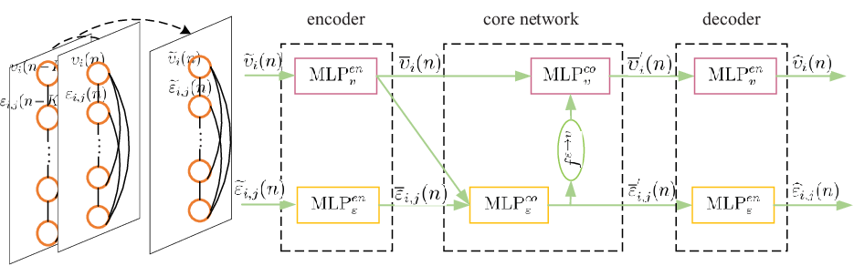
In order to track the massive MIMO channels, we design the GNN-based framework in Fig. 3. This architecture includes an encoder, a core network and a decoder. The historical channel samples are fed into the encoder to initialize the core network, the core network uses the graph structure to update nodes and edges, and the decoder independently decodes the edge and vertex attributes. The output of the decoder is $\mathcal{\widehat{G}}(n)$.

To better achieve the time-correlation of the massive MIMO channels, we combine the channel graph $\mathcal{G}(n)$ at the current time with the graph $\mathcal{G}(n-K)$ for the time $n-K$ to regenerate the graph $\widetilde{\mathcal{G}}(n)$ as the input of the encoder. Correspondingly, $\widetilde{\mathcal{G}}(n)$ can be denoted as

and its vertices $\widetilde{\bm{\upsilon}}_{i}(n)$ and edges $\widetilde{\bm{\varepsilon}}_{i,j}(n)$ can be expressed as

where ${\bm{\upsilon}}_{i}(n-K)$, ${\bm{\varepsilon}}_{i,j}(n-K)$ separately represent the vertex and the edge of $\mathcal{G}(n-K)$.

As well known, the DL performance is closely related with the feature representation. Thus, in our structure, we utilize the encoder part to extract and describe the latent features of $\mathcal{\tilde{G}}(n)$. Specifically, different multilayer perceptrons (MLPs) are resorted to independently extract the features of the vertices and edges in $\mathcal{\tilde{G}}(n)$. For $\widetilde{\bm{\varepsilon}}_{i,j}(n)$ and $\widetilde{\bm{\upsilon}}_{i}(n)$, the operations can be explicitly written as

where $\overline{\bm{\upsilon}}_{i}(n)$ and $\overline{\bm{\varepsilon}}_{i,j}(n)$ are the resultant features, while $\mathrm{MLP}_{\varepsilon}^{en}$ and $\mathrm{MLP}_{\upsilon}^{en}$ are the adopted MLPs during the encoder part.

Then, the graph $\overline{\mathcal{G}}(n)$ formed by $\overline{\bm{\upsilon}}_{i}(n)$, $\overline{\bm{\varepsilon}}_{i,j}(n)$ flows into the core network, which implements Algorithm 1 to achieve updated graph $\overline{\mathcal{G}}^{{}^{\prime}}(n)$. Different from the previous subsection, we utilize the MLP, i.e, $\mathrm{MLP}_{\varepsilon}^{co}$, to conduct $f^{\varepsilon}$, while $\mathrm{MLP}_{\upsilon}^{co}$ is used to fulfil $f^{\upsilon}$. Then, within this part, the three sub-functions of GN algorithm can be reexpressed as

In the decoder, we recover $\mathcal{\widehat{G}}(n)$ from $\mathcal{\bar{G}}^{{}^{\prime}}(n)$, where MLPs $\mathrm{MLP}_{v}^{de}$ and $\mathrm{MLP}_{e}^{de}$ are used for vertex $\overline{\bm{\upsilon}}_{i}^{{}^{\prime}}(n)$ and edge $\overline{\bm{\varepsilon}}_{i,j}^{{}^{\prime}}(n)$, respectively. Similarly, the process can be defined as

Finally, we reorganize the prediction output graph $\mathcal{\widehat{G}}(n)$ composed of $\widehat{\bm{\upsilon}}_{i}(n)$ and $\widehat{\bm{\varepsilon}}_{i,j}(n)$ to obtain $\widehat{\mathbf{h}}(n)$ as

where $[\widehat{\bm{\upsilon}}_{i}(n)]_{0}$ and $[\widehat{\bm{\upsilon}}_{i}(n)]_{1}$ represent the first and second elements of the $\widehat{\bm{\upsilon}}_{i}(n)$, respectively.

Our proposed channel scheme has two stages, i.e., the training and the deployment. In the first stage, we utilize the off-line learning scheme to train the GNN-based architecture to minimize the error between $\widehat{\mathbf{h}}(n)$ and $\mathbf{h}(n)$.

In the encoder and core network, for each MLP, we apply the same learning structure as shown in Fig. 4(a). Except for the output layer, the rectified linear unit (ReLU) activation function is utilized for each neuron. In addition, batch-normalization (BN) operation is utilized after the output layer to avoid gradient disappearance. The only difference between MLP in the encoder and that in the decoder is that the linear fully-connect (FC) layer with two output neurons is placed at the output of BN. The structure is shown in Fig. 4(b).

Without loss of generality, we use the mean square error (MSE) of the channel estimation as the loss function, and add the $L_{2}$-norm as the regularization function to improve the generalization ability. Therefore, the loss function can be written as

where $M_{tr}$ is the batch size, $\bm{\xi}$ are the weight parameters of MLPs to be learned, and $\kappa$ represents the regularization coefficient. The adaptive moment estimation (ADAM) [14] optimizer algorithm is adopted to achieve the optimal model parameters as $\bm{\xi}^{*}$.

In the on-line deployment stage, we load the trained parameters $\bm{\xi}^{*}$, pass the input data with the same structure as the training stage, and track the massive MIMO channels.

References

- [1] F. Rusek, D. Persson, B. K. Lau, E. G. Larsson, T. L. Marzetta, O. Edfors, and F. Tufvesson, “Scaling up MIMO: Opportunities and challenges with very large arrays,” IEEE Signal Process. Mag., vol. 30, no. 1, pp. 40–60, Jan. 2013.
- [2] J. Ma, S. Zhang, H. Li, N. Zhao, and V. C. M. Leung, “Interference-alignment and soft-space-reuse based cooperative transmission for multi-cell massive MIMO networks,” IEEE Trans. Commun., vol. 17, no. 3, pp. 1907–1922, Mar. 2018.
- [3] J. Ma, S. Zhang, H. Li, F. Gao, and S. Jin, “Sparse bayesian learning for the time-varying massive MIMO channels: Acquisition and tracking,” IEEE Trans. Commun., vol. 67, no. 3, pp. 1925–1938, Mar. 2019.
- [4] J. Zhao, F. Gao, W. Jia, J. Zhao, and W. Zhang, “Time varying channel tracking with spatial and temporal BEM for massive MIMO systems,” IEEE Trans. Commun., vol. 17, no. 17, pp. 5653–5666, Aug. 2018.
- [5] Y. Han, Q. Liu, C. Wen, M. Matthaiou, and X. Ma, “Tracking FDD massive MIMO downlink channels by exploiting delay and angular reciprocity,” IEEE J. Sel. Topics Signal Process., vol. 13, no. 5, pp. 1062–1076, Sep. 2019.
- [6] A. Al-Baidhani and H. H. Fan, ”Learning for detection: A deep learning wireless communication receiver over rayleigh fading channels,” in Proc. International Conference on Computing, Networking and Communications (ICNC), Honolulu, HI, USA, Feb. 2019, pp. 6-10.
- [7] X. Ma, H. Ye, and Y. Li, “Learning assisted estimation for time-varying channels,” in Proc. 15th International Symposium on Wireless Communication Systems (ISWCS), Lisbon, Aug. 2018, pp. 1–5.
- [8] C. Wen, W. Shih, and S. Jin, “Deep learning for massive MIMO CSI feedback,” IEEE Wireless Commun. Lett., vol. 7, no. 5, pp. 748–751, Oct. 2018.
- [9] Y. Yang, F. Gao, X. Ma, and S. Zhang, “Deep learning-based channel estimation for doubly selective fading channels,” IEEE Access, vol. 7, pp. 36 579–36 589, Feb. 2019.
- [10] C. Chun, J. Kang and I. Kim, ”Deep learning-dased joint pilot design and channel estimation for multiuser MIMO channels,” IEEE Commun. Lett., vol. 23, no. 11, pp. 1999–2003, Nov. 2019.
- [11] F. Scarselli, M. Gori, A. C. Tsoi, M. Hagenbuchner, G. Monfardini, “The graph neural network model,” IEEE Trans. Neural Networks., vol. 20, no. 1, pp. 61–80, Jan. 2009.
- [12] Z. Cui, K. Henrickson, R. Ke, and Y. Wang, “Temporal graph convolutional networks for traffic speed prediction considering external factors,” in Proc. 20th IEEE International Conference on Mobile Data Management (MDM), Hong Kong, Jun. 2019, pp. 234–242.
- [13] T. Song, S. R. Chowdhury, F. Yang, H. Jacobs, G. E. Fakhri, Q. Li, K. Johnson and J. Dutta, “Graph convolutional neural networks for alzheimer¡¯s disease classification,” in Proc. IEEE 16th International Symposium on Biomedical Imaging (ISBI), Venezia, Italy, Apr. 2019, pp. 414–417.
- [14] D. P. Kingma and J. Ba, “ADAM: A method for stochastic optimization,” arXiv:1412.6980, 2014. [Online]. Available: https://arxiv.org/abs/1412.6980