Phase equilibrium of liquid water and hexagonal ice from enhanced sampling molecular dynamics simulationsPreprint: AIP/123-QED
Abstract
We study the phase equilibrium between liquid water and ice Ih modeled by the TIP4P/Ice interatomic potential using enhanced sampling molecular dynamics simulations. Our approach is based on the calculation of ice Ih-liquid free energy differences from simulations that visit reversibly both phases. The reversible interconversion is achieved by introducing a static bias potential as a function of an order parameter. The order parameter was tailored to crystallize the hexagonal diamond structure of oxygen in ice Ih. We analyze the effect of the system size on the ice Ih-liquid free energy differences and we obtain a melting temperature of 270 K in the thermodynamic limit. This result is in agreement with estimates from thermodynamic integration (272 K) and coexistence simulations (270 K). Since the order parameter does not include information about the coordinates of the protons, the spontaneously formed solid configurations contain proton disorder as expected for ice Ih.
I Introduction
The study of phase equilibria using computer simulations is of central importance to understand the behavior of a given model. However, finding the thermodynamic condition at which two or more phases coexist is particularly hard in the presence of first order phase transitions. In this case, the transformation between phases takes place through nucleation and growth, and this mechanism is characterized by a free energy barrier. As a consequence of this barrier, transitions between the phases are rarely observed during a standard molecular dynamics simulation. This lack of ergodicity renders the estimation of the free energy difference between the phases involved impossible, except in trivial models.
Here we shall focus on the case of water. This ubiquitous and fascinating substance has at least 18 solid polymorphs that exhibit rich and diverse characteristics. The most stable form of ice at ambient pressure is ice Ih, and it is therefore the most common polymorph in planet Earth’s surface and atmosphere. In spite of the complexity of water, the phase diagram of many water models has been carefully studied using a combination of the thermodynamic integration technique and the integration of the Clausius-Clapeyron equation Sanz et al. 2004; Vega, Sanz, and Abascal 2005. The equilibrium between liquid water and ice Ih, in particular, has also been studied using the direct coexistence techniqueGarcía Fernández, Abascal, and Vega 2006; Conde, Rovere, and Gallo 2017 and the interface pinning methodPedersen et al. 2013; Cheng et al. 2019.
In this work we employ enhanced sampling simulations to study the equilibrium between liquid water and ice Ih. We used the TIP4P/IceAbascal et al. 2005 water model that considers rigid molecules. In order to achieve ergodic sampling, we construct a bias potential using the variational principle of Valsson and ParrinelloValsson and Parrinello 2014. The bias potential is a function of an order parameter designed to distinguish between the liquid phase and ice Ih. An important feature of this order parameter is that it drives the crystallization of ice Ih such that the crystal structure forms in an orientation compatible with the simulation boxPiaggi and Parrinello 2019.
II Crystal structure of ice Ih
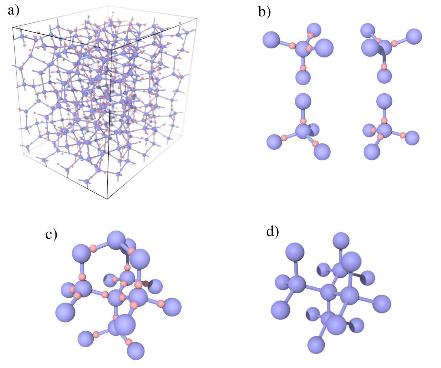
.
Before discussing the details of the order parameter we will describe the crystal structure of ice Ih Petrenko and Whitworth 1999 (see Fig. 1a). Ice Ih can be thought of as a lattice of oxygen atoms arranged in the hexagonal diamond crystal structure. In this crystal structure the basic environment around each oxygen atom has four oxygen neighbors arranged in a regular tetrahedron. The lattice has a 4 atom basis, therefore there are 4 distinct environments if the symmetry operations of the space group are not considered. In other words, in the crystal structure the basic environment can have 4 distinct orientations as shown in Fig. 1b. The basic environment is shared both in ice Ih and ice Ic, although these structures can be distinguished by considering extended environments (see Fig. 1c and d).
We now consider the positions of the hydrogen atoms (protons) within the hexagonal diamond lattice of oxygen. The positions of the protons will determine the orientation of the water molecules. Since the identity of the water molecule is preserved in ice Ih then the protons have to satisfy the ice rules proposed by Bernal and FowlerBernal and Fowler 1933 and stated clearly in ref. 13 by Pauling. The ice rules state that each oxygen atom has two nearest neighbor protons, with a distance similar to the one shown in the gas or the liquid phase, and two next nearest neighbor protons. Alternatively one can think that each oxygen-oxygen bond in the hexagonal diamond lattice has exactly one proton that is closer to one of the two oxygen atoms. Bernal and Fowler notedBernal and Fowler 1933, however, that this prescription does not completely determine the position of the protons in the lattice. Indeed, one of the most fascinating characteristics of ice Ih is that it contains proton disorder. The proton disorder gives rise to an entropic contribution to the free energy called residual entropy making the entropy of ice Ih at 0 K non-zero. PaulingPauling 1935 estimated the residual entropy of ice Ih to be per molecule and this result is often used as an input to the calculation of free energies of water using thermodynamic integrationVega, Sanz, and Abascal 2005.
It is worth noting that there is a proton ordered phase of ice in which the oxygen atoms sit in the same positions as in ice IhTajima, Matsuo, and Suga 1982. This phase is called ice XI and has a net polarization along the crystallographic axis. It is thus ferroelectric.
III On the order parameter for ice Ih
In this work, we aim to perform simulations that go reversibly from the liquid to ice Ih with arbitrary proton configurations. For this reason we will construct an order parameter that depends only on the position of the oxygen atoms. In this way, the proton configuration will form spontaneously during the simulation without any bias towards a particular configuration. We will employ the order parameter introduced in ref. 9 and we summarize here only the most important details.
We consider the four different extended environments of the hexagonal diamond lattice , and . One of these environments is shown in Fig. 1c and the rest of them correspond to rotations of the one shown. We also define a similarity kernelBartók, Kondor, and Csányi 2013 between with and a generic environment ,
| (1) |
where and are the atomic densities corresponding to the environments and , respectively. If the densities are represented by sums of Gaussians centered at the neighbors’ positions with spread , the kernel becomes:
| (2) |
where is the number of neighbors in the environment , and and are the positions of the neighbors in environments and , respectively. In Eq. (2) we have added a normalization such that . Now we have 4 similarity kernels that allow us to identify whether a given environment is compatible with one of the environments in ice Ih. However, we would like a single similarity measure between a given environment and any of the 4 environments in ice Ih. Thus we define another kernel,
| (3) |
that achieves that purpose.
Since there is one value of per oxygen atom, any given bulk configuration will have a distribution of this quantity. We show in Fig. 2 the distributions of in liquid water and in ice Ih at 270 K. The two distributions have a small overlap and therefore can be used to distinguish between liquid water and ice Ih environments. Here we have chosen the spread of the Gaussians such that the two distributions are approximately symmetrical with respect to . This will turn out useful below when we define a threshold between values of consistent with the liquid and those consistent with the solid. The rationale behind the choice of is the following. A large value of gives a more lenient definition of the target environment and thus shifts the distributions to the right. On the other hand, a small value of gives a too strict definition and thermal motion of atoms will create too large a deviation from the target environments. In this case the distributions are shifted to the left. In between these extremes one finds a value of that leads to distributions such as those shown in Fig. 2.
The similarity kernel defined in Eq. (3) provides a way to characterize the environments in a given configuration as being compatible with the environments in ice Ih. For a system with water molecules there will be oxygen-oxygen environments . We shall define two global order parameters. The first is the average value of the similarity kernel:
| (4) |
and the second is the number of environments consistent with the ice Ih environments,
| (5) |
where is a watershed between values of consistent with the liquid and those consistent with the solid.
According to our choice of a reasonable value of is .
The order parameter defined in Eq. (5) has to be made continuous and differentiable to be used in enhanced sampling simulations.
We refer the reader to section VIII for an appropriate definition of .
Equipped with these order parameters able to distinguish the liquid phase from ice Ih we shall now describe the enhanced sampling methodology.
IV Biased distribution of the order parameter
As discussed in the introduction, first order phase transitions are characterized by a free energy barrier. We anticipate some of the results and we plot in Fig. 3 the free energy as a function of the order parameter defined as,
| (6) |
where the marginal probability is,
| (7) |
is the inverse temperature, is the pressure, is the volume, is the potential energy, and is the appropriate partition function. For every temperature Fig. 3 shows two minima at and that correspond to the liquid and ice Ih. Furthermore, it shows that the barrier for the transformation is around 25-30 kT and therefore a standard molecular dynamics simulation cannot provide ergodic sampling. For this reason we aim at performing a simulation that samples a probability distribution different from that of the isothermal-isobaric ensemble. We choose to sample the so called well-tempered distributionBonomi and Parrinello 2010; Barducci, Bussi, and Parrinello 2008 of . This distribution is defined as,
| (8) |
where is known as bias factor. The effective free energy as a function of is then,
| (9) |
with an immaterial constant. The free energy barrier is thus reduced by the factor and we shall choose this parameter such that the barrier in is approximately kT. Consequently, we achieve ergodic sampling of the liquid and solid phases.
In order to sample the well-tempered distribution we introduce a bias potential that is a function of the order parameter. We shall calculate using a variational principleValsson and Parrinello 2014 such that the sampled distribution is . During an initial stage of the simulation we will optimize a set of variational coefficients until the distribution is sampled. Once this target distribution is reached we will fix the variational parameters and continue the simulation with a static bias potential . Further details can be found below in section VIII.
The first simulations carried out with this approach resulted in the crystallization of structures with misorientation and stacking faults. This had also been observed in ref. 9 and we employ the same strategy used in that work to avoid these structures. The strategy is based on the introduction of a bias potential that discourages these structures. Details can be found in section VIII.
V Calculation of free energy differences
We are now in a position to calculate the free energy difference between ice Ih and the liquid from the simulation described above. in the isothermal-isobaric ensemble at inverse temperature and pressure is defined as:
| (10) |
where . can be written using ensemble averages by introducing the Heaviside function,
| (11) |
where is some characteristic value of the order parameter that separates the liquid and ice Ih and thus,
| (12) |
Since the regions of high free energy do not contribute significantly to , the results of the calculations are not very sensitive to the choice of . A good and simple choice is .
Since the simulation was not performed in the isothermal-isobaric ensemble but rather in a biased one, the equation above has to be rewritten in terms of ensemble averages in the latter ensemble. Thus,
| (13) |
where are the weights associated to the bias potentials acting on the system, and denotes an ensemble average in the biased ensemble. This is the equation that we shall use to calculate from the simulations.
VI Results
We now turn to discuss the results of the calculations. We performed simulations with three different system sizes composed of 16, 96, and 288 water molecules. We studied temperatures from 270 K to 300 K based on previous reports of the melting temperature of ice Ih described by the TIP4P/Ice potentialGarcía Fernández, Abascal, and Vega 2006; Abascal et al. 2005. We show in Figure 3 the free energy defined in Eq. (6) as a function of temperature for the system of 96 water molecules. At 270 K ice Ih is more stable than the liquid but the stability is reversed at 280 K and above. As previously mentioned, the free energy barriers are around 25-30 kT.
In Fig. 4a we plot as a function of simulation time at different temperatures. The figure shows that the number of transitions from the liquid to the solid per unit time decreases as the temperature is lowered. In order to quantify this effect we calculated for each temperature the time autocorrelation function of ,
| (14) |
where and we have used to emphasize that the average was done using the biased trajectories. We plot in Figure 4b. We also fitted a decaying exponential function to in order to calculate a characteristic correlation time . Figure 4c shows as a function of temperature and from this plot we see that the autocorrelation time increases exponentially as the temperature is lowered. Note that these are not the system’s physical autocorrelation times but those of the system under the influence of the bias potential.
The phenomenon described in the previous paragraph bears some resemblance to the critical slowing down found in Monte Carlo simulations of lattice models and typically characterized with a dynamical exponentNewman and Barkema 1999. However, the situation here is different since the slowing down is most likely a result of a rough free energy landscape in directions orthogonal to our order parameter that gives rise to glass-like behavior. We ruled out the possibility that this behavior is a consequence of lack of convergence of the bias potential by plotting the biased free energy as a function of for each temperature. The barriers found ranged from 1.5 to 3 kT and therefore cannot be responsible of the behavior shown in Fig. 4. Furthermore, this phenomenon has also been observed for another glass former, namely silicaNiu et al. 2018. A possible way to address this issue is the parallel temperingHansmann 1997; Sugita and Okamoto 1999 technique or the approach outlined in ref. 22.
We now set out to study the finite size effects in the melting temperature of ice Ih. For this purpose we repeated the calculations described above using 16 and 288 water molecules instead of 96. Then, we calculated the free energy differences using Eq. (13). The results thus obtained are shown in Fig. 5a where we plot vs. inverse system size at four different temperatures. We also report in Table 1. From the data at each temperature we extrapolated the results to . scales linearly with as predicted by the theory of finite size scaling in first order phase transitionsBinder 1987.
We then proceed to plot vs. temperature in Fig. 5b including the results of the extrapolation to the thermodynamic limit described in the previous paragraph. By fitting a straight line to the results in the thermodynamic limit we obtain our best estimate of the melting temperature which is . We summarize in Table 2 the results obtained using different methods.
| Temperature (K) | (NkT) | Temperature (K) | (NkT) |
|---|---|---|---|
| 16 molecules | 288 molecules | ||
| 270 | -0.29(3) | ||
| 280 | -0.20(3) | 280 | 0.068(1) |
| 290 | -0.150(8) | 290 | 0.15(1) |
| 300 | -0.093(5) | 300 | 0.24(1) |
| 96 molecules | molecules | ||
| 270 | -0.053(5) | 270 | -0.006(8) |
| 280 | 0.037(5) | 280 | 0.084(7) |
| 290 | 0.123(5) | 290 | 0.175(5) |
| 300 | 0.200(5) | 300 | 0.257(5) |
| Method | Melting temperature (K) |
|---|---|
| This work | 270(2) |
| Hamiltonian Gibbs-Duhem integration Vega, Sanz, and Abascal 2005; Abascal et al. 2005 | 272(6) |
| CoexistenceGarcía Fernández, Abascal, and Vega 2006 | 268(2) |
| CoexistenceConde, Rovere, and Gallo 2017 | 269.8(1) |
| Free surfaceVega, Martin-Conde, and Patrykiejew 2006 | 271(1) |
| Experimental | 273.15 |

The agreement between our method and thermodynamic integrationVega, Sanz, and Abascal 2005; Abascal et al. 2005 is remarkable if one takes into account that the latter requires as input the entropic contribution of the proton disorder. Instead, in our method the proton configuration appears spontaneously during crystallization and there is no explicit bias because the order parameter is only a function of the positions of oxygen atoms. Below we analyze the proton configurations obtained from our simulations.
The proton configuration will determine the total dipole moment of the system. We will thus use the dipole moment per molecule, , where is the dipole moment versor of molecule and is the number of molecules, to analyze the proton configuration. We note that in the equation above we assume the dipole moment of each molecule to be one. Since the molecules are rigid, using a different value would not change our results qualitatively. In Fig. 6a we plot a 2D histogram of the projection of along two directions. The x-axis is the direction perpendicular to the prismatic plane and the y-axis is the direction perpendicular to the basal plane . We also show in Figs. 6b and c the 1D histograms along the same directions described in Fig. 6a. In these Figures we compare the results for liquid water (blue) and ice Ih (orange) for a system of water molecules at 300 K. Both distributions are centered at as expected for non-ferroelectric phases like liquid water and ice Ih. Therefore our configurations are compatible with the criterion used by Rahman and Stillinger to construct proton disordered configurationsRahman and Stillinger 1972. The distribution of in water can be well described by a multivariate normal distribution. On the other hand, the distribution of in ice Ih shows several peaks that form a lattice. This is expected since the crystal structure of the oxygen atoms allows only a restricted number of directions for the dipole moment (6 in each environment).
In Fig. 6 we also show for the proton ordered phase, i.e. ice XI. The configurations obtained during the simulations are far away from the ordered configurations and are also centered at . This suggests that our configurations are representative of the proton disorder in ice Ih.
We also plot the distribution of the norm in Fig. 6d. The distribution of the liquid is very similar to the Maxwell-Boltzmann distribution as follows from the fact that has a multivariate normal distribution. The distribution of ice Ih also resembles the Maxwell-Boltzmann distribution although there are some anomalous peaks. Rahman and StillingerRahman and Stillinger 1972 found a smoother distribution for a larger system and it is reasonable to think that in the thermodynamic limit the multiple peaks in our histogram would also be absent. Indeed, we repeated our analysis for the system with molecules and found an increase in the number of peaks that are also closer to each other.
VII Conclusions
We have calculated the melting temperature of ice Ih as described by the TIP4P/Ice water model using enhanced sampling molecular simulations. Our best estimate of the melting temperature is 270 K in the thermodynamic limit. This result agrees with previous estimates that put the melting temperature between 268 and 272 K. Therefore the results show that enhanced sampling simulations offer a state-of-the-art alternative to calculating melting temperatures and differences in free energy between the liquid and the solid.
A key feature of this approach is the use of an order parameter that enforces a particular orientation of the crystal structure. The order parameter is based on a measure of the similarity between the atomic environments in a given configuration and reference environments. The reference environments were chosen in order to obtain the crystal structure of ice Ih and included 17 nearest neighbors.
We argue that there are several advantages to our approach. For one, since the crystallization and melting processes are explicitly simulated, physical insight can be extracted directly from these simulations. For instance, we could initially observe stacking faults that point to the competition between ice Ih and ice Ic. We later improved our simulation setup in order to avoid this phenomenon and obtained only ice Ih. In addition, our results automatically include the effects of proton disorder. Our order parameter does not include any information about the orientation of the water molecules and therefore it does not bias the structure towards any particular proton configuration.
We also observed an exponentially slower sampling as the temperature is decreased. This is surprising if one considers that the free energy as a function of the order parameter has been flattened. We suggest that this result is a consequence of a rough free energy landscape in directions orthogonal to our order parameter. This observation would be compatible with the tendency of water to form glasses.
VIII Computational details
The simulations were carried out using LAMMPSPlimpton 1995 patched with the PLUMED 2Tribello et al. 2014 enhanced sampling plugin. PLUMED 2 was supplemented with the VES moduleves. The input files to reproduce all simulations are available on the PLUMED-NESTBonomi et al. 2019 as part of a collective effort to improve the transparency and reproducibility of enhanced molecular simulations. We employed a timestep for the integration of the equations of motion of 2 fs in all simulations. The temperature was controlled using the stochastic velocity rescaling algorithmBussi, Donadio, and Parrinello 2007 with a 0.1 ps relaxation time. The pressure was maintained at 1 bar using an isotropic version of the Parrinello-Rahman barostatParrinello and Rahman 1981 with a 1 ps relaxation time. The bond lengths and angles were kept fixed using the SHAKE algorithmRyckaert, Ciccotti, and Berendsen 1977. A cutoff of 0.85 nm was used for the Lennard-Jones and Coulomb interactions. Long-range Coulomb interactions beyond this cutoff were computed with the particle-particle particle-mesh (PPPM) solverHockney and Eastwood 1988. Tail corrections to the pressure and energy were included to take into account long-range effects neglected due to the Lennard-Jones potential truncationFrenkel and Smit 2001.
The bias potential was constructed using the variational principle of Valsson and ParrinelloValsson and Parrinello 2014 that we summarize below. Within this formalism, the bias potential is determined through the minimization of the functional,
| (15) |
where is a set of collective variables (CVs) that are a function of the atomic coordinates , the free energy is given within an immaterial constant by , is the interatomic potential, and is a preassigned target distribution. The minimum of this convex functional is reached for:
| (16) |
which amounts to saying that in a system biased by , the distribution of the CVs is .
As described in the main part, we used as CV and we targeted the so called well-tempered distributionValsson and Parrinello 2015, i.e. . We employed bias factors of 30, 50, and 100 for the systems of 16, 96, and 288 molecules, respectively. The bias potential was expanded in Legendre polynomials of order 20 defined in the interval . The functional was minimized using the averaged stochastic gradient descent algorithmValsson and Parrinello 2014; Bach and Moulines 2013 and the gradient was averaged over 500 timesteps. The step size in the optimization was 2 kJ/mol. The well-tempered distribution was determined self-consistently as described in ref. 35 with update frequency 100 optimization iterations. Four multiple walkersRaiteri et al. 2006 contributed to the statistics to calculate the gradient of . Once the bias potential was deemed converged the optimization was stopped and the simulation was continued with a static bias potential akin to the ones employed in the umbrella sampling techniqueTorrie and Valleau 1977. All the reported quantities were calculated under the action of a static bias potential.
The order parameters in Eqs. (4) and (5) require the specification of the environments and the spread of the Gaussians . We employed , , for the systems of ,, molecules, respectively. In Eq. (5) we defined an order parameter that counts the number of molecules that satisfy where is chosen to be . However, the definition given above cannot be used in enhanced sampling simulations since it is not continuous and differentiable. For this reason in the simulations we employed the following expressionTribello et al. 2017,
| (17) |
with and for the 96 molecule case, and and for the 96 and 288 molecule cases. In the limit of large and Eqs. (5) and (17) yield the same result. By the same token, Eq. (3) cannot be used in enhanced sampling simulations. A continuous and differentiable variant of Eq. (3) is,
| (18) |
where was chosen, and the index runs over the 4 local environments of ice Ih. This is the expression we have used in the simulations. For , Eq. (18) selects the largest with .
As described above, we added bias potentials to discourage the formation of structures with misorientation or stacking faults. For this purpose we defined two collective variables. The first aims at distinguishing structures misaligned with respect to the box as is defined as,
| (19) |
where is the global Steinhardt parameterSteinhardt, Nelson, and Ronchetti 1983 as defined in ref. 41 and is defined in Eq. (4). The superscripts in Eq. (19) refer to the values of the order parameters in the liquid () and in ice Ih (). The rationale behind has been described in ref. 9. On the other hand, the purpose of the second collective variable is to distinguish perfect structures from those with stacking faults. It is defined as,
| (20) |
where the symbols with the subscript refer to the kernel defined for the cubic diamond structure.
In the simulations and/or were restrained with harmonic potentials,
| (21) |
and the chosen and for each simulation can be found in the simulation input files made available.
Acknowledgements.
P.M.P thanks Marcos Calegari for useful discussions and Zachary Goldsmith for carefully reading the manuscript. P.M.P was supported by an Early Postdoc.Mobility fellowship from the Swiss National Science Foundation. This work was conducted within the center: Chemistry in Solution and at Interfaces funded by the DoE under Award DE-SC0019394. The calculations reported in this work were performed using the Princeton Research Computing resources at Princeton University.Data Availability Statement
The input files and results of the simulations are openly available on GitHubPiaggi 2020, and on PLUMED-NEST (www.plumed-nest.org), the public repository of the PLUMED consortiumBonomi et al. 2019, as plumID:20.010.
References
- Sanz et al. (2004) E. Sanz, C. Vega, J. Abascal, and L. MacDowell, “Phase diagram of water from computer simulation,” Physical review letters 92, 255701 (2004).
- Vega, Sanz, and Abascal (2005) C. Vega, E. Sanz, and J. Abascal, “The melting temperature of the most common models of water,” The Journal of chemical physics 122, 114507 (2005).
- García Fernández, Abascal, and Vega (2006) R. García Fernández, J. L. Abascal, and C. Vega, “The melting point of ice Ih for common water models calculated from direct coexistence of the solid-liquid interface,” The Journal of chemical physics 124, 144506 (2006).
- Conde, Rovere, and Gallo (2017) M. Conde, M. Rovere, and P. Gallo, “High precision determination of the melting points of water tip4p/2005 and water tip4p/ice models by the direct coexistence technique,” The Journal of chemical physics 147, 244506 (2017).
- Pedersen et al. (2013) U. R. Pedersen, F. Hummel, G. Kresse, G. Kahl, and C. Dellago, “Computing gibbs free energy differences by interface pinning,” Physical Review B 88, 094101 (2013).
- Cheng et al. (2019) B. Cheng, E. A. Engel, J. Behler, C. Dellago, and M. Ceriotti, “Ab initio thermodynamics of liquid and solid water,” Proceedings of the National Academy of Sciences 116, 1110–1115 (2019).
- Abascal et al. (2005) J. Abascal, E. Sanz, R. García Fernández, and C. Vega, “A potential model for the study of ices and amorphous water: Tip4p/ice,” The Journal of chemical physics 122, 234511 (2005).
- Valsson and Parrinello (2014) O. Valsson and M. Parrinello, “Variational approach to enhanced sampling and free energy calculations,” Physical review letters 113, 090601 (2014).
- Piaggi and Parrinello (2019) P. M. Piaggi and M. Parrinello, “Calculation of phase diagrams in the multithermal-multibaric ensemble,” The Journal of chemical physics 150, 244119 (2019).
- Stukowski (2009) A. Stukowski, “Visualization and analysis of atomistic simulation data with ovito–the open visualization tool,” Modelling and Simulation in Materials Science and Engineering 18, 015012 (2009).
- Petrenko and Whitworth (1999) V. F. Petrenko and R. W. Whitworth, Physics of ice (OUP Oxford, 1999).
- Bernal and Fowler (1933) J. D. Bernal and R. H. Fowler, “A theory of water and ionic solution, with particular reference to hydrogen and hydroxyl ions,” The Journal of Chemical Physics 1, 515–548 (1933).
- Pauling (1935) L. Pauling, “The structure and entropy of ice and of other crystals with some randomness of atomic arrangement,” Journal of the American Chemical Society 57, 2680–2684 (1935).
- Tajima, Matsuo, and Suga (1982) Y. Tajima, T. Matsuo, and H. Suga, “Phase transition in koh-doped hexagonal ice,” Nature 299, 810–812 (1982).
- Bartók, Kondor, and Csányi (2013) A. P. Bartók, R. Kondor, and G. Csányi, “On representing chemical environments,” Physical Review B 87, 184115 (2013).
- Bonomi and Parrinello (2010) M. Bonomi and M. Parrinello, “Enhanced sampling in the well-tempered ensemble,” Physical review letters 104, 190601 (2010).
- Barducci, Bussi, and Parrinello (2008) A. Barducci, G. Bussi, and M. Parrinello, “Well-tempered metadynamics: A smoothly converging and tunable free-energy method,” Physical review letters 100, 020603 (2008).
- Newman and Barkema (1999) M. Newman and G. Barkema, Monte carlo methods in statistical physics chapter 1-4 (Oxford University Press: New York, USA, 1999).
- Niu et al. (2018) H. Niu, P. M. Piaggi, M. Invernizzi, and M. Parrinello, “Molecular dynamics simulations of liquid silica crystallization,” Proceedings of the National Academy of Sciences 115, 5348–5352 (2018).
- Hansmann (1997) U. H. Hansmann, “Parallel tempering algorithm for conformational studies of biological molecules,” Chemical Physics Letters 281, 140–150 (1997).
- Sugita and Okamoto (1999) Y. Sugita and Y. Okamoto, “Replica-exchange molecular dynamics method for protein folding,” Chemical physics letters 314, 141–151 (1999).
- Yang, Niu, and Parrinello (2018) Y. I. Yang, H. Niu, and M. Parrinello, “Combining metadynamics and integrated tempering sampling,” The Journal of Physical Chemistry Letters 9, 6426 (2018).
- Binder (1987) K. Binder, “Theory of first-order phase transitions,” Reports on progress in physics 50, 783 (1987).
- Vega, Martin-Conde, and Patrykiejew (2006) C. Vega, M. Martin-Conde, and A. Patrykiejew, “Absence of superheating for ice ih with a free surface: A new method of determining the melting point of different water models,” Molecular Physics 104, 3583–3592 (2006).
- Rahman and Stillinger (1972) A. Rahman and F. H. Stillinger, “Proton distribution in ice and the kirkwood correlation factor,” The Journal of Chemical Physics 57, 4009–4017 (1972).
- Plimpton (1995) S. Plimpton, “Fast parallel algorithms for short-range molecular dynamics,” Journal of computational physics 117, 1–19 (1995).
- Tribello et al. (2014) G. A. Tribello, M. Bonomi, D. Branduardi, C. Camilloni, and G. Bussi, “Plumed 2: New feathers for an old bird,” Computer Physics Communications 185, 604–613 (2014).
- (28) VES Code, a library that implements enhanced sampling methods based on Variationally Enhanced Sampling written by O. Valsson. For the current version, see http://www.ves-code.org.
- Bonomi et al. (2019) M. Bonomi, G. Bussi, C. Camilloni, G. A. Tribello, P. Banáš, A. Barducci, M. Bernetti, P. G. Bolhuis, S. Bottaro, D. Branduardi, et al., “Promoting transparency and reproducibility in enhanced molecular simulations,” Nature methods 16, 670–673 (2019).
- Bussi, Donadio, and Parrinello (2007) G. Bussi, D. Donadio, and M. Parrinello, “Canonical sampling through velocity rescaling,” The Journal of chemical physics 126, 014101 (2007).
- Parrinello and Rahman (1981) M. Parrinello and A. Rahman, “Polymorphic transitions in single crystals: A new molecular dynamics method,” Journal of Applied physics 52, 7182–7190 (1981).
- Ryckaert, Ciccotti, and Berendsen (1977) J.-P. Ryckaert, G. Ciccotti, and H. J. Berendsen, “Numerical integration of the cartesian equations of motion of a system with constraints: molecular dynamics of n-alkanes,” Journal of computational physics 23, 327–341 (1977).
- Hockney and Eastwood (1988) R. W. Hockney and J. W. Eastwood, Computer simulation using particles (crc Press, 1988).
- Frenkel and Smit (2001) D. Frenkel and B. Smit, Understanding molecular simulation: from algorithms to applications, Vol. 1 (Academic press, 2001).
- Valsson and Parrinello (2015) O. Valsson and M. Parrinello, “Well-tempered variational approach to enhanced sampling,” Journal of chemical theory and computation 11, 1996–2002 (2015).
- Bach and Moulines (2013) F. Bach and E. Moulines, “Non-strongly-convex smooth stochastic approximation with convergence rate o (1/n),” in Advances in Neural Information Processing Systems (2013) pp. 773–781.
- Raiteri et al. (2006) P. Raiteri, A. Laio, F. L. Gervasio, C. Micheletti, and M. Parrinello, “Efficient reconstruction of complex free energy landscapes by multiple walkers metadynamics,” The Journal of Physical Chemistry B 110, 3533–3539 (2006).
- Torrie and Valleau (1977) G. M. Torrie and J. P. Valleau, “Nonphysical sampling distributions in monte carlo free-energy estimation: Umbrella sampling,” Journal of Computational Physics 23, 187–199 (1977).
- Tribello et al. (2017) G. A. Tribello, F. Giberti, G. C. Sosso, M. Salvalaglio, and M. Parrinello, “Analyzing and driving cluster formation in atomistic simulations,” Journal of chemical theory and computation 13, 1317–1327 (2017).
- Steinhardt, Nelson, and Ronchetti (1983) P. Steinhardt, D. Nelson, and M. Ronchetti, “Bond-orientational order in liquids and glasses,” Phys. Rev. B 28, 784–805 (1983).
- Van Duijneveldt and Frenkel (1992) J. Van Duijneveldt and D. Frenkel, “Computer simulation study of free energy barriers in crystal nucleation,” The Journal of chemical physics 96, 4655–4668 (1992).
- Piaggi (2020) P. Piaggi, “https://github.com/pablopiaggi/crystallization-of-iceih,” (2020).