Dynamical -boson stars: generic stability and evidence for non-spherical solutions
Abstract
-boson stars are static, spherical, multi-field self-gravitating solitons. They are asymptotically flat, finite energy solutions of Einstein’s gravity minimally coupled to an odd number of massive, complex scalar fields. A previous study assessed the stability of -boson stars under spherical perturbations, finding that there are both stable and unstable branches of solutions, as for single-field boson stars (). In this work we probe the stability of -boson stars against non-spherical perturbations by performing numerical evolutions of the Einstein-Klein-Gordon system, with a 3D code. For the timescales explored, the -boson stars belonging to the spherical stable branch do not exhibit measurable growing modes. We find, however, evidence of zero modes; that is, non-spherical perturbations that neither grow nor decay. This suggests the branching off towards a larger family of equilibrium solutions: we conjecture that -boson stars are the enhanced isometry point of a larger family of static (and possibly stationary), non-spherical multi-field self-gravitating solitons.
pacs
04.25.D-, 95.30.Sf 95.35.+dI Introduction
Boson stars Kaup68; Ruffini69 (see Schunck:2003kk; Liebling:2012fv for reviews) are remarkable gravitational solitons. These self-gravitating, localised energy lumps of a complex, massive scalar field have appealing theoretical properties. A key one is their dynamical stability. For spherical boson stars there is a stable branch of solutions against perturbations. Indeed, a variety of studies including linear perturbation theory 1989NuPhB.315..477L; Gleiser:1988rq; Gleiser:1989a, catastrophe theory Kusmartsev:1991pm and numerical simulations Hawley2000; Seidel90; Guzman09; sanchis2017numerical; di2018dynamical agree that boson stars are perturbatively stable, as long as the amplitude of the scalar field is smaller than a critical value. When the latter is attained, boson stars acquire their maximum mass.
Being dynamically stable legitimates inquiring about the possible (astro)physical role of boson stars. Albeit exotic, lacking undisputed observational evidence, boson stars have found important applications in strong gravity and astrophysics. For instance, boson stars provide a common model for a black hole mimicker Mielke:2000mh; Torres2000; Guzman:2009zz; Olivares:2018abq. Being dynamically tractable, one can then compare dynamical spacetime properties, such as waveforms of binary boson star systems, with those of black holes Palenzuela:2006wp; Palenzuela:2007dm; bezares2017final. This is particularly timely in view of the recently initiated gravitational-wave astronomy era Abbott:2016blz; TheLIGOScientific:2016qqj, which provides data for both models to be compared with.
A second important application is in relation to a central mystery of contemporary science: the nature of dark matter. An increasing attention has been dedicated to models that consider dark matter as an ultra-light bosonic particle Matos:1999et; Matos:2000ss; Hu:2000ke; Hui:2016ltb. The bosonic nature allows this sort of dark matter to form coherent macroscopic excitations. In this context, bosons stars can model, in particular, the core of dark matter galactic halos Lee:1995af; Bernal:2009zy; UrenaLopez:2010ur; Schive:2014dra.
In their original guise, the Einstein-Klein-Gordon (EKG) model contains a massive, free scalar field, and the solitonic solutions are called mini-boson stars. A variety of generalisations ensued. Boson stars for scalar field theories with self-interactions have been reported, starting with the case of quartic self-interactions considered by Colpi et al. Colpi86. Spacetime angular momentum was introduced for mini-boson stars in Yoshida:1997qf; Schunck:1996he, giving rise to stationary (but not static) self-gravitating solitons. A cousin model with a complex, massive vector (rather than scalar) field yields Proca stars brito2016proca. These and other examples use single (complex) field models; however, multi-field boson stars have also been reported. One example is given by multi-state boson stars Bernal:2009zy; UrenaLopez:2010ur; Li:2019mlk. More recently, multi-field boson stars with an arbitrary odd number, , , of equal mass, uncoupled (except through gravity) complex scalar fields with harmonic time dependence were introduced Alcubierre:2018ahf; they are dubbed -boson stars and they will be the focus of this paper.
-boson stars are described by spherically symmetric and static metrics. For they are simply the usual mini-boson stars. For , the scalar fields have an angular dependence given by the corresponding spherical harmonics . Then, if the radial dependence for all fields is the same, corresponding to choosing the amplitude of the spherical harmonics equal at all radial distances, static, spherical configurations are obtained, regardless of the energy-momentum tensor of each individual field being angular dependent. This is an example of symmetry non-inheritance: the (spherical) spacetime and the (non-spherical) individual matter fields do not share spherical symmetry. The usual boson stars already have a version of symmetry non-inheritance: the (time oscillating) scalar field and the (static) spacetime do not share time-translation symmetry. Consistency requires only that the spacetime geometry and the total energy-momentum tensor share the same symmetries, not the individual matter fields.
Generic -boson stars have been shown to exhibit similar properties to those of the standard stars. In particular, - boson stars have a stable branch of solutions against spherical perturbations Alcubierre:2019qnh. The main goal of this paper is to assess the stability of -boson stars (in this branch) against generic, non-spherical perturbations. As we shall see, our analysis will show that, in this respect, generic -boson star do not exactly mimic the case. Although no instabilities are observed, the analysis provides a glimpse of a larger landscape of solutions, of which -boson stars are just the enhanced symmetry point.
Departure from spherical symmetry is physically relevant. Firstly, spherical objects – such as -boson stars – need to be stable against non-spherical perturbations, in order to be dynamically viable. Secondly, astrophysical bodies are not, typically, perfectly spherical, in particular due to angular momentum. So one must assess if some perturbations actually deform -boson stars into acquiring new degrees of freedom. In this respect, it was recently proposed that multi-field boson stars, in the non-relativistic regime, could have non-spherical stable configurations guzman2019gravitational. This provides an extra motivation to inquire about the behaviour of relativistic -boson stars under non-spherical perturbations Finally, assessing non-spherical configurations and perturbations often yields a richer phenomenology. As a fruitful example, it was recently found that spinning, single-field mini-boson stars are unstable against non-axisymmetric perturbations, either decaying into a non-rotating boson star or collapsing into a Kerr black hole bezares2017final; sanchis2019nonlinear. By contrast, spinning Proca stars do not present instabilities under non-axisymmetric perturbations and furthermore, they can form dynamically sanchis2019nonlinear. This example shows how the study on non-spherical perturbations unveiled a new relevant dynamical property of boson stars.
We shall investigate the behaviour of -boson stars under non-spherical perturbations using fully non-linear numerical simulations of the corresponding Einstein-Klein-Gordon system. As initial data, we use configurations found in Alcubierre:2018ahf which are then perturbed in two different ways. The first type of perturbation tests the stability against non-axially symmetric perturbations, targeting potential bar-mode instabilities. The second type of perturbation tests the stability against a relative change in the amplitude of the internal fields. In none of the two cases measurable growing modes were found, either by perturbing the total mass density or by perturbing each of the constituent fields, as long the -boson star belongs to the stable branch against spherical perturbations. By following the evolution of distortion parameters (defined below) we found, however, evidence for long-lived perturbations, which we interpret as zero modes. These modes, in turn, are interpreted as evidence for a larger family of equilibrium solutions.
Consider the Schwarzschild black hole of vacuum General Relativity. It has been shown to be mode stable in the renowned works of Regge and Wheeler Regge57 and Zerilli Zerilli70. No gravitational perturbations grow. However, a perturbation that carries angular momentum yield not decay. The Schwarzschild solution migrates to a small angular momentum Kerr solution and oscillates around this new ground state. Similarly, a perturbation which electric charge will not decay and the spacetime will oscillate around a small charge Reissner-Nordström solution. These special perturbations are zero modes. Such modes are often found when a spacetime is unstable against some sort of perturbations, at the threshold between stable and unstable modes. An example occurs for the superradiant instability of the Kerr spacetime due to a massive bosonic field. The zero modes indicate the bifurcation of the Kerr family towards a new family of black holes with bosonic hair Herdeiro:2014goa; Herdeiro:2016tmi. But zero modes can also occur even if there is no instability, as in the Schwarzschild example, indicating, nonetheless, an enlarged family of solutions (Kerr or Reissner-Nordström), of which the initial spacetime (Schwarzschild) is a special case. Thus, one of the outcomes of our analysis is the conjecture that -boson stars are the enhanced isometry point of a larger family of static (and possibly stationary), non-spherical multi-field self-gravitating solitons.
In the rest of this work we will focus on configurations with . Such -boson stars are described by fields, with respectively. In order to follow the dynamics of the perturbed system a numerical code that solves the Einstein--Klein-Gordon system is required. We have used the Einstein Toolkit framework EinsteinToolkit:web; loffler2012f; Zilhao:2013hia with the Carpet package Schnetter:2003rb; CarpetCode:web for mesh-refinement capabilities to achieve our goal.
As a technical step we perform a Cauchy (3+1) decomposition on each scalar field that constitutes the star and solve the full Einstein--Klein-Gordon system. This is done implementing an arrangement in the Einstein Toolkit, a thorn, to solve scalar fields using finite differences sanchis2019nonlinear.
This paper is organized as follows: Section II addresses the construction of initial data to set up perturbed -boson stars. Section III describes the diagnostic tools used to monitor the evolution and some aspects used to decide on whether instabilities are present. The numerical results are described in Section IV and in Section V our conclusions and final remarks are presented. In this work we use units where .
II Initial Data
Following previous works on -boson stars
Alcubierre:2018ahf; Alcubierre:2019qnh, we consider a set of complex scalar fields, with mass and no self-interaction within the Einstein theory of gravity, for which the energy-momentum tensor is given by:
| (1) |
where the index labels each field and the stress-energy-momentum for each field is given by
| (2) | |||||
Complex conjugation is denoted by ‘*’. Following Olabarrieta:2007di; Alcubierre:2018ahf we propose a set of scalar fields of the form
| (3) |
where the angular momentum number is fixed, and , which plays the role of index in equation (3), takes the values (hence the total number of fields needed for a fixed value of will be ), are the spherical harmonics defined over the unitary 2D-sphere. Then we assume that the amplitudes are the same for all . It was shown in Alcubierre:2018ahf that if the fields have all the same amplitude , the stress-energy tensor (1) has spherical symmetry regardless if the fields have angular dependence. See also Olabarrieta:2007di and for a detailed discussion on the procedure, see Carvente:2019gkd.
Assuming the harmonic time dependence
| (4) |
where and the frequency are both real-valued, the stress-energy tensor becomes time independent. Under these assumptions it is possible to find self gravitating static, spherically symmetric equilibrium configurations by solving the EKG system of equations. Those configurations are parametrized by the angular momentum number , hence the name, -boson stars.
In order to obtain initial data suitable for numerical evolution, we construct equilibrium -boson stars, to be subsequently perturbed. Considering a spherically symmetric spacetime with a line element given by:
| (5) |
where and , are functions of , and the assumptions mentioned above for , the EKG system yields
| (6) | |||||
| (7) | |||||
| (8) | |||||
By studying the Klein-Gordon equation in the vicinity of one finds that the scalar field behaves as in that region. For a fixed value of the angular momentum number , a given value of the parameter , and the boundary condition at infinity requesting that decays exponentially, the system of equations (6-8) becomes a nonlinear eigenvalue problem for the frequency . We solve this set of equations in a finite size grid by means of a shooting method using the frequency as the shooting parameter. For numerical purposes we take the mass parameter .
Fig. 1 shows a plot of the Arnowitt-Deser-Misner (ADM) mass versus the frequency for the -boson stars. In Ref. Alcubierre:2018ahf it was shown that -boson stars with have similar properties to those of single-field mini-boson stars, the case. For instance, given a value of , the mass of the equilibrium configurations as a function of has a maximum, which gets larger as increases, yielding more compact stars. Furthermore, as in the case of -boson stars, the maximum value of the mass separates the space of solutions into two branches. These branches correspond to stable and unstable configurations against spherical perturbations, as shown in Alcubierre:2019qnh.
As mentioned above, the hypothesis that all the fields must have the same amplitude is essential to keep the spherical symmetry of the configuration. If one wants to consider different amplitudes of each constituent field, the assumption of spherical symmetry has to be relaxed. However, hitherto there has been no evidence that the resulting states may be equilibrium solutions of the Einstein--Klein-Gordon system. In this work we will show that deviations from spherical symmetry may indeed lead to new equilibrium solutions.

To proceed further with our non-spherical analysis we transform the solutions of the previous system of equations to Cartesian coordinates, . Then we perform a full non-linear numerical evolution of the perturbed stationary solutions.
III Diagnostics
In order to test the stability of the static solutions we perform two different types of perturbations:
(i) The first type consists in perturbing the energy density of the star given by , where is the four velocity of Eulerian observers in the 3+1 space time decomposition. The perturbed energy density is obtained by adding a non spherically symmetric small amplitude term to the homogeneous density in the following way Saijo:2000qt:
| (9) |
where is the energy density of the equilibrium configuration, obtained from the solution of Eqs. (6)-(8), and is the radius enclosing 99% of the configuration’s mass. In our simulations we choose . This type of perturbations could trigger a potential bar-mode instability because it only affects the and components of the quadrupole moment defined as
| (10) |
Since the value of is small , this perturbation can be considered linear, initially; more importantly, it breaks the spherical symmetry of the original solution.
(ii) The second type of perturbations consist in varying separately the amplitude of each field. With these perturbations it is possible to study the stability of the stars against variations on each mode and break the spherical symmetry. We choose the following form
| (11) |
where is the unperturbed solution of the system of Eqs. (6)-(8). This perturbation introduces an additional constraint violation, besides the well known numerical error, but its magnitude is controlled by choosing a small , which, in general, depends on the -mode. Note that if is the same for all , the perturbation is spherical.
In order to assess the stability properties of the stars during the numerical simulation, we monitor the mass of the star, its angular momentum, and its density. We also follow the change in the quadrupole moment of the star, as shown below. Following the technique described in Saijo:2000qt; Shibata:2010wz to examine the stability of rotating neutron stars, we monitor the behaviour of the distortion parameter defined as
| (12) |
which is a good measure of the magnitude of the bar-mode instability for perturbation (i). This parameter has been used to study the stability of rapidly, differentially rotating stars Saijo:2000qt. It has been observed that when the star is dynamically unstable, grows exponentially up to a maximum value; then the maximum value of remains constant on dynamical timescales. For stable stars, on the other hand, the maximum initial value of remains constant throughout the evolution. Thus the monitoring of provides a good tool to determine the properties of the star against bar-mode perturbations. In this work we also use
| (13) |
as a measure of the deformation of the star.
As further diagonostics, the maximum of the density and the lapse function are used to determine whether the configuration disperses or is undergoing a collapse. We have used the thorn AHFinder diener2003new to follow the formation of an apparent horizon (AH) during the evolution. We have also computed the Hamiltonian constraint Gourgoulhon2012 to check the fourth order convergence of the implementation - see the Appendix for details on this procedure.
IV Time evolution and numerical results
In this section we present the results from dynamical spacetime simulations from the perturbed -boson stars. We have compared the evolution of the equilibrium -boson stars with the perturbed stars.
We numerically integrate the EKG system using fourth-order spatial discretization within the Einstein Toolkit framework. The Einstein Toolkit solves the Einstein equations within the ADM 3+1 framework and evolves the spacetime using the Baumgarte-Shapiro-Shibata-Nakamura (BSSN) formulation of the Einstein equations Baumgarte:1998te through the McLachlan thorn brown2009turduckening; reisswig2011gravitational. All the evolutions were made using the 1+log time slicing condition for the lapse , and the Gamma-driver condition for the shift Alcubierre08a.
We use the Method of Lines thorn to solve the equations in time by using a fourth order Runge-Kutta scheme. The equations for the scalar fields are solved using a finite difference scheme of fourth order. We also employ the mesh refinement capabilities provided by the Carpet arrangements. The fixed mesh refinement grid hierarchy used consists of nested cubes with 3 levels of refinement. The finest is set in such a way that it covers the entire star.
We set the spatial resolution on the finest level to (and the coarsest to ) in order to fully capture the properties of the star. We follow the formation of an AH after the collapse of unstable stars.
More details on the resolution, as well as numerical convergence are given in the Appendix.
The three stationary configurations we chose to illustrate the general behaviour of the stars are represented with a square over the curve in Fig. 1 denoted as (, , ). Some of the properties of these stars are summarised in Table I.
| Model | ||||
|---|---|---|---|---|
| 1 | 13.45 | 1.133 | ||
| 1 | 12.75 | 1.176 (maximum) | ||
| 1 | 7.53 | 1.122 |
Both spherical and non-spherical perturbations to the stationary solutions are induced by increasing or decreasing the amplitude of the different constituent fields, see Eq. (11). In our case of study, and thus, for each configuration there are three fields : , , . We use the position of sub-index in the models () to label the mode (field) that is being perturbed. We use or to ascribe an increase () or decrease () of the amplitude, we use to represent that no perturbation was introduced in that mode (). In this way, for instance, means that has been perturbed in the following way: the first scalar field, , has been perturbed with ; the second field has not been perturbed (), and the third field has been perturbed with . In summary, we have perturbed in the following ways: perturbing all fields with the same amplitude as a test (spherical perturbation), introducing a non-axisymmetric bar-mode perturbation, and finally, we perturbed each constituent field using different amplitudes.
IV.1 Spherical perturbation test
| Model () | Collapse | |||
| Run | ||||
| 0 | 0 | No | ||
| No | ||||
| No | ||||
| Model () | Collapse | |||
| 0 | 0 | No | ||
| Yes | ||||
| No | ||||
| Model () | Collapse | |||
| 0 | 0 | Yes | ||
| Yes | ||||
| No | ||||
First, we perform numerical evolutions of the models listed in Table 1 with spherical perturbations. We induce perturbations in each field of a -boson star with all the perturbations having the same amplitude. In this way we guarantee that the spherical symmetry is preserved. This type of perturbations is done in order to compare and validate our results with those found using a spherically symmetric 1D code reported in Alcubierre:2019qnh. While perturbing the initial equilibrium configurations adding perturbations (with a positive or negative value for ) that preserve the spherical symmetry, we find that the configuration that was reported to be stable in Ref. Alcubierre:2019qnh (model ) remains stable in the timescale we reach in the 3D simulations, run . The values of the amplitude of the perturbations for these perturbed configurations are reported in Table 2 as and , in which we perturb each field adding or subtracting to each mode.
Our results are also consistent with models of -boson stars that are unstable in spherical symmetry. According to the results in Alcubierre:2019qnh, the configuration is unstable in the 1D simulations. When we perturb the amplitudes of the fields adding (run ) or subtracting (run ) the same amount, the configuration collapses or migrates to the stable branch respectively, as described in Table 2. We monitor the behaviour of the metric coefficients during the evolution, and, in particular, we use the lapse and the formation of an AH as an indicator of the collapse of the star and the formation of a black hole.
The model deserves special mention since it corresponds to
the critical solution: the star with maximum mass. We found that perturbations increasing the amplitude of the field (, run ) make the star collapse whereas perturbations that decrease the amplitude (, run ) drive the configuration to a new stable state as described in Table 2. These results are consistent with the results reported in Alcubierre:2019qnh for perturbations that increase of decrease the mass of the star.
IV.2 Non-spherical perturbation: perturbing the energy density
In order to determine whether -boson stars develop a bar mode instability, we took as initial data a stationary model and modified the energy density in accordance with eq. (9). We have performed this analysis for configurations with and , both stable against spherical perturbations. In the case we have taken the equilibrium configuration corresponding to and for the configuration with , in Table. 1. By choosing , the momenta of inertia and change by less than 0.5% with respect to the equilibrium solution, hence we consider that the induced initial perturbation is small. Then we evolve the perturbed system via the Einstein--Klein-Gordon equations and monitor the behaviour of .
In Fig. 2 we show as a function of time for perturbed and unperturbed configurations for (top panel) and (bottom panel). For , the distortion oscillates around zero for the perturbed case, indicating the star maintains, essentially, the spherical symmetry.
On the other hand, for in the case where the perturbation was included, the initial perturbation induces a small deviation from spherical symmetry therefore acquires a nontrivial value during the evolution. This non-zero value of indicates that the shape of the star deviates from spherical and becomes oblate.
During the evolution time considered () we did not find any signal of a bar-mode instability for the models considered: no exponential growth in was measured. Most importantly does not grow as it happens for unstable stars sanchis2019nonlinear. This change in the shape of the configuration, illustrated by , is compared with the case where is not perturbed (black solid line). For the unperturbed case, simply oscillates around zero. The conclusion, therefore, is that the perturbed configuration lingers, neither collapsing nor dissipating, thus showing a non-spherical distribution that is either stable or long-lived, without signs of instability. It is worth emphasising the key difference with the case, for which the evolution oscillates around a spherical distribution, in agreement with the fact that such a distribution is the only equilibrium configuration.
We found that after some time, the stars acquire a small linear momentum due to the numerical error and thus the deviation parameters can not be obtained accurately. Once this becomes noticeable we stop the evolution.


IV.3 Non-spherical perturbation: perturbing the amplitude of each mode
| Model () | Collapse | |||
| Run | ||||
| 0 | No | |||
| 0 | No | |||
| 0 | 0 | No | ||
| 0 | No | |||
| 0 | No | |||
| 0 | 0 | No | ||
| +0.01 | No | |||
| No | ||||
| No | ||||
| No | ||||
| 0 | No | |||
In this section, we describe the evolutions we have performed implementing non-spherical perturbation by varying the amplitude of each field of the -boson star.
IV.3.1 Non-spherical perturbation of

In order to illustrate the procedure to perturb the star, let us consider first model . Different perturbations have been applied to and all them are summarised in Table 3. Subscripts indicate which fields have been perturbed and if the amplitude is increased by (subscript ), decreased by (subscript ) or it has been left without perturbation (subscript ), as described before.
All our evolutions show that remains stable without collapsing (none AH was found), independently of the perturbation. Thus, from the results summarised in Table 3 we can conclude that the configurations in the stable branch (against spherical perturbations), that is, to the right of configuration in Fig. 1, are also stable under non-spherical perturbations, against collapse.
Let us now turn to another result that can be extracted by studying the distortion parameters and . For spherical configurations and for those configurations that are spherically perturbed, these are zero. On the other hand, for non-spherical perturbations a small deviation from spherical symmetry is induced. In other words, non-trivial values of are obtained throughout the evolution of . This behaviour of as a function of time is shown in Fig. 3. Indeed, non-zero values of for the evolution of , and , are obtained. No instability is observed, but the deformation does not die off either. These long-lived deformed configurations, arising as dynamical solutions of the Einstein--Klein-Gordon with three fields with different are not spherically symmetric. The corresponding perturbations appear to be zero modes, suggesting a larger family of solutions.
As expected, we observe that the equilibrium configuration has at all times of the evolution. Besides, we have found that the behaviour of and during the evolution is the same for perturbations in the modes and with the same values of . This suggests that the resulting configurations are axially symmetric.

Finally, we report in Fig. 4 the time evolution of the total mass of under different spherical and non-spherical perturbations. As expected, the mass of the perturbed configurations decreases or increases when or . Notice, however, the change in mass is the same whether we perturb the or modes, for the same the sign of . This fact supports the assertion that the resulting configurations are axially symmetric.
The total mass of the models decreases with time, showing a small drift, even for the unperturbed solution. We have checked that this drift is due to the numerical error, since it is reduced when the grid resolution is increased (see Appendix A).
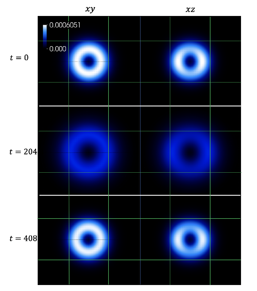
Fig. 5 displays a series of snapshots of projections in the planes and of the energy density for the run (With a large amplitude in the perturbation in the mode ) . The initial perturbation is introduced in the mode , decreasing the mass of the star and inducing a small deformation. Notice that we have taken the largest perturbation presented in this section (model ), so that the deformation can be appreciated in these projections of the energy density. At later times the system evolves and settles down into a configuration without collapsing or exploding. Although the configuration looks almost spherical, the value of at late times is slightly different from zero (. We have evolved this configuration for and remains in the same state not showing any signs of instability, or returning to a -boson star.
At this point it is important to mention that perturbations in the mode do not modify the value of the total angular momentum, while perturbations in the modes or do. Specifically, and ( and ) have a positive (negative), non-trivial and constant value of total angular momentum. As we could expect, runs like have zero angular momentum. This particular result was also obtained for the perturbations of the models that will be presented below.
IV.3.2 Non-spherical perturbation of and
The results of the previous section indicate that those configurations () that are stable under spherical perturbations do not show non-spherical growing modes. Furthermore, perturbations to the fields and applied to those configurations provide evidence for zero modes, producing new equilibrium configurations that are dynamically stable, and have small departures from the spherical configurations.
Now we are interested in studying non-spherical perturbations on configurations that might undergo gravitational collapse to a black hole. Those configurations are and . In particular , as we have mentioned, corresponds to the critical configuration with maximum ADM mass. Configuration , as is shown in Section IV.1 and reported in the literature Alcubierre:2019qnh, divides stable from unstable configurations. The latter are those configurations that can collapse into a black hole. We now go one step further and study them under non-spherical perturbations.
| Model () | Collapse | |||
|---|---|---|---|---|
| Run | ||||
| 0 | Yes | |||
| 0 | No | |||
| 0 | 0 | Yes | ||
| 0 | No | |||
| 0 | +0.01 | Yes | ||
| 0 | 0 | No | ||
| +0.01 | Yes | |||
| Yes | ||||
| Yes | ||||
| No | ||||
The list of perturbation applied to each field of is summarised in Table 4 and the result of the evolution is reported in the fifth column of the same Table. The results confirm that is the configuration that separates stable from unstable configurations. Indeed, as it can be observe in the results of Table 4, all those configurations which have perturbations that increased the total mass of the configuration undergo a collapse, while those configurations which have been perturbed and reduced the total mass of the configuration did not collapse to a black hole. In this respect, run is of special interest. The perturbation did not change the total mass of the configuration, and the result of their evolution is that it did not collapse.
Finally, we have considered non-spherical perturbations of model . The results of the evolution of the different models studied are summarised in Table 5. This configuration is on the so called unstable branch. The results mimic, to some extent, those observed for . Perturbations that reduced the total mass of the configuration led to a migration to the stable branch. On the other hand, those that increased the mass of the configuration let to a collapse into a black hole. But a key difference is seen for . This perturbation did not change the total mass of the configuration, and contrary to , it did collapse to a black hole. This result, combined with the spherical perturbations mentioned in IV.1, further confirms the special status of the maximum mass configuration : it marks the threshold of unstable configurations of -boson stars, for both spherical and non-spherical perturbations.
| Model () | Collapse | |||
|---|---|---|---|---|
| Run | ||||
| 0 | Yes | |||
| 0 | No | |||
| 0 | 0 | Yes | ||
| 0 | No | |||
| 0 | Yes | |||
| 0 | 0 | No | ||
| Yes | ||||
| Yes | ||||
| Yes | ||||
| Yes | ||||
V Discussion and Outlook
In this paper we performed dynamical simulations in the fully non-linear EKG model to investigate the stability of -boson stars. Unlike previous works we have considered non-spherical perturbations. An expected result is that those configurations known to be unstable under spherical perturbations, are also unstable under more general perturbations. The most interesting question, however, was if the configurations known to be stable under spherical perturbations would remain stable under more general ones. Here, our conclusions are two-fold. Firstly, no growing modes have been measured in our simulations. In this sense -boson stars are stable against non-spherical perturbations. However, when deformed away from sphericity, -boson stars do not return to a spherical state. They appear to oscillate around a new (slightly) non spherical state. We take this as evidence that new, multi-field, equilibrium configurations of the Einstein--Klein Gordon system exist, which are non-spherical. This conjecture is our second conclusion.
If our conjecture is proven correct, the spherically symmetric -boson stars are only an enhanced isometry point of a larger family of solutions of the Einstein--Klein Gordon. As discussed in the introduction, this is analogous to the Schwarzschild BH being the isometry enhancement point of the Kerr family. It is well known that the Kerr solution brings about qualitatively novel features with respect to the Schwarzschild solution. So it will be quite interesting to understand the novelties brought by the enlarged family of solutions that this work is suggesting.
The conjecture on the existence of these new non-spherical, multi-field configurations can be tested by solving the Einstein--Klein Gordon system for static or stationary (i.e. spinning) configurations, without assuming spherical symmetry. Research in this direction is already ongoing.
Acknowledgements.
We thank Miguel Alcubierre, Alberto Diez, Miguel Meguevand, Eugen Radu and Olivier Sarbach, for stimulating discussions. This work was supported in part by the CONACYT Network Project 280908 “Agujeros Negros y Ondas Gravitatorias”, by DGAPA-UNAM through grants IN110218, IA103616, IN105920, by the European Union’s Horizon 2020 research and innovation (RISE) program H2020-MSCA-RISE-2017 Grant No. FunFiCO-777740, by the Center for Research and Development in Mathematics and Applications (CIDMA) through the Portuguese Foundation for Science and Technology (FCT - Fundacao para a Ciência e a Tecnologia), references UIDB/04106/2020 and UIDP/04106/2020, and by the projects PTDC/FIS-OUT/28407/2017, CERN/FIS-PAR/0027/2019 and UID/FIS/00099/2020 (CENTRA). The authors would like to acknowledge networking support by the COST Action CA16104. VJ acknowledge support from CONACYT.Appendix A Code validation
For run we report the time evolution of the mass and violations of the Hamiltonian constraint, with different resolutions, , and , where , and are the sizes of the coarsest level of refinement
The L2-norm of the Hamiltonian constrain, given by , where is the number of points in the grid, is shown in Fig. 6. Here we conclude that the constraint equations converge as reduces when the resolution is increased, the black (solid) and the blue (dashed) line have been multiplied by the factors 4 and 16, showing fourth order convergence. The low resolution (solid line, coarsest grid ) corresponds to the one used in all the simulations presented in this work. The L2-norm of increases with time, however tends to a constant value which approaches zero as {.
We plot the mass for run . As the resolution is increased the mass converge to a constant value and the overall drift is reduced. In Fig. 6 and Fig. 7 we have plotted until time equal to 1300, however the () simulation extends up to , where the final total mass differs from the initial value by .


References
- [1] D. J. Kaup. Klein-gordon geon. Phys. Rev., 172:1331, 1968.
- [2] R. Ruffini and S. Bonazzola. System of self-gravitating particles in general relativity and the concept of an equation of state. Phys. Rev., 187:1767–1783, 1969.
- [3] F. E. Schunck and E. W. Mielke. General relativistic boson stars. Class. Quantum Grav., 20:R301–R356, 2003.
- [4] Steven L. Liebling and Carlos Palenzuela. Dynamical Boson Stars. Living Rev.Rel., 15:6, 2012.
- [5] T. D. Lee and Y. Pang. Stability of mini-boson stars. Nuclear Physics B, 315:477–516, March 1989.
- [6] Marcelo Gleiser. Stability of Boson Stars. Phys. Rev., D38:2376, 1988. [Erratum: Phys. Rev.D39,no.4,1257(1989)].
- [7] M. Gleiser and R. Watkins. Gravitational stability of scalar matter. Nucl. Phys., B319:733, 1989.
- [8] Fyodor V. Kusmartsev, Eckehard W. Mielke, and Franz E. Schunck. Stability of neutron and boson stars: A New approach based on catastrophe theory. 1991.
- [9] S.H. Hawley and M.W. Choptuik. Boson stars driven to the brink of black hole formation. Phys. Rev., D62:104024, 2000.
- [10] E. Seidel and W. Suen. Dynamical evolution of boson stars: Perturbing the ground state. Phys. Rev., D42:384, 1990.
- [11] F.S. Guzman. The three dynamical fates of bosons stars. Revista Mexicana de Fisica, 55(4):321–326, 2009.
- [12] Nicolas Sanchis-Gual, Carlos Herdeiro, Eugen Radu, Juan Carlos Degollado, and José A Font. Numerical evolutions of spherical proca stars. Physical Review D, 95(10):104028, 2017.
- [13] Fabrizio Di Giovanni, Nicolas Sanchis-Gual, Carlos AR Herdeiro, and José A Font. Dynamical formation of proca stars and quasistationary solitonic objects. Physical Review D, 98(6):064044, 2018.
- [14] Eckehard W. Mielke and Franz E. Schunck. Boson stars: Alternatives to primordial black holes? Nucl.Phys., B564:185–203, 2000.
- [15] D. F. Torres, S. Capozziello, and G. Lambiase. A supermassive boson star at the galactic center? Phys. Rev., D62:104012, 2000.
- [16] F. S. Guzman and J. M. Rueda-Becerril. Spherical boson stars as black hole mimickers. Phys. Rev., D80:084023, 2009.
- [17] Hector Olivares, Ziri Younsi, Christian M. Fromm, Mariafelicia De Laurentis, Oliver Porth, Yosuke Mizuno, Heino Falcke, Michael Kramer, and Luciano Rezzolla. How to tell an accreting boson star from a black hole. 2018.
- [18] C. Palenzuela, I. Olabarrieta, L. Lehner, and Steven L. Liebling. Head-on collisions of boson stars. Phys. Rev., D75:064005, 2007.
- [19] C. Palenzuela, L. Lehner, and Steven L. Liebling. Orbital Dynamics of Binary Boson Star Systems. Phys. Rev., D77:044036, 2008.
- [20] Miguel Bezares, Carlos Palenzuela, and Carles Bona. Final fate of compact boson star mergers. Physical Review D, 95(12):124005, 2017.
- [21] B. P. Abbott et al. Observation of Gravitational Waves from a Binary Black Hole Merger. Phys. Rev. Lett., 116(6):061102, 2016.
- [22] B. P. Abbott et al. GW150914: First results from the search for binary black hole coalescence with Advanced LIGO. Phys. Rev., D93(12):122003, 2016.
- [23] Tonatiuh Matos, Francisco Siddhartha Guzman, and L. Arturo Urena-Lopez. Scalar field as dark matter in the universe. Class. Quantum Grav., 17:1707–1712, 2000.
- [24] Tonatiuh Matos and L. Arturo Urena-Lopez. A further analysis of a cosmological model of quintessence and scalar dark matter. Phys. Rev., D63:063506, 2001.
- [25] Wayne Hu, Rennan Barkana, and Andrei Gruzinov. Fuzzy Cold Dark Matter: The wave properties of ultralight particles. Phys. Rev. Lett., 85:1158–1161, 2000.
- [26] Lam Hui, Jeremiah P. Ostriker, Scott Tremaine, and Edward Witten. Ultralight scalars as cosmological dark matter. Phys. Rev., D95(4):043541, 2017.
- [27] Jae-weon Lee and In-gyu Koh. Galactic halos as boson stars. Phys. Rev., D53:2236–2239, 1996.
- [28] Argelia Bernal, Juan Barranco, Daniela Alic, and Carlos Palenzuela. Multi-state Boson Stars. Phys.Rev., D81:044031, 2010.
- [29] L.Arturo Urena-Lopez and Argelia Bernal. Bosonic gas as a Galactic Dark Matter Halo. Phys.Rev., D82:123535, 2010.
- [30] Hsi-Yu Schive, Tzihong Chiueh, and Tom Broadhurst. Cosmic Structure as the Quantum Interference of a Coherent Dark Wave. Nature Phys., 10:496–499, 2014.
- [31] M. Colpi, S. L. Shapiro, and I. Wasserman. Boson stars: Gravitational equilibria of self-interacting scalar fields. Phys. Rev. Lett., 57:2485–2488, 1986.
- [32] Shijun Yoshida and Yoshiharu Eriguchi. Rotating boson stars in general relativity. Phys. Rev., D56:762–771, 1997.
- [33] France E. Schunck and Eckehard W. Mielke. Rotating boson star as an effective mass torus in general relativity. Phys. Lett. A, 249:389–394, 1998.
- [34] Richard Brito, Vitor Cardoso, Carlos AR Herdeiro, and Eugen Radu. Proca stars: gravitating bose–einstein condensates of massive spin 1 particles. Physics Letters B, 752:291–295, 2016.
- [35] Hong-Bo Li, Shuo Sun, Tong-Tong Hu, Yan Song, and Yong-Qiang Wang. Rotating multistate boson stars. Phys. Rev., D101(4):044017, 2020.
- [36] Miguel Alcubierre, Juan Barranco, Argelia Bernal, Juan Carlos Degollado, Alberto Diez-Tejedor, Miguel Megevand, Dario Nunez, and Olivier Sarbach. -Boson stars. Class. Quant. Grav., 35(19):19LT01, 2018.
- [37] Miguel Alcubierre, Juan Barranco, Argelia Bernal, Juan Carlos Degollado, Alberto Diez-Tejedor, Miguel Megevand, Darío Núñez, and Olivier Sarbach. Dynamical evolutions of -boson stars in spherical symmetry. Class. Quant. Grav., 36(21):215013, 2019.
- [38] FS Guzmán and L Arturo Ureña-López. Gravitational atoms: general framework for the construction of multistate axially symmetric solutions of the Schrödinger-Poisson system. arXiv preprint arXiv:1912.10585, 2019.
- [39] Nicolas Sanchis-Gual, Fabrizio Di Giovanni, M Zilhão, C Herdeiro, P Cerdá-Durán, JA Font, and E Radu. Nonlinear dynamics of spinning bosonic stars: Formation and stability. Physical Review Letters, 123(22):221101, 2019.
- [40] T. Regge and J. Wheeler. Stability of a Schwarzschild singularity. Phys. Rev., 108:1063–1069, 1957.
- [41] F. J. Zerilli. Effective potential for even parity Regge-Wheeler gravitational perturbation equations. Phys. Rev. Lett., 24:737, 1970.
- [42] Carlos A. R. Herdeiro and Eugen Radu. Kerr black holes with scalar hair. Phys. Rev. Lett., 112:221101, 2014.
- [43] Carlos Herdeiro, Eugen Radu, and Helgi Rúnarsson. Kerr black holes with Proca hair. Class. Quant. Grav., 33(15):154001, 2016.
- [44] Einstein Toolkit: Open software for relativistic astrophysics. http://einsteintoolkit.org/.
- [45] F Löffler. F. löffler, j. faber, e. bentivegna, t. bode, p. diener, r. haas, i. hinder, bc mundim, cd ott, e. schnetter, g. allen, m. campanelli, and p. laguna, classical quantum gravity 29, 115001 (2012). Classical Quantum Gravity, 29:115001, 2012.
- [46] Miguel Zilhão and Frank Löffler. An Introduction to the Einstein Toolkit. Int.J.Mod.Phys., A28:1340014, 2013.
- [47] Erik Schnetter, Scott H. Hawley, and Ian Hawke. Evolutions in 3D numerical relativity using fixed mesh refinement. Class. Quant. Grav., 21:1465–1488, 2004.
- [48] http://www.carpetcode.org/. Carpet: Adaptive Mesh Refinement for the Cactus Framework.
- [49] Ignacio Olabarrieta, Jason F. Ventrella, Matthew W. Choptuik, and William G. Unruh. Critical Behavior in the Gravitational Collapse of a Scalar Field with Angular Momentum in Spherical Symmetry. Phys. Rev., D76:124014, 2007.
- [50] Belen Carvente, Víctor Jaramillo, Juan Carlos Degollado, Darío Núñez, and Olivier Sarbach. Traversable -wormholes supported by ghost scalar fields. Class. Quant. Grav., 36(23):235005, 2019.
- [51] Motoyuki Saijo, Masaru Shibata, Thomas W. Baumgarte, and Stuart L. Shapiro. Dynamical bar instability in rotating stars: Effect of general relativity. Astrophys. J., 548:919–931, 2001.
- [52] Masaru Shibata and Hirotaka Yoshino. Bar-mode instability of rapidly spinning black hole in higher dimensions: Numerical simulation in general relativity. Phys. Rev., D81:104035, 2010.
- [53] Peter Diener. A new general purpose event horizon finder for 3d numerical spacetimes. Classical and Quantum Gravity, 20(22):4901, 2003.
- [54] E. Gourgoulhon. 3+1 Formalism in General Relativity, Bases of Numerical Relativity. Springer, Heidelberg, Germany, 2012.
- [55] Thomas W. Baumgarte and Stuart L. Shapiro. On the numerical integration of Einstein’s field equations. Phys. Rev., D59:024007, 1998.
- [56] David Brown, Peter Diener, Olivier Sarbach, Erik Schnetter, and Manuel Tiglio. Turduckening black holes: an analytical and computational study. Physical Review D, 79(4):044023, 2009.
- [57] Christian Reisswig, Christian D Ott, Ulrich Sperhake, and Erik Schnetter. Gravitational wave extraction in simulations of rotating stellar core collapse. Physical Review D, 83(6):064008, 2011.
- [58] M. Alcubierre. Introduction to Numerical Relativity. Oxford Univ. Press, New York, 2008.