Gauss–Markov Source Tracking with
Side Information: Lower Bounds

Motivated by recent advances in tracking and control over networks [1, 2, 3, 4, 5, 6, 7, 8, 9, 10, 11, 12, 13, 14, 15, 16, 17], we consider the setting where a decoder observes the system state corrupted by noise via an internal sensor, while it also receives quantized descriptions of the observations of the state from an external sensor over a rate-limited link.

We focus in this paper on the tracking (estimation) problem of a Gauss–Markov source over a rate-limited channel, i.e., causal encoding and decoding of the source; we view the internal noisy measurements of the state as side information that is available to the decoder but not to the encoder.

The idea of causal rate–distortion function (CRDF) was introduced in [18], where [19, 4, 20] (see also [15, 21]) drew the connection between the CRDF and tracking of a Gauss–Markov source over rate-limited links with causal encoding and decoding. Recently, two notable efforts have been made in determining bounds on the performance of these settings in the presence of decoder SI [22, 23], which provide a comprehensive set of definitions and bounds for this problem, by relying on the seminal work of Wyner and Ziv [24, 25] for rate–distortion with non-causal SI at the decoder. However, since the technique of Wyner and Ziv relies on non-causal knowledge of the SI at the decoder, applying it for scenarios with causal SI imposes an additional slack when used to bound from below the operational CRDF with (causal) SI, on top of the existing gap between the information and operational CRDFs without SI that stems from the causal encoding restriction [26, 27].

Our goal in this paper is twofold: first, providing short proofs of the lower bounds in [23] via a simple observation; secondly, deriving a tighter lower bound on the performance of causal source coding with decoder SI that is strictly higher than the bounds in [22, 23]. To derive the latter, we build on the work of Weissman and El Gamal [28] for rate–-distortion with causal SI and extend their results for CRDFs.

As a by product, we settle a conjecture in the negative by Stavrou and Skoglund [23] regarding the optimality of Wyner–Ziv-type CRDF bounds for causal tracking over additive white Gaussian noise (AWGN) channels, by proving that an adaptation of our new lower bound is strictly higher for this setting. The rest of the paper is organized as follows. In Sec. II, we formulate the problem of tracking a Gauss–Markov source over a rate-limited link for several different SI scenarios. We review classical results and tools that are used throughout this work in Sec. III. We review the CRDF scenario without SI in Sec. IV, and with two-sided SI Sec. V. We provide simple proofs for the existing results along with new tighter bounds on the CRDF with decoder SI in Sec. VI, and adopt this result to the setting of control over communication channels in Sec. VI-A.. We evaluate the expression of the new bound for a Gaussian and modulo test channels in Sec. VII.

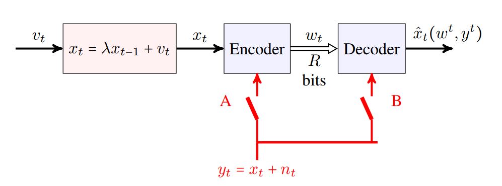
In this section, we formalize the tracking setting treated in this work, depicted in Fig. 1.

Source. The source is generated by a first order Gauss–Markov model with zero initial condition ($x_{0}=0$):¹¹ 1 The assumption $x_{0}=0$ can be easily replaced with a Gaussian $x_{0}$ that is independent of the system-disturbance sequence $\{v_{t}\}$.

where $x_{t}\in\mathbb{R}$ is the source sample at time $t$; $v_{t}$ is the system disturbance at time $t$, whose temporal entries are independent and identically distributed (i.i.d.) zero-mean Gaussian of variance $\sigma_{v}^{2}>0$; the eigenvalue $\lambda\in\mathbb{R}$ is fixed and known.

Encoder. Observes the state $x_{t}$ at time $t$ and generates a packet $a_{t}\in\left\{1,\ldots,2^{R_{t}}\right\}$ of rate $R_{t}$.

Channel. At time $t$, a packet $a_{t}\in\left\{1,2,\ldots,2^{R_{t}}\right\}$ is sent over a noiseless channel with rate $R_{t}$. The packets are subject to an average-rate constraint:²² 2 This is a more lenient constraint than the fixed-rate constraint. Consequently, our lower bounds are valid for both scenarios, although they might be too optimistic for the latter.

Side information. The SI is a noisy version of the current source sample $x_{t}$, and is given by

where $n_{t}$ is zero-mean Gaussian of variance $\sigma^{2}_{n}$, independent of $x^{t}$,³³ 3 We denote temporal sequences by $a^{t}\triangleq\left(a_{1},\ldots,a_{t}\right)$. and its temporal entries are i.i.d.

Decoder. At time $t$, receives the packet $a_{t}$ and constructs an estimate $\hat{x}_{t}$ of $x_{t}$.

Distortion. The average quadratic distortion at time $t$ is defined as

and the average-stage distortion is defined as

Different scenarios for the availability of the SI may be considered, corresponding to different states of switches A and B in Fig. 1:

• •

  No SI (A open, B open). The encoder applies a causal function $\mathcal{F}_{t}$ to the source history $x^{t}$, to generate the packet $a_{t}\in\left\{1,\ldots,2^{R_{t}}\right\}$: $a_{t}=\mathcal{F}_{t}\left(x^{t}\right)$, whereas the decoder applies a causal function $\mathcal{G}_{t}$ to the sequence of received packets $a^{t}$, to construct an estimate $\hat{x}_{t}$ of $x_{t}$: $\hat{x}_{t}=\mathcal{G}_{t}\left(a^{t}\right)$.

• •

  Two-sided SI (A closed, B closed). Here, both the encoder and the decoder have access to the SI and hence $a_{t}=\mathcal{F}_{t}\left(x^{t},y^{t}\right)$ and $\hat{x}_{t}=\mathcal{G}_{t}\left(a^{t},y^{t}\right)$.

• •

  Decoder SI (A open, B closed). Here, only the decoder has access to the SI. Thus, $a_{t}=\mathcal{F}_{t}\left(x^{t}\right)$ and $\hat{x}_{t}=\mathcal{G}_{t}\left(a^{t},y^{t}\right)$.

In this section we review known results for the scenario where SI is available to neither the encoder nor the decoder, corresponding to switches A and B being open in Fig. 1.

(16b) is derived in [18, 3, 36, 5].

For a detailed proof see [3, 5].

We now treat the two-sided SI scenario, i.e., the scenario in which the SI is available to both the encoder and the decoder, corresponding to both switches A and B being closed in Fig. 1.

The setting with two-sided SI is equivalent to the no SI setting, w.r.t. to a (Gaussian) source that is equal to $x_{t}$ given $y^{t}$. This simple observation allows a simple adaptation of the proof without SI to that of Th. 4.

In this section, we treat the more involved scenario where the SI is known only to the decoder while the encoder is oblivious of the SI, corresponding to switch A being open and B begin closed in Fig. 1.

We start by presenting a naïve lower bound.

We have seen in Lem. 2 that $R_{c}^{dec}(D)$ gives a strictly tighter lower bound than that of $R_{c}^{both}(D)$ of Lem. 1 [and that of (24)] on the operational CRDF with decoder SI. Unfortunately, carrying out the optimization in (21) and finding an explicit solution is difficult and is yet to be determined even for the simpler memoryless batch, in which it reduces to the single-letter optimization problem in (8).

Following [28], we consider a Gaussian test channel—$w_{t}=x_{t}+z_{t}$, where $z_{t}$ is a zero-mean AWGN of variance $\sigma_{z}^{2}$ in lieu of the infimum in (21) and evaluate the expression for this choice. We shall further show that Gaussian test channels are suboptimal meaning that Case 2 prevails in the proof of Lem. 2. We denote the minimum mean square errors (MMSEs) given $w^{t}$ and given $(y^{t},w^{t})$ by

First, note that $R_{1}$ equals the channel capacity of a power constrained AWGN channel [41]:

and $D_{1}=\left.\sigma_{v}^{2}\middle\|\sigma_{n}^{2}\middle\|\sigma_{z}^{2}\right.$. By substituting it in (30), we arrive at

Since rate–distortion curves must be convex and non-negative [41, Ch. 10], we clip $R_{1}$ of (31) at 0 and take its lower convex envelope to be the rate–distortion curve $R_{1}(D_{1})$.

By putting forth the the process dynamics (1) and pedestrian MMSE estimation arguments we arrive at

By defining $R_{t}(\tilde{D}_{t})\triangleq\frac{1}{2}\log\left(\lambda^{2}+\frac{\sigma_{v}^{2}}{\tilde{D}_{t}}\right)$ for $t>1$, (31), and using [5, Proof of Corol. 2], [22, Thm. 2], we have ($\tilde{D}_{0}=0$)

Using the definition of $R_{t}(\tilde{D}_{t})$ and (32), we obtain

And by equating (34) with $\tilde{D}_{t+1}$ of the definition of $R_{t+1}(\tilde{D}_{t+1})$ we attain

Substituting (35) into the recurssion of $D_{t+1}$ (32) we arrive at the recursive description:

By substituting (36) and (31) into (33) we get an expression for the average rate.

The steady-state solution for (36) is given by

where $\tilde{D}$ is the positive solution of the quadratic equation

whereas the distortion is given by the positive solution of the quadratic equation

This curve is not convex meaning that the optimal test channel in (21) is not Gaussian. Consequently, by convexifying (corresponding to time-sharing with $R=0$), we improve this curve.
We further consider one-dimensional modulo-based mappings [42, 37] and show that they outperform the TS curve of [28].

Following [43], we further consider one-dimensional modulo-based mappings [37, 42], whose equivalent test channel is given by

with $[x_{t}]_{\Delta}\triangleq x_{t}-\Delta\cdot\mathrm{round}\left(x_{t}/\Delta\right)$ and $\alpha,\beta,\Delta$ are chosen such that the power of $x_{t}$ is preserved.

We plot the resulting (convexified and 1D modulo) curves

We plot the achievable curves for $\lambda=0,0.9$, $\sigma_{n}=1/3,\sigma_{v}=1$ and compare them to $R^{\mathrm{KH}}_{c}(D)\equiv R^{\mathrm{both}}_{c}(D)$ of (17b), (24) and $R_{c}(D)$ of (16b); clearly, the TS Gaussian test-channel [28] and modulo-based [37] curves lie between the latter two. We further notice that the modulo-based mappings [37] achieve better performance than that of the TS Gaussian test-channel solution of [28].

References

- [1] E. I. Silva, M. S. Derpich, and J. Østergaard, “A framework for control system design subject to average data-rate constraints,” IEEE Trans. Auto. Cont., vol. 56, no. 8, pp. 1886–1899, Aug. 2011.
- [2] A. Sahai and S. K. Mitter, “The necessity and sufficiency of anytime capacity for stabilization of a linear system over a noisy communication link—part I: Scalar systems,” IEEE Trans. Inf. Theory, vol. 52, no. 8, pp. 3369–3395, Aug. 2006.
- [3] M. S. Derpich and J. Østergaard, “Improved upper bounds to the causal quadratic rate–distortion function for Gaussian stationary sources,” IEEE Trans. Inf. Theory, vol. 58, no. 5, pp. 3131–3152, May 2012.
- [4] S. Tatikonda, A. Sahai, and S. K. Mitter, “Stochastic linear control over a communication channel,” IEEE Trans. Auto. Cont., vol. 49, no. 9, pp. 1549–1561, Sep. 2004.
- [5] A. Khina, V. Kostina, A. Khisti, and B. Hassibi, “Tracking and control of Gauss–Markov processes over packet-drop channels with acknowledgments,” IEEE Trans. Cont. Network Sys., vol. 6, pp. 549–560, 2019.
- [6] P. A. Stavrou, J. Østergaard, C. D. Charalambous, and M. Derpich, “An upper bound to zero-delay rate distortion via Kalman filtering for vector Gaussian sources,” in Proc. IEEE Info. Theory Workshop (ITW), Kaohsiung, Taiwan, 2017, pp. 534–538.
- [7] R. Bansal and T. Başar, “Simultaneous design of measurement and control strategies for stochastic systems with feedback,” Automatica, vol. 25, no. 5, pp. 679–694, Sep. 1989.
- [8] J. S. Freudenberg, R. H. Middleton, and V. Solo, “Stabilization and disturbance attenuation over a Gaussian communication channel,” IEEE Trans. Auto. Cont., vol. 55, no. 3, pp. 795–799, Mar. 2010.
- [9] G. N. Nair and R. J. Evans, “Stabilizability of stochastic linear systems with finite feedback data rates,” SIAM J. Control and Opt., vol. 43, no. 2, pp. 413–436, 2004.
- [10] A. S. Matveev and A. V. Savkin, “An analogue of shannon information theory for detection and stabilization via noisy discrete communication channels,” SIAM journal on Control and Optimization, vol. 46, no. 4, pp. 1323–1367, Sep. 2007.
- [11] A. Khina, Y. Nakahira, Y. Su, and B. Hassibi, “Algorithms for optimal control with fixed-rate feedback,” in Proc. IEEE Conference on Decision and Control (CDC), Melbourne, VIC, Australia, Dec. 2017, pp. 6015–6020.
- [12] S. Yüksel, “Jointly optimal LQG quantization and control policies for multi-dimensional systems,” IEEE Trans. Auto. Cont., vol. 59, no. 6, pp. 1612–1617, Jun. 2014.
- [13] S. Yüksel, “Stochastic stabilization of noisy linear systems with fixed-rate limited feedback,” IEEE Trans. Auto. Cont., vol. 55, no. 12, pp. 2847–2853, Dec. 2010.
- [14] S. Yüksel and T. Başar, Stochastic Networked Control Systems: Stabilization and Optimization Under Information Constraints. Boston: Birkhäuser, 2013.
- [15] V. Kostina and B. Hassibi, “Rate–cost tradeoffs in control,” IEEE Trans. Auto. Cont., vol. 64, no. 11, pp. 4525–4540, Nov. 2019.
- [16] P. Minero, M. Franceschetti, S. Dey, and G. N. Nair, “Data rate theorem for stabilization over time-varying feedback channels,” IEEE Trans. Auto. Cont., vol. 54, no. 2, pp. 243–255, Feb. 2009.
- [17] A. Khina, E. Riedel Gårding, G. M. Pettersson, V. Kostina, and B. Hassibi, “Control over Gaussian channels with and without source–channel separation,” IEEE Trans. Auto. Cont., vol. 64, no. 9, pp. 3690–3705, Sep. 2019.
- [18] A. K. Gorbunov and M. S. Pinsker, “Prognostic epsilon entropy of a Gaussian message and a Gaussian source,” (in Russian) Problemy Pered. Info. (Problems of Info. Trans.), vol. 10, no. 2, pp. 5–25, 1974.
- [19] S. C. Tatikonda, “Control under communication constraints,” Ph.D. dissertation, Massachusetts Institute of Technology, Cambridge, CA, USA, Sep. 2000.
- [20] C. D. Charalambous, C. K. Kourtellaris, and C. Hadjicostis, “Optimal encoder and control strategies in stochastic control subject to rate constraints for channels with memory and feedback,” in Proc. IEEE Conf. Decision and Control and Euro. Control (CDC-ECC), Orlando, FL, USA, Dec. 2011, pp. 4522–4527.
- [21] T. Tanaka, P. M. Esfahani, and S. K. Mitter, “LQG control with minimum directed information: Semidefinite programming approach,” IEEE Trans. Auto. Cont., vol. 63, no. 1, pp. 37–52, Jan. 2018.
- [22] V. Kostina and B. Hassibi, “Rate-cost tradeoffs in scalar LQG control and tracking with side information,” in Proc. Allerton Conf. on Comm., Control, and Comput., Monticello, IL, USA, Oct. 2018, pp. 421–428.
- [23] P. Stavrou and M. Skoglund, “The zero-delay RDF for Gaussian processes with encoder-decoder causal side information,” Apr. 2019, qC 20190425. [Online]. Available: http://www.diva-portal.org/smash/get/diva2:1306744/FULLTEXT01.pdf
- [24] A. D. Wyner, “The Rate–Distortion function for source coding with side information at the decoder—II: General sources,” Information and Control, vol. 38, pp. 60–80, 1978.
- [25] A. D. Wyner and J. Ziv, “The Rate–Distortion function for source coding with side information at the decoder,” IEEE Trans. Inf. Theory, vol. 22, no. 1, pp. 1–10, Jan. 1976.
- [26] T. Linder and R. Zamir, “Causal coding of stationary sources and individual sequences with high resolution.” IEEE Trans. Inf. Theory, vol. 52, pp. 662–680, Feb. 2006.
- [27] D. Neuhoff and R. Gilbert, “Causal source codes,” IEEE Trans. Inf. Theory, vol. 28, no. 5, pp. 701–713, Sep. 1982.
- [28] T. Weissman and A. El Gamal, “Source coding with limited-look-ahead side information at the decoder,” IEEE Trans. Inf. Theory, vol. 52, pp. 5218–5239, Dec. 2006.
- [29] C. E. Shannon, “Coding theorems for a discrete source with a fidelity criterion,” in Institute of Radio Engineers, International Convention Record, vol. 7, 1959, pp. 142–163.
- [30] T. M. Cover and J. A. Thomas, Elements of Information Theory, Second Edition. New York: Wiley, 2006.
- [31] R. Zamir, Lattice Coding for Signals and Networks. Cambridge: Cambridge University Press, 2014.
- [32] R. Zamir, Y. Kochman, and U. Erez, “Achieving the Gaussian Rate-Distortion function by prediction,” IEEE Trans. Inf. Theory, vol. 54, pp. 3354–3364, July 2008.
- [33] Y. Kochman and R. Zamir, “Analog matching of colored sources to colored channels,” IEEE Trans. Inf. Theory, vol. 57, no. 6, pp. 3180–3195, June 2011.
- [34] J. Massey, “Causality, feedback and directed information,” in Proc. IEEE Int. Symp. Info. Theory and Its Apps. (ISITA), Waikiki, HI, USA, Nov. 1990, pp. 303–305.
- [35] G. Kramer, Directed information for channels with feedback. Lausanne, Switzerland: Hartung-Gorre, Jan. 1998.
- [36] T. Tanaka, “Semidefinite representation of sequential Rate-Distortion function for stationary Gauss–Markov processes,” in IEEE Conf. Control App. (CCA), Sydney, NSW, Australia, Sep. 2015, pp. 1217–1222.
- [37] X. Chen and E. Tuncel, “Zero-delay joint source–channel coding using hybrid digital–analog schemes in the Wyner–Ziv setting,” IEEE Trans. Comm., vol. 62, no. 2, pp. 726–735, Feb. 2014.
- [38] A. Khina and U. Erez, “Source coding with composite side information at the decoder,” in Proc. IEEE Conv. Electrical and Electron. Engineers in Israel (IEEEI), Eilat, Israel, Nov. 2012.
- [39] N. Merhav and S. Shamai, “On joint source–channel coding for the Wyner–Ziv source and the Gel’fand–Pinsker channel,” IEEE Trans. Inf. Theory, vol. 49, pp. 2844–2855, Nov. 2003.
- [40] A. El Gamal and Y.-H. Kim, Network Information Theory. Cambridge University Press, 2011.
- [41] T. M. Cover and J. A. Thomas, Elements of Information Theory. New York: Wiley, 1991.
- [42] Y. Kochman and R. Zamir, “Joint Wyner-Ziv/dirty-paper coding by modulo-lattice modulation,” IEEE Trans. Inf. Theory, vol. 55, pp. 4878–4899, Nov. 2009.
- [43] O. Lev and A. Khina, “Schemes for LQG control over Gaussian channels with side information,” arXiv preprint arXiv:2004.03927, 2020.