Bayesian semiparametric long memory models for discretized event data
Abstract
We introduce a new class of semiparametric latent variable models for long memory discretized event data. The proposed methodology is motivated by a study of bird vocalizations in the Amazon rain forest; the timings of vocalizations exhibit self-similarity and long range dependence ruling out models based on Poisson processes. The proposed class of FRActional Probit (FRAP) models is based on thresholding of a latent process consisting of an additive expansion of a smooth Gaussian process with a fractional Brownian motion. We develop a Bayesian approach to inference using Markov chain Monte Carlo, and show good performance in simulation studies. Applying the methods to the Amazon bird vocalization data, we find substantial evidence for self-similarity and non-Markovian/Poisson dynamics. To accommodate the bird vocalization data, in which there are many different species of birds exhibiting their own vocalization dynamics, a hierarchical expansion of FRAP is provided in Supplementary Materials.
Keywords: fractional Brownian motion; fractal; latent Gaussian process models; long range dependence; nonparametric Bayes; probit; time series.
1 Introduction
Event data are often obtained in a discretized form in environmental and ecological applications. Instead of recording exact times of event occurrence, one records whether or not at least one event occurred within each interval. Such data can potentially be treated as a discrete time series ((Tiao et al., 1976; Stern and Coe, 1984)) ignoring the underlying continuous time process that generated the events. While this simplification may be more amenable to standard time series analysis, it is often desirable to provide a self-explanatory stochastic model that is capable of capturing the temporal dynamics of the underlying event generating process ((Davison and Ramesh, 1996)).
In Davison and Ramesh, 1996; Ramesh et al., 2013 the authors use a Markov modulated Poisson process (MMPP) ((Fischer and Meier-Hellstern, 1993)) for the discretized events. Event intensities of an MMPP are directed by the states of an independently evolving continuous time Markov process whose different states correspond to different rates of events. Davison and Ramesh, 1996 derived expressions for the likelihood of the observed binary series for an MMPP using Chapman-Kolmogorov equations of a continuous time Markov chain. They proposed a maximum likelihood approach for inference on the model parameters, which include the instantaneous transition rate matrix of the continuous time Markov chain and the Poisson rates corresponding to each state of the chain. They also show that the autocorrelation function of the binary time series generated by an MMPP exhibits a geometric decay. Fearnhead and Sherlock, 2006 proposed a Gibbs sampling algorithm for Bayesian inference.
The geometric rate of decay in autocorrelations of an MMPP makes it inapplicable to model time series with slower decay in autocorrelations. This is true for time series where the dependence structure is non-Markovian; a special class of time series that has non-Markovian dependence and is a focus in this article is known as long range dependent series. Roughly speaking, a time series is long range dependent if its autocovariance function decays like a power function. Long range dependence has been encountered in time series data from a large variety of fields including hydrology ((Hurst, 1951)), finance ((Lo, 1989)), network traffic ((Willinger et al., 2003)), and climatology ((Franzke et al., 2020)) among others. A natural extension of the MMPP to accommodate long range dependence is the fractional Poisson process ((Laskin, 2003)). However, likelihood computation of discretized data obtained from a fractional Poisson process is not straightforward.
In seminal work, Mandelbrot and Van Ness, 1968 introduced fractional Brownian motion, a generalization of standard Brownian motion, and showed that the increments of this process are stationary and exhibit long range dependence. The general definition of fractional Brownian motion is a stochastic integral with respect to a standard Brownian motion where the order of integration is defined by a parameter . Mandelbrot and Van Ness, 1968 referred to as the Hurst parameter after the hydrologist Harold Hurst who discovered long range dependence in time series while studying storage capacities of dams on the Nile river. Mandelbrot and Van Ness, 1968 also established that the fractional Brownian motion is a self-similar stochastic process with no characteristic time-scale ((Graves et al., 2014)). Intuitively, self-similar processes retain statistical properties over different time scales and when their increments are stationary, they exhibit long range dependence.
For discretized events, the intensity of the latent counting process determines the correlation structure of the binary time series. If the binary series is long range dependent, then an inhomogeneous Poisson process with fixed intensity is insufficient to explain the observed data, as it implies that increments in disjoint time intervals are independent. Furthermore, ((Beran et al., 2016, Chapter 2)) showed that a doubly stochastic Poisson process with random intensity is long range dependent if and only if is long range dependent. Refer to Samorodnitsky et al., 2007; Pipiras and Taqqu, 2017 for reviews on long range dependence and self-similarity.
In this article, we propose a latent semiparametric framework to model long range dependent discretized event data via a FRActional Probit (FRAP) model. The FRAP model assumes a latent stochastic process responsible for generating the events of interest. Positive values of the process within a time interval imply one or more event occurrences within that interval. By setting the latent process as the fractional Brownian motion parameterized by the Hurst coefficient, we show the FRAP model is able to capture long range dependence of the discretized events. By varying the Hurst coefficient within , the spectrum of the model encompasses anti-persistence when , independence for and long range dependence when . Moreover, we also include a nonparametric trend component in our model to account for non-stationarity of event occurrences. The proposed framework accommodates testing of long range dependence in the data by comparing versus . We define a Bayesian approach to inference using a Gaussian process prior for the nonparametric trend. A Markov chain Monte Carlo (MCMC) sampling algorithm is proposed relying on sampling the latent process.
The rest of the article is organized as follows. In Section 2 we introduce the motivating Amazon bird vocalization data, including exploratory analyses revealing possible long range dependence. Section 3 is dedicated to the development and analysis of the FRAP model. Section 4 contains simulation experiments evaluating the proposed approach, and Section 5 analyzes the Amazon data. In the Supplementary Materials, we extend the FRAP model to allow multiple types of events through a grade-of-membership model and provide details on prior specification and posterior computation.
2 Amazon bird vocalization data
Bird songs play a major role in mate selection and thus have a pronounced impact on their population dynamics ((Slabbekoorn and Smith, 2002)). Identifying birds based on their vocalizations is a widely used method for estimating bird population sizes and following population trends over time, and automated acoustic monitoring is increasingly used in both ecological studies and in conservation ((Laiolo, 2010)). Bird songs are well known to follow a circadian pattern in that they sing most intensely early in the morning and late in the day ((Krebs and Kacelnik, 1983)).
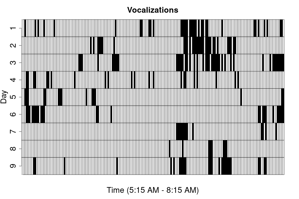
We are motivated by an Amazon bird vocalization data set containing observations from the years 2010 to 2014. Audio monitoring devices were placed at different locations throughout the Amazon rain forest. Using the methods of Ovaskainen et al., 2018, these recordings were converted to discretized binary time series ((de Camargo et al., 2019)) containing 0-1 indicators of which species vocalized at least once in one minute time intervals for a 180 minute period staring at sunrise. A visual depiction of the binary sequence of vocalizations for the bird species Automolus ochrolaemus is provided in Figure 1. Based on the audio recordings, it is not possible to reliably distinguish different individual birds of the same species or to infer the number of birds vocalizing. We focus on three locations which are similar in habitat and close in latitude and longitude. Our data consist of recordings for 15 relatively common bird species. For each species we have about 5 to 10 days of recordings during the months of June to September with recordings starting typically around 5:15 AM. On average, a given species vocalized in 25-30 out of the 180 intervals.
Our analysis focuses on two characteristics of the bird vocalization dynamics. First, we are interested in the distribution of duration of bird song activity and inactivity - in particular, our results indicate that the duration cannot be adequately modeled by the exponential distribution. In the context of event data, exponential inter-event times are routinely assumed for mathematical and computational simplicity. However, many naturally occurring events, such as earthquakes ((Ogata and Abe, 1991)), landscape evolution ((Weymer et al., 2018)), and human brain activity ((Tagliazucchi et al., 2013)), have been shown not to follow such patterns. We are also interested in identifying time periods when birds are more likely to sing and recovering groups of bird species that have similar singing patterns.

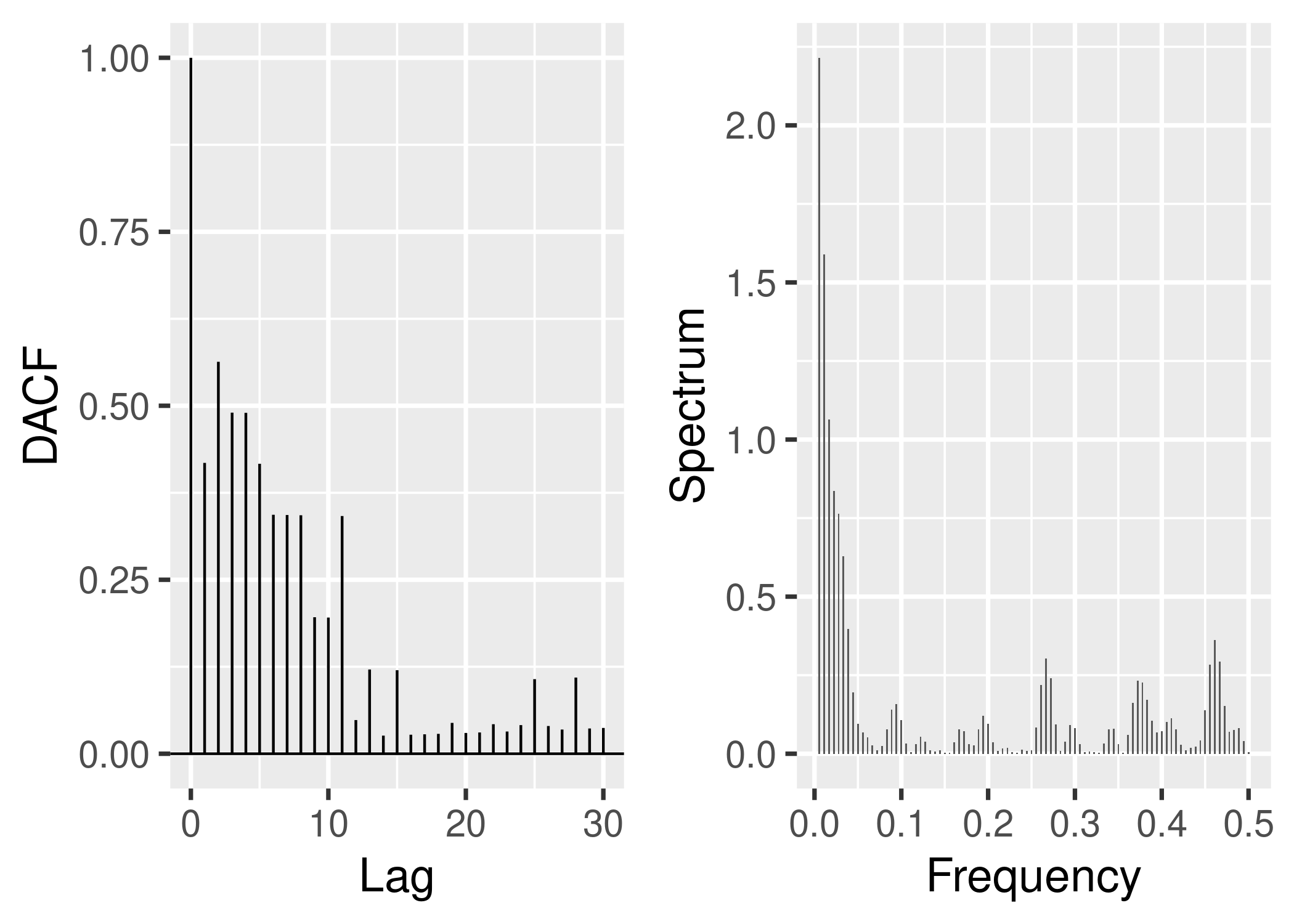
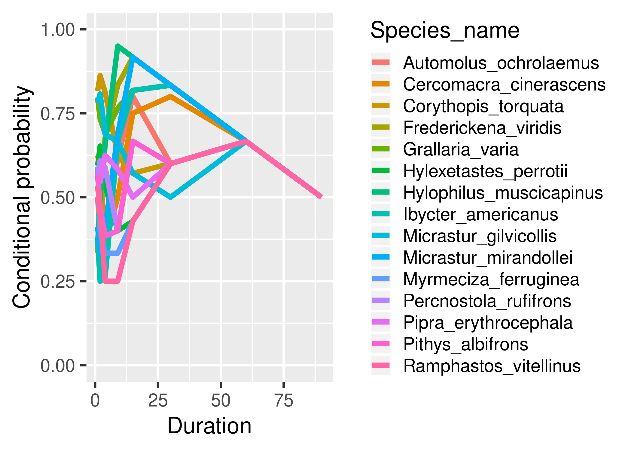
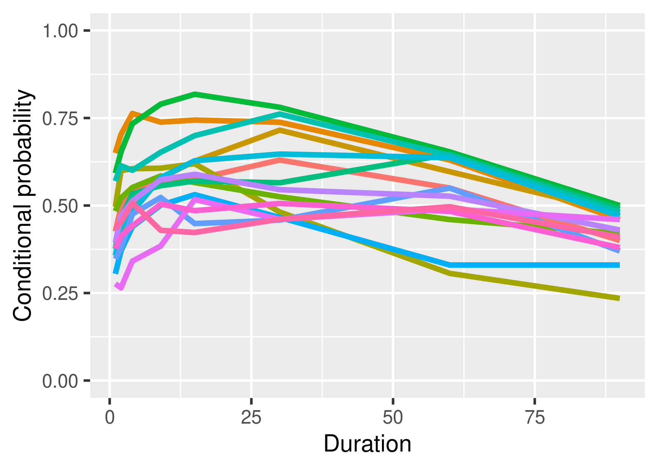
Define the marginal probability of vocalization for a given time interval of length to be the probability of observing at least one vocalization when a time interval of this length is selected at random. In the left panel of Figure 2 we show the marginal probabilities of a vocalization during minute intervals of length for 15 different bird species. On the right panel of Figure 2, we show the probabilities of vocalizations conditioned on the event that the bird vocalized in the previous interval of the same length. Quite naturally the marginal probabilities show an increasing pattern with the length of intervals. However, there is very little variation in the conditional probabilities with changes in . Such scaling of summary statistics is commonly encountered in self-similar stochastic processes ((Pipiras and Taqqu, 2017)). Additionally, the distance autocorrelations ((Zhou, 2012)) and the periodogram of the binary series for one day of recording for the species Corythopis torquata is displayed in Figure 3. The distance autocorrelation is a popular alternative to the standard autocorrelation function for investigating non-linear dependence structures and thus is more suitable for the binary time series data presented here. The slow decay in the distance autocorrelation and the spikes in the spectrum for small frequencies indicate potential long range dependence in the data.
We will use the notation for the stochastic process . A stochastic process is said to be self-similar if for any we have , so that the random variables and are equivalent in distribution up to scaling factors governed by the parameter . This parameter is commonly known as the Hurst exponent. A self-similar process with stationary increments has non-summable autocovariances ((Pipiras and Taqqu, 2017)) and is known as a long range dependent (LRD) time series. In such series, the degree of long range dependence is controlled by . For continuous time series data, many methods have been proposed to estimate : the ReScaled range (RS) analysis ((Hurst, 1951; Mandelbrot and Wallis, 1969)), detrended fluctuation analysis ((Peng et al., 1994)), log periodogram regression ((Geweke and Porter-Hudak, 1983)), local Whittle approximation ((Robinson, 1995)) etc. Although these methods typically apply to continuous data, we use these estimators in our exploratory analyses.
The rescaled range statistic of a time series is the ratio of the range of cumulative deviations from the mean to the standard deviation. Estimates of the RS statistic are obtained by dividing the time series into sub-series of different lengths and computing the RS statistic for each scale ((Bassingthwaighte and Raymond, 1994)). For a self-similar stationary time series with Hurst coefficient , Mandelbrot and Wallis, 1969 showed that the RS statistic varies roughly as where refers to the time scale. Non-stationarity in the time series may lead to false detection of long-range dependence ((Kantelhardt et al., 2001)), motivating DFA, which removes the trend in a first stage before estimating . Geweke and Porter-Hudak, 1983 proposed an alternative semiparametric approach to estimate the Hurst exponent based on the log periodogram of the data. Robinson, 1995 instead estimate using the local Whittle approximation to the likelihood.
We use R packages pracma and fractal to estimate the Hurst exponent using RS analysis and DFA, respectively; fractal allows for polynomial trends. To estimate according to Geweke and Porter-Hudak, 1983 and Robinson, 1995 we use the LongMemoryTS package in R. Table 1 shows the estimates of the Hurst exponent from the RS () analysis and DFA () with a linear trend for the 15 bird species from Figure 2 along with the estimates of according to Geweke and Porter-Hudak, 1983 () and Robinson, 1995 (). The posterior mean estimate of obtained from the proposed model here is also included in Table 1 together with the lower () and upper () 95% credible intervals. For DFA, estimates of the Hurst exponent were not sensitive to the choice of the degree of the polynomial. There is a considerable discrepancy in the estimates of from the RS and DFA analyses, with the DFA analysis surprisingly suggesting anti-persistence in the data. However, it is not clear how to obtain confidence intervals for these estimates, and whether they are entirely appropriate given that RS and DFA methods were developed for continuous and not binary time series. The estimates of as seen from and in Table 1 are closer to the estimates obtained from the proposed model although they often do not satisfy the constraint .
| Species name | |||||||||
|---|---|---|---|---|---|---|---|---|---|
| 1 | Automolus ochrolaemus | 0.67 | 0.19 | 0.83 | 0.78 | 0.67 | 0.85 | 0.89 | 0.95 |
| 2 | Cercomacra cinerascens | 0.77 | 0.17 | 1.14 | 1.07 | 0.83 | 0.90 | 0.92 | 0.94 |
| 3 | Corythopis torquata | 0.70 | 0.18 | 0.98 | 0.90 | 0.72 | 0.80 | 0.84 | 0.88 |
| 4 | Frederickena viridis | 0.75 | 0.13 | 1.12 | 1.05 | 0.63 | 0.79 | 0.86 | 0.93 |
| 5 | Grallaria varia | 0.74 | 0.14 | 1.01 | 0.94 | 0.66 | 0.84 | 0.89 | 0.93 |
| 6 | Hylexetastes perrotii | 0.70 | 0.21 | 1.01 | 0.93 | 0.85 | 0.89 | 0.93 | 0.95 |
| 7 | Hylophilus muscicapinus | 0.71 | 0.15 | 1.08 | 0.94 | 0.69 | 0.80 | 0.87 | 0.93 |
| 8 | Ibycter americanus | 0.74 | 0.25 | 1.19 | 1.11 | 0.81 | 0.90 | 0.94 | 0.96 |
| 9 | Micrastur gilvicollis | 0.70 | 0.17 | 0.98 | 0.91 | 0.64 | 0.80 | 0.84 | 0.89 |
| 10 | Micrastur mirandollei | 0.72 | 0.34 | 1.00 | 0.94 | 0.61 | 0.83 | 0.88 | 0.93 |
| 11 | Myrmeciza ferruginea | 0.70 | 0.14 | 1.00 | 0.88 | 0.61 | 0.81 | 0.85 | 0.88 |
| 12 | Percnostola rufifrons | 0.70 | 0.12 | 1.06 | 0.95 | 0.63 | 0.87 | 0.92 | 0.96 |
| 13 | Pipra erythrocephala | 0.69 | 0.20 | 0.90 | 0.85 | 0.60 | 0.79 | 0.84 | 0.88 |
| 14 | Pithys albifrons | 0.70 | 0.17 | 0.96 | 0.84 | 0.63 | 0.83 | 0.87 | 0.90 |
| 15 | Ramphastos vitellinus | 0.70 | 0.16 | 1.08 | 0.97 | 0.59 | 0.77 | 0.83 | 0.89 |
Time series models for discrete valued data with LRD structure are relatively sparse. Classical approaches for count/discrete valued times series, such as the integer autoregressive moving-average ((McKenzie, 1985; McKenzie, 1986; McKenzie, 1988)) and discrete autoregressive moving-average ((Jacobs and Lewis, 1978a; Jacobs and Lewis, 1978b)), cannot account for LRD ((Davis et al., 2016, Chapter 21)). Cui and Lund, 2009 developed a model for stationary Bernoulli sequences with LRD based on renewal sequences. Livsey et al., 2018 provide a recipe for multivariate count time series with Poisson marginals and a flexible autocovariance structure that can adequately handle LRD; see also Jia et al., 2018. Estimates of the Hurst exponent obtained from the quasi-maximum likelihood method from Livsey et al., 2018 is also included in Table 1 under the column . A major difference of the proposed method from the aforementioned works is in its ability to include non-stationarity in the data.
Our goal is not simply to estimate the Hurst coefficient; we would like to define a realistic generative probability model for these data that takes into account the data collection process and can be used as a useful baseline for future ecological analyses that include spatial dependence, environmental covariates and other complications. The estimated Hurst coefficients for our proposed fractional probit model, see Section 3.1 below, are provided in Table 1. Interestingly, the Hurst coefficients are significantly above 0.5 for all fifteen bird species. This suggests long range dependence, a new finding of ecological interest, which should be considered in future analyses of animal occurrence time series and conflicts with usual Poisson process-based models.
3 Discretized event data
We begin this section by defining some notation. Suppose event recordings are discretized at time points where the time points belong to some index set . In this article we assume that for all . Corresponding to each time interval, we have the following binary event indicators
| (1) |
We consider replications of this binary time series . In our particular setting, the replications correspond to different days of recording at a fixed location and for a fixed bird species.
3.1 Fractional probit model
Consider for now a single replication of the binary series . We assume a latent continuous time process , is responsible for instigating events of interest. Let denote the covariance function of for . We want to derive a discrete time series from so that it reflects the autocovariance structure of the observed binary data. Of particular interest are time series that exhibit long range dependence motivated by the bird vocalization data. A time series is said to have long range dependence if its autocovariance function at lag decays polynomially as ,
| (2) |
where is a slowly varying function at infinity, meaning it is positive on with and for any , . The parameter is called the long-range dependence parameter and the series is said to have long memory. A popular alternative characterization of long range dependent series relies on properties in the frequency domain. If is the spectral density of the times series , then the series is long range dependent if
| (3) |
for some slowly varying function . This definition implies that spectral densities of long range dependent series have an infinite spike in a neighborhood around 0.
The concept of long memory is intricately related to self-similarity of processes. Broadly speaking, self-similar processes are obtained as normalized limits of partial sum processes of a long memory series ((Pipiras and Taqqu, 2017)). While there are several well studied self-similar processes, one of the most fundamental and perhaps the most popular is the fractional Brownian motion (fBM). A standard Brownian motion is a stationary Gaussian process with covariance function . The fBM generalizes this covariance structure to the form
| (4) |
The parameter is known as the Hurst exponent of the fBM. Henceforth, we shall write to denote an fBM with Hurst exponent . In (4), which we set to 1. For the standard Brownian motion is recovered. The self-similarity of the process stems from the fact that . Setting , we obtain a stationary discrete time series known as fractional Gaussian noise (fGN), elements of which marginally follow a standard Gaussian distribution. The autocovariance function of is
| (5) |
where for two sequences and , implies that as . Hence, for the series is LRD in the sense of equation (2) with LRD parameter . Our proposed model relies heavily on the simple observation that if we define a series , where is a fGN with Hurst exponent , then the autocovariance function of this binary series is
| (6) |
When the series is long range dependent, that is , it follows that for large lags , since for small , i.e. the series is also long range dependent with Hurst coefficient . More generally, the inheritance of the LRD property in the binary series is true for any underlying LRD Gaussian series since (6) holds for any binary series obtained by discretizing a stationary Gaussian series. We refer the reader to ((Livsey et al., 2018, Lemma 4.1)) for the general proof. In the context of discretized event data as described in (1), we then have the following latent formulation,
| (7) |
for ; see also ((Livsey et al., 2018, Equation (4.4))) for an equivalent formulation for any latent Gaussian series. The above formulation accounts for long memory in the observed binary series, with the autocorrelation decay mimicking that of an fGN. Moreover, as a consequence of the scaling property of an fBM, a scale free property of conditional probabilities consistent with Figure 2 is established in the following Lemma.
Lemma 3.1.
Let be an fBM with Hurst coefficient with . Suppose we observe at and let , . Define the binary series of indicators at time scale , so that for , the series is as in (7). Then for any , the conditional probability is independent of the time scale . In particular,
| (8) |
Proof.
See Appendix A.1. ∎
Two remarks are in order. First, for the special case , the conditional probability in equation (8) becomes , so that when the series of indicators are generated from an underlying white noise series, the conditional probability of and the marginal probability of are equal. Second, since the function is increasing, the conditional probability of increases with , covering the cases of anti-persistence , independence and LRD for . Figure 4 depicts the relationship between the Hurst coefficient and the conditional probabilities.

Additionally, the spectral density of the series can be shown to have a pole at zero frequency when , a distinctive feature of LRD series. Let and denote the spectral density of the series and , respectively, for . Then we have for ,
where we have used the Jordan inequality for ((Mitrinovic and Vasic, 1970)). Combining this with the fact that in a neighborhood of , we see also has a pole at for and hence is LRD according to definition (3).
When considering the Amazon bird vocalization data and other real data applications, a clear limitation of model (7) is the restriction of the marginal probabilities being fixed at 0.5. To be realistic, we need to allow the marginal probabilities to be arbitrary and varying smoothly according to the time of the day. Moreover, Mikosch and Stărică, 2004; Chen et al., 2010 among many others noted that purely from a modeling perspective, long memory behavior in the sample autocovariances can be sufficiently explained by non-stationarity.
With this motivation, we introduce a non-stationary component in the FRAP model by assuming that the latent process driving the events, say , admits an additive decomposition of the form while letting
| (9) |
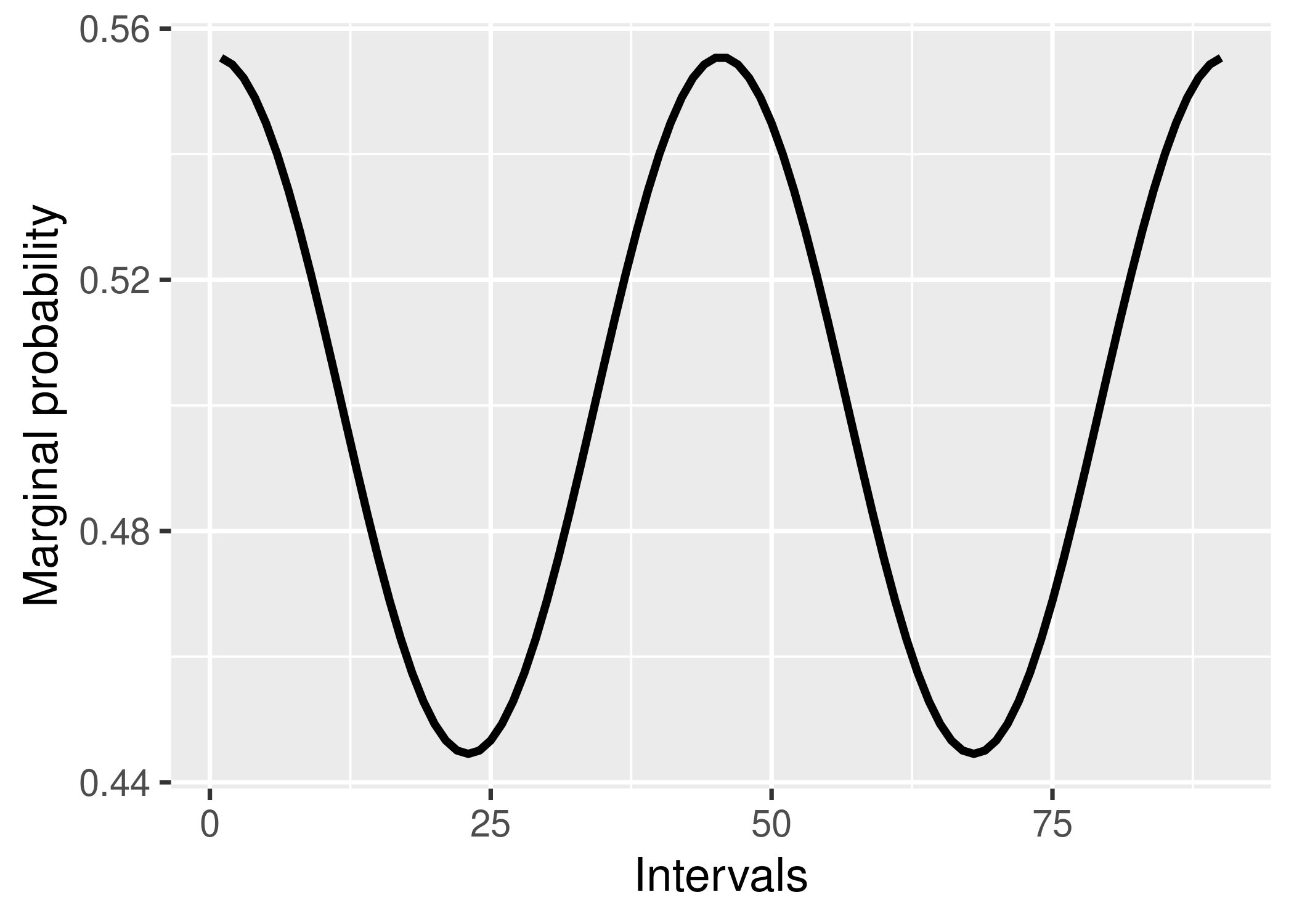
where we assume is continuously differentiable. The marginal probability of observing an event in interval is then , where is the cumulative density function of a standard Gaussian random variable. Hence, the variation in during determines the probability of observing an event during this time; a positive change increases the marginal probability, whereas a negative change decreases it. If , then the marginal probability is . To simplify notation, we write . The vector follows an -dimensional Gaussian distribution with mean and covariance matrix whose -th element is defined in equation (5). We will also include a precision parameter so that . The marginal probability of an event occurrence in the interval then becomes . In Figure 5 we show the variations in marginal probabilities when the non-stationary component in model (9) is set to with .
Akin to probit models for longitudinal binary data with covariate information ((Chib and Greenberg, 1998)) we are interested in modeling the likelihood of the observed events . However, in our context we have time series data with smooth trend and temporal dependence captured through . Letting and putting the pieces together, we get the following probit-type model,
| (10) |
where is the intersection of half-planes and the matrix is such that and for . For identifiability, we impose the restriction that . Then under model (10) is identifiable. To accommodate this restriction, we let ; the other rows of remain unchanged.
Model (10) is quite flexible in incorporating a smooth trend and auto-correlated errors. In the special case in which , the error term becomes uncorrelated so that is assumed to characterize the pattern over time in the data. When in contrast, we obtain long range dependence. The model provides a useful basis for testing of long range dependence via comparing to , in the presence of potential non-stationarity.
3.2 Priors and posterior computation
Without loss of generality, we assume that the time points . Let be the parameter space in model (10), where we let be the space of continuously differentiable functions on and . Let denote the prior on and denote the prior on . We choose and Inverse-Gamma for positive constants . For the nonparametric component, we let , where is an appropriate prior for an unknown smooth function. In particular, we choose a zero mean Gaussian process (GP) with a squared exponential covariance kernel ((Rasmussen and Williams, 2005)) scaled by the precision parameter of the latent process defined as
| (11) |
for . For numerical stability we follow the standard practice of adding a small positive quantity to the diagonal elements of the GP covariance matrix so that . Consequently, the induced prior on is again a multivariate Gaussian distribution with covariance matrix , where is an matrix with . To learn the hyperparameters from the data, we transform them to the logarithmic scale and augment the parameter space to where . We place independent standard Gaussian priors on each component of . Thus . The prior specification is completed by setting .
For the Amazon bird vocalization data, we have replications of over different days which have minimal empirical correlations. We assume these replicates are conditionally independent involving the same but with different realizations of the latent residual term leading to different realizations , for , of in equation (10). Including also the priors, this leads to the following hierarchy:
| (12) | ||||
for any and as defined after equation (10).
Posterior computation under the hierarchical FRAP model (12) is potentially challenging. We initially considered an integrated nested Laplace approximation (INLA), which was developed for approximate Bayesian inference in latent Gaussian models by Rue et al., 2009. However, the non-Markovian structure of the FRAP model renders the INLA paradigm non-applicable ((Rue and Held, 2005)). In a recent article, Sørbye and Rue, 2018 applied the INLA framework to a fGN model where the authors approximate the fGN by a mixture of first-order autoregressive processes. This approximation technique works quite well when the observed time series is quite long and the number of replications available is also very high . For the Amazon bird vocalization data both the length and the replications are quite small compare to these numbers.
- •
Update
- •
Update , where and .
- •
Update using a Metropolis random walk with proposal density .
- •
Update , where and is a matrix
with all columns equal to . - •
Update jointly via a Metropolis random walk with proposal density , where and .
We instead focus on Markov chain Monte Carlo (MCMC), developing a practical algorithm that exploits the structure of the model, as detailed in Algorithm 1. We use to denote the full conditional distribution of a parameter given other parameters and the data in Algorithm 1. The Metropolis random walk steps to update the Hurst exponent and the Gaussian process kernel hyperparameters are implemented following the adaptive Metropolis algorithm ((Roberts et al., 2001)). Adaptive Metropolis modifies the classical version of the algorithm by varying the covariance of the noise in the random walk targeting the optimal acceptance rate ((Roberts et al., 2001)). Suppose and are the noise variance of the random walk updates of and , respectively. We start with and and update them at MCMC iteration by increasing or decreasing by a factor of whenever is divisible by 50. Adaptation targets an acceptance probability of . Values of at a set of test points can also be evaluated by accommodating a further step in Algorithm 1 following ((Rasmussen and Williams, 2005, equations 2.22-2.24)).
The main computational bottleneck of Algorithm 1 involves simulating the truncated Gaussian random variables for updating the latent variables . This is done using R package tmvtnorm. Unfortunately, we found the popular circulant embedding algorithm ((Pipiras and Taqqu, 2017, Chapter 2.11)) to simulate Gaussian long range dependent sequences to be quite slow when these constraints are imposed. To accelerate computation, the copies of the latent variables are generated in parallel. The R code to implement the FRAP model given copies of discretized events is available here.
3.3 Asymptotics
Here we consider infill asymptotics so we assume we can make measurements at finer time points as within the interval . We assume the noise variance . Also, we set the number of replications since the proof does not depend on a specific value of . Let the true trend function be and the true Hurst coefficient be satisfying for some . Define and to be the true data generating probability measure and consider any weak neighborhood of . By showing that the joint prior has positive Kullback-Leibler support we have the following consistency result.
Theorem 3.2.
Suppose and for some . Write and consider any weak neighborhood of . Then the posterior probability of the set given the series of indicators in probability as .
A proof of Theorem 3.2 is provided in the Appendix.
4 Simulation experiments
We report the results of a detailed simulation study for different choices of the latent trend function in equation (9), while varying the number of replications . We assume discretized observations are available for a period of time units and the number of replications considered is . The following choices of the trend function are considered:
- 1.
- 2.
- 3.
- 4.
- 5.
.
We note here that slightly violates the assumption that the non-stationary component in model (9) at is 0. We define the squared empirical norm of a function evaluated on the points as . Given an estimator of in model (12), we evaluate the performance of Algorithm 1 by computing the Relative Mean Square Error (ReMSE) defined as , where . The latent trends are chosen from the aforementioned list and is set to be the pointwise posterior mean of at obtained under the hierarchy (12). We considered three choices for the Hurst exponent, namely, ranging from independent increments for to highly correlated increments for . We generated the binary data by first evaluating at ; to simulate the noise vector we sampled with . Representing each positive increment of by 1 the discretized series is obtained and the sampling is repeated times to complete the data generation process. For each combination of , , and we performed 30 independent evaluations of the proposed framework and in Table S.1 we report the average ReMSE and the average estimated Hurst exponent for with the value of fixed at 0.001; results for are provided in the supplementary document.
| Hurst exponent () | Replications () | MSE | MSE | MSE | MSE | MSE | |||||
|---|---|---|---|---|---|---|---|---|---|---|---|
| 0.5 | 10 | 1.26 | 0.55 | 1.02 | 0.49 | 0.12 | 0.52 | 0.09 | 0.52 | 1.38 | 0.50 |
| 25 | 0.58 | 0.48 | 0.40 | 0.48 | 0.01 | 0.50 | 0.01 | 0.51 | 0.96 | 0.51 | |
| 50 | 0.40 | 0.54 | 0.17 | 0.50 | 0.007 | 0.48 | 0.005 | 0.50 | 0.08 | 0.50 | |
| 0.75 | 10 | 2.13 | 0.76 | 1.88 | 0.76 | 0.14 | 0.74 | 0.28 | 0.76 | 4.81 | 0.74 |
| 25 | 1.37 | 0.75 | 1.20 | 0.77 | 0.06 | 0.76 | 0.03 | 0.75 | 1.46 | 0.75 | |
| 50 | 0.84 | 0.74 | 0.24 | 0.74 | 0.04 | 0.75 | 0.02 | 0.75 | 0.55 | 0.74 | |
| 0.9 | 10 | 4.18 | 0.88 | 6.52 | 0.87 | 0.70 | 0.88 | 0.20 | 0.90 | 14.96 | 0.87 |
| 25 | 3.08 | 0.89 | 2.61 | 0.89 | 0.29 | 0.89 | 0.18 | 0.89 | 5.87 | 0.93 | |
| 50 | 1.11 | 0.89 | 0.99 | 0.88 | 0.08 | 0.87 | 0.07 | 0.89 | 3.34 | 0.88 | |

Naturally, the ReMSE in Table S.1 is inversely proportional to the number of replications ; decreasing by a factor of two when the number of replications is doubled. Interestingly, the degree of LRD also controls the ReMSE. For all the choices of , the average ReMSE increases with . Large implies strong dependence in the data which makes the problem of recovering harder. This was investigated formally in Hall and Hart, 1990 who observed that the rates of recovering decrease with . Estimates of the Hurst exponent are quite accurate across all the combinations of , and . This is important in the context of the Amazon bird vocalization data for which we have on average 10 days of data. In Figure 6 we show the posterior mean and credible bands together with the true value for the marginal probabilities of events during intervals of size one time unit when the true Hurst exponent is set to and the number of replications available is . Set as the true marginal probability under model (9) with trend function and let denote samples from the posterior distribution of and obtained fitting Algorithm 1. The black line in Figure 6 is the posterior mean of the marginal probabilities and the red line plots . We also show the pointwise 95% credible bands of . The best result is obtained for . The credible bands mostly provide accurate uncertainty quantification for all the cases. However, when the number of replications is smaller the problem of accurately estimating the marginal probabilities becomes much harder, especially for high values of . Posterior samples of the Hurst exponent for one case are also included in the figure.
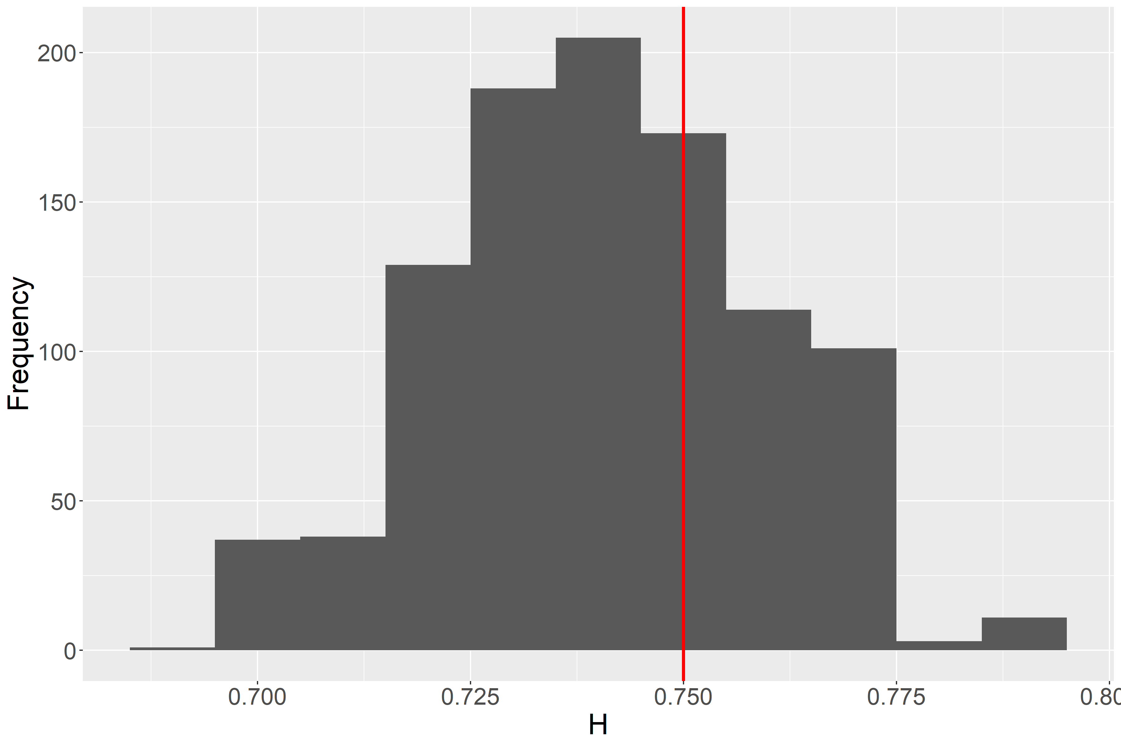
To further investigate the behavior of the posterior distribution of the Hurst exponent, we carried out an independent simulation experiment focusing on the coverage probability of the credible intervals. We fix the number of replicates at and vary the Hurst exponent together with the latent trends as above. For each such combination, we generated 100 data sets and applied model (12). Our findings for 95% credible intervals are summarized in Table 3. The coverage probabilities (CP) for all the cases considered are close to the nominal level. The average lengths (l) of the intervals vary substantially for different choices of along with the standard deviation. For example, the average length of the intervals are maximum for the case with very little variation but when the intervals become shorter on average although their variability increases by almost a factor of 3.
| CP | l | CP | l | CP | l | CP | l | CP | l | |
|---|---|---|---|---|---|---|---|---|---|---|
| 0.5 | 0.97 | 0.16(0.05) | 0.94 | 0.19(0.04) | 0.92 | 0.20(0.02) | 0.92 | 0.21(0.03) | 0.98 | 0.20(0.02) |
| 0.75 | 0.91 | 0.15(0.03) | 0.92 | 0.14(0.14) | 0.92 | 0.14(0.02) | 0.90 | 0.14(0.02) | 0.93 | 0.13(0.01) |
| 0.9 | 0.90 | 0.13(0.10) | 0.89 | 0.14(0.11) | 0.91 | 0.12(0.10) | 0.90 | 0.12(0.09) | 0.94 | 0.14(0.10) |
5 Application to Amazon bird vocalization data
5.1 Analysis and results
We applied the FRAP model to the 15 bird species mentioned in Section 2. For each of these species we have 180 minutes of recordings available for multiple days. The estimated Hurst exponents for these 15 species are reported in Table 1. All the species show high long range dependence in their temporal vocalization patterns indicating strong evidence of non-Poissonian dynamics. The posterior mean estimate of the Hurst exponent for the birds range from a minimum of 0.83 up to 0.94. The variation in the Hurst exponent across species is very small with an overall mean of 0.88 and standard deviation 0.04. The high value of the Hurst exponents is consistent with the data in the sense that birds either vocalize or remain silent over long periods of time. We note that this is a combination of two factors, which are occurrence and vocalization activity. First, due to their movement activity, a bird individual may be in the vicinity of the recorder for some time and then move to another location. Second, conditional on the bird being present, it may sustain its vocalization activity over some time and remain silent over another time.
Figure 7 shows posterior means and 95% pointwise intervals for the species-specific marginal probabilities of vocalizations occurring in each of the 180 time intervals between - AM for all 15 species listed in Table 1. Due to data sparsity and the high Hurst exponent, the raw posterior samples exhibited spiky patterns over time, and hence we (mildly) smoothed the samples prior to calculating the posterior summaries in Figure 7. While these trends should not be over-interpreted, we do see some general patterns appearing. For example, for Cercomarca cinerascens, Frederickena viridis, Grallaria varia, Micrastur mirandollei, Myrmeciza ferruginea, Percnostola ruffifrons, Pipra erythrocephala, Pithys albifrons and Ramphastos vitellinus we see an increase in vocalization activity after 7 AM, whereas Automolus ochrolaemus, Corythopis torquata, Hylexetastes perrotii, and Ibycter americanus more or less maintain a uniform activity level during this time. Micrastur gilvicollis and Hylophilus muscicapinus show more activity during the early hours of the day. Since groups of birds show similar vocalization patterns, in the Supplementary Materials Section S.1, we extend the FRAP framework to a hierarchical setting that shares information across different species.


5.2 FRAP vs MMPP
We compare the fit of the proposed FRAP model with the MMPP model ((Davison and Ramesh, 1996)) for discretized event data via summary statistics derived from the posterior distribution and maximum likelihood estimates, respectively. The particular summary statistics that we are interested are the conditional probabilities in Figure 2. In the context of the FRAP model, the distribution of the binary indicators is completely characterized by the latent variables . The posterior predictive distribution of given the observed binary indicators is , where and , . To sample the latent variable , we use the MCMC samples of obtained from Algorithm 1, i.e. given , the -th MCMC sample from , we draw . Then equation (9) is used to obtain the corresponding binary series .
The MMPP assumes event occurrence is governed by specific states of an unobserved continuous time Markov chain, hereafter referred to as CTMC, with finite state space and instantaneous transition probability matrix . Given the chain is in state at time , events occur following a Poisson process with rate . The event generating process is then parameterized by the and . The likelihood of a discretized series of events under the MMPP model has been derived in Davison and Ramesh, 1996. Let and denote the maximum likelihood estimates of and , respectively using replicates of binary event indicators . For the Amazon bird vocalization data, we generate a series of binary event indicators using the plug-in estimates and with .
Having generated event indicators from the two models for each of the 15 species in Table 1, we compute the conditional probability of occurrence of a vocalization given a vocalization in the previous interval for time scales ; for the FRAP model we compute the conditional probabilities for each MCMC sample and consider the average. In the left panel of Figure 8 we plot these probabilities using the estimates obtained from the MMPP model and in the right panel we plot the average conditional probability for different time scales across MCMC samples. The proposed FRAP model captures the scaling of the conditional probabilities seen in the observed data (Figure 2) while the MMPP does not. We also fitted the MMPP with states but the results were very similar.
5.3 Model diagnostics
We also carried out typical model diagnostics for count time series data discussed in Czado et al., 2009; Kolassa, 2016. Specifically, we use marginal calibration plots to assess model fit. We first draw samples from the predictive distribution of for a particular species of bird. We then compute using the Monte Carlo average. This predictive probability is then matched with the observed probability which is computed as . In Figure 9 we plot the differences in the predicted and observed probabilities for the 15 different species. For some birds the difference is very small whereas for other birds this difference goes up to 0.25, especially when the number of replicates available is small. Overall, the model performs adequately; prediction of vocalizations can potentially be improved by including covariates, such as weather and habitat conditions at the sampling site.

6 Discussion
In this article, we proposed a novel class of models for characterizing long range dependence in discretized event data, along with a Bayesian approach to inference under these models. We are particularly motivated by bird vocalization studies, and indeed are involved in ongoing collaborations collecting many such datasets across the globe in order to obtain new insights into biodiversity, interactions among species, and the role of biotic and abiotic factors. The proposed class of FRAP models provide an important starting point for building realistic models for these emerging datasets as well as related datasets from precipitation and storm event modeling. Immediate next directions are to add complexity to the models in order to more realistically characterize structure in the data, ranging from spatial dependence to covariate effects. Such extensions are conceptually quite straightforward.
There are several other important directions that are potentially less trivial. The first is to broaden the class of models from a latent fractional Brownian motion to a broader class of stochastic processes with long range dependence. This may include long range modifications to usual Gaussian process covariance kernels (eg, Matern), as well as non-Gaussian cases; e.g, Levy processes, alpha-stable processes, etc. The second critical direction is developing much faster computational algorithms. There is an immense literature on algorithms for accelerating computation in Gaussian process models, but to our knowledge very little consideration of the case in which there is long range dependence. In our motivating applications, we are faced with immense datasets containing automated recordings over time at many different locations around the world. To scale up to such datasets, we plan to consider divide-and-conquer algorithms and variational approximations, among other directions.
Appendix A Appendix section
A.1 Proof of Lemma 3.1
Since the fBM is a Gaussian process, from Corollary 2.6.3 of Pipiras and Taqqu, 2017 we get and for any . Hence, . By stationarity of the incremental process of fBM it is enough to show (8) holds for . Define and . Then . Also, . From (4) we get . Thus, we have . Finally, which after applying (4) again we obtain . Setting ,
A.2 Mixing of MCMC chain in Algorithm 1
We briefly comment on the mixing of the MCMC chain obtained via Algorithm 1. With MCMC samples we calculate the effective sample sizes (ESS) for the parameters and as,
| (13) |
where is the autocorrelation at lag . We set as the maximum lag and . For the 180 parameters , where , the average effective sample size for the 15 species were 2012.21 and that for the Hurst coefficient averaged over all the species is 1941.44.
A.3 Proof of Theorem 3.2
For any set the posterior probability . Now fix any weak neighborhood of . Weak consistency conditional on the latent variables is proved in Section S6 of the supplementary document. Thus the random variable converges to 0 in probability. We now extend the proof for the marginal probability . Fix any . Then we have,
where we use the fact that .
Acknowledgements
The authors acknowledge support from the United States Office of Naval Research (ONR) and the European Research Council (ERC).
Supplementary material
References
- Bassingthwaighte and Raymond, ((1994)) Bassingthwaighte, J. B. and Raymond, G. M. (1994). Evaluating rescaled range analysis for time series. Annals of Biomedical Engineering, 22(4):432–444.
- Beran et al., ((2016)) Beran, J., Feng, Y., Ghosh, S., and Kulik, R. (2016). Long-Memory Processes. Springer.
- Chen et al., ((2010)) Chen, Y., Härdle, W. K., and Pigorsch, U. (2010). Localized realized volatility modeling. Journal of the American Statistical Association, 105(492):1376–1393.
- Chib and Greenberg, ((1998)) Chib, S. and Greenberg, E. (1998). Analysis of multivariate probit models. Biometrika, 85(2):347–361.
- Chiou and Li, ((2007)) Chiou, J.-M. and Li, P.-L. (2007). Functional clustering and identifying substructures of longitudinal data. Journal of the Royal Statistical Society: Series B (Statistical Methodology), 69(4):679–699.
- Cui and Lund, ((2009)) Cui, Y. and Lund, R. (2009). A new look at time series of counts. Biometrika, 96(4):781–792.
- Czado et al., ((2009)) Czado, C., Gneiting, T., and Held, L. (2009). Predictive model assessment for count data. Biometrics, 65(4):1254–1261.
- Davis et al., ((2016)) Davis, R. A., Holan, S. H., Lund, R., and Ravishanker, N. (2016). Handbook of discrete-valued time series. CRC Press.
- Davison and Ramesh, ((1996)) Davison, A. and Ramesh, N. (1996). Some models for discretized series of events. Journal of the American Statistical Association, 91(434):601–609.
- de Camargo et al., ((2019)) de Camargo, U., Roslin, T., and Ovaskainen, O. (2019). Spatio-temporal scaling of biodiversity in acoustic tropical bird communities. Ecography, 42(11):1936–1947.
- Fearnhead and Sherlock, ((2006)) Fearnhead, P. and Sherlock, C. (2006). An exact Gibbs sampler for the Markov-modulated Poisson process. Journal of the Royal Statistical Society: Series B (Statistical Methodology), 68(5):767–784.
- Fischer and Meier-Hellstern, ((1993)) Fischer, W. and Meier-Hellstern, K. (1993). The Markov-modulated Poisson process (MMPP) cookbook. Performance evaluation, 18(2):149–171.
- Franzke et al., ((2020)) Franzke, C. L., Barbosa, S., Blender, R., Fredriksen, H.-B., Laepple, T., Lambert, F., Nilsen, T., Rypdal, K., Rypdal, M., Scotto, M. G., et al. (2020). The structure of climate variability across scales. Reviews of Geophysics, 58(2):e2019RG000657.
- Geweke and Porter-Hudak, ((1983)) Geweke, J. and Porter-Hudak, S. (1983). The estimation and application of long memory time series models. Journal of Time Series Analysis, 4(4):221–238.
- Ghosal and Van der Vaart, ((2017)) Ghosal, S. and Van der Vaart, A. (2017). Fundamentals of nonparametric Bayesian inference, volume 44. Cambridge University Press.
- Graves et al., ((2014)) Graves, T., Gramacy, R. B., Watkins, N., and Franzke, C. (2014). A brief history of long memory: Hurst, Mandelbrot and the road to ARFIMA. arXiv preprint arXiv:1406.6018.
- Hall and Hart, ((1990)) Hall, P. and Hart, J. D. (1990). Nonparametric regression with long-range dependence. Stochastic Processes and Their Applications, 36(2):339–351.
- Hurst, ((1951)) Hurst, H. E. (1951). Long-term storage capacity of reservoirs. Trans. Amer. Soc. Civil Eng., 116:770–799.
- ((19)) Jacobs, P. A. and Lewis, P. A. (1978a). Discrete time series generated by mixtures. i: Correlational and runs properties. Journal of the Royal Statistical Society: Series B (Methodological), 40(1):94–105.
- ((20)) Jacobs, P. A. and Lewis, P. A. (1978b). Discrete time series generated by mixtures ii: asymptotic properties. Journal of the Royal Statistical Society: Series B (Methodological), 40(2):222–228.
- Jacques and Preda, ((2014)) Jacques, J. and Preda, C. (2014). Model-based clustering for multivariate functional data. Computational Statistics & Data Analysis, 71:92–106.
- Jia et al., ((2018)) Jia, Y., Kechagias, S., Livsey, J., Lund, R., and Pipiras, V. (2018). Latent gaussian count time series modeling. arXiv preprint arXiv:1811.00203.
- Kantelhardt et al., ((2001)) Kantelhardt, J. W., Koscielny-Bunde, E., Rego, H. H., Havlin, S., and Bunde, A. (2001). Detecting long-range correlations with detrended fluctuation analysis. Physica A: Statistical Mechanics and its Applications, 295(3-4):441–454.
- Kolassa, ((2016)) Kolassa, S. (2016). Evaluating predictive count data distributions in retail sales forecasting. International Journal of Forecasting, 32(3):788–803.
- Krebs and Kacelnik, ((1983)) Krebs, J. R. and Kacelnik, A. (1983). The dawn chorus in the great tit (parus major): proximate and ultimate causes. Behaviour, 83(3-4):287–308.
- Laiolo, ((2010)) Laiolo, P. (2010). The emerging significance of Bioacoustics in animal species conservation. Biological conservation, 143(7):1635–1645.
- Laskin, ((2003)) Laskin, N. (2003). Fractional poisson process. Communications in Nonlinear Science and Numerical Simulation, 8(3-4):201–213.
- Livsey et al., ((2018)) Livsey, J., Lund, R., Kechagias, S., Pipiras, V., et al. (2018). Multivariate integer-valued time series with flexible autocovariances and their application to major hurricane counts. The Annals of Applied Statistics, 12(1):408–431.
- Lo, ((1989)) Lo, A. W. (1989). Long-term memory in stock market prices. Technical report, National Bureau of Economic Research.
- Mandelbrot and Van Ness, ((1968)) Mandelbrot, B. B. and Van Ness, J. W. (1968). Fractional Brownian motions, fractional noises and applications. SIAM review, 10(4):422–437.
- Mandelbrot and Wallis, ((1969)) Mandelbrot, B. B. and Wallis, J. R. (1969). Some long-run properties of geophysical records. Water resources research, 5(2):321–340.
- Manrique-Vallier, ((2010)) Manrique-Vallier, D. (2010). Longitudinal mixed membership models with applications to disability survey data. unpublished Ph. D. thesis, Department of Statistics, Carnegie Mellon University, 180.
- McKenzie, ((1985)) McKenzie, E. (1985). Some simple models for discrete variate time series 1. Journal of the American Water Resources Association, 21(4):645–650.
- McKenzie, ((1986)) McKenzie, E. (1986). Autoregressive moving-average processes with negative-binomial and geometric marginal distributions. Advances in Applied Probability, pages 679–705.
- McKenzie, ((1988)) McKenzie, E. (1988). Some arma models for dependent sequences of poisson counts. Advances in Applied Probability, pages 822–835.
- Mikosch and Stărică, ((2004)) Mikosch, T. and Stărică, C. (2004). Nonstationarities in financial time series, the long-range dependence, and the IGARCH effects. Review of Economics and Statistics, 86(1):378–390.
- Mitrinovic and Vasic, ((1970)) Mitrinovic, D. S. and Vasic, P. M. (1970). Analytic inequalities, volume 1. Springer.
- Ogata and Abe, ((1991)) Ogata, Y. and Abe, K. (1991). Some statistical features of the long-term variation of the global and regional seismic activity. International Statistical Review/Revue Internationale de Statistique, pages 139–161.
- Ovaskainen et al., ((2018)) Ovaskainen, O., Moliterno de Camargo, U., and Somervuo, P. (2018). Animal sound identifier (asi): software for automated identification of vocal animals. Ecology letters, 21(8):1244–1254.
- Pakman and Paninski, ((2014)) Pakman, A. and Paninski, L. (2014). Exact Hamiltonian Monte Carlo for truncated multivariate Gaussians. Journal of Computational and Graphical Statistics, 23(2):518–542.
- Pati et al., ((2014)) Pati, D., Bhattacharya, A., Pillai, N. S., Dunson, D., et al. (2014). Posterior contraction in sparse Bayesian factor models for massive covariance matrices. The Annals of Statistics, 42(3):1102–1130.
- Peng et al., ((1994)) Peng, C.-K., Buldyrev, S. V., Havlin, S., Simons, M., Stanley, H. E., and Goldberger, A. L. (1994). Mosaic organization of DNA nucleotides. Physical review e, 49(2):1685.
- Pipiras and Taqqu, ((2017)) Pipiras, V. and Taqqu, M. S. (2017). Long-range dependence and self-similarity, volume 45. Cambridge university press.
- Ramesh et al., ((2013)) Ramesh, N., Thayakaran, R., and Onof, C. (2013). Multi-site doubly stochastic poisson process models for fine-scale rainfall. Stochastic environmental research and risk assessment, 27(6):1383–1396.
- Rasmussen and Williams, ((2005)) Rasmussen, C. E. and Williams, C. K. I. (2005). Gaussian Processes for Machine Learning (Adaptive Computation and Machine Learning). The MIT Press.
- Roberts et al., ((2001)) Roberts, G. O., Rosenthal, J. S., et al. (2001). Optimal scaling for various Metropolis-Hastings algorithms. Statistical science, 16(4):351–367.
- Robinson, ((1995)) Robinson, P. M. (1995). Gaussian semiparametric estimation of long range dependence. The Annals of statistics, 23(5):1630–1661.
- Rodríguez et al., ((2009)) Rodríguez, A., Dunson, D. B., and Gelfand, A. E. (2009). Bayesian nonparametric functional data analysis through density estimation. Biometrika, 96(1):149–162.
- Rue and Held, ((2005)) Rue, H. and Held, L. (2005). Gaussian Markov random fields: theory and applications. Chapman and Hall/CRC.
- Rue et al., ((2009)) Rue, H., Martino, S., and Chopin, N. (2009). Approximate Bayesian inference for latent Gaussian models by using integrated nested laplace approximations. Journal of the royal statistical society: Series B (Statistical Methodology), 71(2):319–392.
- Samorodnitsky et al., ((2007)) Samorodnitsky, G. et al. (2007). Long range dependence. Foundations and Trends in Stochastic Systems, 1(3):163–257.
- Seeger et al., ((2004)) Seeger, M., Teh, Y. W., and Jordan, M. I. (2004). Semiparametric latent factor models. Technical report, Workshop on Artificial Intelligence and Statistics 10.
- Slabbekoorn and Smith, ((2002)) Slabbekoorn, H. and Smith, T. B. (2002). Bird song, ecology and speciation. Philosophical Transactions of the Royal Society of London. Series B: Biological Sciences, 357(1420):493–503.
- Sørbye and Rue, ((2018)) Sørbye, S. H. and Rue, H. (2018). Fractional Gaussian noise: Prior specification and model comparison. Environmetrics, 29(5-6):e2457.
- Spiegelhalter et al., ((2002)) Spiegelhalter, D. J., Best, N. G., Carlin, B. P., and Van Der Linde, A. (2002). Bayesian measures of model complexity and fit. Journal of the Royal Statistical society: Series B (Statistical Methodology), 64(4):583–639.
- Stephens, ((2000)) Stephens, M. (2000). Dealing with label switching in mixture models. Journal of the Royal Statistical Society: Series B (Statistical Methodology), 62(4):795–809.
- Stern and Coe, ((1984)) Stern, R. and Coe, R. (1984). A model fitting analysis of daily rainfall data. Journal of the Royal Statistical Society: Series A (General), 147(1):1–18.
- Tagliazucchi et al., ((2013)) Tagliazucchi, E., von Wegner, F., Morzelewski, A., Brodbeck, V., Jahnke, K., and Laufs, H. (2013). Breakdown of long-range temporal dependence in default mode and attention networks during deep sleep. Proceedings of the National Academy of Sciences, 110(38):15419–15424.
- Tiao et al., ((1976)) Tiao, G. C., Phadke, M., and Box, G. E. (1976). Some empirical models for the Los Angeles photochemical smog data. Journal of the Air Pollution Control Association, 26(5):485–490.
- Tokdar and Ghosh, ((2007)) Tokdar, S. T. and Ghosh, J. K. (2007). Posterior consistency of logistic gaussian process priors in density estimation. Journal of statistical planning and inference, 137(1):34–42.
- Weymer et al., ((2018)) Weymer, B. A., Wernette, P., Everett, M. E., and Houser, C. (2018). Statistical modeling of the long-range dependent structure of barrier island framework geology and surface geomorphology. Earth Surface Dynamics, 6(2):431–450.
- Willinger et al., ((2003)) Willinger, W., Paxson, V., Riedi, R. H., and Taqqu, M. S. (2003). Long-range dependence and data network traffic. Theory and applications of long-range dependence, pages 373–407.
- Zhou, ((2012)) Zhou, Z. (2012). Measuring nonlinear dependence in time-series, a distance correlation approach. Journal of Time Series Analysis, 33(3):438–457.
Supplementary materials
Bayesian semiparametric long memory models for discretized event data
Appendix S.1 Hierarchical FRAP model
The FRAP model (9) in Section 3 is designed to handle one bird species at a time. In this section we will develop an integrated model for dealing with multiple bird species having different series of event indicators , with indexing the species. For ease of exposition, we let for . However, the general case of unequal number of replicates can be handled similarly. The main motivation for extending the model proposed in the main body of the paper is to share information across similar species of birds or locations; such sharing is particularly important given the sparsity of the data, with certain bird species vocalizing only a few times on average, see Section 2.
Let denote the latent non-stationarity of the -th bird species. We assume that there are types of extremal behavioral profiles representing different patterns of vocalization behavior with time of the day. Potentially, we can attempt to assign each species to one of these profiles, leading to a type of functional clustering; for related methods, refer to Chiou and Li, 2007; Jacques and Preda, 2014; Rodríguez et al., 2009 among others. However, we view clustering as overly restrictive, and instead propose a functional mixed membership model ((Manrique-Vallier, 2010)). Let the -th extremal profile by represented as . The behavioral trajectory for species is represented by a combination of these extremal profiles having weights ,
| (S.1) |
where is the dimensional probability simplex.
The vector describes the proportional membership of the -th bird in each of the different groups. For two different species and having similar vocalization profiles, we expect the respective weight vectors and to be close. The representation of in (S.1) is also similar to a semiparametric latent factor model ((Seeger et al., 2004)) where multiple functional data are represented by a linear combination of basis functions to model dependencies across different subjects; however, our model differs in constraining the factor loadings to be constrained to the probability simplex.
We assume the same additive structure of the latent process driving the bird vocalizations as in equation (9) for the -th species on the th day, that is . The incurred dependency structure between the latent process and extremal class profiles is shown in Figure S.1 when there are 3 extremal classes. The corresponding binary series for the time interval has the following representation,
| (S.2) |
where is the realization of the fGN with Hurst exponent on the -th day, and the function satisfies the decomposition (S.1). The likelihood of the observed series can then be written as
| (S.3) |
where is defined similarly as in equation (12) and for and . The precision parameter is assumed to be equal for all realizations of the latent process across the species and days. We impose the restriction that the species vocalization profiles satisfy , or equivalently for all to ensure identifiability. The matrix is defined as in Section 3.1. We assume that the Hurst coefficient is the same across the extremal classes based on the analysis in Section 5; see also Table 1.
Appendix S.2 Priors and posterior computation
We assume is fixed and use model assessment diagnostics to choose a good value of . Recall . The unknown parameters in (S.1) include , where is the space of all by matrices such that each column of the matrix is in , is the space of continuously differentiable functions on , for . We place independent Gaussian process priors on the extremal profiles with a squared exponential covariance kernel as in equation (11) with potentially different amplitude and length-scale parameters scaled by the noise variance . We add a small positive number to the diagonals of for numerical stability. Similar to Section 3.1 we augment the parameter space with , to obtain , where . We write as the prior on . The prior on is as in Section 3.1. Similarly, we use the prior for the individual covariance kernel parameters , where each is as defined in Section 3.1.
We also need a prior distribution for . Since each column of , a natural choice is a Dirichlet prior. However, this leads to non-conjugate posterior updates. To circumvent this problem, we assign independent truncated Gaussian priors for , i.e. . In Section S.5 we describe how to sample from a - dimensional Gaussian distribution supported on a -dimensional simplex. We let denote the truncated Gaussian prior on the matrix . The prior for is from Section 3.1.
The vector can be written as , where with and . Given binary time series , we have the following representation of model (S.1),
Algorithm 1 can be extended to carry out posterior analysis for the hierarchy (). Details of our algorithm are provided below.
Let denote the prior covariance matrix for under prior . Let . Then the induced covariance matrix for is . The details of the MCMC implementation are provided below in Algorithm 2.
-
[leftmargin=*]
- •
Update , for and .
- •
Define , where and where is the matrix without the -th column and is the matrix without the -th row. Set and . Then is updated using , where and .
- •
Define and . Update where and , being the -th column of the matrix from the first step.
- •
Update using Metropolis-Hastings with proposal density .
- •
For any , is updated jointly via random walk Metropolis-Hastings.
- •
Define where and is a matrix with all columns equal to . Update .
The computational bottleneck of Algorithm 2 is in updating latent variables . In addition, the algorithm is potentially subject to label switching; this is only a problem if there is interest in the membership matrix and the corresponding extremal profiles. As in other contexts in which label switching occurs, post-processing methods can be applied to relabel the MCMC output before inferences; see, for example Stephens, 2000. In our experiments we did not encounter label switching and hence did not implement such approaches.
The Metropolis-Hastings update for in Algorithm 2 is similar to Algorithm 1 and we consider individual proposal variances for each class , which are adapted on the fly to maintain an overall acceptance probability of 0.3. Algorithm 2 performed similarly in terms of mixing assessed by the effective sample size; see Appendix of the main document. When applied to the Amazon bird vocalization data, with 10000 MCMC samples and a maximum lag of 30, the effective sample size for is 1582.61. For the elements of the membership matrix , 1240.91 is the average effective sample size and that of is 962.83.
To select the number of extremal classes, we use the Deviance Information Criterion (DIC) of Spiegelhalter et al., 2002 adapted to our latent variable setting. Let where . Then we define the DIC as,
| (S.5) |
where is the posterior mean of . We fit model () with different choices of and choose the value for which the DIC is minimized.
Appendix S.3 Simulation experiments for the hierarchical FRAP model
We considered two cases of simulation experiments implementing model (S.1). For both cases, we consider species, time units and replications. We set for these two scenarios. The species are first assigned random labels . Given species is assigned label , we set the membership vector , where , , and follows a bivariate Gaussian distribution with mean vector and covariance matrix . If the assigned label is 2, then we repeat the same steps as above but generate from a bivariate Gaussian with mean vector with the same covariance matrix. Finally, if the assigned label is 3, then we generate with mean vector . The membership vectors are then combined with extremal profiles , and to compute the individual species profile . The two choices of the extremal profiles and the resulting individual profiles are listed below:
- •
Case 1: .
- •
Case 2: .
Here we use the same definitions of the functions as in Section 4. We fixed and . Having generated the individual profiles, binary series of length are then generated following the steps from Section 4 for each species .
We implemented hierarchy () with and selected the value leading to the minimal DIC; for both cases this yielded the true value of . In the first case, the ReMSEs of the posterior mean of the three estimated extremal profiles are , and , respectively, for , and . The 95% credible interval for the Hurst coefficient for this case is . For Case 2 the ReMSE values are , and for , and , respectively. The 95% credible interval for the Hurst coefficient in this case is . In Figure S.2 we show the accuracy of the estimate of the weight matrix via a heat map.


Appendix S.4 Application to Amazon bird vocalization data
We applied the hierarchical FRAP model to the Amazon bird vocalization data with . The DIC values for are respectively 11365.4 and 10925.95. The 95% credible interval for the Hurst coefficient obtained for is . We show the posterior mean of the membership matrix in Figure S.3.

The predominant class among the birds appears to be Class 2 in Figure S.3 where Frederickena viridis, Grallaria varia, Micrastur mirandollei, Percnostola rufifrons, Pipra erythrocephala, Ramphastos vitellinus have maximum membership. This is evident from their spike in vocalization probabilities after the one and half hour mark from sunrise, see Figure 7; such a trend is apparent for Cercomarca cinerascens also. Hylexetastes perrotii, Hylophilus muscicapinus, Micrastur gilvicollis show a high membership weight on Class 3 due to their higher vocalization probabilities at the onset of the recording. Ibycter americanus, however, identifies with Class 1.
Appendix S.5 Sampling a dimensional multivariate Gaussian truncated on
Let where and . Suppose we want to sample restricted to the set , where is the dimensional simplex. We first reparameterize as , where is a dimensional vector of all 1’s. Then can be rewritten as , where and .
Under this reparameterization, it is straightforward to observe that , where and . Thus the problem of sampling on can be reformulated as sampling subject to the constraint , where and . This is done via the exact Hamiltonian truncated Gaussian sampler proposed in Pakman and Paninski, 2014.
Appendix S.6 Proof of weak consistency
We first prove weak consistency assuming the latent variables are observed. Extension of the result to the setting when we only observe the binary indicators, that is model (9), is provided in the Appendix of the main document.
Consider the model , where the design points are fixed and belong to a compact interval and we assume that . Without loss of generality we let . Suppose we observe the random variables where . Then the model for the observed random variables is where the matrix with all elements zero except and . Here . Suppose the error satisfies where . Given the data we want to recover the true parameters, say . Define . We additionally assume that for some constants and is in the space of continuously differentiable functions on . The maximum and minimum singular value of a matrix is written as and . Let , denote density of with respect to the Lebesgue measure under any generic and respectively. Since is bounded by assumption, so are and . For any fixed , we are interested in characterizing the set where for two densities and . For the densities , we have,
| (S.6) |
Unless otherwise specified, we shall write for the Euclidean norm of the vector . For a matrix , denotes the operator norm, that is, .
Lemma S.6.1.
Let be covariance matrices with Hurst coefficient and respectively and . If and , then
where is some absolute positive constant and . Furthermore,
Proof.
For the first claim see Lemma 1.3 in the supplementary document of Pati et al., 2014. To prove the second claim, we use the inequality to get . When , the lemma from Pati et al., 2014 also provides a lower bound of as . Since and , the result follows immediately as . ∎
The covariance matrix is parameterized by the Hurst coefficient where the -th element of is where . We now prove that when and are close, and are also close in the Frobenius sense.
Proposition S.6.2.
Consider the covariance matrices and for . Fix . If then for some .
Proof.
The function for fixed constants has bounded derivatives on . Hence, by the mean value theorem for some positive constant . When , we have, . ∎
In view of Lemma S.6.1 and Proposition S.6.2 the set for suitably chosen and . Recall the joint prior from the main document where . We then have that the prior probability . We trivially have that
because of the full support of the univariate Gaussian distribution on the real line. Combining the above fact with large support property of Gaussian process priors with squared exponential kernels on , the space of continuously differentiable functions, ((Tokdar and Ghosh, 2007, Theorem 4.2 - 4.4)) we have that,
This proves that for any weak neighborhood of , in probability, where is the induced measure by ((Ghosal and Van der Vaart, 2017)).
Appendix S.7 Simulation results and plots from main document
Here we summarize the simulation results from Section 4 of the main document for . Unlike the main document, here we report the error in estimating the marginal probability function. Recall that when the latent process is formulated as , then the marginal probability of observing an event according to the proposed FRAP model during any arbitrary interval is ; for this interval we write this quantity as . We estimate this using where is the posterior mean of . Finally, the cumulative error is computed by summing squares of errors over all intervals and then taking the average, i.e. where . These errors (MSE) averaged over 30 independent replicates together with estimates of the Hurst coefficient is given in the following table.
| Hurst exponent () | Replications () | MSE | MSE | MSE | MSE | MSE | ||||||
|---|---|---|---|---|---|---|---|---|---|---|---|---|
| 0.05 | 0.5 | 10 | 0.006 | 0.38 | 0.007 | 0.43 | 0.003 | 0.44 | 0.001 | 0.47 | 0.002 | 0.49 |
| 25 | 0.0009 | 0.41 | 0.001 | 0.49 | 0.0006 | 0.52 | 0.001 | 0.49 | 0.0008 | 0.52 | ||
| 50 | 0.0006 | 0.48 | 0.001 | 0.49 | 0.0003 | 0.51 | 0.0009 | 0.50 | 0.0007 | 0.50 | ||
| 0.75 | 10 | 0.004 | 0.79 | 0.003 | 0.72 | 0.009 | 0.78 | 0.005 | 0.76 | 0.004 | 0.74 | |
| 25 | 0.001 | 0.79 | 0.003 | 0.74 | 0.005 | 0.76 | 0.004 | 0.76 | 0.003 | 0.76 | ||
| 50 | 0.0007 | 0.75 | 0.001 | 0.76 | 0.0008 | 0.75 | 0.002 | 0.75 | 0.001 | 0.74 | ||
| 0.9 | 10 | 0.005 | 0.91 | 0.007 | 0.86 | 0.009 | 0.91 | 0.008 | 0.90 | 0.01 | 0.87 | |
| 25 | 0.0009 | 0.88 | 0.005 | 0.92 | 0.006 | 0.89 | 0.006 | 0.88 | 0.008 | 0.92 | ||
| 50 | 0.0007 | 0.89 | 0.002 | 0.89 | 0.002 | 0.88 | 0.003 | 0.89 | 0.002 | 0.88 | ||
| 0.15 | 0.5 | 10 | 0.008 | 0.41 | 0.008 | 0.44 | 0.008 | 0.55 | 0.005 | 0.48 | 0.006 | 0.48 |
| 25 | 0.006 | 0.45 | 0.008 | 0.48 | 0.006 | 0.51 | 0.003 | 0.48 | 0.004 | 0.51 | ||
| 50 | 0.001 | 0.49 | 0.003 | 0.50 | 0.004 | 0.51 | 0.0009 | 0.51 | 0.0009 | 0.48 | ||
| 0.75 | 10 | 0.008 | 0.77 | 0.007 | 0.73 | 0.011 | 0.78 | 0.007 | 0.78 | 0.009 | 0.78 | |
| 25 | 0.001 | 0.79 | 0.006 | 0.75 | 0.008 | 0.77 | 0.004 | 0.73 | 0.008 | 0.75 | ||
| 50 | 0.0007 | 0.75 | 0.003 | 0.75 | 0.006 | 0.74 | 0.003 | 0.74 | 0.004 | 0.74 | ||
| 0.9 | 10 | 0.009 | 0.92 | 0.001 | 0.86 | 0.013 | 0.92 | 0.010 | 0.91 | 0.012 | 0.89 | |
| 25 | 0.0009 | 0.88 | 0.008 | 0.90 | 0.009 | 0.88 | 0.008 | 0.87 | 0.009 | 0.91 | ||
| 50 | 0.0007 | 0.89 | 0.006 | 0.88 | 0.007 | 0.90 | 0.005 | 0.91 | 0.007 | 0.92 | ||


