Learning Strategies for Radar Clutter ClassificationThanks: Pia Addabbo is with Università degli studi Giustino Fortunato, Benevento, Italy. E-mail: p.addabbo@unifortunato.eu.Thanks: Sudan Han is with the National Innovation Institute of Defense Technology, Beijing, China E-mail: xiaoxiaosu0626@163.com.Thanks: Danilo Orlando is with the Engineering Faculty of Università degli Studi “Niccolò Cusano”, via Don Carlo Gnocchi 3, 00166 Roma, Italy. E-mail: danilo.orlando@unicusano.it.Thanks: Giuseppe Ricci is with the Dipartimento di Ingegneria dell’Innovazione, Università del Salento, Via Monteroni, 73100 Lecce, Italy. E-mail: giuseppe.ricci@unisalento.it.
Abstract
In this paper, we address the problem of classifying clutter returns into statistically homogeneous subsets. The classification procedures are devised assuming latent variables, which represent the classes to which each range bin belongs, and three different models for the structure of the clutter covariance matrix. Then, the expectation-maximization algorithm is exploited in conjunction with cyclic estimation procedures to come up with suitable estimates of the unknown parameters. Finally, the classification is performed by maximizing the posterior probability that a range bin belongs to a specific class. The performance analysis of the proposed classifiers is conducted over synthetic data as well as real recorded data and highlights that they represent a viable means to cluster clutter returns with respect to their range.
Index Terms:
Clutter, Diagonal Loading, Expectation-Maximization, Heterogeneous Environment, Interference Classification, Radar.I Introduction
In the past ten years, improvements in digital architectures and miniaturization technologies have wielded a significant impact in the evolution of radar systems which, consequently, are being equipped with more and more reliable and sophisticated functions [1, 2]. This increase in computational resources has led the radar community to devise detection/estimation algorithms capable of facing with challenging scenarios and, more importantly, of capitalizing on specific a priori knowledge about either the system or the environment or both. In this context, a few examples related to the structural information about the interference covariance matrix are provided by [3, 4, 5, 6, 7, 8, 9], where, at the design stage, it is assumed that the system illuminates the surveillance area through a symmetrically spaced linear array of sensors. This assumption lends both the interference covariance matrix and the steering vector a special structure which yields interesting processing gains at the price of an additional computational load [10, 11].
Other approaches relying on a priori information exploit the possible symmetries in the interference spectral properties [5, 12, 13]. As a matter of fact, ground clutter returns collected by a monostatic steady radar experience a symmetric power spectral density centered around zero-Doppler frequency [14, 15]. Remarkably, such property allows to double data used to estimate the clutter covariance matrix. Therefore, the above knowledge-based strategies represent an effective means to deal with situations where the amount of training data, used for the estimation of the interference covariance matrix, is limited (sample-starved condition) otherwise leading to low-quality estimates and, consequently, to a detection performance degradation. Besides the mentioned approaches, other widely used techniques to come up with suitable estimates of the interference covariance matrix consist in the regularization (or shrinkage) of the sample covariance matrix towards a given matrix [16, 17, 18].
However, in practice, it is not seldom to meet situations where the presence of inhomogeneities makes the interference properties estimation an even more difficult task due to the fact that such outliers should be censored as proposed in [19, 20, 21, 22]. In these contributions, suitable techniques to detect and suppress the outliers are devised in order to make the training set homogeneous. In fact, the homogeneity assumption for secondary data is a very common in detector design [23, 24, 25, 26, and references therein] and when it is no longer valid the performance degradation might become severe [27]. A more complete approach to the problem of generating homogeneous training sets would envisage an additional architectural layout capable of integrating and fusing information coming from potential heterogeneous sources to depict a clear picture of the clutter properties. These sources can be internal or external to the system and comprise mapping data, communication links, tracker feedback, or other inputs [28, 29, 30, 31].
Now, note that environment maps might be useful to identify clutter edges and to cluster data into homogeneous subsets, whose cardinality can be increased by exploiting a priori information about the clutter properties as described before. Thus, classifying (or, otherwise stated, clustering) clutter returns would represent a desirable feature for modern radar systems. Examples of clutter classifiers are provided by [32, 33], where the authors build up a neural network or process suitable features to distinguish between echoes from weather, birds, and aircrafts. Other classifiers are aimed at identifying the distribution for clutter data [34, 35, 36], the specific structure of the clutter covariance matrix [37], or the variability of clutter power over the range bins [38].
In this paper, we focus on the problem of partitioning training data into homogeneous subsets and we assume that only partial information about the environment is available at the radar receiver, namely that a given number of clutter boundaries is present. Then, we design a classification procedure capable of partitioning the secondary data set into subsets containing statistically homogeneous data. To this end, we jointly exploit the expectation-maximization (EM) algorithm [39] and the latent variable model [40]. The latter tool allows us to introduce hidden random variables which represent the classes, namely, uniform clutter regions, to which each range cell belongs. Thus, at the end of the procedure, the clustering is accomplished by estimating the a posteriori probability that a range bin belongs to a specific class. More importantly, we consider three different models for the covariance matrix of the disturbance and more precisely the following
- •
the disturbance of each class is characterized by its own Hermitian covariance matrix;
- •
different classes share a common structure of the covariance matrix, but they have different power values (clutter-dominated environment);
- •
noise returns consist of a thermal noise component (whose power is independent of the class) plus a clutter component; as in the previous case clutter returns share the same structure of the clutter covariance matrix, but each class is characterized by its own clutter power.
The preliminary performance analysis shows the effectiveness of the proposed methods in clustering data.
The remainder of the paper is organized as follows. The next section contains the problem formulation, whereas Section III is devoted to the design of the classification architectures. Illustrative examples and discussion about the classification performance are provided in Section IV. Finally, in Section V, we draw the conclusions and lay down possible future research lines. Derivations are confined to the Appendices.
I-A Notation
In the sequel, vectors and matrices are denoted by boldface lower-case and upper-case letters, respectively. The th entry of a matrix is indicated by . Symbols , , , and denote the determinant, trace, transpose, and conjugate transpose, respectively. As to numerical sets, is the set of natural numbers, is the set of real numbers, is the Euclidean space of -dimensional real matrices (or vectors if ), is the set of complex numbers, and is the Euclidean space of -dimensional complex matrices (or vectors if ). and stand for the identity matrix and the null vector or matrix of proper size. Given , indicates the diagonal matrix whose th diagonal element is . The acronym pdf and pmf stand for probability density function and probability mass function, respectively, whereas the conditional pdf of a random variable given another random variable is denoted by . Finally, we write if is a complex circular -dimensional normal vector with mean and positive definite covariance matrix while given a matrix , writing means that , , and the s are statistically independent.
II Problem Formulation and Preliminary Definitions
Consider a radar system equipped with space, time, or space-time channels which illuminates the operating area consisting of range bins. The signals backscattered by these range cells are suitably conditioned and sampled by the signal-processing unit to form -dimensional complex vectors denoted by . Now, let us assume that, from a statistical point of view, the observed environment is temporally stationary, whereas its statistical properties may change over the range due, for instance, to the presence of clutter boundaries [41]. Otherwise stated, we assume that the set of vectors can be partitioned into subsets of statistically homogeneous data; the th subset is denoted by
| (1) |
where , denotes its cardinality. Thus, the elements of share the same distributional parameters which are generally different from those associated to the distribution of , . Specifically, we assume that
| (2) |
where is unknown.
Summarizing, we are interested in estimating the subsets along with the associated unknown parameter , . To this end, in the next section we devise a classification procedure relying on the joint exploitation of the expectation maximization (EM) algorithm [39] and the latent variable model [40]. Moreover, besides the most general structure for the clutter covariance matrix, we consider two additional models which account for possible clutter power variations and diagonal loading due to thermal noise.
III Classification Architecture Designs
Data classification task is accomplished by introducing independent and identically distributed discrete random variables, s say, which take on values in with unknown pmf
| (3) |
and11 1 Recall that . such that when , then . Under this assumption, it naturally follows that the pdf of can be written as
| (4) |
where denotes the statistical expectation with respect to ,
| (5) |
, , a vector-valued function selecting the generally distinct entries of the matrix argument, and
| (6) |
Now, obtaining possible closed-form maximum likelihood estimates of the unknown parameters, namely and , is not an easy task (at least to the best of authors’ knowledge). For this reason, we resort to the EM-based algorithms, that provide closed-form updates for the parameter estimates at each step and reach at least a local stationary point. To this end, let us write the joint log-likelihood of as follows
| (7) |
As observed before, the EM algorithm is a recursive approach to the estimation of the parameter : its th iteration is aimed at computing starting from the estimate at the previous iteration, say, to form a nondecreasing sequence of log-likelihood values, namely
| (8) |
Obviously, an initial estimate of , say, is necessary to initialize the algorithm as well as a reasonable stopping criterion as, for instance, a maximum number of iterations, say. The EM consists of two steps referred to as the E-step and the M-step, respectively. The E-step leads to the computation of the following quantity
| (9) |
whereas the M-step requires to solve the following problem
| (10) |
Note that the maximization with respect to , , is independent of that over , , and, hence, we can proceed by separately addressing these two problems. Starting from the optimization over , observe that it can be solved by using the method of Lagrange multipliers, to take into account the constraint
| (11) |
Thus, it is not difficult to show that
| (12) |
Finally, in order to come up with the estimates of , we solve the following problem
| (13) |
where three different forms for the , , are considered, namely
- 1.
is a positive definite Hermitian matrix;
- 2.
, where represents the clutter power which might vary over the range profile when a clutter edge occurs, while is the common structure shared by the interference of the range bins;
- 3.
, where is the unknown thermal noise power and denotes the clutter contribution to the interference of the th range bin whose rank, say, is assumed for the moment known.
Then, the estimates of the unknown parameters for the above cases are provided by the following propositions.
Proposition 1.
Assume that , then an approximation to the relative maximum point of
| (14) |
has the following expression
| (15) |
Proof.
See Appendix A. ∎
Proposition 2.
Assume that and form for , then, given the function
| (16) |
where , an approximation to the relative maximum point can be achieved by means of the following cyclic procedure with respect to the iteration index , , (with a proper design parameter)
| (17) |
| (18) |
, and
| (19) |
, .
Proof.
See Appendix B. ∎
Proposition 3.
Assume that , , is known and form for , then an approximation to the relative maximum point of the function
| (20) |
can be obtained as follows
| (21) | ||||
| (22) |
where is the unitary matrix whose columns are the eigenvectors corresponding to the eigenvalues of the matrix
| (23) |
and
| (24) |
Proof.
See Appendix C. ∎
Note that the last proposition supposes that , , is known. However, it is clear that such assumption does not exhibit a practical value; however, the results provided by Proposition 3 can suitably be exploited in conjunction with an estimator of . To this end, we follow the lead of [42] and exploit the MOS rules to build up the following estimator for22 2 Notice that we are neglecting some constants that do not depend on and, hence, do not enter the decision process.
| (25) |
where is a penalty term related to the number of unknown parameters and has the following expression with
| (26) |
Once the unknown quantities have been estimated, data classification can be accomplished by exploiting the following rule
| (27) |
where
| (28) |
IV Illustrative Examples and Discussion
In this section, the performance of the three proposed classification architectures are assessed drawing upon synthetic data as well as real recorded data. Specifically, in the next section, the analysis is conducted by means of standard Monte Carlo counting techniques, while in the last section, the procedures are applied to the Phase One data.
IV-A Simulated Data
In the following, data are generated resorting to independent Monte Carlo trials and using two different models for the structure of the clutter covariance matrix. In the first case, we suppose the prevalence of the clutter contribution assuming an exponential shaped clutter PSD, whereas, in the second case, we do not neglect the thermal noise contribution and model the clutter samples as the summation of the echoes from patches at distinct angles. All the numerical examples assume , , and . Moreover, the presented analysis consists of a first qualitative part, where the classification outcomes of single Monte Carlo trial are shown, and a second quantitative part, where the root mean square classification error (RMSCE) is evaluated over 1000 independent Monte Carlo runs. The classification error is defined as the number of range bins whose class is not correctly identified.
IV-A1 Prevalence of the clutter contribution
The examples considered here are aimed at investigating the behavior of Proposition 1 and 2 when
| (29) |
where is the clutter power of the th class, and is the common clutter structure, such that with . It is important to observe that for the considered model, the classification procedure relying on Proposition 3 cannot be applied due to the fact that , .
As for the initialization of s, we choose equiprobable priors, namely, , whereas the initial value of is set by generating a random Hermitian structure as , where is a matrix whose columns are complex Gaussian random vectors with zero mean and identity covariance matrix. Finally, the clutter power levels are initialized as follows:
- 1.
for each range bin, compute
(30) - 2.
sort the above quantities in ascending order, ;
- 3.
the mean values of the subsets of the ordered powers is used to set the initial value of the clutter power levels, namely,
(31)
As preliminary step, we analyze the requirements of the proposed procedures in terms of number of EM iterations. To this end, in Figure 1, we plot the joint log-likelihood of versus the iteration number for Propositions 1 and 2. Specifically, the figure assumes , , , dB, dB, dB, and , where is the iteration number for the alternating maximization procedure in Proposition 2.


It turns out that, for the considered parameters, 5 iterations are sufficient to achieve convergence. Similar results are obtained also for other parameter setting but for brevity are not shown here. They point out that 10 iterations are generally sufficient for convergence. Therefore, in the next numerical examples, we set . As for , we have also analyzed its effect on the joint log-likelihood and the results show that is a proper choice.
Now, we evaluate the effect of the clutter power levels on the classification performance. To this end, we assume , , , and consider the following three cases for the clutter power levels: (1) [20,25,30] dB; (2) [20,30,40] dB; (3) [20,35,50] dB. Figure 2 shows a snapshot (to wit, a Monte Carlo outcome) for the three cases, where the estimated clutter classes are represented by ”x” red stems, whereas the true classes by the ”o” blue stems. The results highlight that for the considered parameters and from a qualitative point of view, the classification architecture based on Proposition 2 can achieve better performance than that based on Proposition 1.


A more quantitative analysis can be obtained by resorting to the RMSCE, whose values for the considered scenarios are reported in Table I.
| case (1) | case (2) | case (3) | |
| Proposition 1 | 19.85 | 2.87 | 0.29 |
| Proposition 2 | 3.10 | 0.06 | 0 |
These values confirm the superiority of the algorithm based on Proposition 2 with respect to that relying on Proposition 1, indicating that a priori information about the structure of the covariance matrix can lead to better classification performance. In fact, the simulated covariance matrix structure is more compliant with Proposition 2 than Proposition 1. In addition, as expected, the larger the power separation between different clutter classes, the lower the error values.
Finally, we evaluate the effect of different configurations for the s on the classification performance in terms of the RMSCE assuming dB, . The classification results are shown in Table II.
| [20,30,46] | [30,46,20] | [46,20,30] | [24,24,48] | [24,48,24] | [48,24,24] | [18,18,60] | [18,60,18] | [60,18,18] | |
| Prop. 1 | 21.14 | 2.52 | 7.25 | 18.63 | 4.67 | 8.04 | 39.18 | 8.50 | 28.33 |
| Prop. 2 | 0.13 | 0.09 | 0.09 | 0.10 | 0.09 | 0.08 | 18.99 | 0.09 | 1.04 |
The superiority of the classification architecture based on Proposition 2 is further validated. Moreover, it is worth noticing that the more challenging case for both Propositions is when the number of clutter classes with lower clutter power is much smaller than that of the clutter class with high clutter power, namely, . This behavior can be explained by the fact that the classification procedures tend to merge small classes with low powers.
IV-A2 Distributed clutter plus thermal noise
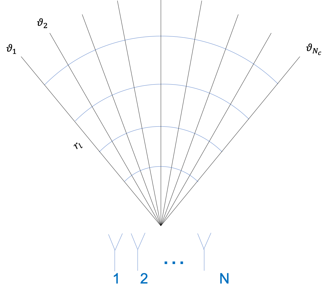
In this subsection, we assume another clutter covariance matrix model. As shown in Figure 3, we consider a uniformly-spaced linear array of identical and isotropic sensors with inter-element distance equal to , where is the wavelength corresponding to the radar carrier frequency. We only consider the spatial processing for simplicity and model the clutter samples as the summation of individual patch returns at distinct angles [43], leading to the following covariance structure
| (32) |
where
- •
(for simplicity, we suppose that the number of the angular sectors is the same for each class, namely, for all );
- •
is the spatial steering vector whose expression is given by .
In the following, we set , the beam pointing direction to , and an angular sector within the first null beamwidth of , namely, .
The initialization method is the same as that in the Subsection IV-A1. Moreover, as to Proposition 3, we consider two situations, i.e., the clutter rank is known and is unknown. In the latter case, the GIC rule with is exploited to estimate using (25).


Figure 4 shows the joint log-likelihood versus the iteration number of the EM procedure for , , , dB, dB and dB. The curves confirm that a few iterations are sufficient for convergence.


| case (1) | case (2) | case (3) | |
|---|---|---|---|
| Proposition 1 | 26.29 | 5.87 | 1.03 |
| Proposition 2 | 43.89 | 33.08 | 29.21 |
| Proposition 3, known | 29.16 | 5.64 | 0.87 |
| Proposition 3, unknown | 29.94 | 5.81 | 0.97 |
A qualitative analysis is provided by Figures 5-7, where Monte Carlo outcomes for the same clutter power configurations as in Section IV-A1 are shown (assuming ). The curves highlight that, for the considered parameters, the classification methods based on Propositions 1 and 3 share almost the same performance. As to Proposition 2, it exhibits the worst performance.
The RMSCE for different clutter power levels are shown in Table III. The obtained values confirm that the classification performances for Propositions 1 and 3 are very close to each other and are much better than that based on Proposition 2.
| [20,30,46] | [30,46,20] | [46,20,30] | [24,24,48] | [24,48,24] | [48,24,24] | [18,18,60] | [18,60,18] | [60,18,18] | |
| Prop. 1 | 20.48 | 8.32 | 10.29 | 18.37 | 8.29 | 15.70 | 37.36 | 13.12 | 38.32 |
| Prop. 2 | 37.66 | 29.19 | 24.99 | 35.84 | 27.90 | 25.97 | 44.59 | 22.11 | 35.72 |
| Prop. 3, | 19.44 | 6.74 | 7.99 | 17.23 | 7.54 | 11.76 | 35.66 | 11.24 | 37.73 |
| known | |||||||||
| Prop. 3, | 18.55 | 6.83 | 7.29 | 16.29 | 7.58 | 11.00 | 35.28 | 10.84 | 38.28 |
| unknown |
Table IV contains the RMSCE values for different configurations. Inspection of the table indicates that the classification algorithm based on Proposition 3 can guarantee better performance than that based on Proposition 1. In addition, the knowledge of does not significantly affects the resulting performance. Finally, Proposition 2 continues to return the highest error values.
IV-B Real data
In this section, we assess the performance analysis on real L-band land clutter data, recorded in 1985 using the MIT Lincoln Laboratory Phase One radar at the Katahdin Hill site, MIT Lincoln Laboratory. We consider datasets contained in the files and , which are composed of temporal returns from range cells with VV and HH-polarization, respectively. More details about this dataset can be found in [44, 45, 46] and references therein.
The 3-D clutter intensity field, from the Phase One file , is plotted in Figure 8. It is evident the presence of two regions with different power levels (region 1 from cell 1 to cell 48 and region 2 from cell 49 to cell 76). This behavior, already observed in [46], is due to the fact that data were measured from range cells containing agricultural fields in contrast to windblown vegetation. Other five major terrain categories, distributed within the two major regions, are also evident, as indicated in figure. The 3-D normalized intensity plot relative to the data file is reported in Figure 9). Here, three major areas with different power levels can be identified.
These data are fed to the proposed algorithms and the used parameters are:
- •
;
- •
;
- •
or ;
- •
a maximum number iterations of 10 (for both EM and alternating procedure).
Classification results, relative to the dataset, are reported in Figures 10 and 11, for a number of classes of three and five, respectively. Data are characterized by small temporal variations of the power (variations in time on a given range cell, or on few cells) due to the inherent characteristic of the observed scene. Thus, the estimated classes are compared with power levels averaged over 100 temporal samples near the selected temporal samples. The inspection of the figure points out that estimated classes follow the power profile for both and . For this dataset, five classes allow to distinguish between all the five terrains indicated in Figure 8.
The classification results for dataset are shown in Figures 12 and 13, respectively, and confirm what observed in the previous figures.


V Conclusions
This paper has proposed several algorithms to classify clutter radar echoes with the goal of partitioning the possibly heterogeneous training dataset into homogeneous subsets, which, then, can be used for estimation/detection purposes. The algorithms have been designed using the EM algorithm in conjunction with the latent variable model. More precisely, considering three different structures for the clutter covariance matrix (from the most general case of a Hermitian structure to the specific one where diagonal loading is accounted for) three different classification architectures have been introduced. Performance analysis for both simulated and real data has clearly shown the capability of the proposed approach to solve the problem of clutter data clustering. More importantly, these schemes can be used as preliminary stage of a detection architecture, where the detection stage exploits the information provided by the classifier to process homogeneous data.
Future research tracks include the design of clustering algorithms in the presence of outliers, which can be discarded once identified. Another issue is related to further structures for the clutter covariance matrix that can improve the estimation quality and, hence, detection performance of those receivers relying on such estimates. Finally, the design of architectures for the joint detection and classification of clutter edges represent an important extension of this work. All the above topics represent the current research activity.
Appendix A Proof of Proposition 1
Let us consider the following problem
| (33) |
which is tantamount to solving
| (34) |
for each . To this end, we set to zero the first derivative of with respect to [47], namely
| (35) |
The solution of the above equation is given by
| (36) |
and the proof is complete.
Appendix B Proof of Proposition 2
In order to come up with the estimates of the s and , we set to zero the first derivatives of (with respect to the s and ), namely
| (37) |
and
| (38) |
The equations can be re-written as
| (39) |
and
| (40) |
respectively, where we have used the fact that
| (41) |
Since the equation system formed by (39) and (40) does not admit a closed-form solution, we propose to resort to alternating maximization; based on and we first compute the s by plugging into eqs. (39); then, we compute by plugging the s into eq. (40). This procedure can be iterated obtaining, after iterations, the s and . To conclude the proof we observe that both EM and alternating maximization lead to a non decreasing sequence of likelihood values [48].
Appendix C Proof of Proposition 3
First we re-write (20) as follows
and also as
| (42) |
where . Now, let us consider the eigendecomposition of , namely
where is a unitary matrix whose columns are the eigenvectors of while is the corresponding diagonal matrix of the eigenvalues of ; can be represented as with . It follows that the objective function becomes
where
Replacing by its eigendecomposition, we also come up with
where with being the eigenvalues of and the unitary matrix of the corresponding eigenvectors. As a consequence, the objective function (42) can also be recast as
where and . Exploiting Theorem 1 of [49], it is possible to show that
which implies that . Then, we obtain
| (43) | ||||
As the next step towards the final result, we set to zero the first derivative of the above objective function with respect to , , namely
After replacing with in (43), the last optimization is
which can be solved by finding the zeros of the following function
The result is
| (46) |
Finally, the estimate of , , , is given by
| (47) |
and the proof is complete.
References
- [1] W. L. Melvin and J. A. Scheer, Principles of Modern Radar: Advanced Techniques, S. Publishing, Ed., Edison, NJ, 2013.
- [2] M. A. Richards, W. L. Melvin, J. A. Scheer, and W. A. Holm, Principles of Modern Radar: Radar Applications, Volume 3, ser. Electromagnetics and Radar. Institution of Engineering and Technology, 2013.
- [3] J. Liu, W. Liu, H. Liu, B. Chen, X. G. Xia, and F. Dai, “Average SINR Calculation of a Persymmetric Sample Matrix Inversion Beamformer,” IEEE Transactions on Signal Processing, vol. 64, no. 8, pp. 2135–2145, April 2016.
- [4] J. Liu, S. Sun, and W. Liu, “One-step persymmetric GLRT for subspace signals,” IEEE Transaction on Signal Processing, vol. 14, no. 67, pp. 3639–3648, July 15 2019.
- [5] G. Foglia, C. Hao, G. Giunta, and D. Orlando, “Knowledge-aided adaptive detection in partially homogeneous clutter: Joint exploitation of persymmetry and symmetric spectrum,” Digital Signal Processing, vol. 67, no. Supplement C, pp. 131 – 138, 2017.
- [6] L. Cai and H. Wang, “A Persymmetric Multiband GLR Algorithm,” IEEE Transactions on Aerospace and Electronic Systems, vol. 28, no. 3, pp. 806–816, 1992.
- [7] P. Wang, Z. Sahinoglu, M. Pun, and H. Li, “Persymmetric Parametric Adaptive Matched Filter for Multichannel Adaptive Signal Detection,” IEEE Transactions on Signal Processing, vol. 60, no. 6, pp. 3322–3328, 2012.
- [8] C. Hao, S. Gazor, G. Foglia, B. Liu, and C. Hou, “Persymmetric adaptive detection and range estimation of a small target,” IEEE Transactions on Aerospace and Electronic Systems, vol. 51, no. 4, pp. 2590–2604, 2015.
- [9] G. Pailloux, P. Forster, J. P. Ovarlez, and F. Pascal, “Persymmetric Adaptive Radar Detectors,” IEEE Transactions on Aerospace and Electronic Systems, vol. 47, no. 4, pp. 2376–2390, 2011.
- [10] R. Nitzberg, “Application of Maximum Likelihood Estimation of Persymmetric Covariance Matrices to Adaptive Processing,” IEEE Transactions on Aerospace and Electronic Systems, vol. 16, no. 1, pp. 124–127, 1980.
- [11] H. L. Van Trees, Optimum Array Processing (Detection, Estimation, and Modulation Theory, Part IV). John Wiley & Sons, 2002.
- [12] G. Foglia, C. Hao, A. Farina, G. Giunta, D. Orlando, and C. Hou, “Adaptive Detection of Point-Like Targets in Partially Homogeneous Clutter With Symmetric Spectrum,” IEEE Transactions on Aerospace and Electronic Systems, vol. 53, no. 4, pp. 2110–2119, 2017.
- [13] A. De Maio, D. Orlando, C. Hao, and G. Foglia, “Adaptive Detection of Point-like Targets in Spectrally Symmetric Interference,” IEEE Transactions on Signal Processing, vol. 64, no. 12, pp. 3207–3220, 2016.
- [14] J. B. Billingsley, Low-angle radar land clutter - Measurements and empirical models. Norwich, NY: William Andrew Publishing, 2002.
- [15] J. B. Billingsley, A. Farina, F. Gini, M. S. Greco, and L. Verrazzani, “Statistical Analyses of Measured Radar Ground Clutter Data,” IEEE Transactions on Aerospace and Electronic Systems, vol. 35, no. 2, pp. 579–593, 1999.
- [16] Y. Chen, A. Wiesel, and A. O. Hero, “Robust shrinkage estimation of high-dimensional covariance matrices,” IEEE Transactions on Signal Processing, vol. 59, no. 9, pp. 4097–4107, Sep. 2011.
- [17] E. Ollila and D. E. Tyler, “Regularized -Estimators of Scatter Matrix,” IEEE Transactions on Signal Processing, vol. 62, no. 22, pp. 6059–6070, Nov 2014.
- [18] M. Steiner and K. Gerlach, “Fast converging adaptive processor or a structured covariance matrix,” IEEE Transactions on Aerospace and Electronic Systems, vol. 36, no. 4, pp. 1115–1126, Oct 2000.
- [19] M. C. Wicks, W. L. Melvin, and P. Chen, “An efficient architecture for nonhomogeneity detection in space-time adaptive processing airborne early warning radar,” in Radar 97 (Conf. Publ. No. 449), Oct 1997, pp. 295–299.
- [20] R. S. Adve, T. B. Hale, and M. C. Wicks, “Transform domain localized processing using measured steering vectors and non-homogeneity detection,” in Proceedings of the 1999 IEEE Radar Conference. Radar into the Next Millennium (Cat. No.99CH36249), April 1999, pp. 285–290.
- [21] B. Himed, Y. Salama, and J. H. Michels, “Improved detection of close proximity targets using two-step nhd,” in Record of the IEEE 2000 International Radar Conference [Cat. No. 00CH37037], May 2000, pp. 781–786.
- [22] M. Rangaswamy, B. Himed, and J. H. Michels, “Performance analysis of the nonhomogeneity detector for stap applications,” in Proceedings of the 2001 IEEE Radar Conference (Cat. No.01CH37200), May 2001, pp. 193–197.
- [23] E. J. Kelly, “An adaptive detection algorithm,” IEEE Transactions on Aerospace and Electronic Systems, no. 2, pp. 115–127, 1986.
- [24] F. C. Robey, D. R. Fuhrmann, E. J. Kelly, and R. Nitzberg, “A CFAR adaptive matched filter detector,” IEEE Transactions on Aerospace and Electronic Systems, vol. 28, no. 1, pp. 208–216, 1992.
- [25] F. Bandiera, D. Orlando, and G. Ricci, Advanced Radar Detection Schemes Under Mismatched Signal Models. San Rafael, US: Synthesis Lectures on Signal Processing No. 8, Morgan & Claypool Publishers, 2009.
- [26] E. Conte, A. De Maio, and G. Ricci, “GLRT-based adaptive detection algorithms for range-spread targets,” IEEE Transactions on Signal Processing, vol. 49, no. 7, pp. 1336–1348, July 2001.
- [27] W. L. Melvin, “Space-time Adaptive Radar Performance in Heterogeneous Clutter,” IEEE Transactions on Aerospace and Electronic Systems, vol. 36, no. 2, pp. 621–633, 2000.
- [28] W. L. Melvin, M. Wicks, P. Antonik, Y. Salama, Ping Li, and H. Schuman, “Knowledge-based space-time adaptive processing for airborne early warning radar,” IEEE Aerospace and Electronic Systems Magazine, vol. 13, no. 4, pp. 37–42, 1998.
- [29] G. T. Capraro, A. Farina, H. Griffiths, and M. C. Wicks, “Knowledge-based radar signal and data processing: a tutorial review,” IEEE Signal Processing Magazine, vol. 23, no. 1, pp. 18–29, 2006.
- [30] M. C. Wicks, M. Rangaswamy, R. Adve, and T. B. Hale, “Space-time adaptive processing: a knowledge-based perspective for airborne radar,” IEEE Signal Processing Magazine, vol. 23, no. 1, pp. 51–65, 2006.
- [31] A. Benavoli, L. Chisci, A. Farina, S. Immediata, L. Timmoneri, and G. Zappa, “Knowledge-based system for multi-target tracking in a littoral environment,” IEEE Transactions on Aerospace and Electronic Systems, vol. 42, no. 3, pp. 1100–1119, 2006.
- [32] S. Haykin and C. Deng, “Classification of radar clutter using neural networks,” IEEE Transactions on Neural Networks, vol. 2, no. 6, pp. 589–600, 1991.
- [33] S. Haykin, W. Stehwien, C. Deng, P. Weber, and R. Mann, “Classification of radar clutter in an air traffic control environment,” Proceedings of the IEEE, vol. 79, no. 6, pp. 742–772, 1991.
- [34] V. Anastassopoulos and G. A. Lampropoulos, “High resolution radar clutter classification,” in Proceedings International Radar Conference, 1995, pp. 662–667.
- [35] M. A. Darzikolaei, A. Ebrahimzade, and E. Gholami, “Classification of radar clutters with Artificial Neural Network,” in 2015 2nd International Conference on Knowledge-Based Engineering and Innovation (KBEI), 2015, pp. 577–581.
- [36] P. Formont, F. Pascal, G. Vasile, J. Ovarlez, and L. Ferro-Famil, “Statistical Classification for Heterogeneous Polarimetric SAR Images,” IEEE Journal of Selected Topics in Signal Processing, vol. 5, no. 3, pp. 567–576, 2011.
- [37] V. Carotenuto, A. De Maio, D. Orlando, and P. Stoica, “Model Order Selection Rules for Covariance Structure Classification in Radar,” IEEE Transactions on Signal Processing, vol. 65, no. 20, pp. 5305–5317, 2017.
- [38] J. Liu, F. Biondi, D. Orlando, and A. Farina, “Training Data Classification Algorithms for Radar Applications,” IEEE Signal Processing Letters, vol. 26, no. 10, pp. 1446–1450, 2019.
- [39] A. P. Dempster, N. M. Laird, and D. B. Rubin, “Maximum likelihood from incomplete data via the EM algorithm,” Journal of the Royal Statistical Society (Series B - Methodological), vol. 39, no. 1, pp. 1–38, 1977.
- [40] K. Murphy, Machine Learning: A Probabilistic Perspective, ser. Adaptive Computation and Machine Learning series. MIT Press, 2012.
- [41] M. A. Richards, J. A. Scheer, and W. A. Holm, Principles of Modern Radar: Basic Principles. Raleigh, NC: Scitech Publishing, 2010.
- [42] L. Yan, P. Addabbo, C. Hao, D. Orlando, and A. Farina, “New ECCM Techniques Against Noise-like and/or Coherent Interferers,” IEEE Transactions on Aerospace and Electronic Systems, 2019.
- [43] W. L. Melvin, Ed., Principles of Modern Radar: Advanced techniques, ser. Radar, Sonar and Navigation. Institution of Engineering and Technology, 2012. [Online]. Available: https://digital-library.theiet.org/content/books/ra/sbra020e
- [44] J. B. Billingsley, A. Farina, F. Gini, M. V. Greco, and L. Verrazzani, “Statistical analyses of measured radar ground clutter data,” IEEE Transactions on Aerospace and Electronic Systems, vol. 35, no. 2, pp. 579–593, 1999.
- [45] M. Greco, F. Gini, A. Farina, and J. B. Billingsley, “Validation of windblown radar ground clutter spectral shape,” IEEE Transactions on Aerospace and Electronic Systems, vol. 37, no. 2, pp. 538–548, 2001.
- [46] E. Conte, A. De Maio, and A. Farina, “Statistical tests for higher order analysis of radar clutter: their application to L-band measured data,” IEEE Transactions on Aerospace and Electronic Systems, vol. 41, no. 1, pp. 205–218, 2005.
- [47] A. Hjørungnes, Complex-Valued Matrix Derivatives: With Applications in Signal Processing and Communications. Cambridge University Press, 2011.
- [48] E. Conte, A. De Maio, and G. Ricci, “Recursive Estimation of the Covariance Matrix of a Compound-Gaussian Process and Its Application to Adaptive CFAR Detection,” IEEE Transactions on Signal Processing, vol. 50, no. 8, pp. 1908–1915, 2002.
- [49] L. Mirsky, “On the trace of matrix products,” Mathematische Nachrichten, vol. 20, pp. 171–174, 1959.