Accelerating Physics-Informed Neural Network Training with Prior DictionariesJournal: XXXX

Let $N_{\Theta}(\cdot)$ be a neural network parameterized by $\Theta$, which is a mapping from $\mathbb{R}^{d}$ into $\mathbb{R}^{N}$. We employ a Multi-Layer Perceptron (MLP) with the activation function $\sigma(\cdot):=\tanh(\cdot)$, i.e.,

where

Then the parameter collection is $\Theta:=\{W_{1},b_{1},W_{2},b_{2},\cdots,W_{D},b_{D}\}$. $N_{\Theta}$ is the trainable part in our networks. Besides the part, we define the prior dictionary $D:\mathbb{R}^{d}\rightarrow\mathbb{R}^{N}$ as a vector-valued function, i.e.,

where $f_{i}:\mathbb{R}^{d}\rightarrow\mathbb{R},i=1,2,\cdots,N$ are called word functions of dictionary $D$. Thus prior information is encoded in these word functions. Combining the trainable part and the given prior, we formulate a PD-PINN as

the structure of which has several advantages:

• •

  Plug and play. Prior dictionaries are not integrated into the essential trainable neural networks so that there is no need to design special networks for learning the priors to solve various problems. Instead, only a designed dictionary in the fusion step should be updated.

• •

  Interpretation. Physics informed priors are fused with the uninterpretable network via the simple inner product operation, which falls into the area of generalized linear models, and the linear form can usually provide physical significance. For example, if we make the dictionary be a family of trigonometric functions $\{\cos(kx),\sin(kx)\}$, one may interpret the $k$-th element of $N_{\Theta}(x)$ as the magnitude of certain frequency at position $x$.

• •

  Flexible Prior selection. Since the dictionary and the essential neural network are independent before the final fusion, there is no restriction on the choice of dictionaries. A variety of word functions are available and can be flexibly selected for specific problems.

We can construct a dictionary based on the following considerations:

1. 1.

   Spatial-based dictionaries. This kind of dictionaries is designed to encode local magnitudes in word functions. For example, to solve equations on $\Omega$ with a support $\hat{\Omega}\subset\Omega$, we may construct word functions with supports on $\hat{\Omega}$.

2. 2.

   Frequency-based dictionaries. These dictionaries embed frequency priors into word functions such that neural networks enjoy the representation ability in both spatial and frequency domains. Since convergence in frequency domains seems vital in training neural networks [16, 17], the frequency-based dictionaries may accelerate training stages, especially for the periodic ground truth functions. Our numerical simulation employs this kind of dictionaries. We consider 1d Fourier basis in section 3.1 and 3.4. Two-dimensional Fourier basis is considered in section 3.2. Sphere harmonic basis is employed in section 3.3.

3. 3.

   Orthogonality. There is no mandatory orthogonal requirements on dictionaries. However, since we have not included any normalization techniques yet, dictionaries with orthogonal word functions are employed in our simulations for stability.

4. 4.

   Learnable dictionaries. Instead of assigning word functions manually, dictionary construction can also be driven by data. In practice, we may be required to solve the same equation several times with varying boundary value conditions. These solutions may share some common features and could be learned by Principle Component Analysis(PCA)[18], Nonnegative Matrix Factorization(NMF)[19, 20] and other dictionary learning techniques[21].

In this subsection, we provide an error bound on the discrepancy between a trained $F_{\theta}$ and the ground truth under mild assumptions. Consider equation (1) with the second order operator:

We denote $A(x):=[a_{i,j}(x)]_{i,j}\in\mathbb{R}^{d\times d}$ and $b(x):=[b_{i}(x)]_{i}\in\mathbb{R}^{d}$. If $\zeta^{T}A(x)\zeta\geq\lambda(x)\|\zeta\|^{2}$ holds for some function $\lambda(x)>0$ on $\Omega$, we say $\mathcal{L}$ is strictly elliptic on $\Omega$. In the following theorem, for simplicity, we suppose that $\lambda_{0}>0$ is a uniformly lower bound of $\lambda(x)$, $\|b(x)\|_{\infty}$ is upper bounded, and $c(x)\leq 0$ over $\bar{\Omega}$, where $\bar{\Omega}$ represents the closure of $\Omega$. Please refer to [22] for explicit explanation of the symbols used in this subsection.

For Poisson’s equations, the second order operator $\mathcal{L}$ degenerates into the Laplace operator $\Delta$, where $a_{ij}(x)=\delta_{ij}$, $b_{i}(x)\equiv 0$ , $c(x)\equiv 0$ and $\lambda_{0}=1$. Thus we have the following corollary:

We discuss the assumptions in Theorem 2.1 and Corollary 2.2.

• •

  If we regard $F_{\Theta}$ as an input-output black box, it seems impossible to verify whether $F_{\Theta}$ satisfies condition (1) and (2). In practice, we can sample sufficient points in $\Omega$ and $\partial\Omega$ to estimate the expected loss. Then the expected loss seems more reasonable than $\sup(\cdot)$. In Theorem 2.4, we will give an error bound under the expectation sense instead of $\sup(\cdot)$ .

• •

  Conditions (1) and (2) imply that PINNs can solve elliptic PDEs stably with noises. Suppose that $\tilde{u}=u_{true}+\varepsilon_{1}$ and $q=q_{true}+\varepsilon_{2}$. The error bound (7) then becomes

  $\displaystyle\sup_{x\in\Omega}|F_{\Theta}(x)-u_{true}(x)|\leqslant\delta_{1}+\sup_{\partial\Omega}\varepsilon_{1}(x)+\frac{C}{\lambda_{0}}(\delta_{2}+\sup_{\Omega}\varepsilon_{2}(x)).$

  (8)

• •

  Condition (4) in Theorem 2.2 implies that a narrow region $\Omega$ may reduce errors of PINNs.

In the following, we will measure the discrepancy via an expected loss function instead of $\sup(\cdot)$ to derive the error bound. To achieve the goal, we choose a smooth dictionary and smooth activation functions such that $F_{\Theta}\in C^{\infty}(\bar{\Omega})$. Then we obtain that $\mathcal{L}[F_{\Theta}]$ is $l_{0}$-Lipschitz continuous on $\bar{\Omega}$ for some constant $l_{0}>0$. We additionally assume that $q$ is also $l_{0}$-Lipschitz continuous. Before we propose the final theorem, we construct a relationship between $\|\cdot\|_{L_{1}}$ and $\sup(\cdot)$ in the following lemma:

It is obvious that $R_{\Omega}\leq 1$ always holds. For various of domains $\Omega$ in practice, we have $R_{\Omega}>0$. For example, a square domain $\Omega\subset\mathbb{R}^{3}$ has $R_{\Omega}=1/8$. For a circle domain $\Omega\subset\mathbb{R}^{2}$, the regularity $R_{\Omega}$ is lower bounded by $2/3-\sqrt{3}/(2\pi)\approx 0.391$.

If we adopt smooth activation functions such as $\tanh(\cdot)$ and sigmoid, derivatives of neural networks are also smooth on $\bar{\Omega}$. Therefore, the Lipschitz continuity of $\mathcal{L}[F_{\Theta}]$ could be guaranteed. Further analysis and estimation of the Lipschitz property of neural networks can be found in [23].

In Theorem 2.4, we have proved that when the tractable training loss decreases to $0$ in the sense of expectation, the neural network $F_{\Theta}$ approximates the ground truth.

First, we consider a one dimensional Poisson’s equation with the Dirichlet boundary condition on both ends. Though the 1d problem seems simpler than its higher dimension versions, it is actually hard for neural networks to learn. The value of $F_{\Theta}$ at an interior point is decided by two paths which connect the interior point and the two boundary ends. A slightly large error on one of the paths will result in large error in predictions of interior values.

Consider the ground truth:

which is smooth and has two different frequency components combining with a linear term. Its graph is shown in Figure 3.

The corresponding 1d Poisson’s equation is formulated as follows:

We employ a frequency based dictionary $D$ with $2k+1$ word functions:

Take $N_{PDE}=100$, and the boundary value condition at two ends is included in the loss function in each iteration. The results are shown in Figure 3.2. PINNs implemented by MLPs fail to find the ground truth, though the curvature shares some similar tendency with $\hat{u}$. The failure might be caused by the propagation perturbation of boundary information. However, with dictionary $D$ integrated, the PD-PINNs have the ability to represent higher frequency even at initial iterations, and this ability might allow $F_{\Theta}$ to broadcast information via the frequency domain instantly instead of gradual transmission through the spatial domain.

Define the ground truth on $[-10,10]\times[-10,10]\subset\mathbb{R}^{2}$:

The graph of $\hat{u}$ is shown in Figure 5.

We formulate the 2d Poisson’s equation as

We construct a dictionary $D_{k_{1},k_{2}}$ via

Take $N_{PDE}=1000$ and $N_{BC}=400$. Setting $k_{1}=k_{2}=5$, we have $25$ word functions in this dictionary. The result is shown in Figure 6. It is obvious that the PD-PINN outperforms the PINN on this problem.

We consider the solution of Poisson’s equation on a sphere and PD-PINNs with the sphere Harmonic basis as a dictionary.

Let $u(\theta,\phi)$ be a scalar function on a sphere, where the location of a point is indicated by colatitude $0\leq\theta\leq\pi$ and longitude $0\leq\phi<2\pi$. We employs the special form[25] in the experiment. Let the ground truth be

Its Mercator projection is displayed in Figure 7.

We formulate the Poisson’s equation on the sphere as:

where

Note that (15) is the boundary value condition, which is a single point but enough to make the solution unique. We also alter the structure of neural networks employed in this subsection. As is shown in Figure 8, we put a lifting layer right after the input layer, which lifts $(\theta,\phi)\subset\mathbb{R}^{2}$ to $(x,y,z)\in\mathbb{R}^{3}$ via

To construct the dictionary, we employ $16$ real spherical harmonic basis functions[26] as the word functions,

where $P_{m}^{l}(\cdot)$ are the associated Legendre polynomial functions and $C_{m,l}$ are normalization constants. Set $N_{PDE}=200$, and (15) is taken into account in each iteration. The results are shown in Figure 9. The PINN fails to recover $\hat{u}$ in $2000$ iterations while the PD-PINN recovers the ground truth with the error below 0.001.

The last simulation is conducted on a parabolic equation. Define the ground truth

which is illustrated in Figure 10:

Consider the one-dimensional diffusion equation:

Though the input is two-dimensional, we could employ a dictionary only depends on one of the dimensions:

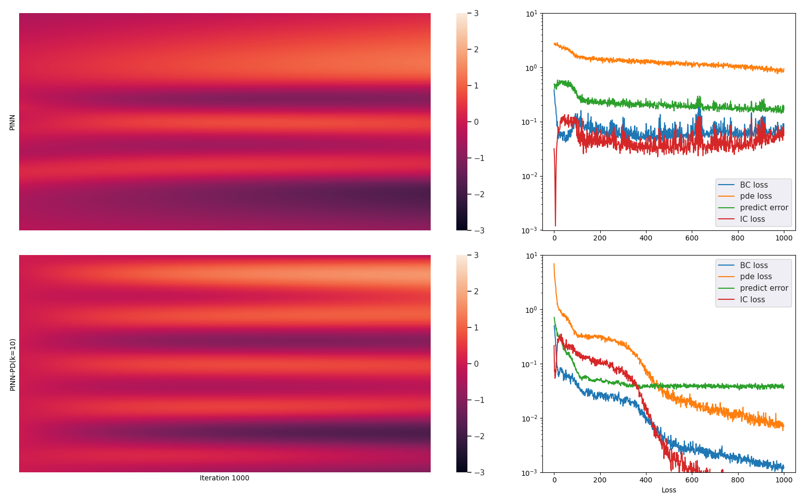
We employ $D_{10}$ with $21$ words involved. Take $N_{PDE}=1000$ inside. Note that we regard the initial value condition (16) as a boundary value conditions and take $N_{BC}=300$ . As is shown in Figure 11, the PD-PINN outperforms the PINN. As we have emphasized earlier in the manuscript, the loss curve drawn in the last subfigure suggests that the rapid vanishment of $\widehat{Loss}_{BC}$ and $\widehat{Loss}_{PDE}$ do not necessarily imply an equivalent decline of the prediction error.

References

- [1] X. Lin, Y. Rivenson, N. T. Yardimci, M. Veli, Y. Luo, M. Jarrahi, A. Ozcan, All-optical machine learning using diffractive deep neural networks, Science 361 (6406) (2018) 1004–1008.
- [2] C. H. Ding, I. Dubchak, Multi-class protein fold recognition using support vector machines and neural networks, Bioinformatics 17 (4) (2001) 349–358.
- [3] D. Wang, W. Liao, Modeling and control of magnetorheological fluid dampers using neural networks, Smart materials and structures 14 (1) (2004) 111.
- [4] Z. Long, Y. Lu, B. Dong, Pde-net 2.0: Learning pdes from data with a numeric-symbolic hybrid deep network, Journal of Computational Physics 399 (2019) 108925.
- [5] M. Raissi, P. Perdikaris, G. E. Karniadakis, Physics-informed neural networks: A deep learning framework for solving forward and inverse problems involving nonlinear partial differential equations, Journal of Computational Physics 378 (2019) 686–707.
- [6] L. Lu, X. Meng, Z. Mao, G. E. Karniadakis, Deepxde: A deep learning library for solving differential equations, arXiv preprint arXiv:1907.04502 (2019).
- [7] M. Raissi, P. Perdikaris, G. E. Karniadakis, Physics informed deep learning (part i): Data-driven solutions of nonlinear partial differential equations, arXiv preprint arXiv:1711.10561 (2017).
- [8] A. D. Jagtap, K. Kawaguchi, G. E. Karniadakis, Adaptive activation functions accelerate convergence in deep and physics-informed neural networks, Journal of Computational Physics (2020). arXiv:1906.01170, doi:10.1016/j.jcp.2019.109136.
- [9] A. D. Jagtap, K. Kawaguchi, G. E. Karniadakis, Locally adaptive activation functions with slope recovery term for deep and physics-informed neural networks, arXiv preprint arXiv:1909.12228 (2019).
- [10] J. Zhang, G. G. Walter, Y. Miao, W. N. W. Lee, Wavelet neural networks for function learning, IEEE transactions on Signal Processing 43 (6) (1995) 1485–1497.
- [11] J. D. Rairán Antolines, Reconstruction of periodic signals using neural networks, Tecnura 18 (39) (2014) 34–46.
- [12] W. Sienko, W. M. Citko, B. M. Wilamowski, Hamiltonian neural nets as a universal signal processor, in: IEEE 2002 28th Annual Conference of the Industrial Electronics Society. IECON 02, Vol. 4, IEEE, 2002, pp. 3201–3204.
- [13] J. Ling, A. Kurzawski, J. Templeton, Reynolds averaged turbulence modelling using deep neural networks with embedded invariance, Journal of Fluid Mechanics 807 (2016) 155–166.
- [14] P. Henrici, Fast fourier methods in computational complex analysis, Siam Review 21 (4) (1979) 481–527.
- [15] D. Gottlieb, S. A. Orszag, Numerical analysis of spectral methods: theory and applications, Vol. 26, Siam, 1977.
- [16] Z.-Q. J. Xu, Y. Zhang, Y. Xiao, Training behavior of deep neural network in frequency domain, in: International Conference on Neural Information Processing, Springer, 2019, pp. 264–274.
- [17] T. Luo, Z. Ma, Z.-Q. J. Xu, Y. Zhang, Theory of the frequency principle for general deep neural networks, arXiv preprint arXiv:1906.09235 (2019).
- [18] M. R. Mohammadi, E. Fatemizadeh, M. H. Mahoor, Pca-based dictionary building for accurate facial expression recognition via sparse representation, Journal of Visual Communication and Image Representation 25 (5) (2014) 1082–1092.
- [19] E. Esser, M. Moller, S. Osher, G. Sapiro, J. Xin, A convex model for nonnegative matrix factorization and dimensionality reduction on physical space, IEEE Transactions on Image Processing 21 (7) (2012) 3239–3252.
- [20] M. W. Berry, M. Browne, A. N. Langville, V. P. Pauca, R. J. Plemmons, Algorithms and applications for approximate nonnegative matrix factorization, Computational statistics & data analysis 52 (1) (2007) 155–173.
- [21] J. Mairal, F. Bach, J. Ponce, Task-driven dictionary learning, IEEE transactions on pattern analysis and machine intelligence 34 (4) (2011) 791–804.
- [22] D. Gilbarg, N. S. Trudinger, Elliptic partial differential equations of second order, springer, 2015.
- [23] A. Virmaux, K. Scaman, Lipschitz regularity of deep neural networks: analysis and efficient estimation, in: Advances in Neural Information Processing Systems, 2018, pp. 3835–3844.
- [24]
D. P. Kingma, J. Ba, Adam: A method for
stochastic optimization, in: Y. Bengio, Y. LeCun (Eds.), 3rd International
Conference on Learning Representations, ICLR 2015, San Diego, CA, USA, May
7-9, 2015, Conference Track Proceedings, 2015.
URL http://arxiv.org/abs/1412.6980 - [25] S. Y. Yee, Solution of poisson’s equation on a sphere by truncated double fourier series, Monthly Weather Review 109 (3) (1981) 501–505.
- [26] S. Maintz, M. Esser, R. Dronskowski, Efficient rotation of local basis functions using real spherical harmonics., Acta Physica Polonica B 47 (4) (2016).