跳到论文正文
W Papers独立论文阅读器 arXiv:2004.08132 论文正文 计算阅读时间 · 0%
引用这篇论文根据当前论文元数据生成,正式投稿前建议核对。


License: arXiv.org perpetual non-exclusive license
arXiv:2004.08132v2 [math.OC] 18 Nov 2020

Dividend Barrier Strategies in a Renewal Risk Model With Phase-Type Distributed Interclaim Times Note: This work was supported by National Natural Science Foundation of China Grants No. 11471171, No. 11911530091 and No. 11931018. Journal: …

Linlin Tian Email: linlin.tian@dhu.edu.cn Address: College of Science, Donghua University, Shanghai, P.R. China 201620    Zhaoyang Liu Email: liuzhy@nankai.edu.cn Corresponding author: Corresponding author Address: School of Mathematical Sciences, Nankai University, Tianjin, P.R. China 300071
Abstract

In this paper, we consider the optimal dividend problem of the renewal risk model with phase-type distributed interclaim times and exponentially distributed claim sizes. Assume that the phases of the interclaim times can be observed. We study the optimal dividend under the 2–order and the nn–order (n≥3n\geq 3)separately. In the case of 2–order phase-type distributed interclaim times, we show that the optimal dividend policy is the optimal phase-wise barrier strategy. As a byproduct, we find that in this case, the phase with higher barrier is the phase with the higher intensity to the next claim. In the case of n-order (n≥3n\geq 3) phase-type distributed interclaim times, an iteration algorithm is presented to show that the optimal phase-wise barrier strategy is optimal among all dividend policies. We also find a similar conclusion like in the case of 2–order, the phase with the highest barrier is the phase with the highest intensity to the next claim.

Keywords: 
Hamilton-Jacobi-Bellman equation , phase-type distribution , optimal dividend.
2010 MSC
60J25 , 65K10 , 91B30 , 93E20

1 Introduction

The optimal dividend problem can be traced back to De Finetti 1957. Asmussen & Taksar 1997 studied this problem when the surplus process is modeled by a Brownian motion with drift. The dividend optimization problem under the compound Poisson model is studied in Azcue & Muler 2005, Belhaj 2010 and Gerber & Shiu 2006. When the Poisson process is replaced by the renewal process, Albrecher et al. 2005 calculated the distribution of the discounted dividends for a barrier strategy when the interclaim times follow the generalized Erlang(nn)-distribution. By numerical simulation, Albrecher & Hartinger 2006 showed that the horizontal dividend barrier strategy is not necessarily optimal. Mishura and Schmidli Mishura & Schmidli 2012 showed that the phase-wise dividend barrier strategy is optimal when the interclaim times are Erlang(nn)-distributed and the claim sizes are exponentially distributed. In this paper, we will extend their work and consider a renewal risk model where the interclaim times are phase-type distributed.

For a given nn–order phase-type distributed interclaim time (n≥2n\geq 2 is a positive constant), we assume that the phases of the interclaim times can be observed. We focus on the optimal phase-wise barrier strategy. Now we introduce the definition of the phase-wise barrier strategy first. For any given phase i∈{1,2,…,n}i\in\{1,2,\ldots,n\}, we set up barriers {bi}i=1n\{b_{i}\}_{i=1}^{n} such that in any phase i,i, all capital above bib_{i} is paid as dividend, if the capital is less than the barrier bib_{i}, then the company will keep the premium until the occurrence of the next claim or reaching the given level bib_{i}. This kind of strategy is called the phase-wise barrier strategy. The optimal phase-wise barriers {bi∗}i=1n\{b_{i}^{*}\}_{i=1}^{n} is chosen among all phase-wise barriers {bi}i=1n\{b_{i}\}_{i=1}^{n} such that for any initial capital x<bi∗x<b_{i}^{*}, the cumulative discounted discounted dividend at xx attains its maximum.

By the martingale approach and some direct calculations, we get some necessary conditions for the optimal phase-wise barriers. Then we deal with the case of 22–order and n⁡(n≥3)n(n\geq 3)–order separately due to the complexity of the inverse of the n×nn\times n matrix in the case of n⁡(n≥3)n(n\geq 3)–order. Now we explain those two parts separately.

In the case of 22–order phase-type distribution, there are only two barriers b1∗,b2∗b_{1}^{*},b_{2}^{*}. If b1∗<b2∗,b_{1}^{*}<b_{2}^{*}, The interval [0,+∞)[0,+\infty) is only separated into only three parts: [0,b1∗)∪[b1∗,b2∗)∪[b2∗,+∞).[0,b_{1}^{*})\cup[b_{1}^{*},b_{2}^{*})\cup[b_{2}^{*},+\infty). We can show that the optimal phase-wise barrier strategies’ corresponding function is concave on [b1∗,+∞).[b_{1}^{*},+\infty). The way of comparing of the size of b1∗,b2∗b_{1}^{*},b_{2}^{*} can also be derived, which is the phase with the higher barrier is the phase with the higher intensity to the next claim. Mathematically speaking, the necessary condition of b1∗<b2∗b_{1}^{*}<b_{2}^{*} is λ23<λ13\lambda_{23}<\lambda_{13}, where λi​3\lambda_{i3} (i=1,2i=1,2) denotes the intensity of phase ii of entering the claim state. In the last, we can theoretically show that the optimal phase-wise barrier strategy is optimal among all admissible strategies via the HJB equation.

For the case of n⁡(n≥3)n(n\geq 3)–order distributed interclaim times, we use the numerical method to explore the optimal strategy. We bring forward a similar iteration algorithm used in Albrecher et al. 2017 and Liu et al. 2020 to show that the optimal strategy is a phase-wise barrier strategy, which is obviously the optimal phase-wise barrier strategy. The proof of the convergence of the algorithm is given. Examples of optimal phase-wise barriers are presented to illustrate the applicability of numerical methods. Interestingly, we also prove that the phase with the highest optimal barrier is the phase with the highest intensity to the next claim. This phenomenon coincides with the conclusion we get in the case of 22–order.

The whole paper is organized as follows. In Section 2, we establish the basic model and formulate the problem. In Section 3, we study the optimal phase-wise barrier and get some necessary conditions for the optimal phase-wise barriers. In Section 4, we study the case of 2–order phase-type distributed interclaim times, the optimal phase-wise barrier strategy is the optimal strategy among all dividend strategies. As a byproduct, we find that the phase with the higher barrier is the phase with the higher intensity to next claim. In Section 5, we numerically study the optimal dividend problem under the nn(n≥3n\geq 3)–order phase-type distributed interclaim times, from which we find that the optimal policy is the optimal phase-wise barrier strategy. Similar with the Section 4, we also get a conclusion that the phase with the phase with the highest optimal barrier is the phase with the highest intensity to the next claim. Some examples are given to show the application of the algorithm.

2 Models and assumption

In this section, we present the surplus process of the insurer, which includes models for aggregate claims and dividend payments to policyholders, define the value function. We work on a complete probability space (Ω,ℱ,ℙ)(\Omega,\mathscr{F},\mathbb{P}) on which all processes are well defined. The information at time tt is given by ℱt\mathscr{F}_{t}, in which {ℱt:t≥0}\{\mathscr{F}_{t}:t\geq 0\} is the complete filtration generated by the claim and the dividend processes.

The surplus process of an insurance company with dividend payments is modeled as

XtD=x+c​t−∑i=1NtYi−Dt,X_{t}^{D}=x+ct-\sum_{i=1}^{N_{t}}Y_{i}-D_{t},

where c>0c>0 is the premium rate, xx is the initial wealth, DtD_{t} is the cumulative amount of dividends paid out up to time tt. NtN_{t} is a simple counting process representing the number of the incoming claims and {Yi}\{Y_{i}\} are i.i.d. with a common distribution G⁡(x):=1−e−β​x​(β>0)G(x):=1-e^{-\beta x}(\beta>0) and independent of NtN_{t}. The interclaim times are independent and follow the phase-type distribution.

The phase-type distribution is the distribution of the life time of a terminating Markov process {Jt}t≥0\{J_{t}\}_{t\geq 0} with finitely many phases and time homogenous transition rates. More precisely, let {J¯t}t≥0\{\bar{J}_{t}\}_{t\geq 0} be a Markov process on the finite state space EΔ=E∪{Δ}E_{\Delta}=E\cup\{\Delta\}, where EE is the state space and Δ\Delta is the absorbing state. The terminating Markov process {Jt}\{J_{t}\} with state space EE and intensity matrix 𝐓\mathbf{T} is defined as the restriction to EE of {J¯t}\{\bar{J}_{t}\}. The Markov process {J¯t}t≥0\{\bar{J}_{t}\}_{t\geq 0} jumps from one state to another. All the states i∈Ei\in E are transient and once the Markov process {J¯t}\{\bar{J}_{t}\} enters the absorbing state, then it will stay in this absorbing state forever. See Asmussen & Albrecher 2010 and Bladt 2005 for more details about phase-type distribution.

In our model, the state space E:={state​ 1,state​ 2,⋯,state​n}E:=\{\mbox{state}\;1,\mbox{state}\;2,\cdots,\mbox{state}\;n\} and the Δ:=state​n+1\Delta:=\mbox{state}\;n+1, where nn is a positive constant. We call this phase-type distribution a nn-order phase-type distribution. Thus, the intensity matrix of J¯t\bar{J}_{t} has the form

𝚲=(𝐓𝐭𝟎0),\mathbf{\Lambda}=\left(\begin{array}[]{cc}\mathbf{T}&\mathbf{t}\\ \mathbf{0}&0\\ \end{array}\right),

where 𝐓\mathbf{T} is n×nn\times n dimensional matrix, 𝐭\mathbf{t} is a nn dimensional column vector and 𝟎\mathbf{0} is the nn dimensional row vector of zeros. In particular, 𝐭=−𝐓𝐞\mathbf{t}=-\mathbf{T}\mathbf{e}, where 𝐞\mathbf{e} is the n-dimensional column vector with all components equal to 11, which means, the intensity of leaving state ii equals to the sum of the intensities of leaving state ii and entering the new state jj.

The Markov process JtJ_{t} jumps from one state (or we all state as “phase") to another and stay in the state ii for an exponential time with parameter λi\lambda_{i}, 0≤i≤n,λi=−λi​i>00\leq i\leq n,\lambda_{i}=-\lambda_{ii}>0. Once it enters the absorbing state n+1n+1, the claim will occur. After the claim, the Markov chain JtJ_{t} will restart at the state i∈Ei\in E with the initial probabilities πi\pi_{i}, i=1,2⋯,ni=1,2\cdots,n. Here ∑i=1nπi=1.\sum_{i=1}^{n}\pi_{i}=1. Then it continues to jump from one state to another until the next absorption (next claim). Now we assume that the Markov process {Jt}\{J_{t}\} can be observed and is independent of the claim sizes and NN.

DtD_{t} is the cumulative amount of dividends paid out up to time tt. We say that a dividend strategy DtD_{t} is admissible if

  • 1.

    DtD_{t} is predictable, nondecreasing, ca`{\grave{\mbox{a}}}gla`{\grave{\mbox{a}}}d;

  • 2.

    The process DtD_{t} verifies Dt≤x+c​t−∑i=1NtYiD_{t}\leq x+ct-\sum_{i=1}^{N_{t}}Y_{i}.

We denote by 𝒰a​d\mathscr{U}_{ad} the set of all the admissible control strategies. For any dividend strategy DD, the expected discounted dividend payments is defined as

ViD(x)=𝔼[∫0−τ−e−δ​tdDt|J0=i,X0−D=x]\displaystyle V_{i}^{D}(x)=\mathbb{E}\left[\int_{0-}^{\tau-}e^{-\delta t}\mathrm{d}D_{t}\Big|J_{0}=i,X_{0-}^{D}=x\right]
:=𝔼i​x[∫0−τ−e−δ​tdDt],i=1,2,⋯,n,\displaystyle:=\mathbb{E}_{ix}\left[\int_{0-}^{\tau-}e^{-\delta t}\mathrm{d}D_{t}\right],\quad i=1,2,\cdots,n,

where δ>0\delta>0 is the discount factor, τ=inf{t:XtD<0}\tau=\inf\{t:X_{t}^{D}<0\} is the time of ruin. The optimal value function is defined as

Vi​(x)=supD∈𝒰a​dViD​(x),V_{i}(x)=\sup_{D\in\mathscr{U}_{ad}}V_{i}^{D}(x), (2.1)

for all x≥0x\geq 0. In the following sections, we will show that optimal dividend policy is the optimal phase-wise barrier strategy. But we will treat the case of 2–order and the n–order separately. First, we study the optimal phase-wise barrier strategy.

3 The optimal phase-wise barrier

Assume the insurance company choose a phase-wise barrier strategy, which means, they will choose a barrier bi≥0b_{i}\geq 0 for a given phase ii, i=1,2,⋯,ni=1,2,\cdots,n. If the Markov process {Jt}\{J_{t}\} is in state Jt=iJ_{t}=i, all the capital above bib_{i} is paid as a dividend. If the wealth equals to bib_{i} when Jt=iJ_{t}=i, then all the incoming premium will be paid as dividends until the next jump of JtJ_{t} occurs. Let

fiD(x)=𝔼[∫0−τ−e−δ​tdDt|J0=i,X0−D=x],i=1,2,⋯,n,f_{i}^{D}(x)=\mathbb{E}\left[\int_{0-}^{\tau-}e^{-\delta t}\mathrm{d}D_{t}\Big|J_{0}=i,X_{0-}^{D}=x\right],i=1,2,\cdots,n,

denote the phase-wise barrier strategy DD’s cumulative discounted dividends, for simplicity we omit the symbol DD if there is no confusion. For simplicity, we let fn+1​(x)=∑i=1nπi​𝔼​[fi​(x−Y)]f_{n+1}(x)=\sum_{i=1}^{n}\pi_{i}\mathbb{E}[f_{i}(x-Y)], where YY is a random variable with the distribution G⁡(⋅)G(\cdot). Now we show that the functions {fi​(x)}i=1n\{f_{i}(x)\}_{i=1}^{n} are continuously differentiable on [0,bi][0,b_{i}] and fulfill

c​fi′​(x)+∑j=1,j≠in+1λi​j​fj​(x)−(λi+δ)​fi​(x)=0,x≤bi,cf_{i}^{\prime}(x)+\sum_{j=1,j\neq i}^{n+1}\lambda_{ij}f_{j}(x)-(\lambda_{i}+\delta)f_{i}(x)=0,\quad x\leq b_{i}, (3.1)

and

fi​(x)=fi​(bi)+x−bi,x≥bi.f_{i}(x)=f_{i}(b_{i})+x-b_{i},\quad x\geq b_{i}.

Actually, for 0≤x<bi0\leq x<b_{i}, we start by considering all possible events over a very small time interval [0,h][0,h], we let hh be a small enough such that x+c​h<bix+ch<b_{i}. Conditioning on the first jump of {Jt}\{J_{t}\}, we arrive at

fi​(x)=e−δ​h​(1−λi​h)​fi​(x+c​h)+∑j=1,j≠in+1∫0he−δ​t​fj​(x+c​t)​λi​j​e−λi​t​𝑑t+o⁡(h).\displaystyle f_{i}(x)=e^{-\delta h}(1-\lambda_{i}h)f_{i}(x+ch)+\sum_{j=1,j\neq i}^{n+1}\int_{0}^{h}e^{-\delta t}f_{j}(x+ct)\lambda_{ij}e^{-\lambda_{i}t}dt+o(h). (3.2)

Upon rearrangement of (3.2), division by hh and letting h→0h\rightarrow 0 yields

c​fi′​(x)+∑j=1,j≠in+1λi​j​fj​(x)−(λi+δ)​fi​(x)=0,x≤bi.cf_{i}^{\prime}(x)+\sum_{j=1,j\neq i}^{n+1}\lambda_{ij}f_{j}(x)-(\lambda_{i}+\delta)f_{i}(x)=0,\quad x\leq b_{i}.

Although the above derivative are understood to be right-derivatives, one can apply the same arguments with x−c​hx-ch in replace of xx to find that (3.1) are also satisfied by the left-derivative. Eventually, we get that fi​(x)f_{i}(x) are continuously differentiable on [0,bi][0,b_{i}] and satisfies (3.1).

Conditioning on the first jump of {Jt}\{J_{t}\},

fi​(bi)=\displaystyle f_{i}(b_{i})= ∫0∞∫0tc​e−δ​s​𝑑s​λi​e−λi​t​𝑑t+∫0∞∑i=1,i≠jn+1λi​j​fj​(bi)​e−(λi+δ)​t​𝑑t\displaystyle\int_{0}^{\infty}\int_{0}^{t}ce^{-\delta s}\mathrm{d}s\lambda_{i}e^{-\lambda_{i}t}\mathrm{d}t+\int_{0}^{\infty}\sum_{i=1,i\neq j}^{n+1}\lambda_{ij}f_{j}(b_{i})e^{-(\lambda_{i}+\delta)t}\mathrm{d}t
=\displaystyle= c+∑i=1,i≠jn+1λi​j​fj​(bi)λi+δ.\displaystyle\frac{c+\sum_{i=1,i\neq j}^{n+1}\lambda_{ij}f_{j}(b_{i})}{\lambda_{i}+\delta}. (3.3)

Combining with (3.1), we conclude that fi′​(bi)=1.f_{i}^{\prime}(b_{i})=1.

On the other hand, we show that a solution fi​(x)f_{i}(x) to equations (3.1) on [0,bi][0,b_{i}] and fi​(x)=fi​(bi)+x−bif_{i}(x)=f_{i}(b_{i})+x-b_{i} for x>bix>b_{i} with fi′​(bi)=1f_{i}^{\prime}(b_{i})=1 is the expected cumulative discounted dividend value of the barrier strategy with barriers at bib_{i}. Consider a phase-wise barrier strategy with barriers {bi}i=1n\{b_{i}\}_{i=1}^{n} and the corresponding surplus process is denoted by XtbX_{t}^{b}. Denote the ruin time as τ.\tau. By the definition of phase-wise barrier strategy, we know that for any given phase Jt=i,i=1,2,⋯,nJ_{t}=i,i=1,2,\cdots,n, the surplus Xtb≤biX_{t}^{b}\leq b_{i}. By the Itô formula,

fJt​(Xτ∧tb)​e−δ⁡(τ∧t)=\displaystyle f_{J_{t}}(X_{\tau\wedge t}^{b})e^{-\delta(\tau\wedge t)}= fi​(x)+∫0τ∧te−δ​s​[−δ​fJs​(Xsb)+ℒ​fJs​(Xsb)]​𝑑s\displaystyle f_{i}(x)+\int_{0}^{\tau\wedge t}e^{-\delta s}[-\delta f_{J_{s}}(X_{s}^{b})+\mathscr{L}f_{J_{s}}(X_{s}^{b})]\mathrm{d}s
−∫0τ∧tfJs′(Xsb)e−δ​sdLs,\displaystyle-\int_{0}^{\tau\wedge t}{f_{J_{s}}}^{\prime}(X_{s}^{b})e^{-\delta s}\mathrm{d}L_{s},

where

ℒ​fi​(x)=c​fi′​(x)+∑j=1,j≠in+1λi​j​fj​(x)−λi​fi​(x)\mathscr{L}f_{i}(x)=c{f_{i}}^{\prime}(x)+\sum_{j=1,j\neq i}^{n+1}\lambda_{ij}{f_{j}}(x)-\lambda_{i}f_{i}(x)

is the infinitesimal generator of the process. Since XtbX_{t}^{b} follows the phase-wise barrier strategy with barriers {bi}i=1n\{b_{i}\}_{i=1}^{n}, fi​(x)f_{i}(x) solves (3.1) on [0,bi)[0,b_{i}) and fi′​(x)=1f_{i}^{\prime}(x)=1 on [bi,+∞)[b_{i},+\infty), we have that

𝔼⁡[fJt​(Xτ∧tb)​e−δ⁡(τ∧t)]=fi​(x)−𝔼⁡[∫0τ∧te−δ​s​d​Ls].\displaystyle\mathbb{E}\left[f_{J_{t}}(X_{\tau\wedge t}^{b})e^{-\delta(\tau\wedge t)}\right]=f_{i}(x)-\mathbb{E}\left[\int_{0}^{\tau\wedge t}e^{-\delta s}\mathrm{d}L_{s}\right].

Using the dominated convergence theorem and letting t→∞t\rightarrow\infty, we get that fi​(x)=𝔼⁡[∫0τe−δ​s​d​Ls]f_{i}(x)=\mathbb{E}\left[\int_{0}^{\tau}e^{-\delta s}\mathrm{d}L_{s}\right], completing the desired conclusion.

Now we try to analyse the optimal phase-wise barriers {bi}i=1n\{b_{i}\}_{i=1}^{n} such that {fi​(x)}i=1n\{f_{i}(x)\}_{i=1}^{n} become maximal for all x<bix<b_{i}. Denote the optimal phase-wise barrier as {bi∗}i=1n\{b_{i}^{*}\}_{i=1}^{n} and the corresponding value function as {fi∗}i=1n\{f_{i}^{*}\}_{i=1}^{n}. Given 1≤i≤n1\leq i\leq n and x<bi∗x<b_{i}^{*},

fi∗​(x)=\displaystyle f_{i}^{*}(x)= ∫0bi∗−xce−(λi+δ)​t​(∑j=1j≠in+1λi​j​fj∗​(x+c​t))​𝑑t+e−(λi+δ)​(bi∗−xc)​fi∗​(bi∗).\displaystyle\int_{0}^{\frac{b_{i}^{*}-x}{c}}e^{-(\lambda_{i}+\delta)t}\Bigg(\sum_{\begin{subarray}{c}j=1\\ j\neq i\end{subarray}}^{n+1}\lambda_{ij}f_{j}^{*}(x+ct)\Bigg)\mathrm{d}t+e^{-(\lambda_{i}+\delta)(\frac{b_{i}^{*}-x}{c})}f_{i}^{*}(b_{i}^{*}). (3.4)

For a given initial wealth x<bi∗x<b_{i}^{*}, consider a special strategy: paying the incoming premium as dividend until next phase jump. After the jump, follow the “optimal” phase-wise barrier strategy. Then, by the definition of the optimal phase-wise barrier strategy, we see that

fi∗​(x)\displaystyle f_{i}^{*}(x) >∫0∞(∫0tc​e−δ​s​𝑑s)​λi​e−λi​t​𝑑t+∫0∞(∑j=1j≠in+1λi​j​fj∗​(x))​e−(δ+λi)​t​𝑑t\displaystyle>\int_{0}^{\infty}\Big(\int_{0}^{t}ce^{-\delta s}\mathrm{d}s\Big)\lambda_{i}e^{-\lambda_{i}t}\mathrm{d}t+\int_{0}^{\infty}\Bigg(\sum_{\begin{subarray}{c}j=1\\ j\neq i\end{subarray}}^{n+1}\lambda_{ij}f_{j}^{*}(x)\Bigg)e^{-(\delta+\lambda_{i})t}\mathrm{d}t
=c+∑j=1,j≠in+1λi​j​fj∗​(x)λi+δ.\displaystyle=\frac{c+\sum_{j=1,j\neq i}^{n+1}\lambda_{ij}f_{j}^{*}(x)}{\lambda_{i}+\delta}. (3.5)

Combining with (3.1), we see that fi∗′​(x)>1{f_{i}^{*}}^{\prime}(x)>1 on (0,bi∗).(0,b_{i}^{*}). Now we show that fi∗′′​(bi∗)=0{f_{i}^{*}}^{\prime\prime}(b_{i}^{*})=0. Here we borrow some arguments from Mishura & Schmidli 2012. Since fi∗​(x)=fi∗​(bi∗)+x−bi∗f_{i}^{*}(x)=f_{i}^{*}(b_{i}^{*})+x-b_{i}^{*} on [bi∗,+∞)[b_{i}^{*},+\infty), fi∗′′​(bi∗+)=0{f_{i}^{*}}^{\prime\prime}(b_{i}^{*}+)=0. Thus, we only need to show that fi∗′′​(bi∗−){f_{i}^{*}}^{\prime\prime}(b_{i}^{*}-) exists and equals to 0.0. We consider a function Mi​(x)M_{i}(x) satisfies (3.1) on [0,+∞)[0,+\infty) with the boundary condition Mi​(0)=fi∗​(0)M_{i}(0)=f_{i}^{*}(0). Obviously we have Mi​(x)=fi∗​(x)M_{i}(x)=f_{i}^{*}(x) on [0,bi∗].[0,b_{i}^{*}]. We already know that Mi​(x)>1M_{i}(x)>1 for x<bi∗x<b_{i}^{*}. Suppose that Mi​(x)<1M_{i}(x)<1 for x∈(bi∗,bi∗+ε]x\in(b_{i}^{*},b_{i}^{*}+\varepsilon] for some ε>0\varepsilon>0. Suppose the Markov process JtJ_{t} start with J0=i.J_{0}=i. We consider the following strategy. First use a barrier strategy with a barrier at bi∗+εb_{i}^{*}+\varepsilon then we follow the strategy with barriers at {bi∗}i=1n\{b_{i}^{*}\}_{i=1}^{n}, except the first time we reach state ii, where we use a barrier at bi∗+εb_{i}^{*}+\varepsilon. Denote the expected cumulative discounted dividend of this strategy by f~i​(x)\tilde{f}_{i}(x). Then f~i​(x)\tilde{f}_{i}(x) solves

c​f~i′​(x)+∑j=1,j≠in+1λi​j​fj​(x)−(λi+δ)​f~i​(x)=0,x≤bi∗+ε,\displaystyle c\tilde{f}_{i}^{\prime}(x)+\sum_{j=1,j\neq i}^{n+1}\lambda_{ij}f_{j}(x)-(\lambda_{i}+\delta)\tilde{f}_{i}(x)=0,x\leq b_{i}^{*}+\varepsilon, (3.6)

and f~i′​(bi∗+ε)=1\tilde{f}_{i}^{\prime}(b_{i}^{*}+\varepsilon)=1. Further, v⁡(x)=f~i​(x)−Mi​(x)v(x)=\tilde{f}_{i}(x)-M_{i}(x) solves v′​(x)=(λi+δ)​v​(x)v^{\prime}(x)=(\lambda_{i}+\delta)v(x). Since v′​(bi∗+ε)=1−Mi′​(bi∗+ε)>0,v^{\prime}(b_{i}^{*}+\varepsilon)=1-{M_{i}}^{\prime}(b_{i}^{*}+\varepsilon)>0, we conclude that v⁡(x)>0v(x)>0 for all xx. Suppose now J0≠iJ_{0}\neq i. If we now follow the strategy with barriers at {bi∗}i=1n\{b_{i}^{*}\}_{i=1}^{n}, except the first time we reach state ii, where we use a barrier at bi∗+εb_{i}^{*}+\varepsilon, we get a higher value. In the same way, we find that using a barrier at bi∗+εb_{i}^{*}+\varepsilon the first two times state ii is visited, a higher value is reached. Proceeding in the same way, we find that a barrier at bi∗+εb_{i}^{*}+\varepsilon instead of bi∗b_{i}^{*} would give a larger expected cumulative discounted dividend value. Since we have assumed that the barrier bi∗b_{i}^{*} is chosen optimally, it contradicts the assumption of Mi′​(x)≤1M_{i}^{\prime}(x)\leq 1. Eventually we see that Mi′​(x)≥1M_{i}^{\prime}(x)\geq 1 in an environment of bi∗.b_{i}^{*}. Eventually, we see that fi∗′​(x){f_{i}^{*}}^{\prime}(x) attains its minimum at bi∗b_{i}^{*}, which shows that fi∗′′​(bi∗)=0.{f_{i}^{*}}^{\prime\prime}(b_{i}^{*})=0.

Now we summarize the above two necessary conditions for the optimal phase-wise barrier {bi∗}i=1n\{b_{i}^{*}\}_{i=1}^{n}:

  1. 1.

    fi∗′​(x)>1{f_{i}^{*}}^{\prime}(x)>1 on (0,bi∗),i=1,2​…,n.(0,b_{i}^{*}),i=1,2\ldots,n.

  2. 2.

    fi∗′′​(bi∗)=0.{f_{i}^{*}}^{\prime\prime}(b_{i}^{*})=0.

Different with Mishura & Schmidli 2012, we can not solve the optimal phase-wise barrier strategy’s value function directly due to the parameter complexity. Thus, we will treat the case of 2–order and nn–order separately. In summary, in the case of 2–order phase-type distributed interclaim times, we theoretically show the the optimal phase-wise barrier strategy is optimal among all dividend policies. In the case of nn–order, we use the numerical way to show the same conclusion.

4 2-order phase-type distributed interclaim times

4.1 The concavity

Theorem 4.1.

If 0<b1∗<b2∗0<b_{1}^{*}<b_{2}^{*}, then the optimal phase-wise barrier strategy’s value function f2∗​(x)f_{2}^{*}(x) is concave on [b1∗,+∞).[b_{1}^{*},+\infty).

Proof.

Recall that fi∗​(x)f_{i}^{*}(x), i=1,2i=1,2, satisfy the equations

c​f1∗′​(x)+λ12​f2∗​(x)−(λ1+δ)​f1∗​(x)+λ13​β​e−β​x​∫0xeβ​y​(π1​f1∗​(y)+π2​f2∗​(y))​dy=0,x∈[0,b1∗];c{f_{1}^{*}}^{\prime}(x)+\lambda_{12}f_{2}^{*}(x)-(\lambda_{1}+\delta)f_{1}^{*}(x)+\lambda_{13}\beta e^{-\beta x}\int_{0}^{x}e^{\beta y}(\pi_{1}f_{1}^{*}(y)+\pi_{2}f_{2}^{*}(y))\mathrm{d}y=0,\\ x\in[0,b_{1}^{*}]; (4.1)
c​f2∗′​(x)+λ21​f1∗​(x)−(λ2+δ)​f2∗​(x)+λ23​β​e−β​x​∫0xeβ​y​(π1​f1∗​(y)+π2​f2∗​(y))​dy=0,x∈[0,b2∗].c{f_{2}^{*}}^{\prime}(x)+\lambda_{21}f_{1}^{*}(x)-(\lambda_{2}+\delta)f_{2}^{*}(x)+\lambda_{23}\beta e^{-\beta x}\int_{0}^{x}e^{\beta y}(\pi_{1}f_{1}^{*}(y)+\pi_{2}f_{2}^{*}(y))\mathrm{d}y=0,\\ x\in[0,b_{2}^{*}]. (4.2)
f1∗​(x)=f1∗​(b1∗)+x−b1∗,\displaystyle f_{1}^{*}(x)=f_{1}^{*}(b_{1}^{*})+x-b_{1}^{*},\quad x∈(b1∗,+∞).\displaystyle x\in(b_{1}^{*},+\infty).
f2∗​(x)=f2∗​(b2∗)+x−b2∗,\displaystyle f_{2}^{*}(x)=f_{2}^{*}(b_{2}^{*})+x-b_{2}^{*},\quad x∈(b2∗,+∞).\displaystyle x\in(b_{2}^{*},+\infty).

Taking the derivative in (4.2), we get

c​f2∗′′​(x)+λ21​f1∗′​(x)+(β​c−(λ2+δ))​f2∗′​(x)+β⁡(λ23​π1+λ21)​f1∗​(x)+β(λ23π2−(λ2+δ))f2∗(x)=0,x∈[0,b2∗).c{f_{2}^{*}}^{\prime\prime}(x)+\lambda_{21}{f_{1}^{*}}^{\prime}(x)+(\beta c-(\lambda_{2}+\delta)){f_{2}^{*}}^{\prime}(x)+\beta(\lambda_{23}\pi_{1}+\lambda_{21}){f_{1}^{*}}(x)\\ +\beta(\lambda_{23}\pi_{2}-(\lambda_{2}+\delta))f_{2}^{*}(x)=0,\qquad x\in[0,{b_{2}^{*}}). (4.3)

Using f1∗′​(x)=1{f_{1}^{*}}^{\prime}(x)=1,

c​f2∗′′′​(x)+(c​β−(λ2+δ))​f2∗′′​(x)+β⁡(λ23​π2−(λ2+δ))​f2∗′​(x)+β(λ23π1+λ21)=0,x∈[b1∗,b2∗).c{f_{2}^{*}}^{\prime\prime\prime}(x)+(c\beta-(\lambda_{2}+\delta)){f_{2}^{*}}^{\prime\prime}(x)+\beta(\lambda_{23}\pi_{2}-(\lambda_{2}+\delta)){f_{2}^{*}}^{\prime}(x)\\ +\beta(\lambda_{23}\pi_{1}+\lambda_{21})=0,\qquad x\in[{b_{1}^{*}},{b_{2}^{*}}). (4.4)

Suppose there exists a point x∈[b1∗,b2∗)x\in[{b_{1}^{*}},{b_{2}^{*}}) such that f2∗′′​(x)>0{f_{2}^{*}}^{\prime\prime}(x)>0. If c​β−(λ2+δ)≤0c\beta-(\lambda_{2}+\delta)\leq 0, then

c​f2∗′′′​(x)≥−β⁡(λ23​π1+λ21)+β⁡(λ2+δ−λ23​π2)​f2∗′​(x).\displaystyle c{f_{2}^{*}}^{\prime\prime\prime}(x)\geq-\beta(\lambda_{23}\pi_{1}+\lambda_{21})+\beta(\lambda_{2}+\delta-\lambda_{23}\pi_{2}){f_{2}^{*}}^{\prime}(x).

Since f2∗′​(x)>1{f_{2}^{*}}^{\prime}(x)>1 on [b1∗,b2∗)[{b_{1}^{*}},{b_{2}^{*}}), we see that c​f2∗′′′​(x)>β​δc{f_{2}^{*}}^{\prime\prime\prime}(x)>\beta\delta. Thus, f2∗′′​(x)>0{f_{2}^{*}}^{\prime\prime}(x)>0 on (x,b2∗](x,{b_{2}^{*}}], contradicting that f2∗′′​(b2∗)=0{f_{2}^{*}}^{\prime\prime}({b_{2}^{*}})=0. If c​β−(λ2+δ)>0c\beta-(\lambda_{2}+\delta)>0, taking the derivative in (4.4),

c​f2∗′′′′​(x)+(c​β−(λ2+δ))​f2∗′′′​(x)+β⁡(λ23​π2−(λ2+δ))​f2∗′′​(x)=0.c{f_{2}^{*}}^{\prime\prime\prime\prime}(x)+(c\beta-(\lambda_{2}+\delta)){f_{2}^{*}}^{\prime\prime\prime}(x)+\beta(\lambda_{23}\pi_{2}-(\lambda_{2}+\delta)){f_{2}^{*}}^{\prime\prime}(x)=0.

Because f2∗′′​(b2∗)=0{f_{2}^{*}}^{\prime\prime}({b_{2}^{*}})=0, the solution of f2∗′′​(x){f_{2}^{*}}^{\prime\prime}(x) is of the form

f2∗′′​(x)=A⁡(er1​(x−b2∗)−er2​(x−b2∗)),{f_{2}^{*}}^{\prime\prime}(x)=A(e^{r_{1}(x-{b_{2}^{*}})}-e^{r_{2}(x-{b_{2}^{*}})}),

where r2<0<r1r_{2}<0<r_{1} are the two roots of

c​r2+(c​β−(λ2+δ))​r+β⁡(λ23​π2−(λ2+δ))=0.cr^{2}+(c\beta-(\lambda_{2}+\delta))r+\beta(\lambda_{23}\pi_{2}-(\lambda_{2}+\delta))=0.

From the assumption that f2∗′′​(x)>0{f_{2}^{*}}^{\prime\prime}(x)>0 for some x∈[b1∗,b2∗),x\in[{b_{1}^{*}},{b_{2}^{*}}), we conclude that A<0A<0. Thus, f2∗′′​(x)>0{f_{2}^{*}}^{\prime\prime}(x)>0 for all x∈[b1∗,b2∗)x\in[{b_{1}^{*}},{b_{2}^{*}}). Then we have f2∗′​(x)<1{f_{2}^{*}}^{\prime}(x)<1 for x∈[b1∗,b2∗)x\in[{b_{1}^{*}},{b_{2}^{*}}), yielding a contradiction. Until now, we show that for all x∈[b1∗,b2∗),x\in[{b_{1}^{*}},{b_{2}^{*}}), f2∗′′​(x)≤0{f_{2}^{*}}^{\prime\prime}(x)\leq 0. Because f2∗​(x)=f2∗​(b2∗)+x−b2∗{f_{2}^{*}}(x)={f_{2}^{*}}({b_{2}^{*}})+x-{b_{2}^{*}} for x>b2∗x>{b_{2}^{*}}, we find that f2∗​(x)f_{2}^{*}(x) is concave on [b1∗,+∞)[{b_{1}^{*}},+\infty). ∎

4.2 The Optimality

In this section, we will show that the optimal phase-wise barrier dividend strategy is optimal among all strategies when the interclaim times follow the 2-order phase-type distribution.

Theorem 4.2.

If the interclaim times follow a 2-order phase-type distribution, then the optimal phase-wise barrier strategy’s value function fi∗​(x)f_{i}^{*}(x) satisfies the following Hamilton-Jacobi-Bellman (HJB) equation

max{cfi∗′(x)+∑j=1,j≠i3λi​jfj∗(x)−(λi+δ)fi∗(x),1−fi∗′(x)}=0,i=1,2,\max\Big\{c{f_{i}^{*}}^{\prime}(x)+\sum_{j=1,j\neq i}^{3}\lambda_{ij}f_{j}^{*}(x)-(\lambda_{i}+\delta){f_{i}^{*}}(x),1-{f_{i}^{*}}^{\prime}(x)\Big\}=0,\quad i=1,2, (4.5)

where f3∗​(x)=β​e−β​x​∫0xeβ​y​(π1​f1∗​(y)+π2​f2∗​(y))​𝑑y{f_{3}^{*}}(x)=\beta e^{-\beta x}\int_{0}^{x}e^{\beta y}(\pi_{1}{f_{1}^{*}}(y)+\pi_{2}{f_{2}^{*}}(y))\mathrm{d}y.

Proof.

Since for all x>bi∗x>b_{i}^{*}, fi∗​(x)=fi∗​(bi∗)+x−bi∗{f_{i}^{*}}(x)={f_{i}^{*}}(b_{i}^{*})+x-b_{i}^{*}, i=1,2i=1,2 and for all 0≤x<bi∗,0\leq x<b_{i}^{*}, fi∗​(x){f_{i}^{*}}(x) satisfies (4.1) and (4.2), we only need to show that

c​fi∗′​(x)+∑j=1,j≠i3λi​j​fj∗​(x)−(λi+δ)​fi∗​(x)≤0c{f_{i}^{*}}^{\prime}(x)+\sum_{j=1,j\neq i}^{3}\lambda_{ij}f_{j}^{*}(x)-(\lambda_{i}+\delta){f_{i}^{*}}(x)\leq 0

on [bi∗,+∞)[b_{i}^{*},+\infty). We will prove

c​f1∗′​(x)+∑j=23λ1​j​fj∗​(x)−(λ1+δ)​f1∗​(x)≤0c{f_{1}^{*}}^{\prime}(x)+\sum_{j=2}^{3}\lambda_{1j}{f_{j}^{*}}(x)-(\lambda_{1}+\delta){f_{1}^{*}}(x)\leq 0

on [b1∗,+∞)[{b_{1}^{*}},+\infty) first. Multiplying by eβ​xe^{\beta x} gives

c​f1∗′​(x)​eβ​x+λ12​eβ​x​f2∗​(x)+λ13​β​∫0xeβ​y​(π1​f1∗​(y)+π2​f2∗​(y))​𝑑y−(δ+λ1)​eβ​x​f1∗​(x).c{f_{1}^{*}}^{\prime}(x)e^{\beta x}+\lambda_{12}e^{\beta x}{f_{2}^{*}}(x)+\lambda_{13}\beta\int_{0}^{x}e^{\beta y}(\pi_{1}{f_{1}^{*}}(y)+\pi_{2}{f_{2}^{*}}(y))\mathrm{d}y-(\delta+\lambda_{1})e^{\beta x}{f_{1}^{*}}(x).

Taking the derivative yields

eβ​x​[λ12​f2∗′​(x)+(λ12​β+λ13​π2)​f2∗​(x)+(λ13​π1​β−β⁡(δ+λ1))​f1∗​(x)+c​β−(δ+λ1)]=:eβ​x​g1​(x).e^{\beta x}\big[\lambda_{12}{f_{2}^{*}}^{\prime}(x)+(\lambda_{12}\beta+\lambda_{13}\pi_{2}){f_{2}^{*}}(x)+(\lambda_{13}\pi_{1}\beta-\beta(\delta+\lambda_{1})){f_{1}^{*}}(x)+c\beta-(\delta+\lambda_{1})\big]\\ =:e^{\beta x}g_{1}(x).

Noticing that g1​(b1∗)=0g_{1}({b_{1}^{*}})=0, we only need to show that

g1′​(x)=λ12​f2∗′′​(x)+β⁡(λ12+λ13​π2)​f2∗′​(x)+β⁡(λ13​π1−(δ+λ1))≤0,x∈[b1∗,+∞).g_{1}^{\prime}(x)=\lambda_{12}{f_{2}^{*}}^{\prime\prime}(x)+\beta(\lambda_{12}+\lambda_{13}\pi_{2}){f_{2}^{*}}^{\prime}(x)+\beta(\lambda_{13}\pi_{1}-(\delta+\lambda_{1}))\leq 0,\\ x\in[{b_{1}^{*}},+\infty).

Since f2∗​(x){f_{2}^{*}}(x) is concave on [b1∗,+∞),[{b_{1}^{*}},+\infty), we only need to show that

(λ12+λ13​π2)​f2∗′​(b1)≤δ+λ1−λ13​π1.(\lambda_{12}+\lambda_{13}\pi_{2}){f_{2}^{*}}^{\prime}(b_{1})\leq\delta+\lambda_{1}-\lambda_{13}\pi_{1}. (4.6)

Recall that

c​f1∗′​(x)+λ12​f2∗​(x)+λ13​f3∗​(x)−(λ1+δ)​f1∗​(x)=0,x∈(0,b1∗].c{f_{1}^{*}}^{\prime}(x)+\lambda_{12}f_{2}^{*}(x)+\lambda_{13}f_{3}^{*}(x)-(\lambda_{1}+\delta)f_{1}^{*}(x)=0,x\in(0,b_{1}^{*}]. (4.7)

Taking the derivative of (4.7), we see that

λ12​f2∗′​(b1)+λ13​f3∗′​(b1)−(λ1+δ)=0.\lambda_{12}{f_{2}^{*}}^{\prime}(b_{1})+\lambda_{13}{f_{3}^{*}}^{\prime}(b_{1})-(\lambda_{1}+\delta)=0. (4.8)

Combining (4.6) with (4.7), we only need to show that

f3∗′​(b1)≥π1+π2​f2∗′​(b1).{f_{3}^{*}}^{\prime}(b_{1})\geq\pi_{1}+\pi_{2}{f_{2}^{*}}^{\prime}(b_{1}). (4.9)

On the other hand,

c​f2∗′​(x)+λ21​f1∗​(x)+λ23​f3∗​(x)−(λ2+δ)​f2∗​(x)=0,x∈(0,b2].c{f_{2}^{*}}^{\prime}(x)+\lambda_{21}f_{1}^{*}(x)+\lambda_{23}f_{3}^{*}(x)-(\lambda_{2}+\delta)f_{2}^{*}(x)=0,x\in(0,b_{2}]. (4.10)

Taking the derivative of (4.10),

c​f2∗′′​(x)+λ21​f1∗′​(x)+λ23​f3∗′​(x)−(λ2+δ)​f2∗′​(x)=0,x∈(0,b2].c{f_{2}^{*}}^{\prime\prime}(x)+\lambda_{21}{f_{1}^{*}}^{\prime}(x)+\lambda_{23}{f_{3}^{*}}^{\prime}(x)-(\lambda_{2}+\delta){f_{2}^{*}}^{\prime}(x)=0,x\in(0,b_{2}].

Since f2∗f_{2}^{*} is concave on [b1,b2][b_{1},b_{2}] and f1∗′​(b1)=1{f_{1}^{*}}^{\prime}(b_{1})=1,

λ21​f1∗′​(b1)+λ23​f3∗′​(b1)−(λ2+δ)​f2∗′​(b1)≥0,\lambda_{21}{f_{1}^{*}}^{\prime}(b_{1})+\lambda_{23}{f_{3}^{*}}^{\prime}(b_{1})-(\lambda_{2}+\delta){f_{2}^{*}}^{\prime}(b_{1})\geq 0,

After simplification,

f3∗′​(b1)≥(λ2+δ)​f2∗′​(b1)λ23.{f_{3}^{*}}^{\prime}(b_{1})\geq\frac{(\lambda_{2}+\delta){f_{2}^{*}}^{\prime}(b_{1})}{\lambda_{23}}. (4.11)

Now we compare the right-hand side of both (4.9) and (4.11). Using the fact that f2∗′​(b1)≥1{f_{2}^{*}}^{\prime}(b_{1})\geq 1, we can easily obtain that

f3∗′​(b1)≥(λ2+δ)​f2∗′​(b1)λ23≥π1+π2​f2∗′​(b1).{f_{3}^{*}}^{\prime}(b_{1})\geq\frac{(\lambda_{2}+\delta){f_{2}^{*}}^{\prime}(b_{1})}{\lambda_{23}}\geq\pi_{1}+\pi_{2}{f_{2}^{*}}^{\prime}(b_{1}).

Until now, we show that (4.9) holds, eventually

cf1∗′(x)+∑j=23λ1​jfj∗(x)−(λ1+δ)f1∗(x)≤0,x∈[b1∗,+∞).c{f_{1}^{*}}^{\prime}(x)+\sum_{j=2}^{3}\lambda_{1j}{f_{j}^{*}}(x)-(\lambda_{1}+\delta){f_{1}^{*}}(x)\leq 0,\quad x\in[{b_{1}^{*}},+\infty).

Now we show that

cf2∗′(x)+λ21f1∗(x)+λ23f3∗(x)−(λ2+δ)f2∗(x)≤0,x∈[b2∗,+∞).c{f_{2}^{*}}^{\prime}(x)+\lambda_{21}{f_{1}^{*}}(x)+\lambda_{23}{f_{3}^{*}}(x)-(\lambda_{2}+\delta){f_{2}^{*}}(x)\leq 0,\quad x\in[{b_{2}^{*}},+\infty).

Multiplying by eβ​xe^{\beta x} gives

c​eβ​x​f2∗′​(x)+λ21​eβ​x​f1∗​(x)+λ23​β​∫0xeβ​y​(π1​f1∗​(y)+π1​f2∗​(y))​𝑑y−(λ2+δ)​eβ​x​f2∗​(x).ce^{\beta x}{f_{2}^{*}}^{\prime}(x)+\lambda_{21}e^{\beta x}{f_{1}^{*}}(x)+\lambda_{23}\beta\int_{0}^{x}e^{\beta y}(\pi_{1}{f_{1}^{*}}(y)+\pi_{1}{f_{2}^{*}}(y))dy-(\lambda_{2}+\delta)e^{\beta x}{f_{2}^{*}}(x).

Taking the derivative yields

eβ​x​(c​β+λ21​β​f1∗​(x)+λ21+λ23​β​(π1​f1∗​(x)+π2​f2∗​(x))−(λ2+δ)​β​f2∗​(x)−(λ2+δ))=:eβ​x​g2​(x),e^{\beta x}(c\beta+\lambda_{21}\beta{f_{1}^{*}}(x)+\lambda_{21}+\lambda_{23}\beta(\pi_{1}{f_{1}^{*}}(x)+\pi_{2}{f_{2}^{*}}(x))-(\lambda_{2}+\delta)\beta{f_{2}^{*}}(x)-(\lambda_{2}+\delta))\\ =:e^{\beta x}g_{2}(x),

here we use that f2∗′′​(x)=0{f_{2}^{*}}^{\prime\prime}(x)=0, f1∗′​(x)=1{f_{1}^{*}}^{\prime}(x)=1 on [b2∗,+∞)[{b_{2}^{*}},+\infty). Since g2​(b2∗)=0g_{2}({b_{2}^{*}})=0 and

g2′​(x)=λ21​β+λ23​β−(λ2+δ)​β<0,g_{2}^{\prime}(x)=\lambda_{21}\beta+\lambda_{23}\beta-(\lambda_{2}+\delta)\beta<0,

we see that eβ​x​g2​(x)≤0e^{\beta x}g_{2}(x)\leq 0 on [b2∗,+∞)[{b_{2}^{*}},+\infty). Combining this with

c​f2∗′​(b1∗)+λ21​f1∗​(b1∗)+λ23​f3∗​(b1∗)−(λ2+δ)​f2∗​(b1∗)=0,c{f_{2}^{*}}^{\prime}({b_{1}^{*}})+\lambda_{21}{f_{1}^{*}}({b_{1}^{*}})+\lambda_{23}{f_{3}^{*}}({b_{1}^{*}})-(\lambda_{2}+\delta){f_{2}^{*}}({b_{1}^{*}})=0,

we see that

cf2∗′(x)+λ21f1∗(x)+λ23f3∗(x)−(λ2+δ)f2∗(x)≤0,x∈[b2∗,+∞).c{f_{2}^{*}}^{\prime}(x)+\lambda_{21}{f_{1}^{*}}(x)+\lambda_{23}{f_{3}^{*}}(x)-(\lambda_{2}+\delta){f_{2}^{*}}(x)\leq 0,\quad x\in[{b_{2}^{*}},+\infty).

Until now, we show that the optimal phase-wise barrier strategy’s value function satisfies the HJB equation. ∎

Theorem 4.3.

For exponential distributed claim sizes and 2-order phase-type distributed interclaim times, the optimal phase-wise barrier strategy is the optimal policy among all dividend strategies.

Proof.

Clearly fi∗​(x)≤Vi​(x)f_{i}^{*}(x)\leq V_{i}(x), where Vi​(x)V_{i}(x) is defined in (2.1). Let LtL_{t} be an arbitrary dividend process and XtLX_{t}^{L} denote the corresponding surplus process. Then by Itô’s formula,

fJt∗​(Xτ∧tL)​e−δ⁡(τ∧t)=\displaystyle f_{J_{t}}^{*}(X_{\tau\wedge t}^{L})e^{-\delta(\tau\wedge t)}= fi∗​(x)+∫0τ∧te−δ​s​[−δ​fJs∗​(XsL)+ℒ​fJs∗​(XsL)]​𝑑s\displaystyle f_{i}^{*}(x)+\int_{0}^{\tau\wedge t}e^{-\delta s}[-\delta f_{J_{s}}^{*}(X_{s}^{L})+\mathscr{L}f_{J_{s}}^{*}(X_{s}^{L})]\mathrm{d}s
−∫0τ∧tfJs∗′(XsL)e−δ​sdLs,\displaystyle-\int_{0}^{\tau\wedge t}{f_{J_{s}}^{*}}^{\prime}(X_{s}^{L})e^{-\delta s}\mathrm{d}L_{s},

where τ\tau is the ruin time and

ℒ​fi∗​(x)=c​fi∗′​(x)+∑j=1,j≠i3λi​j​fj∗​(x)−λi​fi∗​(x)\mathscr{L}f_{i}^{*}(x)=c{f_{i}^{*}}^{\prime}(x)+\sum_{j=1,j\neq i}^{3}\lambda_{ij}{f_{j}^{*}}(x)-\lambda_{i}f_{i}^{*}(x)

is the infinitesimal generator of the process. From (4.5) we conclude that

𝔼⁡[fJt∗​(Xτ∧tL)​e−δ⁡(τ∧t)]\displaystyle\mathbb{E}\left[f_{J_{t}}^{*}(X_{\tau\wedge t}^{L})e^{-\delta(\tau\wedge t)}\right] ≤fi∗(x)−𝔼[∫0τ∧tfJs∗′(XsL)e−δ​sdLs|J0=i,X0−L=x]\displaystyle\leq f_{i}^{*}(x)-\mathbb{E}\left[\int_{0}^{\tau\wedge t}{f_{J_{s}}^{*}}^{\prime}(X_{s}^{L})e^{-\delta s}\mathrm{d}L_{s}\Big|J_{0}=i,X_{0-}^{L}=x\right]
≤fi∗(x)−𝔼[∫0τ∧te−δ​sdLs|J0=i,X0−L=x].\displaystyle\leq f_{i}^{*}(x)-\mathbb{E}\left[\int_{0}^{\tau\wedge t}e^{-\delta s}\mathrm{d}L_{s}\Big|J_{0}=i,X_{0-}^{L}=x\right].

Letting t→∞t\rightarrow\infty gives

fi∗(x)≥𝔼[∫0τe−δ​sdLs|J0=i,X0−L=x].f_{i}^{*}(x)\geq\mathbb{E}\left[\int_{0}^{\tau}e^{-\delta s}\mathrm{d}L_{s}\Big|J_{0}=i,X_{0-}^{L}=x\right].

Since the strategy LtL_{t} is arbitrary, fi∗​(x)≥Vi​(x)f_{i}^{*}(x)\geq V_{i}(x). Now we complete the proof. ∎

Until now, we see that the 2–layer barrier dividend strategy is optimal when the interclaim times follow 2–order phase–type distribution. In what follows, we will find a way to compare the those two barriers.

4.3 The comparison of two optimal barriers

Theorem 4.4.

If 0<b1∗<b2∗0<{b_{1}^{*}}<{b_{2}^{*}}, then λ23>λ13\lambda_{23}>\lambda_{13}.

Proof.

Denote f3∗​(x)=β​e−β​x​∫0xeβ​y​(∑i=12πi​fi∗​(y))​𝑑y{f_{3}^{*}}(x)=\beta e^{-\beta x}\int_{0}^{x}e^{\beta y}(\sum_{i=1}^{2}\pi_{i}f_{i}^{*}(y))\mathrm{d}y. From (4.2), we see that

c​f2∗′′​(x)+λ21−(λ2+δ)​f2∗′​(x)+λ23​f3∗′​(x)=0,x∈[b1∗,b2∗].c{f_{2}^{*}}^{\prime\prime}(x)+\lambda_{21}-(\lambda_{2}+\delta){f_{2}^{*}}^{\prime}(x)+\lambda_{23}{f_{3}^{*}}^{\prime}(x)=0,x\in[{b_{1}^{*}},{b_{2}^{*}}].

Combining the concavity of f2∗​(x){f_{2}^{*}}(x) on [b1∗,b2∗][{b_{1}^{*}},{b_{2}^{*}}], we see

λ21−(λ2+δ)​f2∗′​(b1∗)+λ23​f3∗′​(b1∗)≥0.\lambda_{21}-(\lambda_{2}+\delta){f_{2}^{*}}^{\prime}({b_{1}^{*}})+\lambda_{23}{f_{3}^{*}}^{\prime}({b_{1}^{*}})\geq 0. (4.12)

On the other hand, from (4.1),

λ12​f2∗′​(b1∗)+λ13​f3∗′​(b1∗)−(λ1+δ)=0.\lambda_{12}{f_{2}^{*}}^{\prime}({b_{1}^{*}})+\lambda_{13}{f_{3}^{*}}^{\prime}({b_{1}^{*}})-(\lambda_{1}+\delta)=0. (4.13)

Combining (4.12) with (4.13), we see that

f2∗′​(b1∗)≤λ13​λ21+(λ1+δ)​λ23(λ2+δ)​λ13+λ23​λ12.{f_{2}^{*}}^{\prime}({b_{1}^{*}})\leq\frac{\lambda_{13}\lambda_{21}+(\lambda_{1}+\delta)\lambda_{23}}{(\lambda_{2}+\delta)\lambda_{13}+\lambda_{23}\lambda_{12}}. (4.14)

Since f2∗′​(b1∗)>1{f_{2}^{*}}^{\prime}({b_{1}^{*}})>1, we know λ13​λ21+(λ1+δ)​λ23(λ2+δ)​λ13+λ23​λ12>1.\frac{\lambda_{13}\lambda_{21}+(\lambda_{1}+\delta)\lambda_{23}}{(\lambda_{2}+\delta)\lambda_{13}+\lambda_{23}\lambda_{12}}>1. After simplification, we see that λ23>λ13\lambda_{23}>\lambda_{13}. ∎

The above theorem shows that when the interclaim times are 2–order phase-type distributed, the phase with the higher barrier must be the phase with the higher intensity to claim.

Now we show some numerical examples for the case of 2–order phase-type distributed interclaim times. The algorithm is shown in the next section.

Example 4.5.

Let the interclaim times follow a 2-order phase-type distribution. The state 33 is the absorption state of the Markov process {Jt}\{J_{t}\}, which means, once the Markov process enters the state 3, the claim occurs. The intensity matrix 𝚲\mathbf{\Lambda} is

(−λ1λ12λ13λ21−λ2λ23)=(−10554−128).\left(\begin{array}[]{ccc}-\lambda_{1}&\lambda_{12}&\lambda_{13}\\ \lambda_{21}&-\lambda_{2}&\lambda_{23}\\ \end{array}\right)=\left(\begin{array}[]{ccc}-10&5&5\\ 4&-12&8\\ \end{array}\right).

And c=15c=15, δ=0.1\delta=0.1, β=1\beta=1, (π1,π2)=(0.4,0.6)(\pi_{1},\pi_{2})=(0.4,0.6). Table 1 shows b1∗<b2∗b_{1}^{*}<b_{2}^{*}.

Phase ii 1 2
Optimal phase-wise barrier bi∗b_{i}^{*} 11.779 12.219
Table 1: bi∗b^{*}_{i} for a 2-order case with λ23>λ13\lambda_{23}>\lambda_{13}.

The functions f1∗​(x)f_{1}^{*}(x) and f2∗​(x)f_{2}^{*}(x) are shown in Figure 2.

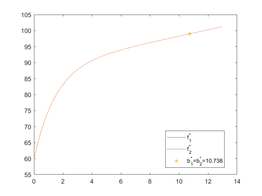
Another numerical experiment for 2-order case is shown next for what happens if the intensity to the next claim is the same.

Example 4.6.

Let the interclaim times follow a 2-order phase-type distribution, and c=15c=15, δ=0.1\delta=0.1, β=1\beta=1, (π1,π2)=(0.4,0.6)(\pi_{1},\pi_{2})=(0.4,0.6). The intensity matrix 𝚲\mathbf{\Lambda} is

(−λ1λ12λ13λ21−λ2λ23)=(−8351−65),\left(\begin{array}[]{ccc}-\lambda_{1}&\lambda_{12}&\lambda_{13}\\ \lambda_{21}&-\lambda_{2}&\lambda_{23}\\ \end{array}\right)=\left(\begin{array}[]{ccc}-8&3&5\\ 1&-6&5\\ \end{array}\right),
State ii 1 2
Optimal phase-wise barrier bi∗b_{i}^{*} 10.738 10.738
Table 2: bi∗b^{*}_{i} for a 2-order case with λ13=λ23\lambda_{13}=\lambda_{23}.

From Table 2, we see that the barriers are the same. The equality of f1∗​(x)f_{1}^{*}(x) and f2∗​(x)f_{2}^{*}(x) is shown in the Figure 2.

Refer to caption
Figure 1: fi∗​(x)f_{i}^{*}(x) for λ23>λ13\lambda_{23}>\lambda_{13}.
Refer to caption
Figure 2: fi∗​(x)f_{i}^{*}(x) for λ13=λ23\lambda_{13}=\lambda_{23}.
Remark 4.7.

When the interclaim times are 2-order phase-type distributed, we can also compare the size of the barrier by comparing different phases’ the expected time to the next claim. Recall that for a given phase ii, the expected time of the next claim 𝒯i\mathcal{T}_{i} is, confer Asmussen & Albrecher 2010 (Page 256, Theorem 1.5-(d)),

𝒯i=αi​𝐓−1​𝐞,\mathcal{T}_{i}=\alpha_{i}\mathbf{T}^{-1}\mathbf{e}, (4.15)

where αi=(0,0,⋯,0,−1,0,⋯,0)\alpha_{i}=(0,0,\cdots,0,-1,0,\cdots,0) is an nn-dimensional vector with −1-1 being the iith term, 𝐓\mathbf{T} is the subintensity matrix of 𝚲\mathbf{\Lambda} restricted to EE and 𝐞\mathbf{e} is the column vector with all components equal to one.

If λ23≥λ13\lambda_{23}\geq\lambda_{13}, then

𝒯1−𝒯2\displaystyle\mathcal{T}_{1}-\mathcal{T}_{2} =(−11)⋅𝐓−1⋅(11)\displaystyle=\Big(\begin{array}[]{cc}-1&1\\ \end{array}\Big)\cdot\mathbf{T}^{-1}\cdot\left(\begin{array}[]{c}1\\ 1\end{array}\right)
=1λ1​λ2−λ12​λ21​(−11)⋅(−λ2−λ12−λ21−λ1)\displaystyle=\frac{1}{\lambda_{1}\lambda_{2}-\lambda_{12}\lambda_{21}}\Big(\begin{array}[]{cc}-1&1\\ \end{array}\Big)\cdot\left(\begin{array}[]{c}-\lambda_{2}-\lambda_{12}\\ -\lambda_{21}-\lambda_{1}\end{array}\right)
=1λ1​λ2−λ12​λ21​(λ23−λ13)≥0.\displaystyle=\frac{1}{\lambda_{1}\lambda_{2}-\lambda_{12}\lambda_{21}}(\lambda_{23}-\lambda_{13})\geq 0.

Eventually, combining this with Theorem 4.4, we get that if 0<b1∗<b2∗0<{b_{1}^{*}}<{b_{2}^{*}}, then 𝒯1≥𝒯2\mathcal{T}_{1}\geq\mathcal{T}_{2}, which shows that for different phases, except by comparing the intensity to the claim to compare the size of barriers, we can also compare the expected time to the next claim to obtain which barrier is larger.

5 n-order (n≥3n\geq 3) phase-type distributed interclaim times

Since there are too many parameters in the case of nn–order (n≥3)(n\geq 3), a similar calculation like Theorem 4.1 is almost impossible. Thus, we numerically explore the optimal policy. We present an algorithm first and then we show that the convergence of the algorithm. By the numerical exploration, we get that the optimal phase-wise barrier strategy is optimal among all admissible dividend policies.

5.1 Algorithm

We use the iteration algorithm which is similar with the ones used in Albrecher et al. 2017 and Liu et al. 2020.

  1. 1.

    Set k=0k=0 and initialize with Vi(0)≡0V^{(0)}_{i}\equiv 0, i=1,2,⋯,n+1i=1,2,\cdots,n+1.

  2. 2.

    Set k=k+1k=k+1. For given Vi(k−1)V_{i}^{(k-1)}, we look for the optimal dividend strategy prior to τ1=inf{t≥0:J¯t≠J0}\tau_{1}=\inf\{t\geq 0:\bar{J}_{t}\neq J_{0}\} with terminal cost,

    Vi(k)(x)=supD∈𝒰a​d𝔼[∫0−τ1−e−δ​tdDt+e−δ​τ1VJ¯τ1(k−1)(Xτ1D)|J0=i,X0−D=x]V_{i}^{(k)}(x)=\sup_{D\in\mathscr{U}_{ad}}\mathbb{E}\Big[\int_{0-}^{\tau_{1}-}e^{-\delta t}\mathrm{d}D_{t}+e^{-\delta\tau_{1}}V_{\bar{J}_{\tau_{1}}}^{(k-1)}(X^{D}_{\tau_{1}})\Big|J_{0}=i,X^{D}_{0-}=x\Big] (5.1)

    for i=1,2,⋯,ni=1,2,\cdots,n. The corresponding HJB equation is

    max⁡{c​Vi(k)′​(x)−(λi+δ)​Vi(k)​(x)+∑j=1,j≠in+1λi​j​Vj(k−1)​(x),1−Vi(k)′​(x)}=0.\max\Big\{c{V_{i}^{(k)}}^{\prime}(x)-(\lambda_{i}+\delta){V_{i}^{(k)}}(x)+\sum_{j=1,j\neq i}^{n+1}\lambda_{ij}V_{j}^{(k-1)}(x),1-{V_{i}^{(k)}}^{\prime}(x)\Big\}=0. (5.2)
  3. 3.

    If max⁡supx≥0i⁡|Vi(k)​(x)−Vi(k−1)​(x)|<tolerance\max_{i}\sup_{x\geq 0}|V_{i}^{(k)}(x)-V_{i}^{(k-1)}(x)|<\textrm{tolerance} for k>1k>1 stop; otherwise, go to Step 2.

Actually, in Step 2, we find that the optimal strategy is a phase-wise barrier strategy with barriers

bi(k)=arg⁡maxx≥0{c+∑j=1,j≠in+1λi​j​Vj(k−1)​(x)λi+δ−x},i=1,2,⋯,n.b_{i}^{(k)}=\mathop{\arg\max}_{x\geq 0}\left\{\frac{c+\sum_{j=1,j\neq i}^{n+1}\lambda_{ij}V_{j}^{(k-1)}(x)}{\lambda_{i}+\delta}-x\right\},\quad i=1,2,\cdots,n. (5.3)

And the corresponding functions Vi(k)V_{i}^{(k)} are obtained by

Vi(k)​(x)={e−λi+δc​(bi(k)−x)​Vi(k)​(bi(k))+1c∫xbi(k)e−λi+δc​(u−x)(∑j=1j≠in+1λi​jVj(k−1)(u))du,x<bi(k);c+∑j=1,j≠in+1λi​j​Vj(k−1)​(x)λi+δ,x=bi(k);Vi(k)​(bi(k))+x−bi(k),x>bi(k),V_{i}^{(k)}(x)=\begin{cases}\displaystyle e^{-\frac{\lambda_{i}+\delta}{c}(b_{i}^{(k)}-x)}V_{i}^{(k)}(b_{i}^{(k)})&\\ \displaystyle\quad+\frac{1}{c}\int_{x}^{b_{i}^{(k)}}e^{-\frac{\lambda_{i}+\delta}{c}(u-x)}\Big(\sum_{\begin{subarray}{c}j=1\\ j\neq i\end{subarray}}^{n+1}\lambda_{ij}V_{j}^{(k-1)}(u)\Big)\mathrm{d}u,&x<b_{i}^{(k)};\\ \displaystyle\frac{c+\sum_{j=1,j\neq i}^{n+1}\lambda_{ij}V_{j}^{(k-1)}(x)}{\lambda_{i}+\delta},&x=b_{i}^{(k)};\\ V_{i}^{(k)}(b_{i}^{(k)})+x-b_{i}^{(k)},&x>b_{i}^{(k)},\\ \end{cases} (5.4)

for i=1,2,⋯,ni=1,2,\cdots,n, and

Vn+1(k)​(x)=β​e−β​x​∫0xeβ​y​(∑i=1nπi​Vi(k)​(y))​𝑑y.V_{n+1}^{(k)}(x)=\beta e^{-\beta x}\int_{0}^{x}e^{\beta y}\left(\sum_{i=1}^{n}\pi_{i}V_{i}^{(k)}(y)\right)\mathrm{d}y. (5.5)

After we present the algorithm, we show the convergence of the algorithm. The proof contains two parts, the first part (more specifically, Proposition 5.2)proves that {Vi(k)}i=1n\{V_{i}^{(k)}\}_{i=1}^{n} converges to the optimal value function {Vi}i=1n\{V_{i}\}_{i=1}^{n}, the second part (Proposition 5.3) proves that iteration strategy {bi(k)}i=1n\{b_{i}^{(k)}\}_{i=1}^{n} convergence to the optimal policy {bi∗}i=1n\{b_{i}^{*}\}_{i=1}^{n}.

5.2 The convergence of the algorithm

Lemma 5.1.

We have Vi(0)≤Vi(1)≤⋯≤Vi(k)≤⋯≤ViV_{i}^{(0)}\leq V_{i}^{(1)}\leq\cdots\leq V_{i}^{(k)}\leq\cdots\leq V_{i} for i=1,2,⋯,ni=1,2,\cdots,n.

Proof.

We prove the result by induction.

(i) It follows from Vi(0)≡0V_{i}^{(0)}\equiv 0 that the optimal strategy is barrier strategy with bi(1)=0b_{i}^{(1)}=0, i.e.,

Vi(1)(x)=supD∈𝒰a​d𝔼[∫0−τ1−e−δ​tdDt|J0=i,X0−D=x]=x+cλi+δ.V_{i}^{(1)}(x)=\sup_{D\in\mathscr{U}_{ad}}\mathbb{E}\Big[\int_{0-}^{\tau_{1}-}e^{-\delta t}\mathrm{d}D_{t}\Big|J_{0}=i,X^{D}_{0-}=x\Big]=x+\frac{c}{\lambda_{i}+\delta}. (5.6)

We have Vi(0)≤Vi(1)V_{i}^{(0)}\leq V_{i}^{(1)}.

(ii) Assume that Vi(k−2)≤Vi(k−1)V_{i}^{(k-2)}\leq V_{i}^{(k-1)}. By (5.1), we have

Vi(k)​(x)≥\displaystyle V_{i}^{(k)}(x)\geq supD∈𝒰a​d𝔼[∫0−τ1−e−δ​tdDt+e−δ​τ1VJ¯τ1(k−2)(Xτ1D)|J0=i,X0−D=x]\displaystyle\sup_{D\in\mathscr{U}_{ad}}\mathbb{E}\Big[\int_{0-}^{\tau_{1}-}e^{-\delta t}\mathrm{d}D_{t}+e^{-\delta\tau_{1}}V_{\bar{J}_{\tau_{1}}}^{(k-2)}(X^{D}_{\tau_{1}})\Big|J_{0}=i,X^{D}_{0-}=x\Big]
=\displaystyle= Vi(k−1)​(x).\displaystyle V_{i}^{(k-1)}(x).

∎

Proposition 5.2.

It holds that Vi(k)→ViV_{i}^{(k)}\to V_{i} as k→∞k\to\infty for i=1,2,⋯,ni=1,2,\cdots,n.

Proof.

For any admissible strategy D∈𝒰a​dD\in\mathscr{U}_{ad}, we have

Dt≤x+c​t.D_{t}\leq x+ct.

Then

Vi​(x)=supD∈𝒰a​dViD​(x)≤x+∫0∞c​e−δ​t​𝑑t=x+cδ.V_{i}(x)=\sup_{D\in\mathscr{U}_{ad}}V_{i}^{D}(x)\leq x+\int_{0}^{\infty}ce^{-\delta t}\mathrm{d}t=x+\frac{c}{\delta}.

So there exists T>0T>0 such that

e−δ​t​Vi​(x+c​t)​<13​εfort>​T.e^{-\delta t}V_{i}(x+ct)<\frac{1}{3}\varepsilon\quad\hbox{for}\quad t>T. (5.7)

Let us define K=mini⁡Vi​(x+p​T)K=\min_{i}V_{i}(x+pT) and take N>0N>0 such that

ℙ{τN≥T}≥1−ε3​K.\mathbb{P}\{\tau_{N}\geq T\}\geq 1-\frac{\varepsilon}{3K}. (5.8)

There exists an admissible strategy Dε∈𝒰a​dD^{\varepsilon}\in\mathscr{U}_{ad} such that

Vi​(x)−ViDε​(x)<13​ε.V_{i}(x)-V_{i}^{D^{\varepsilon}}(x)<\frac{1}{3}\varepsilon. (5.9)

Denote τN\tau_{N} the Nt​hN^{th} jump time of the Markov process {Jt}\{J_{t}\} (The claim counts as one jump). We define the strategy DND^{N} as DtN=DtεD^{N}_{t}=D^{\varepsilon}_{t} for t≤τN∧τt\leq\tau_{N}\land\tau, and DtN=DτNεD^{N}_{t}=D^{\varepsilon}_{\tau_{N}} for t>τNt>\tau_{N} if τN<τ\tau_{N}<\tau. From (5.7) and (5.8), we have

ViDε​(x)−ViDN​(x)\displaystyle V_{i}^{D^{\varepsilon}}(x)-V_{i}^{D^{N}}(x)
=\displaystyle= 𝔼i​x​[∫τN∧τ−τ−e−δ​t​d​Dtε]≤𝔼i​x​[e−δ⁡(τN∧τ)​VJ¯τN∧τ​(XτN∧τDε)]\displaystyle\mathbb{E}_{ix}\Big[\int_{\tau_{N}\land\tau-}^{\tau-}e^{-\delta t}\mathrm{d}D^{\varepsilon}_{t}\Big]\leq\mathbb{E}_{ix}\Big[e^{-\delta(\tau_{N}\land\tau)}V_{\bar{J}_{\tau_{N}\land\tau}}(X^{D^{\varepsilon}}_{\tau_{N}\land\tau})\Big]
≤\displaystyle\leq 𝔼i​x[𝟏{τN∧τ≥T}e−δ⁡(τN∧τ)VJ¯τN∧τ(x+c(τN∧τ))]\displaystyle\mathbb{E}_{ix}\Big[\mathbf{1}_{\{\tau_{N}\land\tau\geq T\}}e^{-\delta(\tau_{N}\land\tau)}V_{\bar{J}_{\tau_{N}\land\tau}}(x+c(\tau_{N}\land\tau))\Big]
+𝔼i​x[𝟏{τN≤T}VJ¯τN∧τ(x+c(τN∧τ))]\displaystyle+\mathbb{E}_{ix}\Big[\mathbf{1}_{\{\tau_{N}\leq T\}}V_{\bar{J}_{\tau_{N}\land\tau}}(x+c(\tau_{N}\land\tau))\Big]
≤\displaystyle\leq 𝔼i​x[𝟏{τN∧τ≥T}e−δ⁡(τN∧τ)VJ¯τN∧τ(x+c(τN∧τ))]+Kℙ{τN<T}\displaystyle\mathbb{E}_{ix}\Big[\mathbf{1}_{\{\tau_{N}\land\tau\geq T\}}e^{-\delta(\tau_{N}\land\tau)}V_{\bar{J}_{\tau_{N}\land\tau}}(x+c(\tau_{N}\land\tau))\Big]+K\mathbb{P}\{\tau_{N}<T\}
<\displaystyle< 23​ε.\displaystyle\frac{2}{3}\varepsilon.

The we obtain from (5.9),

Vi​(x)≤ViDε​(x)+13​ε<ViDN​(x)+ε.V_{i}(x)\leq V_{i}^{D^{\varepsilon}}(x)+\frac{1}{3}\varepsilon<V_{i}^{D^{N}}(x)+\varepsilon. (5.10)

If we define a sequence of strategies D1,D2,⋯,DN−1D^{1},D^{2},\cdots,D^{N-1} as Dtk=DτN−k+tND^{k}_{t}=D^{N}_{\tau_{N-k}+t}, we can see that

ViDk​(x)=𝔼i​x​[∫0−τ1−e−δ​t​d​Dtk+e−δ​τ1​VJ¯τ1Dk−1​(Xτ1Dk)]fork=1,⋯,NV_{i}^{D^{k}}(x)=\mathbb{E}_{ix}\Big[\int_{0-}^{\tau_{1}-}e^{-\delta t}\mathrm{d}D^{k}_{t}+e^{-\delta\tau_{1}}V_{\bar{J}_{\tau_{1}}}^{D^{k-1}}(X^{D^{k}}_{\tau_{1}})\Big]\quad\hbox{for}\quad k=1,\cdots,N

with ViD0=V(0)≡0V_{i}^{D^{0}}=V^{(0)}\equiv 0. These imply that ViD1​(x)≤Vi(1)​(x)V_{i}^{D^{1}}(x)\leq V_{i}^{(1)}(x). Assume that ViDk−1​(x)≤Vi(k−1)​(x)V_{i}^{D^{k-1}}(x)\leq V_{i}^{(k-1)}(x). We have

ViDk​(x)=\displaystyle V_{i}^{D^{k}}(x)= 𝔼i​x​[∫0−τ1−e−δ​t​d​Dtk+e−δ​τ1​VJ¯τ1Dk−1​(Xτ1Dk)]\displaystyle\mathbb{E}_{ix}\Big[\int_{0-}^{\tau_{1}-}e^{-\delta t}\mathrm{d}D^{k}_{t}+e^{-\delta\tau_{1}}V_{\bar{J}_{\tau_{1}}}^{D^{k-1}}(X^{D^{k}}_{\tau_{1}})\Big]
≤\displaystyle\leq 𝔼i​x​[∫0−τ1−e−δ​t​d​Dtk+e−δ​τ1​VJ¯τ1(k−1)​(Xτ1Dk)]≤Vi(k)​(x).\displaystyle\mathbb{E}_{ix}\Big[\int_{0-}^{\tau_{1}-}e^{-\delta t}\mathrm{d}D^{k}_{t}+e^{-\delta\tau_{1}}V_{\bar{J}_{\tau_{1}}}^{(k-1)}(X^{D^{k}}_{\tau_{1}})\Big]\leq V_{i}^{(k)}(x).

Hence we obtain

ViDN​(x)≤Vi(N)​(x).V_{i}^{D^{N}}(x)\leq V_{i}^{(N)}(x).

Following from (5.10) and Lemma 5.1, we have

Vi​(x)<Vi(N)​(x)+ε≤Vi(k)​(x)+εfork>N.V_{i}(x)<V_{i}^{(N)}(x)+\varepsilon\leq V_{i}^{(k)}(x)+\varepsilon\quad\hbox{for}\quad k>N.

On the other hand, we have Vi​(x)≥Vi(k)​(x)V_{i}(x)\geq V_{i}^{(k)}(x). This completes the proof. ∎

Proposition 5.3.

The optimal value function ViV_{i} is the minimal nonnegative solution of the equation

Vi(x)=supD∈𝒰a​d𝔼[∫0−τ1−e−δ​tdDt+e−δ​τ1VJ¯τ1(Xτ1D)|J0=i,X0−D=x].V_{i}(x)=\sup_{D\in\mathscr{U}_{ad}}\mathbb{E}\Big[\int_{0-}^{\tau_{1}-}e^{-\delta t}\mathrm{d}D_{t}+e^{-\delta\tau_{1}}V_{\bar{J}_{\tau_{1}}}(X^{D}_{\tau_{1}})\Big|J_{0}=i,X^{D}_{0-}=x\Big]. (5.11)

If there exists an optimal phase-wise barrier strategy with {bi∗}i=1n\{b_{i}^{*}\}_{i=1}^{n} prior to τ1\tau_{1} for the problem (5.1) after replacing Vi(k−1)V_{i}^{(k-1)} by ViV_{i}, then the phase-wise barrier strategy with {bi∗}i=1n\{b_{i}^{*}\}_{i=1}^{n} is optimal for the optimization problem (2.1).

Proof.

The dynamic programming principle implies that the optimal value function ViV_{i} is a nonnegative solution of (5.11). On the other hand, let WiW_{i} be a nonnegative solution of (5.11), the Wi≥Vi(0)≡0W_{i}\geq V_{i}^{(0)}\equiv 0. Assume that Wi≥Vi(k−1)W_{i}\geq V_{i}^{(k-1)}. We have

Wi​(x)=\displaystyle W_{i}(x)= supD∈𝒰a​d𝔼i​x​[∫0−τ1−e−δ​t​d​Dt+e−δ​τ1​WJ¯τ1​(Xτ1D)]\displaystyle\sup_{D\in\mathscr{U}_{ad}}\mathbb{E}_{ix}\Big[\int_{0-}^{\tau_{1}-}e^{-\delta t}\mathrm{d}D_{t}+e^{-\delta\tau_{1}}W_{\bar{J}_{\tau_{1}}}(X^{D}_{\tau_{1}})\Big]
≥\displaystyle\geq supD∈𝒰a​d𝔼i​x​[∫0−τ1−e−δ​t​d​Dt+e−δ​τ1​VJ¯τ1(k−1)​(Xτ1D)]=Vi(k)​(x).\displaystyle\sup_{D\in\mathscr{U}_{ad}}\mathbb{E}_{ix}\Big[\int_{0-}^{\tau_{1}-}e^{-\delta t}\mathrm{d}D_{t}+e^{-\delta\tau_{1}}V_{\bar{J}_{\tau_{1}}}^{(k-1)}(X^{D}_{\tau_{1}})\Big]=V_{i}^{(k)}(x).

Hence, Wi≥Vi(k)W_{i}\geq V_{i}^{(k)} for all k≥0k\geq 0. It follows from Vi(k)→ViV_{i}^{(k)}\to V_{i} that Wi≥ViW_{i}\geq V_{i}. These conclude that ViV_{i} is the minimal nonnegative solution of (5.11).

Suppose that the phase-wise barrier strategy D∗D^{*} with {bi∗}i=1n\{b_{i}^{*}\}_{i=1}^{n} is the optimal strategy prior to τ1\tau_{1}. Then

Vi​(x)=𝔼i​x​[∫0−τ1−e−δ​t​d​Dt∗+e−δ​τ1​VJ¯τ1​(Xτ1D∗)].V_{i}(x)=\mathbb{E}_{ix}\Big[\int_{0-}^{\tau_{1}-}e^{-\delta t}\mathrm{d}D^{*}_{t}+e^{-\delta\tau_{1}}V_{\bar{J}_{\tau_{1}}}(X^{D^{*}}_{\tau_{1}})\Big].

We have by induction that

Vi​(x)=𝔼i​x​[∫0−τn−e−δ​t​d​Dt∗+e−δ​τn​VJ¯τn​(XτnD∗)]V_{i}(x)=\mathbb{E}_{ix}\Big[\int_{0-}^{\tau_{n}-}e^{-\delta t}\mathrm{d}D^{*}_{t}+e^{-\delta\tau_{n}}V_{\bar{J}_{\tau_{n}}}(X^{D^{*}}_{\tau_{n}})\Big]

for all n≥1n\geq 1. In view of that 𝔼i​x​[e−δ​τn​VJ¯τn]→0\mathbb{E}_{ix}[e^{-\delta\tau_{n}}V_{\bar{J}_{\tau_{n}}}]\to 0 as n→∞n\to\infty, and letting n→∞n\to\infty, we have

Vi​(x)=𝔼i​x​[∫0−τ−e−δ​t​d​Dt∗].V_{i}(x)=\mathbb{E}_{ix}\Big[\int_{0-}^{\tau-}e^{-\delta t}\mathrm{d}D^{*}_{t}\Big].

∎

5.3 Examples

In what follows, we show some examples.

Example 5.4.

Let the interclaims follow a 3-order phase-type distribution. The intensity matrix 𝐓\mathbf{T} is

(−λ1λ12λ13λ14λ21−λ2λ23λ24λ31λ32−λ3λ34)=(−105232−124624−82),\left(\begin{array}[]{cccc}-\lambda_{1}&\lambda_{12}&\lambda_{13}&\lambda_{14}\\ \lambda_{21}&-\lambda_{2}&\lambda_{23}&\lambda_{24}\\ \lambda_{31}&\lambda_{32}&-\lambda_{3}&\lambda_{34}\\ \end{array}\right)=\left(\begin{array}[]{cccc}-10&5&2&3\\ 2&-12&4&6\\ 2&4&-8&2\\ \end{array}\right),

c=21.4c=21.4, δ=0.1\delta=0.1, β=1\beta=1, (π1,π2,π3)=(0.2,0.3,0.5)(\pi_{1},\pi_{2},\pi_{3})=(0.2,0.3,0.5). Table 3 shows that phase 2 has the highest barrier.

Phase ii 1 2 3
The intenisty to the next claim λi​4\lambda_{i4} 3 6 2
Optimal phase-wise barriers bi∗b_{i}^{*} 9.61 10.26 9.27
Table 3: bi∗b_{i}^{*} for a 3-order case with (π1,π2,π3)=(0.2,0.3,0.5)(\pi_{1},\pi_{2},\pi_{3})=(0.2,0.3,0.5).

The functions fi∗​(x)f_{i}^{*}(x) are shown in Figure 3.

Refer to caption
Figure 3: fi∗​(x)f_{i}^{*}(x) for Example 5.4.

If the initial probabilities (π1,π2,π3)=(0.2,0.3,0.5)(\pi_{1},\pi_{2},\pi_{3})=(0.2,0.3,0.5) are replaced by (0.1,0.1,0.8)(0.1,0.1,0.8), the new barriers are shown in Table 4. As we can see, phase 2 still has the highest barrier.

Phase ii 1 2 3
Optimal phase-wise barrier bi∗b_{i}^{*} 9.39 10.03 9.05
Table 4: bi∗b_{i}^{*} for a 3-order case with (π1,π2,π3)=(0.1,0.1,0.8)(\pi_{1},\pi_{2},\pi_{3})=(0.1,0.1,0.8).
Example 5.5.

Let the interclaim times follow a 4-order phase-type distribution, and c=25c=25, δ=0.1\delta=0.1, β=1\beta=1, (π1,π2,π3,π4)=(0.5,0.2,0.2,0.1)(\pi_{1},\pi_{2},\pi_{3},\pi_{4})=(0.5,0.2,0.2,0.1). The intensity matrix 𝐓\mathbf{T} is

(−λ1λ12λ13λ14λ15λ21−λ2λ23λ24λ25λ31λ32−λ3λ34λ35λ41λ42λ43−λ4λ45)=(−1052123−1443422−1271231−60).\left(\begin{array}[]{ccccc}-\lambda_{1}&\lambda_{12}&\lambda_{13}&\lambda_{14}&\lambda_{15}\\ \lambda_{21}&-\lambda_{2}&\lambda_{23}&\lambda_{24}&\lambda_{25}\\ \lambda_{31}&\lambda_{32}&-\lambda_{3}&\lambda_{34}&\lambda_{35}\\ \lambda_{41}&\lambda_{42}&\lambda_{43}&-\lambda_{4}&\lambda_{45}\\ \end{array}\right)=\left(\begin{array}[]{ccccc}-10&5&2&1&2\\ 3&-14&4&3&4\\ 2&2&-12&7&1\\ 2&3&1&-6&0\\ \end{array}\right).

The optimal phase-wise barriers are shown in Table 5. In this case, we can see that phase 2 has the highest barrier.

Phase ii 1 2 3 4
The intensity to the next claim λi​5\lambda_{i5} 2 4 1 0
Optimal phase-wise barrier bi∗b_{i}^{*} 8.907 9.554 8.274 7.106
Table 5: bi∗b_{i}^{*} for a 4-order case
Refer to caption
Figure 4: fi∗​(x)f_{i}^{*}(x) for Example 5.5.
Example 5.6.

Let us try another example with phase 1 and phase 4 having the same highest intensity. c=25c=25, δ=0.1\delta=0.1, β=1\beta=1, (π1,π2,π3,π4)=(0.5,0.2,0.2,0.1)(\pi_{1},\pi_{2},\pi_{3},\pi_{4})=(0.5,0.2,0.2,0.1). The intensity matrix 𝐓\mathbf{T} is

(−λ1λ12λ13λ14λ15λ21−λ2λ23λ24λ25λ31λ32−λ3λ34λ35λ41λ42λ43−λ4λ45)=(−1673154−812101−412000−55).\left(\begin{array}[]{ccccc}-\lambda_{1}&\lambda_{12}&\lambda_{13}&\lambda_{14}&\lambda_{15}\\ \lambda_{21}&-\lambda_{2}&\lambda_{23}&\lambda_{24}&\lambda_{25}\\ \lambda_{31}&\lambda_{32}&-\lambda_{3}&\lambda_{34}&\lambda_{35}\\ \lambda_{41}&\lambda_{42}&\lambda_{43}&-\lambda_{4}&\lambda_{45}\\ \end{array}\right)=\left(\begin{array}[]{ccccc}-16&7&3&1&5\\ 4&-8&1&2&1\\ 0&1&-4&1&2\\ 0&0&0&-5&5\\ \end{array}\right).

The optimal phase-wise barriers are shown in Table 6. In this example, the phase 1 and phase 4 have the same highest intensity to the next claim and phase 1, 4 have the same highest barrier.

State ii 1 2 3 4
The intensity to the next claim λi​5\lambda_{i5} 5 1 2 5
Optimal phase-wise barrier bi∗b_{i}^{*} 10.109 8.805 9.205 10.109
Table 6: bi∗b_{i}^{*} with two same highest intensity
Refer to caption
Figure 5: fi∗​(x)f_{i}^{*}(x) for Example 5.6.
Example 5.7.

Let use try another example with the same intensity to the next claim. c=21c=21, δ=0.1\delta=0.1, β=1\beta=1, (π1,π2,π3,π4)=(0.5,0.2,0.2,0.1)(\pi_{1},\pi_{2},\pi_{3},\pi_{4})=(0.5,0.2,0.2,0.1). The intensity matrix 𝐓\mathbf{T} is

(−λ1λ12λ13λ14λ15λ21−λ2λ23λ24λ25λ31λ32−λ3λ34λ35λ41λ42λ43−λ4λ45)=(−1673154−1212501−715113−105).\left(\begin{array}[]{ccccc}-\lambda_{1}&\lambda_{12}&\lambda_{13}&\lambda_{14}&\lambda_{15}\\ \lambda_{21}&-\lambda_{2}&\lambda_{23}&\lambda_{24}&\lambda_{25}\\ \lambda_{31}&\lambda_{32}&-\lambda_{3}&\lambda_{34}&\lambda_{35}\\ \lambda_{41}&\lambda_{42}&\lambda_{43}&-\lambda_{4}&\lambda_{45}\\ \end{array}\right)=\left(\begin{array}[]{ccccc}-16&7&3&1&5\\ 4&-12&1&2&5\\ 0&1&-7&1&5\\ 1&1&3&-10&5\\ \end{array}\right).

The optimal phase-wise barriers are shown in Table 7. In this example, all phases have the same highest intensity to the next claim and all phases have the same highest barrier. The figure in 6 shows that the value of f1∗​(x),f2∗​(x),f3∗​(x),f4∗​(x)f_{1}^{*}(x),f_{2}^{*}(x),f_{3}^{*}(x),f_{4}^{*}(x) equals to each other.

Phase ii 1 2 3 4
The intensity to the next claim 5 5 5 5
Optimal phase-wise barrier bi∗b_{i}^{*} 10.611 10.611 10.611 10.611
Table 7: bi∗b_{i}^{*} with the same highest intensity
Refer to caption
Figure 6: fi∗​(x)f_{i}^{*}(x) for Example 5.7.

5.4 The phase with the highest barrier has the highest intensity to the claim

From the above numerical experiments, an interesting phenomenon can be brought out:

Proposition 5.8.

The phase with the the highest barrier must be the phase with highest intensity to the next claim.

Until now, we know that the optimal phase-wise barrier strategy is optimal among all admissible policies, not just the case of 2–order phase-type distribution. Thus, the phase-wise optimal barrier strategy’s corresponding value function solves the following HJB equation

max{cfi∗(x)+∑j=1,j≠in+1λi​jfj∗(x)−(λi+δ)fi∗(x),1−fi∗′(x)}=0,i=1,…,n,\max\left\{cf_{i}^{*}(x)+\sum_{j=1,j\neq i}^{n+1}\lambda_{ij}f_{j}^{*}(x)-(\lambda_{i}+\delta)f_{i}^{*}(x),1-{f_{i}^{*}}^{\prime}(x)\right\}=0,i=1,\ldots,n,

where fn+1∗​(x)=∑i=1nπi​𝔼​[fi​(x−Y)]f_{n+1}^{*}(x)=\sum_{i=1}^{n}\pi_{i}\mathbb{E}[f_{i}(x-Y)]. Without loss of generality, we assume that 0<b1<b2<…<bn0<b_{1}<b_{2}<\ldots<b_{n}. At x=bnx=b_{n},

c​fi∗′′​(bn)+∑j=1,j≠in+1λi​j​fj∗′​(bn)−(λi+δ)​fi∗′​(bn)≤0,i<n.c{f_{i}^{*}}^{\prime\prime}(b_{n})+\sum_{j=1,j\neq i}^{n+1}\lambda_{ij}{f_{j}^{*}}^{\prime}(b_{n})-(\lambda_{i}+\delta){f_{i}^{*}}^{\prime}(b_{n})\leq 0,\quad i<n. (5.12)
c​fn∗′′​(bn)+∑j=1,j≠nn+1λn​j​fj∗′​(bn)−(λn+δ)​fn∗′​(bn)=0.c{f_{n}^{*}}^{\prime\prime}(b_{n})+\sum_{j=1,j\neq n}^{n+1}\lambda_{nj}{f_{j}^{*}}^{\prime}(b_{n})-(\lambda_{n}+\delta){f_{n}^{*}}^{\prime}(b_{n})=0. (5.13)

Notice that for all i≤n,i\leq n, fi∗′​(bn)=1{f_{i}^{*}}^{\prime}(b_{n})=1 and fi∗′′​(bn)=0{f_{i}^{*}}^{\prime\prime}(b_{n})=0. Combining this with (5.12), we get that

fn+1∗′​(bn)≤1+δλi,n+1,i<n.{f_{n+1}^{*}}^{\prime}(b_{n})\leq 1+\frac{\delta}{\lambda_{i,n+1}},\quad i<n. (5.14)

On the other hand, by (5.13), we get that

fn+1∗′​(bn)=1+δλn,n+1.{f_{n+1}^{*}}^{\prime}(b_{n})=1+\frac{\delta}{\lambda_{n,n+1}}. (5.15)

Combining (5.14) and (5.15), we get that λi,n+1≤λn,n+1\lambda_{i,n+1}\leq\lambda_{n,n+1}. Eventually, we get that the nthn^{\mbox{th}} phase has the highest intensity to the next claim, which verifies that the phase with the highest barrier has the highest intensity to the next claim.

6 Conclusion

In this paper, we study the optimal dividend problem when the interclaim times follow the nn–order (n≥2CLOSE(n\geq 2) phase type distribution. By direct calculation, we theoretically prove that the optimal strategy is a phase-wise barrier strategy in the case of 2–order distributed interclaim times. On the other hand, for the case of nn–order distributed interclaim times, since there are two many parameters in the matrix, the direct calculation is impossible. We bring up a numerical algorithm to show the optimality of the phase-wise barrier strategy.

About the optimal barrier’s size comparison of different phases, we also find that in the case of n⁡(n≥3)n(n\geq 3)–order, the phase with the highest is the phase with the highest intensity to the next claim, which coincides with the same conclusion in the case of 22–order.

Acknowledgements

Part of this work was done when the first author were visiting Professor Hansjörg Albrecher. Thanks for his inspiration and guidance.

References

  • Albrecher et al. (2017) Albrecher, H., Azcue, P., & Muler, N. (2017). Optimal dividend strategies for two collaborating insurance companies. Advances in Applied Probability, 49(2), 515–548.
  • Albrecher et al. (2005) Albrecher, H., Claramunt, M.M., & Mármol, M. (2005). On the distribution of dividend payments in a Sparre Andersen model with generalized Erlang(n) interclaim times. Insurance: Mathematics and Economics, 37(2 SPEC. ISS.), 324–334.
  • Albrecher & Hartinger (2006) Albrecher, H., & Hartinger, J. (2006). On the non-optimality of horizontal barrier strategies in the Sparre Andersen model. Hermis Journal of Computer Mathematics and Its Applications, 7, 109–122.
  • Asmussen & Albrecher (2010) Asmussen, S., & Albrecher, H. (2010). Ruin Probabilities (Second Edition). New Jersey: World Scientific.
  • Asmussen & Taksar (1997) Asmussen, S., & Taksar, M. (1997). Controlled diffusion models for optimal dividend pay-out. Insurance: Mathematics and Economics, 20(1), 1–15.
  • Azcue & Muler (2005) Azcue, P., Muler, N. (2005). Optimal reinsurance and dividend distribution policies in the Cramér-Lundberg model. Mathematical Finance, 15(2), 261–308.
  • Belhaj (2010) Belhaj, M. (2010). Optimal dividend payments when cash reserves follow a jump-diffusion process. Mathematical Finance, 20(2), 313–325.
  • Bladt (2005) Bladt, M. (2005). A review on phase-type distributions and their use in risk theory. Astin Bulletin, 35(1), 145–161.
  • De Finetti (1957) De Finetti, B. (1957). Su un’ impostazione alternativa dell teoria collettiva del rischio. In: Transactions of the XVth International Congress of Actuaries, New York, (II), 433–443.
  • Gerber & Shiu (2006) Gerber, H.U., & Shiu, E.S.W. (2006). On optimal dividend strategies in the compound Poisson model. North American Actuarial Journal, 10(2), 76–93.
  • Liu et al. (2020) Liu, Y., Liu, Z., & Liu, G. (2020). Optimal dividend problems for Sparre Andersen risk model with bounded dividend rates. Scandinavian Actuarial Journal, 2020(2), 128–151.
  • Mishura & Schmidli (2012) Mishura, Y., & Schmidli, H. (2012). Dividend barrier strategies in a renewal risk model with generalized Erlang interarrival times. North American Actuarial Journal, 16(4), 493–512.