Localization, phases and transitions in the three-dimensional extended Lieb lattices
Abstract
We study the localization properties and the Anderson transition in the 3D Lieb lattice and its extensions in the presence of disorder. We compute the positions of the flat bands, the disorder-broadened density of states and the energy-disorder phase diagrams for up to 4 different such Lieb lattices. Via finite-size scaling, we obtain the critical properties such as critical disorders and energies as well as the universal localization lengths exponent . We find that the critical disorder decreases from for the cubic lattice, to for , for and for . Nevertheless, the value of the critical exponent for all Lieb lattices studied here and across disorder and energy transitions agrees within error bars with the generally accepted universal value .
I Introduction
Flat energy bands have recently received renewed attention due to much experimental progress in the last decade Leykam2018Perspective:Flatbands. The hallmark of such flat bands is an absence of dispersion in the whole of -space Tasaki1998FromModel; Miyahara2007BCSLattice; Bergman2008BandModels; Wu2007FlatLattice, implying an effectively zero kinetic energy. This leads to a whole host of effects in transport and optical response such as, e.g. localization of eigenstates without disorder Leykam2017LocalizationStates and enhanced optical absorption and radiation. Further studies explorations of flat-band physics have now been done in Wigner crystals Wu2007FlatLattice, high-temperature superconductors Miyahara2007BCSLattice; Julku2016GeometricBand, photonic wave guide arrays Vicencio2015a; Mukherjee2015a; Guzman-Silva2014ExperimentalLattices; Diebel2016ConicalLattices; Leykam2018Perspective:Flatbands, Bose-Einstein condensates Baboux2016BosonicBand; Taie2015CoherentLattice, ultra-cold atoms in optical lattices Shen2010SingleLattices and electronic systems Slot2017ExperimentalLattice.
Systems that exhibit flat-band physics correspond usually to specially ”engineered” lattice structures such as quasi-1D lattices Leykam2017LocalizationStates; Shukla2018; Ramachandran2017, diamond-type lattices Goda2006InverseFlatbands, and so-called Lieb lattices,Julku2016GeometricBand; Qiu2016DesigningSurface; Chen2017Disorder-inducedLattices; Nita2013SpectralLattice; Sun2018ExcitationLattice; Bhattacharya2019a. Indeed, the Lieb lattice, a two-dimensional (2D) extension of a simple cubic lattice, was the first where the flat band structure was recognized and used to enhance magnetic effects in model studies Lieb1989TwoModel; Mielke1993FerromagnetismModel; Tasaki1998FromModel. Most other flat-band systems cited above are also of the Lieb type and exists as either 2D, quasi-1D or 1D lattices Lee2019HiddenStructures. Less attention has been given to 3D flat-band systems Goda2006InverseFlatbands or extended Lieb lattices Bhattacharya2019a; Mao2020. Furthermore, until recently hardly any work has investigated the influence of disorder on flat-band systems Shukla2018; Shukla2018a. Recently, instead of concentrating on the properties of flat-band states, we investigated how the localization properties in the neighboring dispersive bands are changed by the disorder for 2D flat-band systems Mao2020.
In the present work, we extend these studies to the class of 3D extended Lieb lattices. As is well known Krameri1993 the Anderson transition in a simple cubic lattice with uniform potential disorder at each site is characterized by a critical disorder MacKinnon1981One-ParameterSystems, with denoting the nearest neighbor hopping strength. The full energy-disorder phase diagram is characterized by a simple-connected region of extended states ranging from at and ending at for Rodriguez2011MultifractalTransition. The critical exponent of the transition has been determined with ever greater precision as close to, e.g., Rodriguez2011MultifractalTransition and Slevin1999b. The 3D Lieb model, shown in Fig. 1 together with its extensions, is characterized by additional sites on the edges between the original site of the cubic lattice. As such, the transport along the edges should become more 1D-like and we expect that the phase diagram should have a smaller region of extended states.
II Models and Method
II.1 Transfer-matrix method for the 3D Lieb lattices and its extensions
We denote the Lieb lattices as if there are equally-spaced atoms between two original nearest neighbors in a -dimensional lattice. Here, we shall concentrate on , and as shown in Fig. 1.
(a) (b) (c)
To explore the effects of disorder, we use the standard Anderson Hamiltonian
| (1) |
The orthonormal Wannier states describes electrons located at sites of Lieb lattice with hard boundary condition (we have similar results for periodic boundary conditions as well). The hopping integrals only for , being nearest neighbors as indicated by the lines in Fig. 1, otherwise .
For , in order to calculate the localization length of the wave function by the transfer-matrix method (TMM), we consider a quasi-one-dimensional bar, with cross area and length . A unit length corresponds to original site-to-site distances as indicated by A sites in Fig. 1. Along the transfer axis in the -direction, there are two different slices in . The first slice contains the original A sites, and the added B and C sites to form an A-B-C slice, the second (D-)slice only contains the added D sites as shown in Fig. 1. The TMM equation implementing at energy for the Hamiltonian (1) can be written as two parts. First, transferring from slice A-B-C to slice D slice, we have
| (2) | ||||
where
| (3) |
and , denote zero and identity matrices, respectively. Similarly, , , and are connectivity matrices in the positive/negative / directions. With this choice of TMM set-up, we effectively renormalize the added B, C (red) sites shown in Fig. 1(a). Taking as an example, we can explicitely write the matrices
| (4) |
and . Similarly,
| (5) |
and . In Eqs. (4) and (5), the matrix entries can be chosen for hard-wall boundaries and for periodic boundaries. In this way, the effects of sites B and C have been renormalized into effective onsite energies and hopping terms , keeping the transfer matrix in the standard form. We emphasize that denotes a vector of length for wave function amplitudes in the th slice psiAD, either A or D, with , labelling the position of the original cubic sites in this slice. In this notation the term and similarly for and the hopping terms with , in Eq. (2). From the D slice to the A-B-C slice, we can write a more standard TMM form as
| (6) | ||||
in similar notation.
The TMM method proceeds by multiplying successively by along the bar in -direction, using possible starting vector , , to form a complete set. We regularly renorthogonalize these states, usually after every 10th multiplication. The Lyapunov exponents , , and their accumulated changes are calculated until a preset precision is reached for the smallest Krameri1993; Oseledets1968ASystems; Ishii1973LocalizationSystem; Beenakker1997Random-matrixTransport. The localization length , the dimensionless reduced localization length is . These considerations set out the TMM for . For the extended Lieb lattices, we follow a similar strategy, leading to an even more involved renormalization scheme which we refrain to review in the interest of brevity.
II.2 Finite-size scaling
The metal-insulator transition (MIT) in the Anderson model of localization is expected to be a second-order phase transition, characterized by a divergence in a correlation length at fixed energy , and at fixed disorder EILMES2008, where is the critical energy and , as before.
We determine the reduced correlation length in the thermodynamic limit assuming the single parameter scaling i.e. MacKinnon1981One-ParameterSystems. For a system with an MIT this scaling function consists of two branches corresponding to localized and extended phases. Using finite-size scaling (FSS) MacKinnon1983a, we can obtain estimates of the critical exponent. Here, we use a method EILMES2008; Slevin1999b that models two kinds of corrections to scaling: (i) the presence of irrelevant scaling variables and (ii) non-linearity of the scaling variables. Hence one writes , where the relevant scaling variable and the irrelevant scaling variable. We next Taylor-expand and up to order and such that
| (7) |
Furthermore, we also expand and by (or ) to consider the importance of the nonlinearities,
| (8) |
In order to fix the absolute scales of in (7) we set . We then perform the FSS procedure for various values of , in order to obtain the best stable and robust fit by minimizing the statistic. We quote goodness of fit values to allow the reader to judge the quality of our results.
III Results
III.1 Dispersion and disorder-broadened density of states for
For a clean system, the dispersion relation can be derived from (1) as
| (9) |
where the are the reciprocal vectors corresponding to the , and axes, respectively. Fig. 2(a) shows the energy structure of , where we can see two dispersive bands which meet linearly at the point at . This coincides in energy with the doubly-degenerate flat band. Analogously, we calculate the energy structures for , and plots them in Figs. 2(b), (c) and (d), respectively. We can see that each lattice has doubly degenerate flat bands separating dispersive bands. Furthermore, the two dispersive bands at high and low energies are separated by energy gaps for these models. We also note that for two dispersive bands again meet linearly, as for , but in this instance at the point at . No such linear behaviour can be found for with even.
We now include the disorder, i.e. , and we calculate the disorder-dependent density of states (DOS) by direct diagonalization for small system sizes and for , , respectively. The DOS is generated from to in step of with samples for , , while we have samples for . We also apply a Gaussian broadening of the energy levels to obtain a smoother DOS. The results are shown in Fig. 2.
(a)
(b)
(c)
(d)
(e) (f)
(f) (g)
(g) (h)
(h)
For weak disorders we can clearly identify the large peaks in the DOS with the flat bands for all models. From onward, the various peaks have merged into one broad DOS. Also, the energy gaps for , , vanish quickly with increasing .
III.2 Phase Diagrams
Fig. 3 shows the energy-disorder phase diagram for .
The phase diagram was determined from the scaling behaviour of the for small system sizes , and with TMM error EILMES2008. Data for fluctuates too much to give useful results and hence has been omitted from the figure. Clearly, the phase diagram is qualitatively similar to the phase diagram of the standard 3D Anderson model, although the band width and the critical disorder at are different. In particular, the critical disorder is reduced by about compared to the Anderson model. This is in agreement with the discussion in section I. Close to the band edges for small we also see a small re-entrant region as is also found in the 3D Anderson model. However, the shoulders that develop at and are a novel feature. The DOS at such strong disorder does not exhibit clearly any similar signatures.
For and , we show the phase diagrams in Fig. 4, determined with TMM errors of and with the same system sizes as for .
(a) (b)
As before, small disorder results have to be excluded. Our numerical results support, as for , a mirror symmetry at and the results as shown in Fig. 4 have been explicitly symmetrized. For both and , the phase boundaries of the central dispersive band support a reentrant behaviour, although this is less so for .
The obvious difference between the phase diagrams of , and is that the extended region for lattice is simply connected, while for and it is disjoint. This difference can be attributed to the presence of the energy gaps in and as in Fig. 2. Let us denote, as in the cubic Anderson model, a critical disorder as the disorder value at the transition point from extended to localized behaviour at energy . Then we see that the critical disorders are for the cubic lattice Rodriguez2011MultifractalTransition, for , for and for . Hence as expected, in the Lieb lattices the last extended states vanish already at much weaker disorders and the trend becomes stronger with increasing in each successive .
III.3 High-precision determination of critical properties for the Lieb models
III.3.1 Model
In order to determine the critical properties at the phase boundaries for the Lieb models, we have to go to larger system size for a reliable FSS. In all cases, the results are collected up to and with TMM convergence errors . Using the phase diagram as in Fig. 3 as a rough guide, we pick out 4 points of special interest, namely, two transitions as a function of at the band centre at constant and outside the band centre at . Furthermore, we also study two transitions as function of corresponding to the point marking the reentrant behaviour at constant and the kink in the phase boundary at constant . In Fig. 5, we show the data, the resulting scaling curves and the variation of the scaling parameter for typical examples of FSS results.
(a) (b) (c) (d)
In Table 1 we present fits for all cases shown in Fig. 5 with higher expansion coefficients and that show that our results are stable with respect to an increase in an expansion parameter.
| CI() | CI() | ||||||||
| 16-20 | 0 | 8.25-8.9 | 3 | 1 | 8.594 | 1.57 | |||
| 16-20 | 0 | 8.25-8.9 | 2 | 2 | |||||
| 16-20 | 0 | 8.25-8.9 | 3 | 2 | |||||
| Averages: | |||||||||
| CI() | CI() | ||||||||
| 14-20 | 1 | 8.0-8.8 | 3 | 1 | 8.435 | 1.60 | |||
| 14-20 | 1 | 8.0-8.8 | 2 | 2 | |||||
| 14-20 | 1 | 8.0-8.8 | 2 | 3 | |||||
| Averages: | |||||||||
| CI() | CI() | ||||||||
| 16-20 | 3 | 3.725-3.785 | 2 | 1 | 3.748 | 1.75 | |||
| 16-20 | 3 | 3.725-3.785 | 2 | 2 | |||||
| 16-20 | 3 | 3.725-3.785 | 3 | 1 | |||||
| Averages: | |||||||||
| CI() | CI() | ||||||||
| 16-20 | 6 | 3.04-3.11 | 1 | 1 | 3.077 | 1.54 | |||
| 16-20 | 6 | 3.04-3.11 | 2 | 1 | |||||
| 16-20 | 6 | 3.04-3.11 | 2 | 2 | |||||
| Averages: | |||||||||
| CI() | CI() | ||||||||
| 12,14,18 | 0 | 5.85-6.05 | 2 | 2 | 5.964 | 1.75 | |||
| 12,14,18 | 0 | 5.85-6.05 | 2 | 3 | |||||
| 12,14,18 | 0 | 5.85-6.05 | 3 | 2 | |||||
| Averages: | |||||||||
| CI() | CI() | ||||||||
| 10,12,14 | 4 | 1.6-1.8 | 2 | 1 | 1.704 | 1.55 | |||
| 10,12,14 | 4 | 1.6-1.8 | 1 | 3 | |||||
| 10,12,14 | 4 | 1.6-1.8 | 2 | 2 | |||||
| Averages: | |||||||||
| CI() | CI() | ||||||||
| 12-18 | 0 | 4.7–4.875 | 2 | 1 | 4.79 | 1.63 | |||
| 12-18 | 0 | 4.7–4.875 | 1 | 2 | |||||
| 12-18 | 0 | 4.7–4.875 | 2 | 2 | |||||
| Averages: | |||||||||
We have also checked that they are stable with respect to slight changes in the choice of parameter intervals and for fixed energy and fixed disorder transitions, respectively. The reader will have noticed, however, that the accuracy of the data is not good enough to reliably fit irrelevant scaling contributions and hence the results in Table 1 are all for although we have indeed performed our FSS allowing for these additional parameters. Furthermore, one can see in Fig. 5 that the accuracy of the TMM data becomes worse for the fixed disorder transitions at and especially . The reason for this behaviour is in principle well understood since at the points, the DOS has an appreciable variation which leads to extra corrections not well captured in the FSS Cain1999PhaseHopping. Usually, larger system sizes can reduce these variations but this is not possible here due to computational limitations.
III.3.2 Models and
We follow a similar strategy as in the previous section in order to finite-size scale the localization lengths for and . The TMM convergence errors were chosen as up to and, due to the increased complexity of these models, as for the largest system size with . Fig. 6(a) shows and the scaling curve for at energy with . From the panel with the data, it is very hard to observe a clear crossing at . The situation improves for in Fig. 6(b) which exhibits a clear crossing of around . For shown in Fig. 6(c) the crossing for is again somewhat less clear. Nevertheless, in all three cases, the FSS results produce stable and robust fits with estimates for , and as shown in Table 1. As for , the FSS fits and do not resolve potential irrelevant scaling corrections.
(a) (b) (c)
IV Conclusions
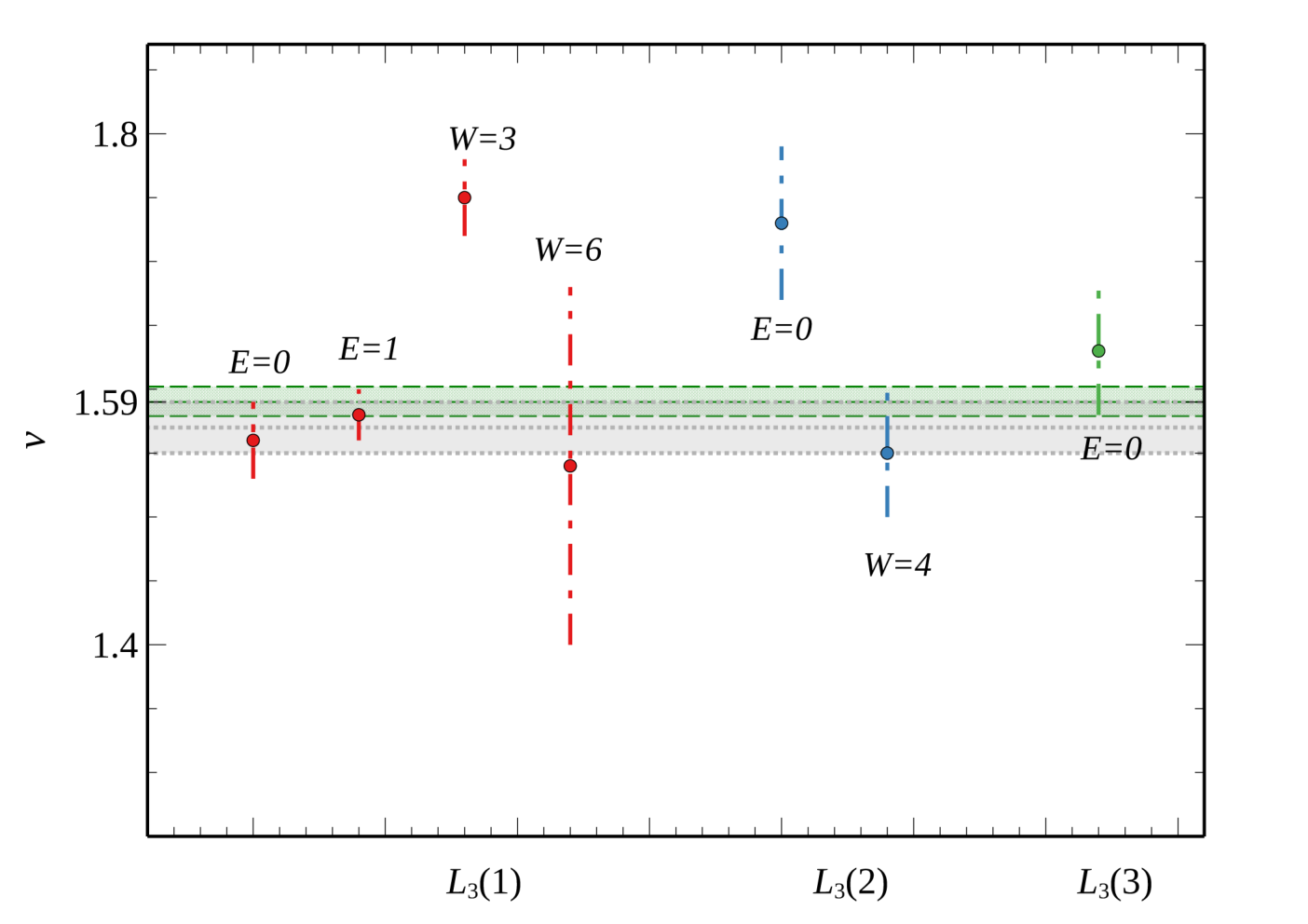
There are two ways to understand the Lieb lattices as originating from the normal simple cubic lattices: (i) as shown in Fig. 1, one can view the lattices as a cubic lattice with additionally added sites between the vertices of the cube, effectively allowing for additional back-scattering and interference along the original site-to-site connections and hence potentially leading to more localization. On the other hand, one might argue that (ii) the lattices can be constructed by deleting sites from a cubic lattice, for example a central site in Fig. 1(a) and the 6 face-centered sites. In this view, the decrease of possible transport channels should give rise to stronger effective localization. Both constructions lead to the same predictions and agree with what we find here, namely, the localization properties in all lattices show an increased localization with respect to the cubic Anderson lattice and become stronger when increases. This is, for example, clear from looking at the behaviour of in Table 1. It is instructive to study the behaviour as . From Fig. 2, we see that the overall band width decreases as increases. At the same time, the number of flat bands increases and the extremal energy of these bands extends as well towards . Hence for very large , where is simply a renormalized lattice, but renormalized sites apart, with proliferating flat bands. Our results for the critical exponent then suggest that as increases and the dispersive bands become smaller, the critical properties in each band still retain the universality of the 3D Anderson transition — at least up to that we have been able to compute (cp. Fig. 7. This is in good agreement with previous results in loosely coupled planes of Anderson models in which the universal 3D behaviour was also retained Milde2000CriticalSystems. However, for loosely coupled planes, the MIT was retained even for small interplane coupling — a truly 2D localization behavior only emerged when the interplace coupling was zero. The point of view of this work is different, i.e. the change from 3D dispersive bands with an MIT to a solely 1D system without MIT is not a continuous change, but rather an eventual replacement and shrinking of dispersive bands by a proliferation of flat bands as grows.
Acknowledgments
We wish to acknowledge the National Natural Science Foundation of China (Grant No. 11874316), the Program for Changjiang Scholars and Innovative Research Team in University (Grant No. IRT13093), and the Furong Scholar Program of Hunan Provincial Government (R.A.R.) for financial support. This work also received funding by the CY Initiative of Excellence (grant ”Investissements d’Avenir” ANR-16-IDEX-0008) and developed during R.A.R.’s stay at the CY Advanced Studies, whose support is gratefully acknowledged. We thank Warwick’s Scientific Computing Research Technology Platform for computing time and support. UK research data statement: Data accompanying this publication are available from the corresponding authors.
Appendix A Dispersions
For completeness, we here include the dispersion relations shown in Fig. 2. For , we have
| (10a) | |||||
| (10b) | |||||
where , and . For , we find
| (11a) | ||||
| (11b) | ||||
Last, for , the four doubly degenerate flat bands are given as
| (12a) | |||
| and the remaining five dispersive bands are the solutions of the th order equation | |||
| (12b) | |||
References
- (1) D. Leykam and S. Flach, APL Photonics 3, 070901 (2018).
- (2) H. Tasaki, Progress of Theoretical Physics 99, 489 (1998).
- (3) S. Miyahara, S. Kusuta, and N. Furukawa, Physica C: Superconductivity 460-462, 1145 (2007).
- (4) D. L. Bergman, C. Wu, and L. Balents, Physical Review B - Condensed Matter and Materials Physics 78, (2008).
- (5) C. Wu, D. Bergman, L. Balents, and S. Das Sarma, Physical Review Letters 99, 070401 (2007).
- (6) D. Leykam, J. D. Bodyfelt, A. S. Desyatnikov, and S. Flach, The European Physical Journal B 90, 1 (2017).
- (7) A. Julku et al., Physical Review Letters 117, 045303 (2016).
- (8) R. A. Vicencio et al., Physical Review Letters 114, 245503 (2015).
- (9) S. Mukherjee et al., Physical Review Letters 114, 245504 (2015).
- (10) D. Guzmán-Silva et al., New Journal of Physics 16, (2014).
- (11) F. Diebel et al., Physical Review Letters 116, (2016).
- (12) F. Baboux et al., Physical Review Letters 116, (2016).
- (13) S. Taie et al., Science Advances 1, (2015).
- (14) R. Shen, L. B. Shao, B. Wang, and D. Y. Xing, Physical Review B 81, 041410 (2010).
- (15) M. R. Slot et al., Nature Physics 13, 672 (2017).
- (16) P. Shukla, Physical Review B 98, 184202 (2018).
- (17) A. Ramachandran, A. Andreanov, and S. Flach, Physical Review B 96, 1 (2017).
- (18) M. Goda, S. Nishino, and H. Matsuda, Physical Review Letters 96, (2006).
- (19) W.-X. Qiu et al., Physical Review B 94, 241409 (2016).
- (20) R. Chen, D.-H. Xu, and B. Zhou, Physical Review B 96, 205304 (2017).
- (21) M. Niţǎ, B. Ostahie, and A. Aldea, Physical Review B - Condensed Matter and Materials Physics 87, 1 (2013).
- (22) M. Sun, I. G. Savenko, S. Flach, and Y. G. Rubo, Physical Review B 98, 161204 (2018).
- (23) A. Bhattacharya and B. Pal, Physical Review B 100, 235145 (2019).
- (24) E. H. Lieb, Physical Review Letters 62, 1201 (1989).
- (25) A. Mielke and H. Tasaki, Communications in Mathematical Physics 158, 341 (1993).
- (26) C.-C. Lee, A. Fleurence, Y. Yamada-Takamura, and T. Ozaki, Physical Review B 100, 045150 (2019).
- (27) X. Mao, J. Liu, J. Zhong, and R. A. Römer, 1 (2020).
- (28) P. Shukla, Physical Review B 98, 1 (2018).
- (29) B. Kramer and A. MacKinnon, Reports on Progress in Physics 56, 1469 (1993).
- (30) A. MacKinnon and B. Kramer, Physical Review Letters 47, 1546 (1981).
- (31) A. Rodriguez, L. J. Vasquez, K. Slevin, and R. A. Römer, Physical Review B 84, 134209 (2011).
- (32) K. Slevin and T. Ohtsuki, Physical Review Letters 82, 382 (1999).
- (33) Strictly speaking, the labels A and D are not needed to label , but we retain them here for the readers convenience.
- (34) V. Oseledets, Trans. Moscow Math. Soc. 19, 179 (1968).
- (35) K. Ishii, Progress of Theoretical Physics Supplement 53, 77 (1973).
- (36) C. W. Beenakker, Random-matrix theory of quantum transport, 1997.
- (37) A. Eilmes, A. M. Fischer, and R. A. Römer, Physical Review B 77, 245117 (2008).
- (38) A. MacKinnon and B. Kramer, Zeitschrift für Physik B Condensed Matter 53, 1 (1983).
- (39) P. Cain, R. A. Roemer, and M. Schreiber, Ann. Phys. 8, 507 (1999).
- (40) F. Milde, R. Römer, M. Schreiber, and V. Uski, The European Physical Journal B 15, 685 (2000).