Active and inactive quarantine in epidemic spreading on adaptive activity-driven networks
Abstract
We consider an epidemic process on adaptive activity-driven temporal networks, with adaptive behaviour modelled as a change in activity and attractiveness due to infection. By using a mean-field approach, we derive an analytical estimate of the epidemic threshold for SIS and SIR epidemic models for a general adaptive strategy, which strongly depends on the correlations between activity and attractiveness in the susceptible and infected states. We focus on strong social distancing, implementing two types of quarantine inspired by recent real case studies: an active quarantine, in which the population compensates the loss of links rewiring the ineffective connections towards non-quarantining nodes, and an inactive quarantine, in which the links with quarantined nodes are not rewired. Both strategies feature the same epidemic threshold but they strongly differ in the dynamics of active phase. We show that the active quarantine is extremely less effective in reducing the impact of the epidemic in the active phase compared to the inactive one, and that in SIR model a late adoption of measures requires inactive quarantine to reach containment.
Introduction. Understanding the effects of changes in the behaviour of individuals during epidemics is essential to improve response strategies and to foster containment Pastor-Satorras et al. 2015; Fraser et al. 2004; Hollingsworth et al. 2011; Anderson et al. 2020; Masuda and Holme 2013. This problem is nowadays particularly relevant, due to the extraordinary measures, massively introduced to limit recent disease spreading World Health Organization 2020a; World Health Organization 2020b; Gazzetta Ufficiale della Repubblica Italiana 2020; World Health Organization 2020c. In the presence of epidemics, people adapt their behaviour, modifying their actions in several ways. Infected individuals partially or totally reduce their activity, due to the appearance of symptoms or, if they are asymptomatic, due to limitations. Analogously, infected individuals can experience a reduction in their attractiveness, due to the self-protective behaviour of other individuals, who try to avoid contacts with the infected ones. All these adaptive behaviours lead to a change in activity, which can be realized in different ways, due to the peculiar structure of the society or to the perception of severity. As an example, as seen in recent real case studies Anderson et al. 2020; Horowitz and Bubola 2020, depending on the possibility to implement strong containment measures, limitation of activity in a population can be implemented in an active or inactive way. In the former, individuals avoid contacts with infected nodes, but they can readdress their activity towards non infected individuals, only shifting their focus. In the latter, individuals really become less active, in the sense that if a link is to be established with an infected node, the individual decide not to take the action, therefore reducing the overall activity of the system. A modelling framework of these effects could help in quantifying the relevance of quarantine measures Gross et al. 2006; Lagorio et al. 2011, and to assess how important is the rapidity of adoption of adaptive measures to reach containment. Simplified models, amenable to analytic control but still including the relevant dynamics, can be of some help here, as they allow testing the relevant parameters best-affecting disease containment. The natural framework to model epidemics is that of temporal networks, where links between nodes evolve in time on the same time scale of the dynamical process Pastor-Satorras et al. 2015; Holme and Saramäki 2013; Valdano et al. 2018; Holme and Liljeros 2014; Perra et al. 2012; Liu et al. 2014; Hu et al. 2018; Rizzo et al. 2014; Moinet et al. 2018; Starnini and Pastor-Satorras 2013; Masuda and Holme 2013.
We focus here on the susceptible-infected-susceptible (SIS) and susceptible-infected-recovered (SIR) models on activity-driven networks Perra et al. 2012; Starnini and Pastor-Satorras 2013; Ubaldi et al. 2016; Ubaldi et al. 2017; Burioni et al. 2017; Tizzani et al. 2018; Mancastroppa et al. 2019; Kim et al. 2018 with adaptive behaviour Funk et al. 2010; Fenichel et al. 2011. In activity-driven networks, the propensity to engage an interaction is modelled by assigning to each node an activity potential, measuring the typical number of activations (link formations) per time performed by the agent, plus an attractiveness, describing how likely it is for a node to be contacted by others Pozzana et al. 2017. The adaptive behaviour results in a change in activity and attractiveness due to infection, expressed through a general distribution function for activity and attractiveness in infected and susceptible nodes. By using an activity-attractiveness based mean-field approach, we derive an analytical estimate of the epidemic threshold for SIS and SIR epidemic models, holding for all active and inactive adaptive strategies. We also obtain analytically the epidemic prevalence of the SIS process (endemic state), while for the SIR active phase we perform numerical simulations. Interestingly, the threshold strongly depends on the correlations between the activities and attractivenesses in the susceptible and infected states. In particular, we focus on active and inactive quarantine, showing that the two containment measures have the same epidemic threshold, but they strongly differ in the dynamic of the active phase. As a result, the active quarantine is extremely less effective in reducing the impact of the epidemics compared to the inactive one, near to the epidemic threshold. We also uncover the strong effects of early adoption of quarantine measures. We show that early adoption can potentially allow to contain the epidemics with an active quarantine, without affecting the activity of the healthy, while a late adoption requires a strong reduction of the overall activity to reach an effective containment.
The model. We consider the SIS model on adaptive activity-driven networks Perra et al. 2012; Ubaldi et al. 2016; Pozzana et al. 2017: each node can be susceptible () or infected () and it is characterized by two activity parameters and two attractiveness parameters drawn form the joint distribution . Node activations occur with a Poisson process, with activation rate or , according to the node’s status. Initially all nodes are disconnected and when a node activates it creates links with randomly selected nodes (hereafter we set ): the probability to contact a node with attractiveness (with ) is given by , where is a normalization factor and depends on the adaptive behaviour as we will discuss. All links are deleted after a time step and the procedure is iterated. If a link connects an infected and a susceptible node, a contagion occurs with probability : , otherwise nothing happens. Infected nodes recover with rate , through a Poissonian process: . We call the probability that a node with activities and attractivenesses is infected at time .
The adaptive behaviour can be modelled in two ways, which we will call active and inactive. In the active case, an active node connects for sure with one of the other nodes. In this case, the normalization factor is the average attractiveness of the system at time : where we define . evolves in time according to the following equation:
| (1) |
In the inactive case, an active node may not connect to any of the nodes due to the reduction of the average attractiveness of the system caused by the infection process. In this case, at each time we set i.e. the average attractiveness when all sites are susceptible. The probability for an active node not to connect is: and the evolution of is given by:
| (2) |
Eq.s (1,2) are exact due to the mean-field nature of the model, since local correlations are destroyed at each time step and since we do not consider memory Tizzani et al. 2018; Kim et al. 2018 or burstiness effects Mancastroppa et al. 2019; Ubaldi et al. 2017; Burioni et al. 2017.
The SIS model features a phase transition between an absorbing and an active phase: the control parameter is the effective infection rate (in literature the threshold is sometimes discussed in terms of the adimensional parameter ). Through a linear stability analysis, we obtain the epidemic threshold , which remarkably is the same for the active and inactive adaptive behaviour supplemental:
| (3) |
From Eq. (3), we see that is reduced in the presence of strong correlations between susceptible and infected states. In particular, this means that epidemic spreading is favoured by the presence of nodes which keep their high activity and/or high attractiveness both when they are susceptible and when they are infected (super-spreaders). Eq. (3) also reproduces the non-adaptive case without attractiveness Perra et al. 2012 (fixing and ) and the non-adaptive case with attractiveness (NAdwA) Pozzana et al. 2017 (fixing and ) . If ( arbitrary constant), as observed in real systems Pozzana et al. 2017, we obtain .
From Eq.s (1,2), the stationary infection probability in the active (Eq. (4)) and inactive (Eq. (5)) cases is:
| (4) |
| (5) |
Contrarily to the epidemic threshold, the active phase depends on the implementation of the adaptive behaviour. This suggests that it is not enough to investigate the epidemic threshold, or the basic reproductive number : the same population with two different dynamics feature a different epidemic active phase.
The proposed model allows studying several adaptive behaviours; in particular by setting the functional form of one can model a mild social distancing, like the sick-leave practice where only activity is reduced in infected nodes Ariza et al. 2018; a targeted adaptive prescription where and vary only for some activity classes, more exposed to risk Anderson et al. 2020; Mossong et al. 2008; moreover one can consider different distributions of and modelling different social systems Pozzana et al. 2017; Perra et al. 2012. Here we will focus on a strong social distancing approach like quarantine.
Active and inactive quarantine. Nowadays the effects of quarantine on epidemic spreading are of enormous interest due to the extraordinary isolation measures to limit the spread of COVID-19 taken by several countries World Health Organization 2020a; World Health Organization 2020b; World Health Organization 2020c; Gazzetta Ufficiale della Repubblica Italiana 2020. In our model we consider that a fraction of the nodes, when infected, goes to quarantine by setting both and to zero. Indeed, we expect that a fraction of the infected nodes does not perform quarantine since they may not be aware of the infection (no symptoms) or they do not follow the prescriptions of social distancing: thus takes into account the uncertainty in the application of the containment measures.
Our approach naturally distinguishes an active quarantine from an inactive one. In the active quarantine an active node selects randomly its contact among the non-quarantining nodes: links directed to quarantining nodes are effectively rewired towards potentially susceptible or non-quarantining infected nodes. Dynamical link rewiring can produce non-trivial effects on epidemic spreading, as observed in Gross et al. 2006 for static networks. Indeed, rewiring induces new connections among not-quarantining nodes and this can strengthen the epidemics Scarpino et al. 2016; Gross et al. 2006. On the contrary, in the inactive case the population does not compensate the ineffective links towards nodes in quarantine and the effective contagion is reduced.
We consider a system with a linear correlation , accordingly to observations on real data Pozzana et al. 2017. Very active hubs, generating many links, are also very attractive, receiving just as many. If a fraction of the population performs quarantine (), while the remaining keeps and , we get , where is the Dirac-delta function. The epidemic threshold is:
| (6) |
The quarantine increases the epidemic threshold of the non adaptive case by a factor which is particularly significant when .
Although the active and inactive quarantine display the same epidemic threshold, the active phase is different. The stationary infection probability in the active quarantine is:
| (7) |
while, in the inactive case it is:
| (8) |

Eq.s (7,8) can be solved self consistently fixing : we consider a power-law distribution with Perra et al. 2012; Ubaldi et al. 2016, modelling the presence of heterogeneities and large activity fluctuations. Indeed, many real human systems feature a broad power-law distribution of with exponent Ubaldi et al. 2016; Perra et al. 2012; Karsai et al. 2014. Heterogeneities account for different social propensity in engaging social interactions (e.g. different works, social roles), producing different number of contacts over time Perra et al. 2012; Ubaldi et al. 2016: in the following we will fix .
In Fig. 1(a) we plot the ratio between epidemic prevalence and the prevalence in the NAdwA case (i.e. at ) as a function of ; quarantine measures induce an effective reduction of the final prevalence (of a factor ) only for .
This is confirmed by Fig. 1(b) where we plot the prevalence as a function of for and , so here we set in the range , consistently with the recent implementations of extended quarantine World Health
Organization 2020c; Gazzetta Ufficiale della Repubblica
Italiana 2020.
Interestingly, Figures 1(a-b) show that the epidemic prevalence of the inactive quarantine is much smaller compared to the active one, making the latter strategy extremely less effective.
In this respect, in Fig. 1(c) we plot the ratio between the epidemic prevalence of the active and inactive case as a function of . The difference is maximized when (depending on ) and it increases with higher values. Also for more realistic values, where the quarantine is effective in moving the systems near to the critical point, in active quarantine the epidemic prevalence is about twice that of the inactive one.
Effects of quarantine on SIR epidemic model. In the SIR model, a recovered node is no more susceptible but enters at the recovery rate into the immune state where it cannot be infected: . We consider the SIR model on our activity-driven model: each node is described by six parameters extracted from the joint distribution . Hereafter, we consider the case in which all recovered nodes behave as if they were susceptible and : , with equal to the previous distribution for quarantine.
Due to the mean-field nature of the model, the epidemic threshold is the same of the SIS model independently of and and it is equal for active and inactive quarantine (Eq. 6). On the contrary, the dynamics in the active phase is known to be different. In particular, the SIR model lacks an endemic steady state, since the dynamics always halts reaching a state in which no infected nodes are present. The final fraction of recovered nodes is used as an order parameter. However the stationary condition on the dynamical equation does not provide a solution for and numerical simulation are necessary to obtain insight on the dynamics.
We implement the SIR model with a continuous time Gillespie-like algorithm Gillespie 1976; supplemental, in a system of nodes and we average over a number of realizations of the dynamical evolution and of the disorder, so that the error on is lower than 1%. The initial conditions are imposed infecting the node with the highest activity Boguñá et al. 2013, immediately implementing the quarantine measures.
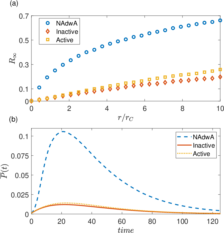
In Fig. 2(a) we compare of the NAdwA case with the active/inactive quarantines, computed as a function of , fixing the same . Both quarantines deeply lowers the epidemic final-size compared to the non-adaptive case, however the active quarantine produces an higher than the inactive one. The epidemic final-size of the active case is about 10% higher than the inactive one for small infectivity , i.e. the significant regime for an effective quarantine. Both quarantine strategies greatly impact on the SIR dynamics: Fig. 2(b) shows the temporal evolution of the average infection probability for and . The infection peak is strongly flattened and occurs slightly before, compared to the NAdwA dynamics. This is expected, as social distancing anticipates the decay of the fraction of infected nodes. The height of the peak for the active quarantine is 10%-20% larger than the inactive one for (depending on value). These estimates outlines a difference between the two strategies even if the effect is smaller compared to the SIS model.
Thus far we considered quarantine measures implemented at the beginning of the epidemic. However typically the containment measures are applied only after a fraction of the population has been infected. This is relevant for the SIR model, since the dynamics and depend strongly on the initial conditions, contrary to the SIS. Therefore, we let the epidemic process evolve on the NAdwA network, without adaptive behaviours, until a fraction of the population has been infected. Then, quarantine measures are implemented and are kept effective until the end of the epidemic.


In Fig. 3 we plot as a function of , fixing and : both strategies show the importance of an early adoption of quarantine, since increases significantly with , despite in a different way for the two strategies. In the inactive quarantine approximatively we get , i.e. the epidemic final-size for the quarantine at is summed to the fraction of infected nodes before the quarantine adoption. On the contrary, in active quarantine, grows very rapidly with and the difference between the two strategies in weakening the epidemic becomes very different. In the insert of Fig. 3, we show the fast growth with of the ratio between the epidemic final-size of the active and inactive case. If the quarantine is implemented immediately (), the difference is about 10%; if the containment measures are applied when about 2% of the population has been infected for the active case can be up to times the inactive one (for ).
Finally, we investigate the effects of the timing in the quarantine adoption on the SIR temporal dynamics: in Fig. 4(a)-(b) we plot the infection peak respectively for and , fixing and . If the fraction increases, both quarantines are extremely less effective in flattening the infection peak, showing the importance of early adoption of measures. Comparing these results with Fig. 2(b) (), for the inactive infection peak is significantly flattened compared to the active one. This is highlighted in Fig. 4(c) where we plot the ratio between the height of the infection peak in the active and inactive case. If the containment measures are applied immediately, the difference is about 10%; if they are applied when a small fraction between 0.25% and 4% of the population has been infected, the active peak is about twice larger than the inactive one at ; a smaller but significant difference is observed also for .
Our results hold for a realistically heterogeneous population Perra et al. 2012 with extensive containment measures, such as those recently implemented World Health Organization 2020c; Gazzetta Ufficiale della Repubblica Italiana 2020, able to move the system just above the threshold (). In particular, in this range of parameters, our findings support the crucial role of timing in the adoption of containment measures. If the measures are implemented immediately, both active and inactive strategies are effective in reducing the infection peak of 75%-85% (depending on ) compared to the NAdwA case. However, any delay in the adoption of quarantine measures produces a drastic reduction in the effectiveness of the strategies. More interestingly, the differences between the two strategies increases in the case of a late adoption. This means that if containment measures are not immediately taken, a stringent inactive quarantine, also binding the healthy to decrease their activity, is required to produce an effective result. With an early adoption, of course an inactive quarantine is still the best choice, but if this strong social distancing cannot be implemented for social reasons, a strategy focusing only on infected individuals is also able to produce a containment. Such effective results in both cases depend on the ability to obtain a large adhesion to quarantine measures ().
References
- Pastor-Satorras et al. (2015) R. Pastor-Satorras, C. Castellano, P. Van Mieghem, and A. Vespignani, Rev. Mod. Phys. 87, 925 (2015).
- Fraser et al. (2004) C. Fraser, S. Riley, R. M. Anderson, and N. M. Ferguson, Proc. Natl. Acad. Sci. USA 101, 6146 (2004).
- Hollingsworth et al. (2011) T. D. Hollingsworth, D. Klinkenberg, H. Heesterbeek, and R. M. Anderson, PLOS Comput. Biol. 7, 1 (2011).
- Anderson et al. (2020) R. M. Anderson, H. Heesterbeek, D. Klinkenberg, and T. D. Hollingsworth, The Lancet 395, 931 (2020).
- Masuda and Holme (2013) N. Masuda and P. Holme, F1000Prime Rep. 5, 6 (2013).
- World Health Organization (2020a) World Health Organization, “Statement on the meeting of the international health regulations (2005) emergency committee regarding the outbreak of novel coronavirus (2019-ncov),” (2020a).
- World Health Organization (2020b) World Health Organization, “Coronavirus disease (covid-2019) situation reports - 62,” (2020b).
- Gazzetta Ufficiale della Repubblica Italiana (2020) Gazzetta Ufficiale della Repubblica Italiana, “Further implementing provisions of the d.l. 6/2020, containing urgent measures regarding the containment and management of the epidemiological emergency of covid-19, applicable on the whole italian national territory,” (2020).
- World Health Organization (2020c) World Health Organization, “Report of the who-china joint mission on coronavirus disease 2019 (covid-19),” (2020c).
- Horowitz and Bubola (2020) J. Horowitz and E. Bubola, New York Times (28th february 2020).
- Gross et al. (2006) T. Gross, C. J. D. D’Lima, and B. Blasius, Phys. Rev. Lett. 96, 208701 (2006).
- Lagorio et al. (2011) C. Lagorio, M. Dickison, F. Vazquez, L. A. Braunstein, P. A. Macri, M. V. Migueles, S. Havlin, and H. E. Stanley, Phys. Rev. E 83, 026102 (2011).
- Holme and Saramäki (2013) P. Holme and J. Saramäki, Temporal Networks (Springer, 2013).
- Valdano et al. (2018) E. Valdano, M. R. Fiorentin, C. Poletto, and V. Colizza, Phys. Rev. Lett. 120, 068302 (2018).
- Holme and Liljeros (2014) P. Holme and F. Liljeros, Sci. Rep. 4, 4999 (2014).
- Perra et al. (2012) N. Perra, B. Gonçalves, R. Pastor-Satorras, and A. Vespignani, Sci. Rep. 2, 469 (2012).
- Liu et al. (2014) S. Liu, N. Perra, M. Karsai, and A. Vespignani, Phys. Rev. Lett. 112, 118702 (2014).
- Hu et al. (2018) P. Hu, L. Ding, and X. An, Phys. Rev. E 98, 062322 (2018).
- Rizzo et al. (2014) A. Rizzo, M. Frasca, and M. Porfiri, Phys. Rev. E 90, 042801 (2014).
- Moinet et al. (2018) A. Moinet, R. Pastor-Satorras, and A. Barrat, Phys. Rev. E 97, 012313 (2018).
- Starnini and Pastor-Satorras (2013) M. Starnini and R. Pastor-Satorras, Phys. Rev. E 87, 062807 (2013).
- Ubaldi et al. (2016) E. Ubaldi, N. Perra, M. Karsai, A. Vezzani, R. Burioni, and A. Vespignani, Sci. Rep. 6, 35724 (2016).
- Ubaldi et al. (2017) E. Ubaldi, A. Vezzani, M. Karsai, N. Perra, and R. Burioni, Sci. Rep. 7, 46225 (2017).
- Burioni et al. (2017) R. Burioni, E. Ubaldi, and A. Vezzani, J. Stat. Mech.: Theory Exp. 2017, 054001 (2017).
- Tizzani et al. (2018) M. Tizzani, S. Lenti, E. Ubaldi, A. Vezzani, C. Castellano, and R. Burioni, Phys. Rev. E 98, 062315 (2018).
- Mancastroppa et al. (2019) M. Mancastroppa, A. Vezzani, M. A. Muñoz, and R. Burioni, J. Stat. Mech.: Theory Exp. 2019, 053502 (2019).
- Kim et al. (2018) H. Kim, M. Ha, and H. Jeong, Phys. Rev. E 97, 062148 (2018).
- Funk et al. (2010) S. Funk, M. Salathé, and V. A. A. Jansen, J. R. Soc. Interface 7, 1247 (2010).
- Fenichel et al. (2011) E. P. Fenichel, C. Castillo-Chavez, M. G. Ceddia, G. Chowell, P. A. G. Parra, G. J. Hickling, G. Holloway, R. Horan, B. Morin, C. Perrings, M. Springborn, L. Velazquez, and C. Villalobos, Proc. Natl. Acad. Sci. USA 108, 6306 (2011).
- Pozzana et al. (2017) I. Pozzana, K. Sun, and N. Perra, Phys. Rev. E 96, 042310 (2017).
- (31) See Supplemental Material for the analytical derivation of the epidemic threshold for the SIS model on the proposed adaptive network, and for a sketch of the Gillespie-like algorithm performed to simulate the SIR dynamics.
- Ariza et al. (2018) M. Ariza, C. Guerrisi, C. Souty, L. Rossignol, C. Turbelin, T. Hanslik, V. Colizza, and T. Blanchon, BJGP Open 1 (2018).
- Mossong et al. (2008) J. Mossong, N. Hens, M. Jit, P. Beutels, K. Auranen, R. Mikolajczyk, M. Massari, S. Salmaso, G. S. Tomba, J. Wallinga, J. Heijne, M. Sadkowska-Todys, M. Rosinska, and W. J. Edmunds, PLOS Med. 5, 1 (2008).
- Scarpino et al. (2016) S. V. Scarpino, A. Allard, and L. Hébert-Dufresne, Nat. Phys. 12, 1042 (2016).
- Karsai et al. (2014) M. Karsai, N. Perra, and A. Vespignani, Sci. Rep. 4, 4001 (2014).
- Gillespie (1976) D. T. Gillespie, J. Comput. Phys. 22, 403 (1976).
- Boguñá et al. (2013) M. Boguñá, C. Castellano, and R. Pastor-Satorras, Phys. Rev. Lett. 111, 068701 (2013).