∎

Optimal Control of Aquatic Diseases: A Case Study of Yemen’s Cholera OutbreakJournal: JOTADedication: Communicated by Alberto d’Onofrio

Ana P. Lemos-Paião Affiliation: Center for Research and Development in Mathematics and Applications (CIDMA),
Department of Mathematics, University of Aveiro, 3810-193 Aveiro, Portugal
anapaiao@ua.pt Cristiana J. Silva
Delfim F. M. Torres Ezio Venturino Affiliation: Department of Mathematics “Giuseppe Peano”,
Università di Torino, via Carlo Alberto 10, 10123, Torino, Italy
Member of the INdAM research group GNCS
ezio.venturino@unito.it

Received: April 6, 2019; Revised: October 12, 2019 and January 21, 2020; Accepted: April 15, 2020

Abstract

We propose a mathematical model for the transmission dynamics of some strains of the bacterium Vibrio cholerae, responsible for the cholera disease in humans. We prove that, when the basic reproduction number is equal to one, a transcritical bifurcation occurs for which the endemic equilibrium emanates from the disease-free point. A control function is introduced into the model, representing the distribution of chlorine water tablets for water purification. An optimal control problem is then proposed and analyzed, where the goal is to determine the fraction of susceptible individuals who should have access to chlorine water tablets in order to minimize the total number of new infections plus the total cost associated with the distribution of chlorine water tablets, over the considered period of time. Finally, we consider real data of the cholera outbreak in Yemen, from 27 April 2017 to 15 April 2018, choosing the values of the parameters of the uncontrolled model that fit the real data. Using our optimal control results, we show, numerically, that the distribution of chlorine water tablets could have stopped, in a fast way, the worst cholera outbreak that ever occurred in human history. Due to the critical situation of Yemen, we also simulate the case where only a small percentage of susceptible individuals has access to chlorine water tablets and obtain an optimal control solution that decreases, substantially, the maximum number of infective individuals attained at the outbreak.

Keywords:

SIQRB cholera model Equilibrium points Feasibility and local stability Optimal control 2018 cholera outbreak in Yemen

MSC

34C60 49K15 92D30

1 Introduction

Cholera is an acute diarrhoeal illness caused by infection of the intestine with some strains of the bacterium Vibrio cholerae, which lives in an aquatic medium. Cholera remains a global threat to public health and an indicator of inequity and lack of social development WHO_cholera; LPST. Cholera is a disease of poverty and closely linked to poor sanitation and a lack of clean drinking water WHO:cholera:vaccines. The ingestion of contaminated water can cause cholera outbreaks, as John Snow proved, in 1854 Shuai. This is a way of transmission of the disease, but other ones exist. For example, susceptible individuals can become infected if they come in contact with infectious individuals. If individuals are at an increased risk of infection, then they can transmit the disease to other persons that live with them by sharing food preparation or water storage containers Shuai. An individual can be infected with or without symptoms. Some symptoms are watery diarrhoea, vomiting, and leg cramps. If an infective individual does not have treatment, then he becomes dehydrated, suffering of acidosis and circulatory collapse. This situation can lead to death within 12 to 24 hours Mwasa; Shuai. Some studies and experiments suggest that a recovered individual can be immune to the disease during a period of 3 to 10 years. However, recent discoveries suggest that immunity can be lost after a period of weeks to months Neilan; Shuai.

Since 1979, several mathematical models for the transmission of cholera have been proposed: see, e.g., Capasso:1979; Capone; Codeco:2001; Hartley:2006; Hove-Musekwa; Joh:2009; LPST; LPaiaoSilvaTorresYemen2018; Mukandavire:2008; Mwasa; Neilan; Pascual; Shuai and references cited therein. In Neilan, the authors propose an SIR (Susceptible–Infectious–Recovered) type model and consider two classes of bacterial concentrations (hyperinfectious and less-infectious) and two classes of infective individuals (asymptomatic and symptomatic). In Shuai, another SIR-type model is proposed that incorporates hyperinfectivity (where infectivity varies with the time elapsed since the pathogen was shed) and temporary immunity, using distributed delays. The authors of Mwasa incorporate in a SIR-type model public health educational campaigns, vaccination, quarantine and treatment, as control strategies in order to curtail the disease.

The use of quarantine for controlling epidemic diseases has always been controversial, because such strategy raises political, ethical, and socioeconomic issues and requires a careful balance between public interest and individual rights Tognotti:quarantine. Quarantine was adopted as a mean of separating persons, animals, and goods, which may have been exposed to a contagious disease. Since the fourteenth century, quarantine has been the cornerstone of a coordinated disease-control strategy, including isolation, sanitary cordons, bills of health issued to ships, fumigation, disinfection, and regulation of groups of persons who were believed to be responsible for spreading the infection Matovinovic; Tognotti:quarantine. The World Health Organization (WHO) does not recommend quarantine measures and embargoes on the movement of people and goods for cholera. However, cholera is still on the list of quarantinable diseases of the EUA National Archives and Records Administration CenterDiseaseControl.

In this paper, we propose a SIQR (Susceptible–Infectious–Quarantined–Recovered) type model based on LPST, where it is assumed that infective individuals are subject to quarantine during the treatment period. We refine the model of LPST, considering the important situation related to the fact that to become infected, a healthy individual must intake bacteria from the environment and, by doing it, these bacteria are removed from the aquatic environment. The model here proposed improves the one in LPST, since the removal of the ingested bacteria from the environment by susceptible individuals was not previously considered and it must be assumed. Our aim is to discover what happens when an efficient strategy through quarantine is implemented.

The consequences of a humanitarian crisis, such as disruption of water and sanitation systems or the displacement of populations to inadequate and overcrowded camps, can increase the risk of cholera transmission WHO_cholera. The number of cholera cases reported by WHO has continued to be high over the last few years. During 2016, $132121$ cases were notified from 38 countries, including 2420 deaths WHO_cholera. Recently, in Yemen the largest outbreak of cholera in the history of the world has occurred, TelegraphNews. The epidemic began in October 2016 and in February–March 2017 was in decline. However, on 27 April 2017, the epidemic broke out again. This happened ten days after Sanaa’s sewer system had stopped working. Problems in infrastructures, health, water and sanitation systems in Yemen, allowed the fast spread of the disease wikipedia_cholera_yemen. Between 27 April 2017 and 15 April 2018, there were 1 090 280 suspected cases reported and 2 275 deaths due to cholera WHO_15abril2018. In Nishiura, this outbreak is studied mathematically, forecasting the cholera epidemic in Yemen and explicitly addressing the reporting delay and ascertainment bias. On the other hand, in LPaiaoSilvaTorresYemen2018 a SIQRV (Susceptible–Infectious–Quarantined–Recovered–Vaccinated) type model is proposed, considering vaccination of susceptible individuals and describing well the cholera outbreak in Yemen, between 27 April 2017 and 15 April 2018. In Sardar, a compartmental model with periodic environment is proposed, using a real-life data set of cholera epidemic for Zimbabwe, between 2008 and 2011.

Optimal control is a branch of mathematics developed to find optimal ways to control a dynamical system Cesari_1983; Fleming_Rishel_1975; Pontryagin_et_all_1962. There are few papers that apply optimal control to cholera models, see e.g. Neilan; LPST; Sardar. Here we propose and analyze one such optimal control problem, where the control function represents the fraction of susceptible individuals $S$ who has access to chlorine water tablets (CWT) for water purification. Therefore, they are protected from infection. The objective is to find the optimal strategy through the use of CWT that minimizes the total number of new infections plus the total cost associated with CWT interventions. CWT are effervescent tablets that kill micro-organisms in water to prevent cholera, typhoid, dysentery, and other water borne diseases. There are different sizes of CWT and each tablet size is formulated to treat a specific volume of water, ranging from 1 liter to 2 500 liters.

We prove that the extremal controls, derived from the Pontryagin Maximum Principle, satisfy the so-called strict bang-bang property Osmolovskii. Through numerical simulations, we show that the strategy given by the solution of the optimal control problem could have stopped, in a short time, the cholera outbreak on Yemen. Moreover, we simulate the cases of low, sufficient, and abundant resources, finding the interval of time needed to stop the outbreak in Yemen.

The paper is organized as follows. In Section 2, we propose a model for cholera transmission dynamics. We analyze, in Section 3, the positivity and boundedness of the solutions, as well as the local stability and feasibility of the disease-free and endemic equilibria. In Section 4, we propose and analyze an optimal control problem for the minimization of the number of new infections through the distribution of CWT. Section 5 is devoted to numerical simulations and a case study in Yemen. The concluding Section 6 discusses the optimal impact of CWT distribution on the control of the cholera outbreak in Yemen, pointing also some directions for future work.

2 Model Setup

The model contains the fundamental populations, identified as follows. The humans are subdivided into the susceptible $S$ , infective $I$ , quarantined $Q$ , and recovered $R$ . Then we also consider the free bacteria population living in the environment, $B$ . This is an important specification, as to become infected, a healthy individual must intake bacteria from the environment and, in doing so, these bacteria are removed from the aquatic medium. This feature, absent in LPST, must be incorporated in the model, to have a meaningful formulation. The model equations read as follows:

\begin{cases}\begin{split}\dot{S}(t)=\ &\Lambda-\displaystyle\frac{\beta B(t)S(t)}{\kappa+B(t)}+\omega R(t)-\mu S(t)=:f_{1},\\[8.5359pt] \dot{I}(t)=\ &\displaystyle\frac{\beta B(t)S(t)}{\kappa+B(t)}-(\delta+\alpha_{1}+\mu)I(t)=:f_{2},\\[8.5359pt] \dot{Q}(t)=\ &\delta I(t)-(\varepsilon+\alpha_{2}+\mu)Q(t)=:f_{3},\\[8.5359pt] \dot{R}(t)=\ &\varepsilon Q(t)-(\omega+\mu)R(t)=:f_{4},\\[8.5359pt] \dot{B}(t)=\ &\eta I(t)-dB(t)-\displaystyle\frac{\rho B(t)S(t)}{\kappa+B(t)}=:f_{5}.\end{split}\end{cases}

(1)

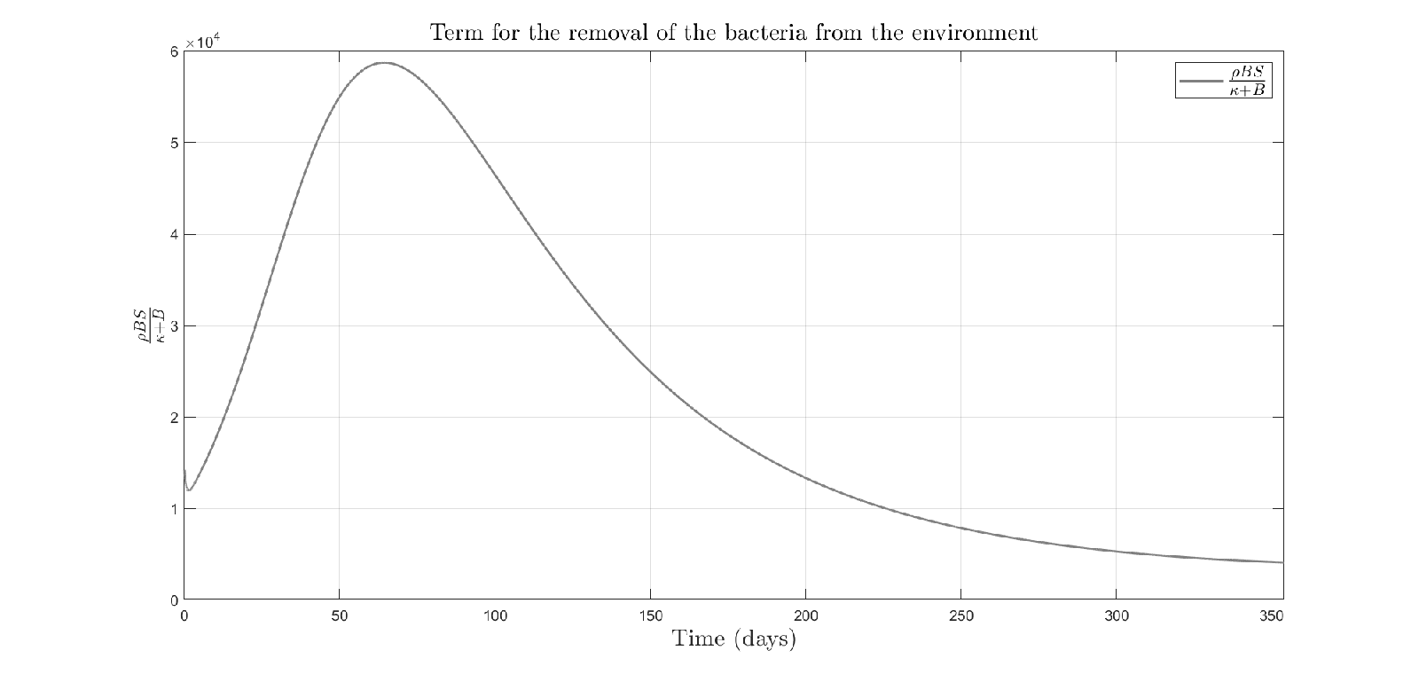
It should be noted that the new term for the removal of bacteria from the environment, through their uptake by susceptible individuals, here added with respect to LPST, is very relevant. Using the values for the parameters of Section 5, Figure 1 quantifies the new term for the removal of bacteria from the environment along time. As it can be seen in this figure, the new term is quantitatively important.

Refer to caption — Figure 1: New term for the removal of bacteria from the environment through their uptake by susceptible individuals.

We could also consider that infected individuals also ingest contaminated water. This would account for the modification of the last/bacteria equation, by including additional terms $-aBI/(\kappa+B)$ and $-bBR/(\kappa+B)$ . However, we verified that these new terms are not quantitatively important.

The first equation describes the evolution of the healthy people. We assume to have an input of new individuals at constant rate $\Lambda$ , that can get infected by ingestion of bacteria from the environment. This mechanism is expressed by the second term, with a saturating response function in terms of the bacteria. It behaves linearly at first, as the more bacteria are acquired, the higher the probability of getting the infection. But this holds up to a certain point, because if the water already ingested is full of germs, to drink more of it, will not substantially increase the threat to the health of the consumer, which is already quite endangered. Therefore, the infection contagion level will saturate at rate $\beta$ . Note that more bacteria to be ingested to start the infection is already embedded in this parameter. The remaining terms in the equation represent the individuals that, after recovery, become susceptible again, at rate $\omega$ , and the natural human mortality, at rate $\mu$ .

The second equation for the infective contains the new recruitments, coming from the healthy individuals as described above, and then the losses of this class, namely, the migration to the quarantined class, at rate $\delta$ , the disease-related mortality, at rate $\alpha_{1}$ , and the natural mortality, at rate $\mu$ . Although the assumption that all infected individuals enter the quarantine stage may be a far-fetched assumption, if such ambitious studies are not carried out, almost no one will strive to improve recent and problematic endemic realities. The uptake of viruses from bacteria in an aquatic environment is described in MR1629476 (but see also MR2492346 for a revisitation of the above model), a system that roughly corresponds to the first, second and last equation in the model at hand, where now bacteria take the place of viruses and people replace bacteria. Here, we further modify it considering that usually in ecological settings the quantity of food (or water) consumption is usually assumed to be modeled via a Holling type II response function. In turn, the mechanism describes the fact that the infection rate will saturate with the number of bacteria.

The quarantined class, third equation, incorporates the infective individuals who are so identified at rate $\delta$ . Then, it can lose people in three different ways: through migration to the recovered class, at rate $\varepsilon$ ; still by disease-related mortality, but at a possibly different rate $\alpha_{2}$ ; or, finally, by natural mortality, at rate $\mu$ .

The recovered individuals come from the quarantined class at rate $\varepsilon$ and leave either by returning susceptible at rate $\omega$ or by natural mortality. In this case, the people are not ill and, therefore, the disease-related mortality is not present.

The last equation accounts for the free bacteria in the environment, i.e., the water. In this medium they cannot survive, their mortality rate being $d$ . Nevertheless, they are continuously reversed into it by the infective individuals $I$ , at rate $\eta$ . Indeed, within the body of the infective, they do reproduce, this indeed being the cause of the illness, and are then released in the open environment. A similar phenomenon could occur for the quarantined individuals, who are still subject to the disease, but it is assumed that, as they are isolated and treated in the hospitals, measures are taken so that they cannot propagate the infection. In particular, they are prevented from fouling the water with new bacteria coming from the dejections of their bodies. The third term in the equation describes, as mentioned before stating the model, the uptake of bacteria from the water by healthy individuals during the infection process. We can easily assume that quarantined people are taken care of and therefore not exposed to and ingest contaminated water. It is also reasonable to assume that, after recovery, individuals would be very careful about the water they consume, in view of the fact that during the treatment period they would be informed about the source of the disease. We also assume that there is a prompt response of the authorities to infection through treatment (quarantine) so that the amount of bacteria ingested by infected individuals is residual and can be neglected. Therefore, we can assume that bacteria are not taken up from the environment by these classes of individuals. On the other hand, as already stated, they are essential in rendering susceptible individuals diseased.

In a more abstract setting, we can rewrite (1) by introducing the vector of the time-dependent variables,

X=(x_{1},x_{2},x_{3},x_{4},x_{5})=(S,I,Q,R,B),

(2)

for which (1), in compact form, becomes:

\dot{x_{i}}(t)=f_{i}(x_{1},\ldots,x_{5}),\quad i=1,\ldots,5.

(3)

3 Analysis of the Model

Our analysis of (1) follows the pattern used in LPST.

3.1 Preliminary Results

Assuming the ecologically meaningful nonnegative initial conditions for the populations, the solutions of the dynamical system remain nonnegative for all time. This result is contained in Lemma 1 of LPST and translates in this situation without any change. The solutions not only remain in the positive cone, but are also bounded and the positively invariant set $\Omega$ is the same already found in LPST, namely:

\begin{gathered}\Omega=\Omega_{H}\times\Omega_{B},\qquad\Omega_{B}=\left\{B\in\mathbb{R}_{0}^{+}:B(t)\leq\frac{\Lambda\eta}{\mu d}\right\},\\ \Omega_{H}=\left\{(S,I,Q,R)\in\left(\mathbb{R}_{0}^{+}\right)^{4}:S(t)+I(t)+Q(t)+R(t)\leq\frac{\Lambda}{\mu}\right\}.\end{gathered}

(4)

The proof is essentially the same, with only a change in the derivation of the upper bound for the bacteria population, which is obtained by dropping the last term of the last equation in (1) to obtain the same bound:

\dot{B}(t)\leq\eta I(t)-dB(t)\leq\eta\frac{\Lambda}{\mu}-dB(t)\,.

3.2 System’s Equilibria

The only possible equilibria of model (1) are the disease-free point (DFE) and coexistence, or the endemic equilibrium (EE), as in LPST. However, we will repeat here the analysis in some detail as it entails some relevant differences.

As for the DFE, we find again

E^{0}=(S^{0},I^{0},Q^{0},R^{0},B^{0})=\left(\frac{\Lambda}{\mu},0,0,0,0\right).

(5)

The basic reproduction number $R_{0}$ can then be evaluated, following Mwasa; Driessche.

Proposition 1

The basic reproduction number of model (1) is

R_{0}=\dfrac{\beta\Lambda\eta}{(\delta+\alpha_{1}+\mu)\,\left(\mu\kappa d+\rho\,\Lambda\right)}.

(6)

Proof

Follows easily using the methods described in Diekmann. $\Box$

The basic reproduction number proves to be instrumental in the local stability issue of the DFE $E^{0}$ , as it is shown in the next result.

Theorem 3.1

The disease-free equilibrium $E^{0}$ of model (1) is locally asymptotic stable if

R_{0}<1.

(7)

Proof

Let us write the right-hand side of system (1) as $\mathscr{F}-\mathscr{V}$ according to the approach of Driessche. The characteristic equation of (1) evaluated at the DFE, $p(\chi)=\det(F_{0}-V_{0}-\chi I_{5})$ with $F_{0}$ and $V_{0}$ the Jacobian matrices of $\mathscr{F}$ and $\mathscr{V}$ computed at the disease free equilibrium $E^{0}$ , respectively, factorizes to produce three explicit eigenvalues, $-\mu<0$ , $-a_{2}<0$ , and $-a_{3}<0$ , and a quadratic equation in $\chi$ :

(a_{1}+\chi)\left(d+\dfrac{\rho\Lambda}{\mu\kappa}+\chi\right)-\displaystyle\frac{\beta\Lambda\eta}{\mu\kappa}=0,

for which the Routh–Hurwitz conditions are easily seen to hold if

a_{1}\left(d+\dfrac{\rho\Lambda}{\mu\kappa}\right)-\displaystyle\frac{\beta\Lambda\eta}{\mu\kappa}>0,

which amounts to the condition (7). $\Box$

A converse result holds in case of the opposite condition, as illustrated in the following result.

Proposition 2

Let $a_{1}=\delta+\alpha_{1}+\mu$ , $a_{2}=\varepsilon+\alpha_{2}+\mu$ , and $a_{3}=\omega+\mu$ . Assume that $\lambda^{*},\ \delta,\ \varepsilon,\ \omega>0$ . If $R_{0}>1$ , then model (1) has the endemic equilibrium

E^{*}=(S^{*},I^{*},Q^{*},R^{*},B^{*})=\left(\frac{\Lambda a_{1}a_{2}a_{3}}{D},\frac{\Lambda a_{2}a_{3}\lambda^{*}}{D},\frac{\Lambda\delta a_{3}\lambda^{*}}{D},\frac{\Lambda\delta\varepsilon\lambda^{*}}{D},(\beta\eta-\rho a_{1})\frac{\Lambda a_{2}a_{3}\lambda^{*}}{\beta Dd}\right),

(8)

where

D=a_{1}a_{2}a_{3}(\lambda^{*}+\mu)-\delta\varepsilon\omega\lambda^{*},\quad\lambda^{*}=\beta B^{*}(\kappa+B^{*})^{-1},

(9)

which is feasible if

\beta\eta>\rho a_{1}.

(10)

Proof

For this equilibrium to be feasible, the transmission rate must be strictly positive:

\beta B^{*}(t)\left(\kappa+B^{*}(t)\right)^{-1}>0.

Solving in turn the second, third, and fourth equilibrium equation of (1), we find

S^{*}=\dfrac{a_{1}}{\lambda^{*}}I^{*},\quad I^{*}=\dfrac{a_{2}}{\delta}Q^{*},\quad Q^{*}=\dfrac{a_{3}}{\varepsilon}R^{*}.

Then, we obtain

S^{*}=\dfrac{a_{1}a_{2}a_{3}}{\lambda^{*}\delta\varepsilon}R^{*}.

Substituting the last evaluated value of $S^{*}$ into the first equilibrium equation, we then obtain $\delta\varepsilon\lambda^{*}\Lambda-DR^{*}=0$ , which gives the fourth component of (8), and by back substitution also the first three. Finally, the fifth equation provides the value of $B^{*}$ , which must be nonnegative to be feasible, giving thus (10). Now, from $\lambda^{*}=\beta B^{*}(\kappa+B^{*})^{-1}$ , substituting the value of $B^{*}$ and rearranging, we obtain

\{[\Lambda(\beta\eta-\rho a_{1})+\kappa\beta da_{1}]a_{2}a_{3}-\kappa\beta d\delta\varepsilon\omega\}\lambda^{*}=[\beta\Lambda\eta-a_{1}(\rho\Lambda+\mu\kappa d)]\beta a_{2}a_{3}.

It follows that

\lambda^{*}=\dfrac{\beta(R_{0}-1)a_{1}a_{2}a_{3}(\rho\Lambda+\mu\kappa d)}{\Lambda(\beta\eta-\rho a_{1})a_{2}a_{3}+\kappa\beta d[a_{1}a_{2}a_{3}-\delta\varepsilon\omega]}.

In view of (10), and the fact that

a_{1}a_{2}a_{3}-\delta\varepsilon\omega=(\delta+\alpha_{1}+\mu)(\varepsilon+\alpha_{2}+\mu)(\omega+\mu)-\delta\varepsilon\omega>0,

(11)

because $\alpha_{1},\alpha_{2}\geq 0$ and all the other coefficients are positive, the above value of $\lambda^{*}$ is positive if and only if $R_{0}>1$ . In such case the model (1) has the endemic equilibrium (8). This concludes the proof. $\Box$

Remark 1

Comparing the local stability condition for the DFE and the feasibility condition for the EE, it is easily seen that for $R_{0}=1$ a transcritical bifurcation occurs for which the endemic equilibrium $E^{*}$ emanates from the disease-free point $E^{0}$ .

Remark 2

Note that the feasibility result for $E^{*}$ differs from the corresponding one in LPST because for the epidemics to subsist, it is necessary that inequality (10) holds.

We next consider the local stability issue of the EE. Although the final result coincides with the one obtained in LPST, there are some details that change. Thus, we present also its proof, following the same steps and employing the abstract formulation given by (2) and (3).

Theorem 3.2

The equilibrium points $E^{0}$ and $E^{*}$ of (1) are, respectively, unstable and locally asymptotic stable for $R_{0}>1$ .

Proof

We apply the method of (Castillo, Theorem 4.1), choosing $\beta^{*}$ as bifurcation parameter. Finding its value from $R_{0}=1$ , we have

\displaystyle\beta^{*}=\dfrac{a_{1}(\rho\Lambda+\mu\kappa d)}{\Lambda\eta},

which is positive in view of (10). At $\beta^{*}$ , the Jacobian of (3) evaluated at $E^{0}$ becomes

\displaystyle J_{0}^{*}=\left[\begin{matrix}-\mu&0&0&\omega&-\displaystyle\frac{a_{1}(\rho\Lambda+\mu\kappa d)}{\eta\mu\kappa}\\ 0&-a_{1}&0&0&\displaystyle\frac{a_{1}(\rho\Lambda+\mu\kappa d)}{\eta\mu\kappa}\\ 0&\delta&-a_{2}&0&0\\ 0&0&\varepsilon&-a_{3}&0\\ 0&\eta&0&0&-\displaystyle\frac{\rho\Lambda+\mu\kappa d}{\mu\kappa}\end{matrix}\right].

Its eigenvalues are $-a_{1}-\displaystyle\frac{\rho\Lambda+\mu\kappa d}{\mu\kappa}$ , $-a_{2}$ , $-a_{3}$ , $-\mu$ , and $0$ . Thus, zero is a simple eigenvalue of $J_{0}^{*}$ and, recalling (10), all the other eigenvalues have negative real parts. The center manifold theory Carr can thus be employed to assess the behavior of (3) near $\beta=\beta^{*}$ . The tool for studying the local asymptotic stability property of the EE for $\beta$ near $\beta^{*}$ is provided by Theorem 4.1 of Castillo. The right and left eigenvectors associated with the zero eigenvalue of $J_{0}^{*}$ are, respectively, $w=\left[\begin{matrix}w_{1}&w_{2}&w_{3}&w_{4}&w_{5}\end{matrix}\right]^{T}$ and $v=\left[\begin{matrix}v_{1}&v_{2}&v_{3}&v_{4}&v_{5}\end{matrix}\right]$ , i.e., explicitly,

\displaystyle w

\displaystyle=\left[\begin{matrix}\left(\displaystyle\frac{\delta\varepsilon\omega}{a_{2}a_{3}}-a_{1}\right)\displaystyle\frac{1}{\mu}\ &\ 1\ &\ \displaystyle\frac{\delta}{a_{2}}\ &\ \displaystyle\frac{\delta\varepsilon}{a_{2}a_{3}}\ &\ \displaystyle\frac{\mu\kappa\eta}{\rho\Lambda+\mu\kappa d}\end{matrix}\right]^{T}w_{2},\quad v=\left[\begin{matrix}0\ &\ 1\ &\ 0\ &\ 0\ &\ \displaystyle\frac{a_{1}}{\eta}\end{matrix}\right]v_{2},

with $w_{2}$ and $v_{2}$ arbitrary constants. So, we can choose $w_{2}=v_{2}=1$ . In view of the fact that $v_{1}=v_{3}=v_{4}=0$ , the only nonvanishing derivatives, in the above expressions, are

\begin{split}&\left[\frac{\partial^{2}f_{2}}{\partial x_{1}\partial x_{5}}\left(E^{0}\right)\right]_{\beta=\beta^{*}}=\left[\frac{\partial^{2}f_{2}}{\partial x_{5}\partial x_{1}}\left(E^{0}\right)\right]_{\beta=\beta^{*}}=\frac{\beta^{*}}{\kappa},\\ &\left[\frac{\partial^{2}f_{2}}{\partial x_{5}^{2}}\left(E^{0}\right)\right]_{\beta=\beta^{*}}=-\frac{2\beta^{*}\Lambda}{\mu\kappa^{2}},\\ &\left[\frac{\partial^{2}f_{5}}{\partial x_{1}\partial x_{5}}\left(E^{0}\right)\right]_{\beta=\beta^{*}}=\left[\frac{\partial^{2}f_{5}}{\partial x_{5}\partial x_{1}}\left(E^{0}\right)\right]_{\beta=\beta^{*}}=-\frac{\rho}{\kappa},\\ &\left[\frac{\partial^{2}f_{5}}{\partial x_{5}^{2}}\left(E^{0}\right)\right]_{\beta=\beta^{*}}=\frac{2\rho\Lambda}{\mu\kappa^{2}}.\end{split}

Let us assume that $\varphi=\beta-\beta^{*}$ . Therefore, recalling (10) and (11), for constants $a$ and $b$ , we find

a=\frac{2\mu(\beta^{*}\eta-\rho a_{1})}{\rho\Lambda+\mu\kappa d}\left(\frac{\delta\varepsilon\omega-a_{1}a_{2}a_{3}}{a_{2}a_{3}\mu}-\frac{\Lambda\eta}{\rho\Lambda+\mu\kappa d}\right)<0

and

\begin{split}b=&\ \sum_{i=1}^{5}\left(v_{2}w_{i}\left[\frac{\partial^{2}f_{2}}{\partial x_{i}\partial\varphi}\left(E^{0}\right)\right]_{\beta=\beta^{*}}\right)\\ =&\ v_{2}w_{5}\left[\frac{\partial}{\partial x_{5}}\left(\frac{x_{1}x_{5}}{\kappa+x_{5}}\right)\left(E^{0}\right)\right]_{\beta=\beta^{*}}\\ =&\ \frac{\Lambda\eta}{\rho\Lambda+\mu\kappa d}>0,\end{split}

respectively. Thus, since $\beta^{*}\eta>\rho a_{1}$ , as

\begin{cases}a<0\\ b>0\\ \varphi=\beta-\beta^{*}=\dfrac{a_{1}(\rho\Lambda+\mu\kappa d)}{\Lambda\eta}(R_{0}-1)>0\end{cases}\Leftrightarrow\begin{cases}a<0\\ b>0\\ R_{0}>1,\end{cases}

we conclude from Theorem 4.1 of Castillo that the equilibrium points $E^{0}$ and $E^{*}$ of (1) are, respectively, unstable and locally asymptotic stable for a value of the basic reproduction number such that $R_{0}>1$ . This concludes the proof. $\Box$

4 The Optimal Epidemic Control

In this section, we define an optimal control problem with the purpose to curtail the spread of the epidemic. Furthermore, we write the respective necessary optimality conditions, following the Pontryagin approach Pontryagin_et_all_1962. We keep on using the notation $X=(x_{1},x_{2},x_{3},x_{4},x_{5})=(S,I,Q,R,B)$ .

4.1 The Optimal Control Problem

Cholera transmission is linked to inadequate access to clean water and sanitation facilities. The distribution of CWT for water purification is one of the possible strategies to improve the quality of the water and control cholera outbreaks. In this section, we introduce into model (1) a control function $u(\cdot)$ that represents the fraction of susceptible individuals who has access to CWT for water purification (see IntMedCorps_tablets_cholera). This control measure is such that $u(t)\in[0,u_{\max}]$ for all $t\in[0,T]$ , where $T>0$ is the final time and $0\leq u_{\max}\leq 1$ . If $u=0$ , then nobody receives those chlorine water tablets, that is, there is no control measure. To assume that only a fraction of susceptible receive the water tablets (e.g., those living in areas that can be reached by health workers) while the rest of the population does not receive sanitary aid, we fix a value of $0<u_{\max}<1$ . If $u=1$ , then there is no movement of individuals from class $S$ to class $I$ , i.e., there is no new infections. The model with control is then given by the following system of non-linear ordinary differential equations:

\begin{cases}\begin{split}\dot{S}(t)=\ &\Lambda-\displaystyle\frac{\beta B(t)S(t)}{\kappa+B(t)}\Big(1-u(t)\Big)+\omega R(t)-\mu S(t)=\tilde{f_{1}}\big(X(t),u(t)\big),\\[8.5359pt] \dot{I}(t)=\ &\displaystyle\frac{\beta B(t)S(t)}{\kappa+B(t)}\Big(1-u(t)\Big)-(\delta+\alpha_{1}+\mu)I(t)=\tilde{f_{2}}\big(X(t),u(t)\big),\\[8.5359pt] \dot{Q}(t)=\ &\delta I(t)-(\varepsilon+\alpha_{2}+\mu)Q(t)=\tilde{f_{3}}\big(X(t),u(t)\big),\\[8.5359pt] \dot{R}(t)=\ &\varepsilon Q(t)-(\omega+\mu)R(t)=\tilde{f_{4}}\big(X(t),u(t)\big),\\[8.5359pt] \dot{B}(t)=\ &\eta I(t)-dB(t)-\displaystyle\frac{\rho B(t)S(t)}{\kappa+B(t)}=\tilde{f_{5}}\big(X(t),u(t)\big),\end{split}\end{cases}

(12)

together with the initial conditions given by

S(0)=S_{0}\geq 0,\ I(0)=I_{0}\geq 0,\ Q(0)=Q_{0}\geq 0,\ R(0)=R_{0}\geq 0\ \textrm{and}\ B(0)=B_{0}\geq 0.

(13)

The set $\mathscr{X}$ of admissible trajectories and the admissible control set $\mathscr{U}$ are, respectively, given by

	$\displaystyle\mathscr{X}=\left\{X(\cdot)\in W^{1,1}\left([0,T];\mathbb{R}^{5}\right):\eqref{ModeloColeraControlo}\textrm{ and }\eqref{eq:init:cond_delay_OC}\textrm{ are satisfied}\right\},$
	$\displaystyle\mathscr{U}=\big\{u(\cdot)\in L^{1}\left([0,T];\mathbb{R}\big):0\leq u(t)\leq u_{\max},\,\forall\,t\in[0,T]\,\right\},$

where $0\leq u_{\max}\leq 1$ . The functional to be minimized is represented by

J\big(X(\cdot),u(\cdot)\big)=\int_{0}^{T}\frac{\beta B(t)S(t)}{\kappa+B(t)}(1-u(t))dt+c\int_{0}^{T}u(t)dt,

(14)

i.e., the total number of new infections over the period, plus total cost of interventions, where $c$ is a weight coefficient. Clearly, one would like to eradicate the epidemic at the least possible cost. Thus, the optimal control problem consists of determining the vector function

X^{\diamond}(\cdot)=\big(x_{1}^{\diamond}(\cdot),x_{2}^{\diamond}(\cdot),x_{3}^{\diamond}(\cdot),x_{4}^{\diamond}(\cdot),x_{5}^{\diamond}(\cdot)\big)=\big(S^{\diamond}(\cdot),I^{\diamond}(\cdot),Q^{\diamond}(\cdot),R^{\diamond}(\cdot),B^{\diamond}(\cdot)\big)\in\mathscr{X}

associated with an admissible control $u^{\diamond}(\cdot)\in\mathscr{U}$ on the time interval $[0,T]$ , that provides the minimal value to the cost functional (14), i.e.,

J\big(X^{\diamond}(\cdot),u^{\diamond}(\cdot)\big)=\min_{(X(\cdot),u(\cdot))\in\mathscr{X}\times\mathscr{U}}J\left(X(\cdot),u(\cdot)\right).

(15)

4.2 Necessary Optimality Conditions

The following theorem provides necessary optimality conditions for the optimal control problem (12)–(15), assuming existence of solution.

Theorem 4.1

Assume that $X^{\diamond}(\cdot)=\big(x_{1}^{\diamond}(\cdot),x_{2}^{\diamond}(\cdot),x_{3}^{\diamond}(\cdot),x_{4}^{\diamond}(\cdot),x_{5}^{\diamond}(\cdot)\big)\in\mathscr{X}$ is an optimal state associated with the optimal control $u^{\diamond}(\cdot)\in\mathscr{U}$ of problem (12)–(15) with fixed final time $T\in\mathbb{R}_{+}$ . Then, there is a multiplier function $\lambda^{\diamond}=\left(\lambda_{1}^{\diamond},\lambda_{2}^{\diamond},\lambda_{3}^{\diamond},\lambda_{4}^{\diamond},\lambda_{5}^{\diamond}\right):[0,T]\to\mathbb{R}^{5}$ that satisfies the adjoint system

\begin{cases}\begin{split}\dot{\lambda}_{1}^{\diamond}(t)=&\frac{x_{5}^{\diamond}(t)}{\kappa+x_{5}^{\diamond}(t)}\Big(\beta\big[\lambda_{1}^{\diamond}(t)-\lambda_{2}^{\diamond}(t)-1\big]\big[1-u(t)\big]+\rho\lambda_{5}^{\diamond}(t)\Big)+\mu\lambda_{1}^{\diamond}(t),\\[5.69046pt] \dot{\lambda}_{2}^{\diamond}(t)=&\Big(\delta+\alpha_{1}+\mu\Big)\lambda_{2}^{\diamond}(t)-\delta\lambda_{3}^{\diamond}(t)-\eta\lambda_{5}^{\diamond}(t),\\[5.69046pt] \dot{\lambda}_{3}^{\diamond}(t)=&\Big(\varepsilon+\alpha_{2}+\mu\Big)\lambda_{3}^{\diamond}(t)-\varepsilon\lambda_{4}^{\diamond}(t),\\[5.69046pt] \dot{\lambda}_{4}^{\diamond}(t)=&-\omega\lambda_{1}^{\diamond}(t)+\Big(\omega+\mu\Big)\lambda_{4}^{\diamond}(t),\\[5.69046pt] \dot{\lambda}_{5}^{\diamond}(t)=&\frac{\kappa x_{1}^{\diamond}(t)}{(\kappa+x_{5}^{\diamond}(t))^{2}}\Big(\beta\big[\lambda_{1}^{\diamond}(t)-\lambda_{2}^{\diamond}(t)-1\big]\big[1-u(t)\big]+\rho\lambda_{5}^{\diamond}(t)\Big)+d\lambda_{5}^{\diamond}(t),\end{split}\end{cases}

(16)

with transversality conditions

\lambda_{i}^{\diamond}(T)=0,\quad i=1,\ldots,5,

(17)

for almost all $t\in[0,T]$ . Moreover, the control law is characterized by

u^{\diamond}(t)=\begin{cases}\begin{split}&u_{\max},\ &&\text{if}\quad\phi(t)<0,\\ &0,\ &&\text{if}\quad\phi(t)>0,\\ &\text{singular},\ &&\text{if}\quad\phi(t)=0\ \text{on}\ I_{s}\subset[0,T],\end{split}\end{cases}

(18)

where $\phi$ is the switching function defined by

\phi(t)=c+\frac{\beta x_{1}^{\diamond}(t)x_{5}^{\diamond}(t)}{\kappa+x_{5}^{\diamond}(t)}\Big(\lambda_{1}^{\diamond}(t)-\lambda_{2}^{\diamond}(t)-1\Big)

(19)

for almost all $t\in[0,T]$ .

Proof

Necessary optimality conditions for (12)–(15) are given by Pontryagin’s Minimum Principle of optimal control (see Pontryagin_et_all_1962). The Hamiltonian function is defined by

H(X,u,\lambda)=\frac{\beta x_{1}x_{5}}{\kappa+x_{5}}(1-u)+cu+\sum_{i=1}^{5}\lambda_{i}\tilde{f}_{i}(X,u).

(20)

Let us suppose that $\big(X^{\diamond}(\cdot),u^{\diamond}(\cdot)\big)\in\mathscr{X}\times\mathscr{U}$ is an optimal solution of (12)–(15) with fixed final time $T\in\mathbb{R}_{+}$ . Then, there is an adjoint function $\lambda^{\diamond}=\big(\lambda_{1}^{\diamond},\lambda_{2}^{\diamond},\lambda_{3}^{\diamond},\lambda_{4}^{\diamond},\lambda_{5}^{\diamond}\big):[0,T]\to\mathbb{R}^{5}$ , $\lambda^{\diamond}(\cdot)\in W^{1,1}\big([0,T];\mathbb{R}^{5}\big)$ , that satisfies, for almost all $t\in[0,T]$ , the

1)

transversality conditions:

$\lambda_{i}^{\diamond}(T)=0,\quad i=1,\ldots,5,$ (21)

in view of the free terminal state $X(T)$ ;

adjoint system:

\dot{\lambda}_{i}^{\diamond}(t)=-\frac{\partial H}{\partial x_{i}}\big(X^{\diamond}(t),u^{\diamond}(t),\lambda^{\diamond}(t)\big),\quad i=1,\ldots,5;

(22)

minimality condition:

\min_{0\leq u\leq u_{\max}}H\big(X^{\diamond}(t),u,\lambda^{\diamond}(t)\big)=H\big(X^{\diamond}(t),u^{\diamond}(t),\lambda^{\diamond}(t)\big),

(23)

where $0\leq u_{\max}\leq 1$

So, conditions (17) are derived from transversality conditions (21). Moreover, system (16) is obtained from adjoint system (22). Let us evaluate the minimality condition (23). The Hamiltonian (20) is linear in the control variable. Hence, the minimizer control is determined by the sign of the switching function

\phi(t)=\frac{\partial H}{\partial u}\big(X^{\diamond}(t),u(t),\lambda^{\diamond}(t)\big)=c+\frac{\beta x_{1}^{\diamond}(t)x_{5}^{\diamond}(t)}{\kappa+x_{5}^{\diamond}(t)}\Big(\lambda_{1}^{\diamond}(t)-\lambda_{2}^{\diamond}(t)-1\Big)

(see (19)) as follows:

u^{\diamond}(t)=\begin{cases}\begin{split}&u_{\max},\ &&\text{if}\quad\phi(t)<0,\\ &0,\ &&\text{if}\quad\phi(t)>0,\\ &\text{singular},\ &&\text{if}\quad\phi(t)=0\ \text{on}\ I_{s}\subset[0,T].\end{split}\end{cases}

This concludes the proof. $\Box$

Remark 3

If the switching function has only finitely many isolated zeros in an interval $I_{b}\subset[0,T]$ , then the control $u^{\diamond}$ is called bang-bang on $I_{b}$ . The case of a singular control, where $\phi(t)=0$ on $I_{s}\subset[0,T]$ , was not discussed in the proof of Theorem 4.1, since in our computations we never encountered singular controls.

5 Numerical Simulations and Discussion

In this section, we show that the control measure defined in Section 4 could have stopped more quickly the worst cholera outbreak that ever occurred in human history, which began in Yemen on April 27th, 2017. We consider the real data of the number of infective individuals in Yemen, from April 27th, 2017 to April 15th, 2018 WHO, represented in Figure 2. In this period, the maximum number of infective individuals was $51\ 000$ .

Remark 4

The WHO tables report the number of cases per week, and these are not the same quantities as our curve $I(t)$ . There is, however, a (partial) justification for the comparison carried out in Figure 2, since $\delta$ (the quarantine rate) is larger than most other rates in the model (see Table 1). Indeed, one may make a quasi-equilibrium assumption about $\dot{I}$ , obtaining

I(t)\approx\frac{C(t)}{\delta+\alpha_{1}+\mu}\approx\frac{C(t)}{1.15},

where $C(t)$ is the rate of new infections. Thus the number of cases per day should be close (though not equal) to $I(t)$ .

In order to better simulate real life situations, where there is a lack of resources needed to distribute CWT for water purification, we consider three situations:

•

low resources ( $u_{\max}=0.20$ );
•

enough resources (two cases considered: $u_{\max}=0.55$ and $u_{\max}=0.90$ );
•

abundance of resources ( $u_{\max}=0.95$ ).

In the current section, we also observe numerically the local asymptotic stability of the endemic equilibrium, when we consider all values of Table 1 and $T=5\times 10^{5}$ days.

In Subsection 5.1, we consider low resources for CWT distribution ( $u_{\max}=0.20$ ). It means that only a small percentage ( $20\%$ ) of susceptible individuals has access to the CWT. In Subsection 5.2, we consider sufficient enough resources to decrease the outbreak (cases $u_{\max}=0.55$ and $u_{\max}=0.90$ ). Finally, in Subsection 5.3, we present numerical simulations with abundance of resources, that is, $u_{\max}=0.95$ , for which almost all susceptible population has access to pure water. In all simulations, the parameters of model (12) and initial conditions (13) are fixed at the values of Table 1. Note that the initial values of the population and of the bacterial concentration satisfy (4), that is,

N_{0}=S_{0}+I_{0}+Q_{0}+R_{0}\in\left[0,\frac{\Lambda}{\mu}\right]\quad\textrm{and}\quad B_{0}\in\left[0,\frac{\Lambda\eta}{\mu d}\right].

Therefore, $(S_{0},I_{0},Q_{0},R_{0},B_{0})\in\Omega=\Omega_{H}\times\Omega_{B}$ . This implies that all the following numerical solutions $(S,I,Q,R,B)$ belong to the positively invariant set $\Omega=\Omega_{H}\times\Omega_{B}$ (see Subsection 3.1 and Lemmas 1 and 2 of LPST). In all the simulations, we have assigned the value one to the cost weight associated with CWT distribution ( $c=1$ ). Note that we keep the same values for the parameters as the ones found in LPaiaoSilvaTorresYemen2018. The only parameter that makes sense to change is the ingestion rate $\beta$ , which is related with the novelty in the new model we propose here. This value of $\beta$ was chosen in order to minimize the distance between real data and the curve of infected individuals predicted by model (1).

Parameter	Description	Value	Reference
$\Lambda$	Recruitment rate	28.4 $N(0)$ /365000 (person day^-1)	BirthRate
$\mu$	Natural death rate	1.6 $\times 10^{-5}$ (day^-1)	DeathRate
$\beta$	Ingestion rate	0.01891 (day^-1)	Hypothetical
$\kappa$	Half saturation constant	$10^{7}$ (cell/ml)	Hypothetical
$\omega$	Immunity waning rate	0.4/365 (day^-1)	Neilan
$\delta$	Quarantine rate	1.15 (day^-1)	Hypothetical
$\varepsilon$	Recovery rate	0.2 (day^-1)	Mwasa
$\alpha_{1}$	Death rate (infected)	6 $\times 10^{-6}$ (day^-1)	DeathRate; WHO
$\alpha_{2}$	Death rate (quarantined)	3 $\times 10^{-6}$ (day^-1)	Hypothetical
$\eta$	Shedding rate (infected)	10 (cell/ml day^-1 person^-1)	Capone
$d$	Bacteria death rate	0.33 (day^-1)	Capone
$\rho$	Contact rate	0.01891 (cell/ml day^-1 person^-1)	Hypothetical
$S(0)=S_{0}$	Susceptible individuals at $t=0$	28 249 670 (person)	Yemen_pop
$I(0)=I_{0}$	Infected individuals at $t=0$	750 (person)	WHO
$Q(0)=Q_{0}$	Quarantined individuals at $t=0$	0 (person)	Hypothetical
$R(0)=R_{0}$	Recovered individuals at $t=0$	0 (person)	Hypothetical
$B(0)=B_{0}$	Bacterial concentration at $t=0$	$275\times 10^{3}$ (cell/ml)	Hypothetical

Table 1: Parameter values and initial conditions for the optimal control problem (12)–(15).

5.1 Optimal Solution in Case of Low Resources

We start by assuming that $u_{\max}=0.20$ , that is, the maximum percentage of susceptible individuals that have access to the CWT is $20\%$ . As we consider that $t_{f}=354$ days, then the number of grid points is $N=100\times t_{f}=35400$ . The numerical simulations for the control are in agreement with Theorem 4.1. Note that the values of the control $u$ decrease to zero at $t_{f}=354$ (see bottom right plot of Figure 3). However, all resources are being used during almost all the time period considered in the simulation (354 days). The state trajectories associated with the extremal control are plotted in Figure 3.

From this last figure, we observe that although $B$ is a strictly decreasing function, $I$ is not. Although the resources are insufficient to eradicate the disease, in the considered time interval, the distribution of CWT to 20% of the susceptible population is enough to improve the real situation represented in Figure 2, decreasing significantly the maximum number of infective individuals. Note that the real maximum number of infective individuals was $51\ 000$ and the one associated with $u_{\max}=0.20$ is approximately equal to $7\ 431$ , an important improvement.

5.2 Optimal Solution in Case of Sufficient Resources

As we may deduce from the previous Subsection 5.1, to curtail the spread of the epidemic more quickly and in a better way, we need to consider larger values for $u_{\max}$ . Now, let us take $u_{\max}=0.55$ and $u_{\max}=0.90$ . In the first case, a little bit more than half of susceptible individuals receives the chlorine water tablets ( $u_{\max}=55\%$ ). In the second one, only 10% of the susceptible population does not have access to CWT ( $u_{\max}=90\%$ ).

Even considering these larger values for $u_{\max}$ , the solution of infective individuals does not become a strictly decreasing function: neither when $u_{\max}=0.55$ nor when $u_{\max}=0.90$ . Nevertheless, the maximum value of infective individuals decreases significantly with respect to the one obtained in Subsection 5.1. Here this value is approximately equal to $3\ 749$ and $942$ for $u_{\max}=0.55$ and $u_{\max}=0.90$ , respectively (see Table 2).

The extremal control is bang-bang for both values of $u_{\max}$ . We need approximately $82$ days to solve the epidemic, when $u_{\max}=0.55$ . Thus, at the end of approximately twelve weeks, the supply of CWT to susceptible population can be discontinued, because the control decreases to zero. As we expected, one needs less time to curtail the spread of the epidemic when we consider $u_{\max}=0.90$ : at the end of approximately $40$ days, the control decreases to zero and the disease is eradicated (see Table 2).

The Pontryagin Maximum Principle is a first order necessary optimality condition. Therefore, the control law given by (18) is just an extremal of the optimal control problem (12)–(15). However, a stronger condition, the so-called strict bang-bang property proved in Osmolovskii, is also satisfied for $u_{\max}=0.55$ and $u_{\max}=0.90$ , that is, the bang-bang control and the switching function match the following switching conditions:

\begin{split}&\phi_{55}(t)<0,\ \textrm{if}\ 0\leq t<t_{s}^{55},\\ &\dot{\phi}_{55}(t_{s}^{55})\simeq 0.228049>0,\\ &\phi_{55}(t)>0,\ \textrm{if}\ t_{s}^{55}<t\leq 100,\end{split}\quad\textrm{and}\quad\quad\begin{split}&\phi_{90}(t)<0,\ \textrm{if}\ 0\leq t<t_{s}^{90},\\ &\dot{\phi}_{90}(t_{s}^{90})\simeq 0.389516>0,\\ &\phi_{90}(t)>0,\ \textrm{if}\ t_{s}^{90}<t\leq 70,\end{split}

where $t_{s}^{p}$ and $\phi_{p}$ denote, respectively, the switching time and switching function $\phi$ for $u_{\max}=\frac{p}{100}$ . Moreover, the respective minimum costs are given by

J_{55}\simeq 3.797326\times 10^{4}\quad\textrm{and}\quad J_{90}\simeq 4.443881\times 10^{3}.

5.3 Optimal Solution in Case of Abundance of Resources

In this subsection, we consider $u_{\max}=0.95$ , that is, $95\%$ of susceptible population has access to CWT for water purification, corresponding to a situation where there is abundance of resources. In this case, the numerical solution for the number of infective individuals $I$ is a strictly decreasing function. In this situation, there is a timely and effective distribution of CWT, which avoids the increase of the number of infected individuals. Consequently, it is possible to achieve a low maximum value of infected individuals equal to $I_{0}=750$ .

When $u_{\max}=0.95$ , we only need to distribute CWT in the first $37$ days. The minimum cost takes the value $J_{95}\simeq 2.099780\times 10^{3}$ and the extremal control is also bang-bang for $u_{\max}=0.95$ . As in Subsection 5.2, the bang-bang control and the switching function match the switching condition (18) and satisfy the strict bang-bang property with respect to the Pontryagin Maximum Principle Osmolovskii:

\begin{split}\phi_{95}(t)<0,\ \textrm{if}\ 0\leq t<t_{s}^{95},\\ \dot{\phi}_{95}(t_{s}^{95})\simeq 0.418741>0,\\ \phi_{95}(t)>0,\ \textrm{if}\ t_{s}^{95}<t\leq 70,\end{split}

where $t_{s}^{95}$ and $\phi_{95}$ denote, respectively, the switching time and switching function $\phi$ for $u_{\max}=\frac{95}{100}$ . We compare the switching times and the total number of infected individuals associated with Subsections 5.1, 5.2 and 5.3 in Table 2.

	$u_{\max}=0.2$	$u_{\max}=0.55$	$u_{\max}=0.9$	$u_{\max}=0.95$
Switching time (days)	$353.99$	$81.91$	$40.24$	$37.35$
Total number of infected individuals	$7\ 431$	$3\ 749$	$942$	$750$

Table 2: Switching time and total number of infected individuals for all considered cases.

5.4 Local Asymptotic Stability of the Endemic Equilibrium

For the parameter values in Table 1, we have that the basic reproduction number (6) is

R_{0}\simeq 3.830175

and that the endemic equilibrium (8) is, approximately,

E^{*}=\left(2.900036\times 10^{7},\ 1.039755\times 10^{5},\ 5.978021\times 10^{5},\ 1.075290\times 10^{8},\ 2.788426\times 10^{6}\ \right).

(24)

Plotting the state trajectories predicted by model (1) for the values of Table 1, we can observe, numerically, the local asymptotic stability of the endemic equilibrium (24): see Figure 4.

6 Conclusions

In this paper, we improved the mathematical model proposed in LPST by incorporating the requirement that a healthy individual must intake bacteria from the environment to become infected and, by doing so, these bacteria are removed from the aquatic medium. In contrast to LPST, the feasibility of the endemic equilibrium depends on the rate at which the bacteria are spread by the infective, and must exceed the combined rates at which infective leave their compartment, i.e., must be larger than the sum of the rates at which individuals are quarantined, and die either naturally or because of the disease. The conditions for the local stability of the endemic equilibrium also differ from the ones of LPST.

We proposed and analyzed an optimal control problem, where the control function represents the fraction of susceptible population who receive chlorine water tablets (CWT) for water purification, with the objective to minimize the number of infective individuals as well as the cost associated with the distribution of CWT. The optimal solution has been characterized both analytical and numerically. The extremal bang-bang controls satisfy the so-called strict bang-bang property with respect to the Pontryagin Maximum Principle. Thus, the proposed strategies for the distribution of CWT represent suitable means for containing cholera outbreaks, in different scenarios and periods of time. This is supported by the current situation in Mozambique, where the Portuguese army purifies around $4\ 000$ liters of water per day using chlorine, to fight the cholera epidemic caused by the passage of cyclone Idai in March 2019 moz.

In our work, we assume a homogeneously mixing population and the distribution of CWT to susceptible individuals is done randomly. As future work, it would be interesting to propose a model defined by partial differential equations in order to consider a temporal and spatial distribution of CWT. Studying a model that incorporates a spatial distribution, we could decide to distribute CWT only to susceptible individuals who live in areas that can be more easily reached by health workers. Moreover, the proposed model could be generalized by considering seasonality (see, e.g., Buonomo; Pascual2; Pascual; Pourabbas and references cited therein). Another line of research consists to find how the optimal control and its results are influenced by the existing uncertainties on the parameters of the model. That would be an important message for health authorities and will be addressed elsewhere.

Acknowledgements.

This research was supported by the Portuguese Foundation for Science and Technology (FCT) within projects UIDB/04106/2020 and UIDP/04106/2020 (CIDMA) and PTDC/EEI-AUT/2933/2014 (TOCCATA), funded by Project 3599 – Promover a Produção Científica e Desenvolvimento Tecnológico e a Constituição de Redes Temáticas and FEDER funds through COMPETE 2020, Programa Operacional Competitividade e Internacionalização (POCI). Lemos-Paião is also supported by the Ph.D. fellowship PD/BD/114184/2016; Silva by national funds (OE), through FCT, I.P., in the scope of the framework contract foreseen in the numbers 4, 5 and 6 of the article 23, of the Decree-Law 57/2016, of August 29, changed by Law 57/2017, of July 19. The research of Ezio Venturino has been partially supported by the project “Metodi numerici e computazionali per le scienze applicate” of the Dipartimento di Matematica “Giuseppe Peano”. The authors are very grateful to two anonymous referees for several constructive remarks and questions that helped them to improve the quality of the paper.

References

(1)
(2) World Health Organization: Cholera (2019). URL http://www.who.int/news-room/fact-sheets/detail/cholera
(3) Lemos-Paião, A.P., Silva, C.J., Torres, D.F.M.: An epidemic model for cholera with optimal control treatment. J. Comput. Appl. Math. 318, 168–180 (2017). doi: 10.1016/j.cam.2016.11.002 arXiv:1611.02195
(4) World Health Organization: Weekly epidemiological record (WER), cholera vaccines: WHO position paper (2010). URL https://www.who.int/wer/2010/wer8513/en
(5) Shuai, Z., Tien, J.H., van den Driessche, P.: Cholera models with hyperinfectivity and temporary immunity. Bull. Math. Biol. 74(10), 2423–2445 (2012). doi: 10.1007/s11538-012-9759-4
(6) Mwasa, A., Tchuenche, J.M.: Mathematical analysis of a cholera model with public health interventions. Biosystems 105(3), 190–200 (2011). doi: 10.1016/j.biosystems.2011.04.001
(7) Miller Neilan, R.L., Schaefer, E., Gaff, H., Fister, K.R., Lenhart, S.: Modeling optimal intervention strategies for cholera. Bull. Math. Biol. 72(8), 2004–2018 (2010). doi: 10.1007/s11538-010-9521-8
(8) Capasso, V., Paveri-Fontana, S.L.: A mathematical model for the 1973 cholera epidemic in the European Mediterranean region. Rev. Epidemiol. Santé Publique 27(2), 121–132 (1979)
(9) Capone, F., De Cataldis, V., De Luca, R.: Influence of diffusion on the stability of equilibria in a reaction-diffusion system modeling cholera dynamic. J. Math. Biol. 71(5), 1107–1131 (2015). doi: 10.1007/s00285-014-0849-9
(10) Codeço, C.T.: Endemic and epidemic dynamics of cholera: the role of the aquatic reservoir. BMC Infect. Dis. 1(1), 14 pp (2001). doi: 10.1186/1471-2334-1-1
(11) Hartley, D.M., Morris Jr., J.G., Smith, D.L.: Hyperinfectivity: A critical element in the ability of v. cholerae to cause epidemics? PLOS Med. 3(1), 63–69 (2006). doi: 10.1371/journal.pmed.0030007
(12) Hove-Musekwa, S.D., Nyabadza, F., Chiyaka, C., Das, P., Tripathi, A., Mukandavire, Z.: Modelling and analysis of the effects of malnutrition in the spread of cholera. Math. Comput. Modelling 53(9-10), 1583–1595 (2011). doi: 10.1016/j.mcm.2010.11.060
(13) Joh, R.I., Wang, H., Weiss, H., Weitz, J.S.: Dynamics of indirectly transmitted infectious diseases with immunological threshold. Bull. Math. Biol. 71(4), 845–862 (2009). doi: 10.1007/s11538-008-9384-4
(14) Lemos-Paião, A.P., Silva, C.J., Torres, D.F.M.: A cholera mathematical model with vaccination and the biggest outbreak of world’s history. AIMS Mathematics 3(4), 448–463 (2018). doi: 10.3934/Math.2018.4.448 arXiv:1810.05823
(15) Mukandavire, Z., Mutasa, F.K., Hove-Musekwa, S.D., Dube, S., Tchuenche, J.M.: Mathematical analysis of a cholera model with carriers and assessing the effects of treatment, pp. 1–37. Nova Science Publishers, Inc. (2008)
(16) Pascual, M., Chaves, L.F., Cash, B., Rodó, X., Yunus, M.: Predicting endemic cholera: the role of climate variability and disease dynamics. Clim. Res. 36(2), 131–140 (2008). doi: 10.3354/cr00730
(17) Tognotti, E.: Lessons from the history of quarantine, from plague to influenza A. Emerg. Infect. Dis. 19(2), 254–259 (2013). doi: 10.3201/eid1902.120312
(18) Matovinovic, J.: A short history of quarantine (Victor C. Vaughan). Univ. Mich. Med. Cent. J. 35(4), 224–228 (1969)
(19) Centers for Disease Control and Prevention: Quarantine and isolation (2014). URL http://www.cdc.gov/quarantine/historyquarantine.html
(20) The Telegraph News: ’race against time’ to curb cholera outbreak in Yemen (2018). URL https://www.telegraph.co.uk/news/0/race-against-time-curb-cholera-outbreak-yemen
(21) Wikipedia: 2016–19 Yemen cholera outbreak (2019). URL http://en.m.wikipedia.org/wiki/2016-18_Yemen_cholera_outbreak
(22) World Health Organization: Yemen: Weekly epidemiological bulletin W15 2018 (2018). URL http://www.emro.who.int/images/stories/yemen/week_15.pdf?ua=1
(23) Nishiura, H., Tsuzuki, S., Yuan, B., Yamaguchi, T., Asai, Y.: Transmission dynamics of cholera in Yemen, 2017: a real time forecasting. Theor. Biol. Med. Model. 14(1), 8 pp (2017). doi: 10.1186/s12976-017-0061-x
(24) Sardar, T., Mukhopadhyay, S., Bhowmick, A.R., Chattopadhyay, J.: An optimal cost effectiveness study on zimbabwe cholera seasonal data from 2008–2011. PLoS ONE 8(12), e81,231 (2013). doi: doi.org/10.1371/journal.pone.0081231
(25) Cesari, L.: Optimization—theory and applications, Applications of Mathematics (New York), vol. 17. Springer-Verlag, New York (1983). doi: 10.1007/978-1-4613-8165-5
(26) Fleming, W.H., Rishel, R.W.: Deterministic and stochastic optimal control. Springer-Verlag, Berlin-New York (1975)
(27) Pontryagin, L.S., Boltyanskii, V.G., Gamkrelidze, R.V., Mishchenko, E.F.: The mathematical theory of optimal processes. Translated from the Russian by K. N. Trirogoff; edited by L. W. Neustadt. Interscience Publishers John Wiley & Sons, Inc. New York-London (1962)
(28) Osmolovskii, N.P., Maurer, H.: Applications to regular and bang-bang control, Advances in Design and Control, vol. 24. Society for Industrial and Applied Mathematics (SIAM), Philadelphia, PA (2012). doi: 10.1137/1.9781611972368
(29) Beretta, E., Kuang, Y.: Modeling and analysis of a marine bacteriophage infection. Math. Biosci. 149(1), 57–76 (1998). URL https://doi.org/10.1016/S0025-5564(97)10015-3
(30) Siekmann, I., Malchow, H., Venturino, E.: An extension of the Beretta-Kuang model of viral diseases. Math. Biosci. Eng. 5(3), 549–565 (2008). URL https://doi.org/10.3934/mbe.2008.5.549
(31) van den Driessche, P., Watmough, J.: Reproduction numbers and sub-threshold endemic equilibria for compartmental models of disease transmission. Math. Biosci. 180, 29–48 (2002). doi: 10.1016/S0025-5564(02)00108-6
(32) Diekmann, O., Heesterbeek, J.A.P., Roberts, M.G.: The construction of next-generation matrices for compartmental epidemic models. J. R. Soc. Interface 7(47), 873–885 (2010). doi: 10.1098/rsif.2009.0386
(33) Castillo-Chavez, C., Song, B.: Dynamical models of tuberculosis and their applications. Math. Biosci. Eng. 1(2), 361–404 (2004). doi: 10.3934/mbe.2004.1.361
(34) Carr, J.: Applications of centre manifold theory, Applied Mathematical Sciences, vol. 35. Springer-Verlag, New York-Berlin (1981)
(35) International Medical Corps UK: Emergency treatment and prevention of cholera in Yemen (2018). URL https://www.internationalmedicalcorps.org.uk/emergency-treatment-and-prevention-cholera-yemen
(36) World Health Organization: Yemen: Weekly cholera bulletins
(37) Index Mundi: Birth rate of Yemen (2015). URL https://www.indexmundi.com/g/g.aspx?c=ym&v=25
(38) Index Mundi: Death rate of Yemen (2015). URL https://www.indexmundi.com/g/g.aspx?c=ym&v=26
(39) Worldometers: Yemen population (2018). URL http://www.worldometers.info/world-population/yemen-population
(40) Jornal de Notícias: Portugueses em Moçambique ajudam a purificar água e cortar árvores (2019). URL http://www.jn.pt/mundo/interior/portugueses-em-mocambique-ajudam-a-purificar-agua-e-cortar-arvores-10734255.html
(41) Buonomo, B., Chitnis, N., d’Onofrio, A.: Seasonality in epidemic models: a literature review. Ric. Mat. 67(1), 7–25 (2018). doi: 10.1007/s11587-017-0348-6. URL https://doi.org/10.1007/s11587-017-0348-6
(42) Pascual, M., Rodó, X., Ellner, S.P., Colwell, R., Bouma, M.J.: Cholera dynamics and el niño-southern oscillation. Science 289(5485), 1766–1769 (2000). doi: 10.1126/science.289.5485.1766
(43) Pourabbas, E., d’Onofrio, A., Rafanelli, M.: A method to estimate the incidence of communicable diseases under seasonal fluctuations with application to cholera. Appl. Math. Comput. 118(2-3), 161–174 (2001). doi: 10.1016/S0096-3003(99)00212-X. URL https://doi.org/10.1016/S0096-3003(99)00212-X