跳到论文正文
W Papers独立论文阅读器 arXiv:2004.07387 论文正文 计算阅读时间 · 0%
引用这篇论文根据当前论文元数据生成,正式投稿前建议核对。


License: arXiv.org perpetual non-exclusive license
arXiv:2004.07387v2 [math.MG] 17 Apr 2020

Continuously many bounded displacement non-equivalences in substitution tiling spaces

Yaar Solomon Address: Ben-Gurion University of the Negev, Israel, yaars@bgu.ac.il
Abstract.

We consider substitution tilings in ℝd{\mathbb{R}}^{d} that give rise to point sets that are not bounded displacement (BD) equivalent to a lattice and study the cardinality of BD⁡(𝕏)\mathrm{BD}({\mathbb{X}}), the set of distinct BD class representatives in the corresponding tiling space 𝕏{\mathbb{X}}. We prove a sufficient condition under which the tiling space contains continuously many distinct BD classes and present such an example in the plane. In particular, we show here for the first time that this cardinality can be greater than one.

1. Introduction

Let X,Y⊂ℝdX,Y\subset{\mathbb{R}}^{d} be two discrete sets, i.e. sets with no accumulation points. We say that XX is bounded displacement (BD) equivalent to YY, and denote X∼BDYX\stackrel{{\scriptstyle\rm{\scriptscriptstyle BD}}}{{\sim}}Y, if there exists a bijection ϕ:X→Y\phi:X\to Y that satisfies supx∈X‖x−ϕ⁡(x)‖<∞\sup_{x\in X}\left\|{x-\phi(x)}\right\|<\infty. Such a mapping ϕ\phi is called a BD-map. In a similar manner we consider tilings of ℝd{\mathbb{R}}^{d} by tiles of bounded diameter and inradius that is bounded away from zero. We say that such tilings 𝒮\mathcal{S} and 𝒯\mathcal{T} are BD-equivalent, and denote 𝒮∼BD𝒯\mathcal{S}\stackrel{{\scriptstyle\rm{\scriptscriptstyle BD}}}{{\sim}}\mathcal{T}, if there are point sets X𝒮X_{\mathcal{S}} and Y𝒯Y_{\mathcal{T}}, which are obtained by placing a point in each tile of 𝒮\mathcal{S} and 𝒯\mathcal{T} respectively, so that X𝒮X_{\mathcal{S}} and Y𝒯Y_{\mathcal{T}} are BD-equivalent. Note that since the tiles have bounded diameter, the question whether 𝒮\mathcal{S} and 𝒯\mathcal{T} are BD-equivalent or not does not depend on the choice of the point sets.

The BD-equivalence relation for general discrete point sets was studied in [DO1, DO2, L, DSS], where the main focus was on point sets that are BD-equivalent to a lattice. We refer to such point sets as uniformly spread, following Laczkovich, who gave an important criterion to check whether a point set is uniformly spread or not. We say that a tiling is uniformly spread if its corresponding point set is such. Note that an application of the Hall’s marriage theorem shows that every two lattices of the same co-volume are BD-equivalent, see [DO2] or [HKW] for a proof.

Recall that a point set X⊂ℝdX\subset{\mathbb{R}}^{d} is a Delone set if there exists R,r>0R,r>0 so that XX intersects every ball of radius RR and every ball of radius rr contains at most one point of XX. There are two fundamental families of Delone sets, which are on one hand non-periodic and on the other hand are often of finite local complexity and are repetitive, and hence are important objects of study in the theory of mathematical quasicrystals. One is the family of cut-and-project sets and the other is point sets that arise from substitution tilings, see [BG] for further details. The question of which cut-and-project sets are uniformly spread was studied in [HKW], where in [HK, HKK] the BD-equivalence of cut-and-project sets is linked to the notion of bounded remainder sets. For substitution tilings (see §2), sufficient conditions to be uniformly spread were given in [ACG] and [S1], which were further improved for tilings by tiles that are biLipschitz-homeomorphic to closed balls in [S2], see Theorem 2.4 below. In [SS] multiscale substitution tilings are defined and a proof that they are never uniformly spread is given.

Questions regarding BD-equivalence and non-equivalence between two Delone sets, none of which is a lattice, were considered recently in [FSS]. Using similar ideas to those of Laczkovich, a sufficient condition for BD-non-equivalence has been established.

This paper studies the BD-equivalence relation on the tiling space 𝕏ϱ{\mathbb{X}}_{\varrho} of a fixed primitive substitution rule ϱ\varrho in ℝd{\mathbb{R}}^{d}. In particular we are interested in the quantity |BD⁡(𝕏ϱ)|\left|{\mathrm{BD}({\mathbb{X}}_{\varrho})}\right|, which is the cardinality of the quotient set 𝕏ϱ/∼BD{\mathbb{X}}_{\varrho}/_{\stackrel{{\scriptstyle\rm{\scriptscriptstyle BD}}}{{\sim}}}. In particular, we show here for the first time that this cardinality can be greater than one.

We denote by 2ℵ02^{\aleph_{0}} the cardinality of ℝ{\mathbb{R}}. Let ϱ\varrho be a primitive substitution rule on the prototiles {T1,…,Tn}\{T_{1},\ldots,T_{n}\} in ℝd{\mathbb{R}}^{d}, with substitution matrix MϱM_{\varrho}, whose eigenvalues are λ1>|λ2|≥…≥|λn|\lambda_{1}>\left|{\lambda_{2}}\right|\geq\ldots\geq\left|{\lambda_{n}}\right|, see §2. For a legal patch PP, we denote by 𝐯⁡(P)∈ℝn\mathbf{v}(P)\in{\mathbb{R}}^{n} the vector whose ii’th coordinate is the number of tiles of type ii in PP. The notation 𝟏\bf{1} stands for the vector all of whose coordinates are equal to 11, and W⟂W^{\perp} denotes the orthogonal complement of a subspace WW, with respect to the standard inner product in ℂn{\mathbb{C}}^{n}. When d​i​m​(W)=1dim(W)=1 we denote by 𝐯⟂\mathbf{v}^{\perp} the orthogonal complement of span​{𝐯}\text{span}\!\left\{{\mathbf{v}}\right\}. Our main results are:

Theorem 1.1.

Let ϱ\varrho be a primitive substitution rule in ℝd{\mathbb{R}}^{d} and let t≥2t\geq 2 be the minimal index for which λt\lambda_{t} has an eigenvector whose sum of coordinates is non-zero. Assume that |λt|>λ1d−1d\left|{\lambda_{t}}\right|>\lambda_{1}^{\frac{d-1}{d}} and that there exist two legal patches P,QP,Q, such that

  1. (1)

    supp​(P)\text{supp}\!\left({P}\right) and supp​(Q)\text{supp}\!\left({Q}\right) differ by a translation.

  2. (2)

    𝐯⁡(P)−𝐯⁡(Q)∉𝐯t⟂\mathbf{v}(P)-\mathbf{v}(Q)\notin\mathbf{v}_{t}^{\perp}, where 𝐯t\mathbf{v}_{t} is an eigenvector of MϱM_{\varrho} in 𝟏⟂\bf{1}^{\perp}, whose eigenvalue is equal in modulus to |λt|\left|{\lambda_{t}}\right|.

Then |BD⁡(𝕏ϱ)|=2ℵ0\left|{\mathrm{BD}({\mathbb{X}}_{\varrho})}\right|=2^{\aleph_{0}}.

Observe that every uniformly discrete set in ℝd{\mathbb{R}}^{d}, with separation constant δ>0\delta>0, is BD-equivalent to a subset of the lattice δ2​ℤd\frac{\delta}{2}{\mathbb{Z}}^{d}, hence the upper bound |BD⁡(𝕏ϱ)|≤2ℵ0\left|{\mathrm{BD}({\mathbb{X}}_{\varrho})}\right|\leq 2^{\aleph_{0}} is trivial. We also remark that the primitivity assumption implies that the space 𝕏ϱ{\mathbb{X}}_{\varrho} is minimal with respect to the action of ℝd{\mathbb{R}}^{d} by translations, see [Q]. In particular, those continuously many tilings that we find, which are pairwise BD-non-equivalent, belong to the ℝd{\mathbb{R}}^{d}-orbit closure of any one of the tilings in space.

Corollary 1.2.

There exists a primitive substitution rule ϱ\varrho on a set of two prototiles in the plane such that |BD⁡(𝕏ϱ)|=2ℵ0\left|{\mathrm{BD}({\mathbb{X}}_{\varrho})}\right|=2^{\aleph_{0}}.

This corollary strengthen a similar result in the context of mixed substitution that was obtained in [FSS], that is where more than one substitution rule on the prototiles is allowed. In view of Theorem 2.4 below, we also conjecture the following.

Conjecture 1.3.

Let t≥2t\geq 2 be as in Theorem 1.1, and assume that |λt|>λ1d−1d\left|{\lambda_{t}}\right|>\lambda_{1}^{\frac{d-1}{d}}, then |BD⁡(𝕏ϱ)|=2ℵ0\left|{\mathrm{BD}({\mathbb{X}}_{\varrho})}\right|=2^{\aleph_{0}}.

Remark 1.4.

Conjecture 1.3 says that other than the case of equality, where |λt|=λ1d−1d\left|{\lambda_{t}}\right|=\lambda_{1}^{\frac{d-1}{d}}, and under certain regularity assumptions of the tiles, the following dichotomy holds:

  • •

    |λt|<λ1d−1d⟹|BD⁡(𝕏ϱ)|=1\left|{\lambda_{t}}\right|<\lambda_{1}^{\frac{d-1}{d}}\Longrightarrow\left|{\mathrm{BD}({\mathbb{X}}_{\varrho})}\right|=1.

  • •

    |λt|>λ1d−1d⟹|BD⁡(𝕏ϱ)|=2ℵ0\left|{\lambda_{t}}\right|>\lambda_{1}^{\frac{d-1}{d}}\Longrightarrow\left|{\mathrm{BD}({\mathbb{X}}_{\varrho})}\right|=2^{\aleph_{0}}.

In view of Theorem 2.4 below, for tiles that are biLipschitz homeomorphic to closed balls, the former implication is clear, since in this case every tiling in 𝕏ϱ{\mathbb{X}}_{\varrho} is uniformly spread. We also remark that in the case of equality both implications fail. Indeed, as shown in [FSS], there are examples where equality holds and every 𝒯∈𝕏ϱ\mathcal{T}\in{\mathbb{X}}_{\varrho} is uniformly spread and there are such examples where every 𝒯∈𝕏ϱ\mathcal{T}\in{\mathbb{X}}_{\varrho} is not uniformly spread. In the latter, one can repeat the arguments of our Lemma 3.1 and Corollary 3.2 below, with the example in [FSS], showing that |BD⁡(𝕏ϱ)|>1\left|{\mathrm{BD}({\mathbb{X}}_{\varrho})}\right|>1 in a case of equality.

The study of BD-equivalence is often linked with the bi-Lipschitz equivalence relation, in which Delone sets are equivalent if there exists a bi-Lipschitz bijection between them. It is not hard to verify that BD-equivalence of Delone sets implies bi-Lipschitz equivalence. It was shown in [Mag] that the cardinality of the set of Delone sets in ℝd{\mathbb{R}}^{d} modulo bi-Lipschitz equivalence is 2ℵ02^{\aleph_{0}}. Nonetheless, as all point sets that arise from primitive substitution tilings are bi-Lipschitz equivalent to a lattice (see [S1]), all the distinct BD-equivalence class representatives that we find here belong to the same bi-Lipschitz equivalence class.

Acknowledgments

The author thanks Jeremias Epperlein, Dirk Frettlöh, Scott Schmieding, Yotam Smilansky and Barak Weiss for useful discussions and remarks.

2. Background and definitions

We use bold figures to denote vectors in ℂn{\mathbb{C}}^{n}. The notation ⟨⋅,⋅⟩\langle{\cdot},{\cdot}\rangle stands for the standard inner product in ℂn{\mathbb{C}}^{n}, ‖𝐯‖:=⟨𝐯,𝐯⟩\left\|{\mathbf{v}}\right\|:=\sqrt{\langle{\mathbf{v}},{\mathbf{v}}\rangle}, and MTM^{T} (resp. 𝐮T\mathbf{u}^{T}) denotes the transpose of a matrix MM (resp. vector 𝐮\mathbf{u}). This chapter contains preliminaries on tilings that are needed for our discussion. For further reading see [BG].

A tile TT is a compact subset of ℝd{\mathbb{R}}^{d}. A large variety of additional regularity assumptions on tiles appears in the literature. We assume here that ℋd−1​(∂T)∈(0,∞)\mathcal{H}^{d-1}(\partial T)\in(0,\infty) for every tile TT, where ℋs​(A)\mathcal{H}^{s}(A) stands for the ss-dimensional Hausdorff measure of the set A⊂ℝdA\subset{\mathbb{R}}^{d}, see [Mat, Chap. 4].

A tiling of a set S⊂ℝdS\subset{\mathbb{R}}^{d} is a collection of tiles, with pairwise disjoint interiors, such that their union is equal to SS. A tiling PP of a bounded set B⊂ℝdB\subset{\mathbb{R}}^{d} is called a patch, and we denote the set BB, which is the support of PP, by supp​(P)\text{supp}\!\left({P}\right). In particular, by our assumption on the tiles, for any scaling constant t>0t>0 and any patch PP one has

(2.1) ℋd−1​(t⋅∂supp​(P))=td−1​ℋd−1​(∂supp​(P))∈(0,∞),\mathcal{H}^{d-1}(t\cdot\partial\text{supp}\!\left({P}\right))=t^{d-1}\mathcal{H}^{d-1}(\partial\text{supp}\!\left({P}\right))\in(0,\infty),

see [Mat, p. 57]. This assumption is used in (4.11).

Tiles are called translation equivalent if they differ by a translation and representatives of this equivalence relation are called prototiles. The set of prototiles is denoted by ℱ{\mathcal{F}}, and ℱ∗{\mathcal{F}}^{*} is the set of representatives of patches. Finally, given a tiling 𝒯\mathcal{T} of ℝd{\mathbb{R}}^{d}, a bounded set B⊂ℝdB\subset{\mathbb{R}}^{d} and a finite set SS, we denote by #​S:= the cardinality of ​S\#S:=\text{ the cardinality of }S and by

(2.2) [B]𝒯:= the patch of ​𝒯​ that consists of all tiles that intersect ​B.[B]^{\mathcal{T}}:=\text{ the patch of }\mathcal{T}\text{ that consists of all tiles that intersect }B.

2.1. Substitution tilings

Let ξ>1\xi>1 and let ℱ={T1,…,Tn}\mathcal{F}=\{T_{1},\ldots,T_{n}\} be a set of tiles in ℝd{\mathbb{R}}^{d}.

Definition 2.1.

A substitution rule on ℱ{\mathcal{F}} is a fixed way to tile each one of the elements of ξ​ℱ\xi{\mathcal{F}} by the tiles in ℱ{\mathcal{F}}. By applying ϱ\varrho on a tile Ti∈ℱT_{i}\in{\mathcal{F}} we mean first scaling TiT_{i} by ξ\xi and then substitute ξ​Ti\xi T_{i} by its fixed given tiling. Formally, it is a mapping ϱ:ℱ→ℱ∗\varrho:\mathcal{F}\to\mathcal{F}^{*} satisfying supp​(ξ​Ti)=supp​(ϱ⁡(Ti))\text{supp}\!\left({\xi T_{i}}\right)=\text{supp}\!\left({\varrho(T_{i})}\right) for every ii. The number ξ\xi is the inflation factor of ϱ\varrho.

The function ϱ\varrho can naturally be extended to ℱ∗{\mathcal{F}}^{*}, and to tilings by tiles of ℱ{\mathcal{F}}, by applying ϱ\varrho separately to each tile.

Definition 2.2.

Given a substitution rule ϱ\varrho on ℱ\mathcal{F} in ℝd{\mathbb{R}}^{d}, consider the patches:

ℒϱ={ϱm(T):m∈ℕ,T∈ℱ}.\mathscr{L}_{\varrho}=\left\{\varrho^{m}(T)\>:\>m\in{\mathbb{N}}\>,\>T\in\mathcal{F}\right\}.

A patch is called legal if it is a sub-patch of an element of ℒϱ\mathscr{L}_{\varrho}. The tiling space 𝕏ϱ{\mathbb{X}}_{\varrho} is the collection of tilings of ℝd{\mathbb{R}}^{d} with the property that every patch in them is legal. A tiling 𝒯∈𝕏ϱ\mathcal{T}\in{\mathbb{X}}_{\varrho} is called a substitution tiling that corresponds to ϱ\varrho.

Definition 2.3.

The substitution matrix Mϱ=(ai​j)M_{\varrho}=(a_{ij}) of ϱ\varrho is defined by

ai​j=#⁡{tiles of type ​i​ in ​ϱ​(Tj)}.a_{ij}=\#\left\{\text{tiles of type }i\text{ in }\varrho(T_{j})\right\}.

ϱ\varrho is called primitive if MϱM_{\varrho} is a primitive matrix. Namely, if there exists an m∈ℕm\in{\mathbb{N}} such that all entries of MϱmM_{\varrho}^{m} are positive.

2.2. Further notations and properties

We assume throughout that ϱ\varrho is primitive. Perron-Frobenius theorem then implies that the eigenvalues of MϱM_{\varrho} can be ordered such that λ1>|λ2|≥…≥|λn|\lambda_{1}>\left|{\lambda_{2}}\right|\geq\ldots\geq\left|{\lambda_{n}}\right|. We denote by (𝐯1,…,𝐯n)(\mathbf{v}_{1},\ldots,\mathbf{v}_{n}) a Jordan basis of MϱM_{\varrho}, 𝐯i\mathbf{v}_{i} corresponds to λi\lambda_{i}.

Given a patch PP in a tiling 𝒯∈𝕏ϱ\mathcal{T}\in{\mathbb{X}}_{\varrho}, let 𝐯⁡(P)∈ℤn\mathbf{v}(P)\in{\mathbb{Z}}^{n} denote the vector whose ii’th coordinate is the number of tiles of type ii in PP. Denote by 𝐞i\mathbf{e}_{i} the ii’th element of the standard basis of ℝn{\mathbb{R}}^{n}, so ei=𝐯⁡(Ti)e_{i}=\mathbf{v}(T_{i}) and for every m∈ℕm\in{\mathbb{N}} one has Mϱm​𝐞i=𝐯⁡(ϱm​(Ti))M_{\varrho}^{m}\mathbf{e}_{i}=\mathbf{v}\left(\varrho^{m}(T_{i})\right).

Observe that λ1=ξd\lambda_{1}=\xi^{d}, and that MϱT​𝐮1=λ1​𝐮1M_{\varrho}^{T}\mathbf{u}_{1}=\lambda_{1}\mathbf{u}_{1}, where 𝐮1\mathbf{u}_{1} is the vector whose ii’th coordinate is vol⁡(Ti)\mathrm{vol}(T_{i}). This implies that for every patch PP we have

(2.3) vol⁡(supp​(P))=⟨𝐮1,𝐯⁡(P)⟩ and #​P=⟨𝟏,𝐯⁡(P)⟩,\mathrm{vol}(\text{supp}\!\left({P}\right))=\langle{\mathbf{u}_{1}},{\mathbf{v}(P)}\rangle\qquad\text{ and }\qquad\#P=\langle{\bf{1}},{\mathbf{v}(P)}\rangle,

where 𝟏:=(1,1,…,1)T{\bf 1}:=(1,1,\ldots,1)^{T} and #​F\#F denotes the cardinality of a finite set FF.

2.3. Bounded displacement equivalence

Given a tiling 𝒯\mathcal{T} of ℝd{\mathbb{R}}^{d} by tiles of bounded diameter, let Λ𝒯⊂ℝd\Lambda_{\mathcal{T}}\subset{\mathbb{R}}^{d} be a point set with a point in each tile of 𝒯\mathcal{T} (taken with multiplicity in the case that a point x∈T1∩T2x\in T_{1}\cap T_{2} was chosen for tiles T1,T2T_{1},T_{2} in 𝒯\mathcal{T}). 𝒯\mathcal{T} is called uniformly spread if there is a BD-map ϕ:Λ𝒯→α​ℤd\phi:\Lambda_{\mathcal{T}}\to\alpha{\mathbb{Z}}^{d}, for some α>0\alpha>0. Namely, a map that satisfies supx∈Λ𝒯‖x−ϕ⁡(x)‖<∞\sup_{x\in\Lambda_{\mathcal{T}}}\left\|{x-\phi(x)}\right\|<\infty.

Theorem 2.4.

[S2, Theorem 1.2] Let ϱ\varrho be a primitive substitution rule on prototiles that are biLipschitz-homeomorphic to closed balls in ℝd{\mathbb{R}}^{d}, and let 𝒯∈𝕏ϱ\mathcal{T}\in{\mathbb{X}}_{\varrho}. Let t≥2t\geq 2 be the minimal index for which the eigenvalue λt\lambda_{t} has an eigenvector 𝐯t∉𝟏⟂\mathbf{v}_{t}\notin\bf{1}^{\perp}.

  • (I)

    If |λt|<λ1d−1d\left|{\lambda_{t}}\right|<\lambda_{1}^{\frac{d-1}{d}} then 𝒯\mathcal{T} is uniformly spread.

  • (II)

    If |λt|>λ1d−1d\left|{\lambda_{t}}\right|>\lambda_{1}^{\frac{d-1}{d}} then 𝒯\mathcal{T} is not uniformly spread.

Given x=(x1,…,xd)∈ℝdx=(x_{1},\ldots,x_{d})\in{\mathbb{R}}^{d}, following [FSS], we denote by C⁡(x)C(x) the axis-parallel unit cube ⨉i=1d[xi−12,xi+12)\bigtimes_{i=1}^{d}[x_{i}-\frac{1}{2},x_{i}+\frac{1}{2}) centered at xx. Denote by 𝒬d\mathcal{Q}_{d} the set {C⁡(x)∣x∈ℤd}\left\{C(x)\mid x\in{\mathbb{Z}}^{d}\right\} of lattice centered unit cubes, and let 𝒬d∗\mathcal{Q}_{d}^{*} be the collection of all finite subsets of 𝒬d\mathcal{Q}_{d}.

Theorem 2.5.

[FSS, Theorem 1.1] Let Λ1,Λ2\Lambda_{1},\Lambda_{2} be two Delone sets in ℝd{\mathbb{R}}^{d} and suppose that there is a sequence (Am)m∈ℕ(A_{m})_{m\in{\mathbb{N}}} of sets Am∈𝒬d∗A_{m}\in\mathcal{Q}_{d}^{*} for which

(2.4) limm→∞|#⁡(Λ1∩Am)−#⁡(Λ2∩Am)|μd−1​(∂Am)=∞.\lim_{m\to\infty}\frac{|\#(\Lambda_{1}\cap A_{m})-\#(\Lambda_{2}\cap A_{m})|}{\mu_{d-1}(\partial A_{m})}=\infty.

Then there is no BD-map ϕ:Λ1→Λ2\phi:\Lambda_{1}\to\Lambda_{2}.

Remark 2.6.

Theorem 2.5 originally includes the additional assumption that the Delone sets have box diameter ≥1\geq 1. Namely that for every x∈ℝdx\in{\mathbb{R}}^{d} the cube C⁡(x)C(x) contains at most one element of each of the Delone sets. As also mentioned in [FSS], this additional assumption is unnecessary since one may replace the sets Λi\Lambda_{i} and AmA_{m} by a mutual rescaling of them, with a suitable constant, so that this assumption holds.

Theorem 2.5 can also be stated in the language of tilings, where this new formulation follows directly from Theorem 2.5, using the notation in (2.2). We say that two given tilings are BD-non-equivalent if there is no BD-map between their corresponding Delone sets.

Corollary 2.7.

Let 𝒯1,𝒯2\mathcal{T}_{1},\mathcal{T}_{2} be two tilings of ℝd{\mathbb{R}}^{d}. Suppose that there is a sequence of sets Am∈𝒬d∗A_{m}\in\mathcal{Q}_{d}^{*} for which

(2.5) limm→∞|#​[Am]𝒯1−#​[Am]𝒯2|μd−1​(∂Am)=∞.\lim_{m\to\infty}\frac{\left|\#[A_{m}]^{\mathcal{T}_{1}}-\#[A_{m}]^{\mathcal{T}_{2}}\right|}{\mu_{d-1}(\partial A_{m})}=\infty.

Then the tilings 𝒯1\mathcal{T}_{1} and 𝒯2\mathcal{T}_{2} are BD-non-equivalent.

3. Proof of Corollary 1.2

We begin with an example proving Corollary 1.2, relying on Theorem 1.1. Consider the following substitution rule ϱ\varrho on a set of two tiles T1T_{1} and T2T_{2} in the plane, where T1T_{1} is a 1×11\times 1 square and T2T_{2} is a 2×12\times 1 rectangle:

Refer to caption
Figure 1. The substitution rule ϱ\varrho on a square and rectangle.

Note that the corresponding substitution matrix here is Mϱ=(7 21 8)M_{\varrho}=\binom{7\ 2}{1\ 8}, whose eigenvalues are λ1=9,λ2=6\lambda_{1}=9,\lambda_{2}=6 and eigenvectors are 𝐯1=(11),𝐯2=(−21)\mathbf{v}_{1}=\binom{1}{1},\mathbf{v}_{2}=\binom{-2}{1} respectively.

For k∈ℕk\in{\mathbb{N}} we denote by R(k)R^{(k)} a translated copy of the patch ϱk​(T2)\varrho^{k}(T_{2}) and by S(k)S^{(k)} a translated copy of the patch supported on two adjacent patches of the form ϱk​(T1)\varrho^{k}(T_{1}), so that supp​(S(k))\text{supp}\!\left({S^{(k)}}\right) is equal to supp​(R(k))\text{supp}\!\left({R^{(k)}}\right), up to a translation. To indicate that these patches are centered at the origin we use the notations R0(k)R^{(k)}_{0} and S0(k)S^{(k)}_{0}.

Lemma 3.1.

For every k∈ℕk\in{\mathbb{N}} we have |#​R(k)−#​S(k)|=6k\left|{\#R^{(k)}-\#S^{(k)}}\right|=6^{k}.

Proof.

By the definition of the substitution matrix, the number of tiles in the patch R(k)R^{(k)} (resp. S(k)S^{(k)}) is given by the sum of the coordinates of the vector Mϱk​(01)M^{k}_{\varrho}\binom{0}{1} (resp. 2​Mϱk​(10)2M^{k}_{\varrho}\binom{1}{0}). So the required quantity is the sum of the coordinates of the vector Mϱk​(01)−2​Mϱk​(10)=Mϱk​(−21)M_{\varrho}^{k}\binom{0}{1}-2M_{\varrho}^{k}\binom{1}{0}=M_{\varrho}^{k}\binom{-2}{1}. Since (−21)=𝐯2\binom{-2}{1}=\mathbf{v}_{2} we obtain Mϱk​(−21)=6k​(−21),M_{\varrho}^{k}\binom{-2}{1}=6^{k}\binom{-2}{1}, and hence

|#​R(k)−#​S(k)|=|6k​⟨(−21),(11)⟩|=6k.\left|{\#R^{(k)}-\#S^{(k)}}\right|=\left|{6^{k}\langle{\binom{-2}{1}},{\binom{1}{1}}\rangle}\right|=6^{k}.

∎

Observe that R0(2)=ϱ⁡(R0(1))R^{(2)}_{0}=\varrho(R^{(1)}_{0}) (resp. S0(2)S^{(2)}_{0}) contains a copy of a centered R0(1)R^{(1)}_{0} (resp. S0(1)S^{(1)}_{0}). Thus the sequences (R0(k))k∈ℕ\left(R^{(k)}_{0}\right)_{k\in{\mathbb{N}}} and (S0(k))k∈ℕ\left(S^{(k)}_{0}\right)_{k\in{\mathbb{N}}} are nested sequences that define two fixed points of ϱ\varrho in 𝕏ϱ{\mathbb{X}}_{\varrho} by

ℛ:=⋃k∈ℕR0(k)𝒮:=⋃k∈ℕS0(k).\mathcal{R}:=\bigcup_{k\in{\mathbb{N}}}R^{(k)}_{0}\qquad\mathcal{S}:=\bigcup_{k\in{\mathbb{N}}}S^{(k)}_{0}.

Since μ1​(∂supp​(R(k)))=μ1​(∂supp​(S(k)))=2⋅3k\mu_{1}(\partial\text{supp}\!\left({R^{(k)}}\right))=\mu_{1}(\partial\text{supp}\!\left({S^{(k)}}\right))=2\cdot 3^{k}, Corollary 3.2 below follows from Corollary 2.7 with Am:=supp​(R0(m))A_{m}:=\text{supp}\!\left({R^{(m)}_{0}}\right), and from Lemma 3.1.

Corollary 3.2.

The tilings ℛ\mathcal{R} and 𝒮\mathcal{S} are BD-non-equivalent.

The substitution rule in Figure 1 with the patches R(1)R^{(1)} and S(1)S^{(1)} also provide a proof for Corollary 1.2.

Proof of Corollary 1.2.

The substitution ϱ\varrho in Figure 1 is primitive and we have d=t=2d=t=2, |λt|=6>3=λ1(d−1)/d\left|{\lambda_{t}}\right|=6>3=\lambda_{1}^{(d-1)/d}. The patches P=R(1)P=R^{(1)} and Q=S(1)Q=S^{(1)} clearly satisfy the assumptions of Theorem 1.1 and hence |BD⁡(𝕏ϱ)|=2ℵ0\left|{\mathrm{BD}({\mathbb{X}}_{\varrho})}\right|=2^{\aleph_{0}}. ∎

4. Proof of Theorem 1.1

This chapter contains the proof of Theorem 1.1. Throughout this chapter, ϱ\varrho is a primitive substitution rule defined on the set of prototiles ℱ={T1,…,Tn}{\mathcal{F}}=\{T_{1},\ldots,T_{n}\} in ℝd{\mathbb{R}}^{d}, λ1>|λ2|≥…≥|λn|\lambda_{1}>\left|{\lambda_{2}}\right|\geq\ldots\geq\left|{\lambda_{n}}\right| are the eigenvalues of MϱM_{\varrho}, (𝐯1,…,𝐯n)(\mathbf{v}_{1},\ldots,\mathbf{v}_{n}) is a corresponding Jordan basis, and t≥2t\geq 2 is as in Theorem 2.4.

Lemma 4.1.

Suppose that P,QP,Q are two legal patches of ϱ\varrho and assume that

  • •

    vol⁡(P)=vol⁡(Q)\mathrm{vol}(P)=\mathrm{vol}(Q).

  • •

    𝐩−𝐪∉𝐯t⟂\mathbf{p}-\mathbf{q}\notin\mathbf{v}_{t}^{\perp}, where 𝐩=𝐯⁡(P),𝐪=𝐯⁡(Q)\mathbf{p}=\mathbf{v}(P),\mathbf{q}=\mathbf{v}(Q).

Then there exist a constant c0>0c_{0}>0 that depend on P,QP,Q and ϱ\varrho such that

(4.1) |#​ϱk​(P)−#​ϱk​(Q)|≥c0​|λt|k.\left|{\#\varrho^{k}(P)-\#\varrho^{k}(Q)}\right|\geq c_{0}\left|{\lambda_{t}}\right|^{k}.
Proof.

Recall that 𝐮1\mathbf{u}_{1} denotes the first eigenvector of MϱTM_{\varrho}^{T}, thus 𝐮1⟂=span​{𝐯2,…,𝐯n}\mathbf{u}_{1}^{\perp}=\text{span}\!\left\{{\mathbf{v}_{2},\ldots,\mathbf{v}_{n}}\right\}. Since 𝐮1\mathbf{u}_{1} can be taken to be the vector of volumes of the prototiles, as in (2.3),

⟨𝐮1,𝐩⟩=vol⁡(P)=vol⁡(Q)=⟨𝐮1,𝐪⟩,\langle{\mathbf{u}_{1}},{\mathbf{p}}\rangle=\mathrm{vol}(P)=\mathrm{vol}(Q)=\langle{\mathbf{u}_{1}},{\mathbf{q}}\rangle,

and thus

(4.2) 𝐩−𝐪∈𝐮1⟂=span​{𝐯2,…,𝐯n}.\mathbf{p}-\mathbf{q}\in\mathbf{u}_{1}^{\perp}=\text{span}\!\left\{{\mathbf{v}_{2},\ldots,\mathbf{v}_{n}}\right\}.

In addition, for every k∈ℕk\in{\mathbb{N}} we have

(4.3) #​ϱk​(P)−#​ϱk​(Q)=⟨𝟏,Mϱk​(𝐩)⟩−⟨𝟏,Mϱk​(𝐪)⟩=⟨𝟏,Mϱk​(𝐩−𝐪)⟩.\#\varrho^{k}(P)-\#\varrho^{k}(Q)=\langle{\bf{1}},{M_{\varrho}^{k}(\mathbf{p})}\rangle-\langle{\bf{1}},{M_{\varrho}^{k}(\mathbf{q})}\rangle=\langle{\bf{1}},{M_{\varrho}^{k}(\mathbf{p}-\mathbf{q})}\rangle.

By (4.2),

Mϱk​(𝐩−𝐪)=α2​λ2k​𝐯2+…+αn​λnk​𝐯n,M_{\varrho}^{k}(\mathbf{p}-\mathbf{q})=\alpha_{2}\lambda_{2}^{k}\mathbf{v}_{2}+\ldots+\alpha_{n}\lambda_{n}^{k}\mathbf{v}_{n},

for some constants α2,…,αn∈ℂ\alpha_{2},\ldots,\alpha_{n}\in{\mathbb{C}}. But by the definition of tt, for any j<tj<t we have ⟨𝟏,𝐯j⟩=0\langle{\bf{1}},{\mathbf{v}_{j}}\rangle=0 and thus

(4.4) ⟨𝟏,Mϱk​(𝐩−𝐪)⟩=∑j=tn⟨𝟏,αj​λjk​𝐯j⟩=∑j=tnαj​λjk​⟨𝟏,𝐯j⟩.\langle{\bf{1}},{M_{\varrho}^{k}(\mathbf{p}-\mathbf{q})}\rangle=\sum_{j=t}^{n}\langle{\bf{1}},{\alpha_{j}\lambda_{j}^{k}\mathbf{v}_{j}}\rangle=\sum_{j=t}^{n}\alpha_{j}\lambda_{j}^{k}\langle{\bf{1}},{\mathbf{v}_{j}}\rangle.

Note that by assumption 𝐩−𝐪∉(span​{𝐯t})⟂\mathbf{p}-\mathbf{q}\notin(\text{span}\!\left\{{\mathbf{v}_{t}}\right\})^{\perp}, then αt≠0\alpha_{t}\neq 0. Combining (4.3) and (4.4) we see that

|#​ϱk​(P)−#​ϱk​(Q)|=|∑j=tnαj​λjk​⟨𝟏,𝐯j⟩|,\left|{\#\varrho^{k}(P)-\#\varrho^{k}(Q)}\right|=\left|{\sum_{j=t}^{n}\alpha_{j}\lambda_{j}^{k}\langle{\bf{1}},{\mathbf{v}_{j}}\rangle}\right|,

and since αt≠0\alpha_{t}\neq 0, the assertion follows. ∎

Let PP and QQ be two legal patches and write P=ϱa1​(Ti)P=\varrho^{a_{1}}(T_{i}) and Q=ϱa2​(Tj)Q=\varrho^{a_{2}}(T_{j}) with a1,a2∈ℕa_{1},a_{2}\in{\mathbb{N}} and i,j∈{1,…,n}i,j\in\{1,\ldots,n\}. For a patch 𝒫\mathscr{P} and a point 𝐱∈supp​(𝒫)\mathbf{x}\in\text{supp}\!\left({\mathscr{P}}\right) we use the notation

(4.5) 𝒫𝐱:= the translated copy of ​𝒫​ in which ​𝐱​ is at the origin.\mathscr{P}_{\mathbf{x}}:=\text{ the translated copy of }\mathscr{P}\text{ in which }\mathbf{x}\text{ is at the origin}.

The primitivity of ϱ\varrho is used for the simple observation that is given in the following lemma.

Lemma 4.2.

There exists an a0∈ℕa_{0}\in{\mathbb{N}} such that

  1. (1)

    The patch ϱa0​(P)\varrho^{a_{0}}(P) contains a patch 𝒫\mathscr{P}, which is a translated copy of PP whose support is disjoint from the boundary of the support of ϱa0​(P)\varrho^{a_{0}}(P). In particular, there is a (unique) point 𝐱​(P)∈supp​(P)\mathbf{x}(P)\in\text{supp}\!\left({P}\right) so that the copy 𝒫\mathscr{P} in ϱa0​(P𝐱⁡(P))\varrho^{a_{0}}(P_{\mathbf{x}(P)}) coincides with the patch P𝐱⁡(P)P_{\mathbf{x}(P)}.

  2. (2)

    The patch ϱa0​(P)\varrho^{a_{0}}(P) also contains a translated copy of QQ.

Proof.

By the primitivity of ϱ\varrho, for a large integer bb, ϱb​(P)\varrho^{b}(P) contains copies of all tile types, and also tiles of all types that are disjoint from ∂supp​(ϱb​(P))\partial\text{supp}\!\left({\varrho^{b}(P)}\right). Hence there exists some a0a_{0} so that for every a≥a0a\geq a_{0} the patch ϱa​(P)\varrho^{a}(P) contains translated copies of both PP and QQ, which are disjoint from ∂supp​(ϱa​(P))\partial\text{supp}\!\left({\varrho^{a}(P)}\right). Fix a copy of PP in ϱa0​(P)\varrho^{a_{0}}(P), whose support is disjoint from ∂supp​(ϱa0​(P))\partial\text{supp}\!\left({\varrho^{a_{0}}(P)}\right), and denote it by 𝒫\mathscr{P}.

The point 𝐱⁡(P)\mathbf{x}(P) can be defined as follows. Repeating the above argument one finds a patch 𝒫1\mathscr{P}_{1} inside ϱa0​(𝒫)\varrho^{a_{0}}(\mathscr{P}), a patch 𝒫2\mathscr{P}_{2} inside ϱa0​(𝒫1)\varrho^{a_{0}}(\mathscr{P}_{1}), etc. Each 𝒫m+1\mathscr{P}_{m+1} is a copy of PP that sits inside ϱa0​(𝒫m)\varrho^{a_{0}}(\mathscr{P}_{m}), thus the nested intersection ⋂m∈ℕξ−m​a0​𝒫m\bigcap_{m\in{\mathbb{N}}}\xi^{-ma_{0}}\mathscr{P}_{m} is a point that satisfies the requirements. ∎

To prove Theorem 1.1 we explicitly construct continuously many distinct tilings, where each one of them is defined as an increasing union of a certain nested sequence of patches. To define these patches, we set the following notations.

Let PP and QQ be two legal patches whose supports differ by a translation. We fix marked points 𝐱​(P)∈supp​(P)\mathbf{x}(P)\in\text{supp}\!\left({P}\right) and 𝐱​(Q)∈supp​(Q)\mathbf{x}(Q)\in\text{supp}\!\left({Q}\right) as in Lemma 4.2. For any scaled copy β​P\beta P of PP (resp. Q) we set 𝐱⁡(β​P):=β⋅𝐱⁡(P)\mathbf{x}(\beta P):=\beta\cdot\mathbf{x}(P). We also fix the number aa to be the maximum between the values of a0a_{0} that are obtained when applying Lemma 4.2 with PP and with QQ. Then the patch ϱa​(P)\varrho^{a}(P) contains a copy of PP and the patch ϱa​(Q)\varrho^{a}(Q) contains a copy of QQ, as in Lemma 4.2. We refer to these particular patches as

  • •

    the centered copy of PP in ϱa​(P)\varrho^{a}(P).

  • •

    the centered copy of QQ in ϱa​(Q)\varrho^{a}(Q).

Lemma 4.2 can be applied repeatedly. For integers k<mk<m, the notions of

  • •

    the centered copy of ϱk​a​(P)\varrho^{ka}(P) in ϱm​a​(P)\varrho^{ma}(P)

  • •

    the centered copy of ϱk​a​(Q)\varrho^{ka}(Q) in ϱm​a​(Q)\varrho^{ma}(Q),

play an important role in the proof of Proposition 4.3 below, which is the core of the proof of Theorem 1.1. We use the notation σi∈{P,Q}i\sigma^{i}\in\{P,Q\}^{i} for a finite sequence of length ii, where σi​(ℓ)\sigma^{i}(\ell) denotes the ℓ\ell’th letter and σi​[1​…​ℓ]\sigma^{i}[1\ldots\ell] is the prefix of length ℓ\ell of σi\sigma^{i}. Finally, relying on the assumption |λt|>λ1d−1d\left|{\lambda_{t}}\right|>\lambda_{1}^{\frac{d-1}{d}} of Theorem 1.1, we fix h∈a⋅ℕh\in a\cdot{\mathbb{N}} to be the smallest multiple of aa that satisfies

(4.6) λ11h<|λt|λ1(d−1)/d and set ki:=hi−1.\lambda_{1}^{\frac{1}{h}}<\frac{\left|{\lambda_{t}}\right|}{\lambda_{1}^{(d-1)/d}}\ \,\quad\text{ and set }\quad k_{i}:=h^{i-1}.
Proposition 4.3.

For every i∈ℕi\in{\mathbb{N}} and every sequence σi∈{P,Q}i\sigma^{i}\in\{P,Q\}^{i} of length ii there exists a legal patch 𝒫σi(ki)\mathscr{P}_{\sigma^{i}}^{(k_{i})} such that for i=1i=1 we have 𝒫P(1)=P𝐱⁡(P)\mathscr{P}_{P}^{(1)}=P_{\mathbf{x}(P)}, 𝒫Q(1)=Q𝐱⁡(Q)\mathscr{P}_{Q}^{(1)}=Q_{\mathbf{x}(Q)}, and so that the following properties hold for every i∈ℕi\in{\mathbb{N}} and every σi∈{P,Q}i\sigma^{i}\in\{P,Q\}^{i}:

  1. (1)

    𝒫σi(ki)\mathscr{P}_{\sigma^{i}}^{(k_{i})} is a translated copy of {ϱki​(P), if ​σi​(i)=Pϱki​(Q), if ​σi​(i)=Q\begin{cases}\varrho^{k_{i}}(P),\text{ if }\sigma^{i}(i)=P\\ \varrho^{k_{i}}(Q),\text{ if }\sigma^{i}(i)=Q\end{cases}.

  2. (2)

    If σi\sigma^{i} is a prefix of σi+1\sigma^{i+1} then 𝒫σi+1(ki+1)\mathscr{P}_{\sigma^{i+1}}^{(k_{i+1})} contains a copy of 𝒫σi(ki)\mathscr{P}_{\sigma^{i}}^{(k_{i})} as a sub-patch, whose support contains the origin and is disjoint from the boundary of supp​(𝒫σi+1(ki+1))\text{supp}\!\left({\mathscr{P}_{\sigma^{i+1}}^{(k_{i+1})}}\right).

  3. (3)

    ‖𝐱⁡(𝒫σi+1(ki+1))‖≤c1⋅λ1ki/d\left\|{\mathbf{x}\left(\mathscr{P}_{\sigma^{i+1}}^{(k_{i+1})}\right)}\right\|\leq c_{1}\cdot\lambda_{1}^{k_{i}/d}, where c1=λ1a/d​diam​(supp​(P))c_{1}=\lambda_{1}^{a/d}\text{diam}\!\left({\text{supp}\!\left({P}\right)}\right).

Proof.

The proof is by induction on ii. For i=1i=1 we define 𝒫P(1)=P𝐱⁡(P)\mathscr{P}_{P}^{(1)}=P_{\mathbf{x}(P)}, 𝒫Q(1)=Q𝐱⁡(Q)\mathscr{P}_{Q}^{(1)}=Q_{\mathbf{x}(Q)}. Suppose that the patches 𝒫σi(ki)\mathscr{P}_{\sigma^{i}}^{(k_{i})} were defined and that the above properties hold for every σi∈{P,Q}i\sigma^{i}\in\{P,Q\}^{i}, we define the patches 𝒫σi+1(ki+1)\mathscr{P}_{\sigma^{i+1}}^{(k_{i+1})} as follows. Fix some σi+1∈{P,Q}i+1\sigma^{i+1}\in\{P,Q\}^{i+1}.

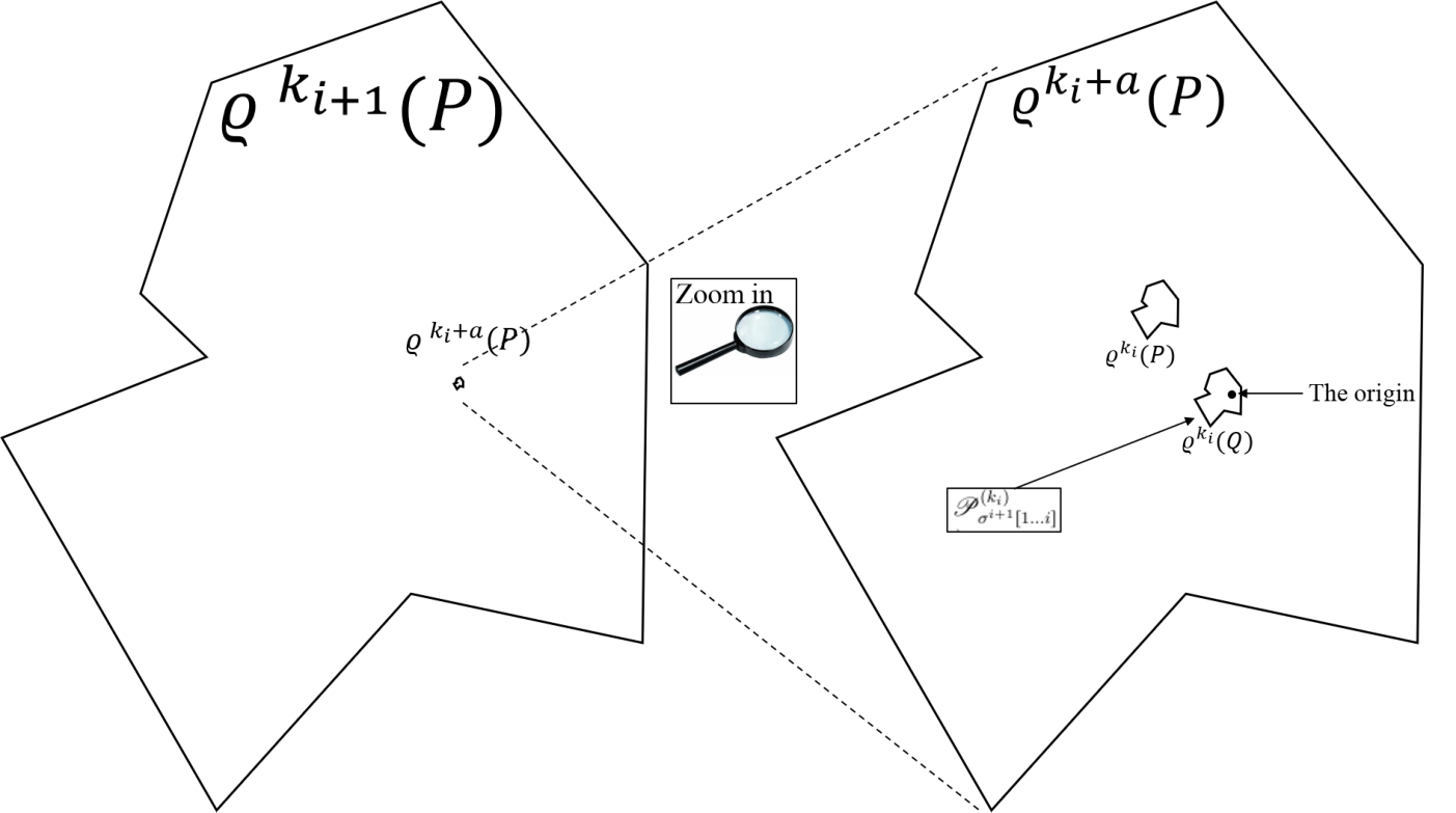
Recall that hh is a multiple of aa and observe that ki+1=hik_{i+1}=h^{i} is a much larger integer than ki+a=hi−1+ak_{i}+a=h^{i-1}+a. If the i+1i+1 letter of σi+1\sigma^{i+1} is PP, denote by 𝒯P\mathscr{T}_{P} the centered copy of ϱ(ki+a)​(P)\varrho^{(k_{i}+a)}(P) inside ϱ(ki+1)​(P)\varrho^{(k_{i+1})}(P) (respectively, if σi+1​(i+1)=Q\sigma^{i+1}(i+1)=Q let 𝒯Q\mathscr{T}_{Q} be the centered copy of ϱ(ki+a)​(Q)\varrho^{(k_{i}+a)}(Q) inside ϱ(ki+1)​(Q)\varrho^{(k_{i+1})}(Q)). A key observation is that positioning 𝒯P\mathscr{T}_{P} (resp. 𝒯Q\mathscr{T}_{Q}) in ℝd{\mathbb{R}}^{d} forces the position of the much larger patch ϱ(ki+1)​(P)\varrho^{(k_{i+1})}(P) (resp. ϱ(ki+1)​(Q)\varrho^{(k_{i+1})}(Q)) that contains it. Consider the centered copy of ϱ(ki)​(P)\varrho^{(k_{i})}(P) or the copy of ϱ(ki)​(Q)\varrho^{(k_{i})}(Q) inside 𝒯P\mathscr{T}_{P}, which exists by Lemma 4.2, depending on whether the ii’th letter of σi+1\sigma^{i+1} is PP or QQ (resp. inside 𝒯Q\mathscr{T}_{Q} consider the centered copy of ϱ(ki)​(Q)\varrho^{(k_{i})}(Q) or the copy of ϱ(ki)​(P)\varrho^{(k_{i})}(P)). One of these two patches, depending on the ii’th letter of σi+1\sigma^{i+1}, is a translated copy of the patch 𝒫σi+1​[1​…​i](ki)\mathscr{P}_{\sigma^{i+1}[1\ldots i]}^{(k_{i})} that we have obtained from the induction hypothesis. We place 𝒯P\mathscr{T}_{P} (resp. 𝒯Q\mathscr{T}_{Q}) so that the above particular copy of ϱ(ki)​(P)\varrho^{(k_{i})}(P) or of ϱ(ki)​(Q)\varrho^{(k_{i})}(Q) in it coincide with 𝒫σi+1​[1​…​i](ki)\mathscr{P}_{\sigma^{i+1}[1\ldots i]}^{(k_{i})}, see Figure 2. The above placement fixes the position of the copy of the patch ϱ(ki+1)​(P)\varrho^{(k_{i+1})}(P) or ϱ(ki+1)​(Q)\varrho^{(k_{i+1})}(Q) from which we have started, and we define this fixed patch to be 𝒫σi+1(ki+1)\mathscr{P}_{\sigma^{i+1}}^{(k_{i+1})}.

Refer to caption
Figure 2. This picture corresponds to the case where the last two letters of σi+1\sigma^{i+1} are Q​PQP and it is done similarly for the other three possible options. The illustration shows how to position the patch ϱ(ki+1)​(P)\varrho^{(k_{i+1})}(P), which is later defined to be 𝒫σi+1(ki+1)\mathscr{P}_{\sigma^{i+1}}^{(k_{i+1})}, providing that we know the position of 𝒫σi+1​[1​…​i](ki)\mathscr{P}_{\sigma^{i+1}[1\ldots i]}^{(k_{i})}, which was given to us by the induction hypothesis. In this picture, as the ii’th letter of σi+1\sigma^{i+1} is QQ, the patch 𝒫σi+1​[1​…​i](ki)\mathscr{P}_{\sigma^{i+1}[1\ldots i]}^{(k_{i})} is a translated copy of ϱ(ki)​(Q)\varrho^{(k_{i})}(Q). We place ϱ(ki+1)​(P)\varrho^{(k_{i+1})}(P) such that the copy of ϱ(ki)​(Q)\varrho^{(k_{i})}(Q) inside the centered copy of ϱ(ki+a)​(P)\varrho^{(k_{i}+a)}(P) in ϱ(ki+1)​(P)\varrho^{(k_{i+1})}(P) (given by Lemma 4.2), coincide with 𝒫σi+1​[1​…​i](ki)\mathscr{P}_{\sigma^{i+1}[1\ldots i]}^{(k_{i})}.

It is left the verify the validity of properties (1), (2) and (3). By the induction hypothesis the origin is contained in 𝒫σi+1​[1​…​i](ki)\mathscr{P}_{\sigma^{i+1}[1\ldots i]}^{(k_{i})}, hence properties (1) and (2) follow directly from the construction. Note that the support of 𝒫σi+1​[1​…​i](ki)\mathscr{P}_{\sigma^{i+1}[1\ldots i]}^{(k_{i})} is indeed disjoint from the boundary of supp​(𝒫σi+1(ki+1))\text{supp}\!\left({\mathscr{P}_{\sigma^{i+1}}^{(k_{i+1})}}\right) by (1) of Lemma 4.2. To see (3), note that by our definition of the notion of a centered copy, the point 𝐱⁡(𝒫σi+1(ki+1))\mathbf{x}\left(\mathscr{P}_{\sigma^{i+1}}^{(k_{i+1})}\right) belongs to 𝒯P\mathscr{T}_{P} (or to 𝒯Q\mathscr{T}_{Q}, depends on σi+1​(i+1)\sigma^{i+1}(i+1)), which also contains the origin. Since for every m∈ℕm\in{\mathbb{N}} the diameter of supp​(ϱm​(P))\text{supp}\!\left({\varrho^{m}(P)}\right) is ξm​diam​(supp​(P))=(λ11/d)m​diam​(supp​(P))\xi^{m}\text{diam}\!\left({\text{supp}\!\left({P}\right)}\right)=(\lambda_{1}^{1/d})^{m}\text{diam}\!\left({\text{supp}\!\left({P}\right)}\right) (see §2.2), and since 𝒯P\mathscr{T}_{P} is a translate of ϱki+a​(P)\varrho^{k_{i}+a}(P), we have

‖𝐱⁡(𝒫σi+1(ki+1))‖≤diam​(supp​(ϱki+a​(P)))=λ1ki+ad​diam​(supp​(P))=c1⋅λ1ki/d.\left\|{\mathbf{x}\left(\mathscr{P}_{\sigma^{i+1}}^{(k_{i+1})}\right)}\right\|\leq\text{diam}\!\left({\text{supp}\!\left({\varrho^{k_{i}+a}(P)}\right)}\right)=\lambda_{1}^{\frac{k_{i}+a}{d}}\text{diam}\!\left({\text{supp}\!\left({P}\right)}\right)=c_{1}\cdot\lambda_{1}^{k_{i}/d}.

In case σi+1​(i+1)=Q\sigma^{i+1}(i+1)=Q, since diam​(supp​(P))=diam​(supp​(Q))\text{diam}\!\left({\text{supp}\!\left({P}\right)}\right)=\text{diam}\!\left({\text{supp}\!\left({Q}\right)}\right), the same computation holds and the proof is complete. ∎

Lemma 4.4.

For every infinite sequence ω∈{P,Q}ℕ\omega\in\{P,Q\}^{\mathbb{N}} there exists a tiling 𝒯ω∈𝕏ϱ\mathcal{T}_{\omega}\in{\mathbb{X}}_{\varrho} so that for every i∈ℕi\in{\mathbb{N}} the tiling 𝒯ω\mathcal{T}_{\omega} contains the patch 𝒫ω⁡[1​…​i](ki)\mathscr{P}_{\omega[1\ldots i]}^{(k_{i})}, defined in Proposition 4.3.

Proof.

Let ω∈{P,Q}ℕ\omega\in\{P,Q\}^{\mathbb{N}}. By (2) of Proposition 4.3, the sequence of patches (𝒫ω⁡[1​…​i](ki))i∈ℕ\left(\mathscr{P}_{\omega[1\ldots i]}^{(k_{i})}\right)_{i\in{\mathbb{N}}} is a nested sequence and by the proof of Proposition 4.3 it exhausts the plane. Thus

Tω:=⋃i∈ℕ𝒫ω⁡[1​…​i](ki)T_{\omega}:=\bigcup_{i\in{\mathbb{N}}}\mathscr{P}_{\omega[1\ldots i]}^{(k_{i})}

is a tiling of ℝd{\mathbb{R}}^{d} and it satisfies the assertion. ∎

Let Ω:={P,Q}ℕ\Omega:=\{P,Q\}^{\mathbb{N}}. Consider the equivalence relation on Ω\Omega in which ω∼ω′\omega\sim\omega^{\prime} if the set {i∈ℕ∣w⁡(i)≠w′​(i)}\{i\in{\mathbb{N}}\mid w(i)\neq w^{\prime}(i)\} is finite. Since every equivalence class in this relation is countable, the cardinality of a set Ω~⊂Ω\widetilde{\Omega}\subset\Omega of equivalence class representatives is 2ℵ02^{\aleph_{0}}. We fix such a set of representatives Ω~\widetilde{\Omega}, then the following lemma completes the proof of Theorem 1.1.

Lemma 4.5.

Let ω,η∈Ω~\omega,\eta\in\widetilde{\Omega} be two distinct sequences, then the tilings 𝒯ω\mathcal{T}_{\omega} and 𝒯η\mathcal{T}_{\eta}, which are defined in Lemma 4.4, are BD-non-equivalent.

Proof.

Since ω\omega and η\eta are in Ω~\widetilde{\Omega}, and they are distinct, they differ at infinitely many places. Let (im)m=1∞(i_{m})_{m=1}^{\infty} be an increasing sequence so that ω⁡(im)≠η⁡(im)\omega(i_{m})\neq\eta(i_{m}) for every mm. We set kimk_{i_{m}} as in (4.6) and apply Corollary 2.7 with the sequence of sets (Am)m∈ℕ(A_{m})_{m\in{\mathbb{N}}} defined by

Bm:=supp(ϱkim(P)𝐱⁡(P)),Am:=⋃{C(x)∈𝒬d∣Bm∩C(x)≠∅}(see §2.3).B_{m}:=\text{supp}\!\left({\varrho^{k_{i_{m}}}(P)_{\mathbf{x}(P)}}\right),\qquad A_{m}:=\bigcup\left\{C(x)\in\mathcal{Q}_{d}\mid B_{m}\cap C(x)\neq\varnothing\right\}\quad(\text{see }\lx@sectionsign\ref{subsec:BD}).

By (3) of Proposition 4.3 we have

‖𝐱⁡(𝒫ω⁡[1​…​im](kim))‖,‖𝐱⁡(𝒫η⁡[1​…​im](kim))‖≤c1⋅λ1kim−1d.\left\|{\mathbf{x}\left(\mathscr{P}_{\omega[1\ldots i_{m}]}^{(k_{i_{m}})}\right)}\right\|,\left\|{\mathbf{x}\left(\mathscr{P}_{\eta[1\ldots i_{m}]}^{(k_{i_{m}})}\right)}\right\|\leq c_{1}\cdot\lambda_{1}^{\frac{k_{i_{m}-1}}{d}}.

Since BmB_{m} and supp​(𝒫ω⁡[1​…​im](kim))\text{supp}\!\left({\mathscr{P}_{\omega[1\ldots i_{m}]}^{(k_{i_{m}})}}\right) differ by a translation and since 𝐱⁡(ϱkim​(P)𝐱⁡(P))=0\mathbf{x}(\varrho^{k_{i_{m}}}(P)_{\mathbf{x}(P)})=0 by definition, we deduce that

Bm△supp(𝒫ω⁡[1​…​im](kim))⊂{𝐱∈ℝd∣∃𝐲∈∂Bm,‖𝐱−𝐲‖≤c1⋅λ1kim−1d},B_{m}\ \triangle\ \text{supp}\!\left({\mathcal{P}_{\omega[1\ldots i_{m}]}^{(k_{i_{m}})}}\right)\subset\left\{\mathbf{x}\in{\mathbb{R}}^{d}\mid\exists\mathbf{y}\in\partial B_{m},\ \left\|{\mathbf{x}-\mathbf{y}}\right\|\leq c_{1}\cdot\lambda_{1}^{\frac{k_{i_{m}-1}}{d}}\right\},

and therefore

Am△supp(𝒫ω⁡[1​…​im](kim))⊂{𝐱∈ℝd∣∃𝐲∈∂Am,‖𝐱−𝐲‖≤d⋅c1⋅λ1kim−1d}=def𝒮.A_{m}\ \triangle\ \text{supp}\!\left({\mathcal{P}_{\omega[1\ldots i_{m}]}^{(k_{i_{m}})}}\right)\subset\left\{\mathbf{x}\in{\mathbb{R}}^{d}\mid\exists\mathbf{y}\in\partial A_{m},\ \left\|{\mathbf{x}-\mathbf{y}}\right\|\leq\sqrt{d}\cdot c_{1}\cdot\lambda_{1}^{\frac{k_{i_{m}-1}}{d}}\right\}{\,\stackrel{{\scriptstyle\mathrm{def}}}{{=}}\,}\mathcal{S}.

using e.g. [L, Lammas 2.1 & 2.2], μd​(𝒮)≤c⁡(d)⋅c1d⋅λ1kim−1⋅μd−1​(∂Am)\mu_{d}\left(\mathcal{S}\right)\leq c(d)\cdot c_{1}^{d}\cdot\lambda_{1}^{k_{i_{m}-1}}\cdot\mu_{d-1}(\partial A_{m}) and hence

μd​(Am​△​supp​(𝒫ω⁡[1​…​im](kim)))≤c⁡(d)⋅c1d⋅λ1kim−1⋅μd−1​(∂Am),\mu_{d}\left(A_{m}\ \triangle\ \text{supp}\!\left({\mathcal{P}_{\omega[1\ldots i_{m}]}^{(k_{i_{m}})}}\right)\right)\leq c(d)\cdot c_{1}^{d}\cdot\lambda_{1}^{k_{i_{m}-1}}\cdot\mu_{d-1}(\partial A_{m}),

where c⁡(d)c(d) is a constant that depends on the dimension dd. Bounding the number of tiles in a region by the volume of the region divided by the smallest volume of a prototile, we obtain a constant c2>0c_{2}>0 that depends on dd, aa, PP and ϱ\varrho so that

(4.7) |#​[Am]𝒯ω−#​𝒫ω⁡[1​…​im](kim)|≤#​[Am​△​supp​(𝒫ω⁡[1​…​im](kim))]𝒯ω≤c2⋅λ1kim−1⋅μd−1​(∂Am).\left|{\#[A_{m}]^{\mathcal{T}_{\omega}}-\#\mathcal{P}_{\omega[1\ldots i_{m}]}^{(k_{i_{m}})}}\right|\leq\#\left[A_{m}\ \triangle\ \text{supp}\!\left({\mathcal{P}_{\omega[1\ldots i_{m}]}^{(k_{i_{m}})}}\right)\right]^{\mathcal{T}_{\omega}}\leq c_{2}\cdot\lambda_{1}^{k_{i_{m}-1}}\cdot\mu_{d-1}(\partial A_{m}).

The above computations hold for 𝒫η⁡[1​…​im](kim)\mathcal{P}_{\eta[1\ldots i_{m}]}^{(k_{i_{m}})} instead of 𝒫ω⁡[1​…​im](kim)\mathcal{P}_{\omega[1\ldots i_{m}]}^{(k_{i_{m}})} as well, and so we also have

(4.8) |#​[Am]𝒯η−#​𝒫η⁡[1​…​im](kim)|≤c2⋅λ1kim−1⋅μd−1​(∂Am).\left|{\#[A_{m}]^{\mathcal{T}_{\eta}}-\#\mathcal{P}_{\eta[1\ldots i_{m}]}^{(k_{i_{m}})}}\right|\leq c_{2}\cdot\lambda_{1}^{k_{i_{m}-1}}\cdot\mu_{d-1}(\partial A_{m}).

Combining (4.7) and (4.8) we obtain that

(4.9) |#​[Am]𝒯ω−#​[Am]𝒯η|≥|#​𝒫ω⁡[1​…​im](kim)−#​𝒫η⁡[1​…​im](kim)|−2​c2⋅λ1kim−1⋅μd−1​(∂Am).\left|{\#[A_{m}]^{\mathcal{T}_{\omega}}-\#[A_{m}]^{\mathcal{T}_{\eta}}}\right|\geq\left|{\#\mathcal{P}_{\omega[1\ldots i_{m}]}^{(k_{i_{m}})}-\#\mathcal{P}_{\eta[1\ldots i_{m}]}^{(k_{i_{m}})}}\right|-2c_{2}\cdot\lambda_{1}^{k_{i_{m}-1}}\cdot\mu_{d-1}(\partial A_{m}).

Since ω⁡(im)≠η⁡(im)\omega(i_{m})\neq\eta(i_{m}), and by Lemma 4.1 and property (1) of Proposition 4.3, we have

(4.10) |#​𝒫ω⁡[1​…​im](kim)−#​𝒫η⁡[1​…​im](kim)|≥c0​|λt|kim.\left|{\#\mathcal{P}_{\omega[1\ldots i_{m}]}^{(k_{i_{m}})}-\#\mathcal{P}_{\eta[1\ldots i_{m}]}^{(k_{i_{m}})}}\right|\geq c_{0}\left|{\lambda_{t}}\right|^{k_{i_{m}}}.

Relying on (2.1), let c3>0c_{3}>0 be ℋd−1​(∂supp​(P))\mathcal{H}_{d-1}(\partial\text{supp}\!\left({P}\right)) times a constant that depends on dd such that

(4.11) μd−1​(∂Am)≤c3​(ξkim)d−1=c3​(λ1(d−1)/d)kim,\mu_{d-1}(\partial A_{m})\leq c_{3}\left(\xi^{k_{i_{m}}}\right)^{d-1}=c_{3}\left(\lambda_{1}^{(d-1)/d}\right)^{k_{i_{m}}},

then by (4.10) and 4.11 we have

(4.12) |#​𝒫ω⁡[1​…​im](kim)−#​𝒫η⁡[1​…​im](kim)|/μd−1​(∂Am)≥c0c3​(|λt|λ1(d−1)/d)kim.\left|{\#\mathcal{P}_{\omega[1\ldots i_{m}]}^{(k_{i_{m}})}-\#\mathcal{P}_{\eta[1\ldots i_{m}]}^{(k_{i_{m}})}}\right|/\mu_{d-1}(\partial A_{m})\geq\frac{c_{0}}{c_{3}}\left(\frac{\left|{\lambda_{t}}\right|}{\lambda_{1}^{(d-1)/d}}\right)^{k_{i_{m}}}.

Note that Am∈𝒬d∗A_{m}\in\mathcal{Q}_{d}^{*}, thus plugging (4.9) and (4.12) into (2.5) we obtain that

(4.13) |#​[Am]𝒯ω−#​[Am]𝒯η|μd−1​(∂Am)≥c0c3​(|λt|λ1(d−1)/d)kim−2​c2​λ1kim−1.\frac{\left|{\#[A_{m}]^{\mathcal{T}_{\omega}}-\#[A_{m}]^{\mathcal{T}_{\eta}}}\right|}{\mu_{d-1}(\partial A_{m})}\geq\frac{c_{0}}{c_{3}}\left(\frac{\left|{\lambda_{t}}\right|}{\lambda_{1}^{(d-1)/d}}\right)^{k_{i_{m}}}-2c_{2}\lambda_{1}^{k_{i_{m}-1}}.

In view of (4.6),

(|λt|λ1(d−1)/d)kim=(|λt|λ1(d−1)/d)him−1,λ1kim−1=(λ11h)him−1​andλ11h<|λt|λ1(d−1)/d,\left(\frac{\left|{\lambda_{t}}\right|}{\lambda_{1}^{(d-1)/d}}\right)^{k_{i_{m}}}=\left(\frac{\left|{\lambda_{t}}\right|}{\lambda_{1}^{(d-1)/d}}\right)^{h^{i_{m}-1}},\lambda_{1}^{k_{i_{m}-1}}=\left(\lambda_{1}^{\frac{1}{h}}\right)^{h^{i_{m}-1}}\text{and}\quad\lambda_{1}^{\frac{1}{h}}<\frac{\left|{\lambda_{t}}\right|}{\lambda_{1}^{(d-1)/d}},

which implies that the quantity on the right hand side of (4.13) tends to infinity with mm. Then by Corollary 2.7, the proof of the lemma and hence of Theorem 1.1 is complete. ∎

References

  • [ACG] J. Aliste-Prieto, D. Coronel, J. M. Gambaudo, Linearly repetitive Delone sets are rectifiable, Ann. Inst. H. Poincaré Anal. Non Linéaire 30 (2), 275-290, (2013).
  • [BG] M. Baake, U. Grimm, Aperiodic order. Volume 1: A mathematical invitation, Cambridge University Press, Cambridge (2013).
  • [DSS] W. A. Deuber, M. Simonovits, V. T. Sós. A note on paradoxical metric spaces, Studia Scientiarum Mathematicarum Hungarica 30 (1), 17-24, (1995).
  • [DO1] M. Duneau, C. Oguey. Displacive transformations and quasicrystalline symmetries, Journal de Physique 51 (1), 5-19, (1990).
  • [DO2] M. Duneau, C. Oguey. Bounded interpolation between lattices, Journal of Physics A: Mathematical and General 24, 461-475, (1991).
  • [FSS] D. Frettlöh, Y. Smilansky, Y. Solomon, Bounded Displacement Non-Equivalence In Substitution Tilings, arxiv:1907.01597, (2019).
  • [HKK] A. Haynes, M. Kelly, H. Koivusalo, Constructing bounded remainder sets and cut-and-project sets which are bounded distance to lattice, II, Indagationes Mathematicae 28 (1), 138-144, (2017).
  • [HKW] A. Haynes, M. Kelly, B. Weiss, Equivalence relations on separated nets arising from linear toral flows, Proc. Lond. Math. Soc. 109 (5), 1203-1228, (2014).
  • [HK] A. Haynes, H. Koivusalo, Constructing bounded remainder sets and cut-and-project sets which are bounded distance to lattice, Israel J. Math. 212, 189-201, (2016).
  • [L] M. Laczkovich, Uniformly spread discrete sets in ℝd{\mathbb{R}}^{d}, J. Lond. Math. Soc. 46 (2), 39-57, (1992).
  • [Mag] A. N. Magazinov, The family of bi-Lipschitz classes of Delone sets in Euclidean space has the cardinality of the continuum, Proc. of the Steklov. Inst. of Math. 275, 87-98, (2011).
  • [Mat] P. Mattila, Geometry of sets and measures in Euclidean spaces. Fractals and rectifiability, volume 44 of Cambridge Studies in Advanced Mathematics. Cambridge University Press, Cambridge, (1995).
  • [Q] M. Queffélec, Substitution dynamical systems - spectral analysis, Lecture Notes in Mathematics, vol. 1294, Springer-Verlag, Berlin, 1987.
  • [SS] Y. Smilansky, Y. Solomon, Multiscale substitution tilings, arxiv:2003.11735, (2020).
  • [S1] Y. Solomon, Substitution tilings and separated nets with similarities to the integer lattice, Israel J. Math. 181, 445-460, (2011).
  • [S2] Y. Solomon, A simple condition for bounded displacement, J. Math. Anal. Appl. 414, 134-148, (2014).