A practical Response Adaptive Block Randomization (RABR) design with analytic type I error protectionPublication type: RESEARCH ARTICLE

Randomized clinical trials (RCTs) remain the gold standard for understanding the effect of a treatment or other intervention relative to placebo or standard of care. (Diamond et al. 2015; Wu et al. 2017; Barnhart et al. 2018) To make the trial more efficient and ethical, confirmatory adaptive designs become more widely acceptable and popular to allow flexible interim modifications in the ongoing trials using unblinded data without compromising the type I error rate. (FDA 2019; United States Congress 2016; Bretz et al. 2009) An appealing branch is the response adaptive randomization (RAR) design, where the chance of a newly enrolled subject being assigned to a treatment arm varies over the course of the trial based on accumulating outcome data for subjects previously enrolled. (FDA 2019) Statistical, ethical, and pragmatic rationales support the advantage of using RAR as more subjects are being assigned to the more promising treatment arms. As a popular method of RAR, Doubly Adaptive Biased Coin Design (DBCD) accounts for both the current sample proportion and a desired allocation function. (Eisele 1994; Hu and Rosenberger 2006; Williamson and Villar 2020) Covariate-adjusted RAR designs are also receiving more attention recently. (Hu et al. 2015; Zhu and Hu 2018)

However, in industry-sponsored confirmatory clinical studies to evaluate drug efficacy and safety, randomization ratios and targeted sample sizes of treatment groups are typically pre-specified in study protocols prior to conducting the clinical trial to meet regulatory requirements. ICH E3 1996 As demonstrated in Section 5 on simulations studies, although DBCD allows one to adjust tuning parameters in allocation functions based on assumptions at the study design stage, DBCD may potentially miss an agreed randomization target if observed data deviate. This is more challenging when there is limited prior knowledge on the efficacy of treatment regimes, as in the case study we considered in Section 6.

To address this challenge, we propose a Response Adaptive Block Randomization (RABR) design motived by Wang and Cui, Wang and Cui 2007 and Cui et al., Cui et al. 2020 where subjects are adaptively randomized to different treatment groups based on the order of their standardized effect sizes and a pre-specified block randomization vector. As shown in simulation studies in Section 5 and the case study in Section 6, our RABR is more robust than DBCD in achieving a desired final sample size per group under varying underlying treatment effects. By effectively increasing the sample size of the selected treatment group to target levels, and decreasing the number of patients randomized to worse performing groups, our proposed RABR also has a higher power of detecting a significant treatment effect than DBCD. Moreover, the built-in block randomization feature of RABR facilitates its implementation in practice, in the sense that Interactive Response Technology (IRT) schedules can be specified in advance. While the application of RAR in blocks has been studied in some previous articles in the context of two-group comparisons with a binary endpoint, (Magirr 2011; Karrison et al. 2003) our approach is proposed to accommodate multi-arm trials with broader data types and to achieve targeted final sample size for the selected treatment group. Another contribution of our work is to analytically prove that the one-sided type I error rate for pairwise comparison is controlled at a nominal significance level by using the usual unweighted test statistic, which does not rely on large sample approximation despite the data-driven randomization process. The unweighted statistics are easier to compute than weighted statistics, (Cui et al. 2020; Cui et al. 1997; Cui et al. 1999) and they are a good alternative to the weighted combination test (Cui et al. 2020) particularly when multiple treatment groups are presented and complicated multiplicity adjustment is needed.

The remainder of this article is organized as follows. In Section 2, we review the DBCD with a continuous endpoint, which will be used to compare with the proposed design and analysis. In Section 3, we introduce our proposed RABR. The analytic type I error rate protection in pairwise comparison is proved in Section 4. Simulations are performed to evaluate type I error and power under various scenarios in Section 5. As a practical example, we further re-design a confirmatory trial for treating tuberous sclerosis complex with RABR at Section 6. Concluding remarks are provided in Section 7.

In this section, we review the Doubly Adaptive Biased Coin Designs (DBCD). Hu and Rosenberger 2006 Let us consider a clinical trial with a continuous endpoint, where the response $X^{\left(g\right)}_{i}$ for subject $i$ in treatment group $g$ follows independent normal distribution with mean $\mu_{g}$ and variance $\sigma_{g}^{2}$,

for $g=0$ labeling placebo and $g=1,\ldots,m$ for $m$ treatment groups. We assume that a higher response is favorable, and the response of each subject is observed right after its enrollment in the study.

After a burn-in period where $M$ subjects have been equally randomized to $m+1$ groups, the study adjusts the randomization probability to each treatment group $g$ ($g=0,1,\ldots,m$) based on the following allocation function:

where $\eta$ is a non-negative tuning parameter controlling randomness of randomization probabilities. The asymptotic allocation variance is a monotone decreasing function of $\eta$, and usually $\eta=2$ is chosen in practice. (Hu and Rosenberger 2006) In $a_{g}(\eta,\theta_{g},\tau_{g})$, $\theta_{g}$ is the proportion of subjects that have been randomized to group $g$ so far, and $\tau_{g}$ is the targeting allocation probability for group $g$. In this article, we consider $\tau_{g}$ in the following form:

which is a direct generalization of the allocation function with a continuous endpoint of treatment failure in two-group comparison (Biswas and Mandal 2004) to a study with multiple treatment groups. The tuning parameter $\lambda$ needs to be pre-specified.

We further use $\widehat{\tau_{g}}$ to denote an estimate of $\tau_{g}$ by replacing $\mu_{g}$ and $\sigma_{g}$ by their consistent estimators. At each interim checkpoint, the adaptive randomization probability for treatment group $g$ is $a_{g}(\eta,\theta_{g},\widehat{\tau_{g}})$. In the context of two-group comparison, it can be shown that $\widehat{\tau_{g}}$ and $\theta_{g}$ converge to $\tau_{g}$ almost surely, and with an asymptotic bivariate normal distribution under certain regulatory conditions. (Hu and Rosenberger 2006) When the sample size is large enough, the study reaches stabilized randomization probabilities to each group $g$ at $\tau_{g}$. Therefore, asymptotically, a level $\alpha$ test for a non-adaptive design is also valid to control the pairwise comparison error rate at $\alpha$. One can further use certain multiple test procedures to control the family-wise error rate (FWER).

Challenges exist for this type of design to robustly achieve a desired sample size for the selected arm and placebo with a given $\lambda$ under different underlying responses. This issue is further studied in Section 5. Moreover, block randomization is generally not available given the functional form of $a_{g}$ in (2). The trial may end up with an undesired final proportion per group, especially when the total sample size is relatively small. In the next section, we introduce our proposed Response Adaptive Block Randomization (RABR) Design as an alternative option along with an analytic type I error protection.

As a starting point, let us consider a simple two-stage study design with one interim adaptation on the randomization. The generalization to multiple stages is illustrated in the following Theorem 4.4. In stage 1, there are $N_{1}^{\left(g\right)}$ subjects that have been recruited to group $g$ with sample mean $\hbox{\vbox{\hrule height=0.5pt\kern 2.15277pt\hbox{\kern-1.00006pt$X$\kern-1.00006pt}}}_{1}^{\left(g\right)}=\sum_{i=1}^{N_{1}^{\left(g\right)}}X_{i}^{\left(g\right)}/N_{1}^{\left(g\right)}$, for $g=0,1,\ldots,m$. Further denote $\boldsymbol{X}_{1}^{\left(g\right)}=\left\{X_{1}^{\left(g\right)},\ldots,X_{N_{1}^{\left(g\right)}}^{\left(g\right)}\right\}$ as the vector of responses in group $g$ at stage 1. Similar to the DBCD as described in Section 2, we utilize stage 1 as a burn-in period, where equal randomization is adopted on the placebo and $m$ treatment group: $N_{1}^{\left(0\right)}=N_{1}^{\left(1\right)}=\cdots=N_{1}^{\left(m\right)}$. The burn-in size $M$ is equal to $\sum_{g=0}^{m}N_{1}^{\left(g\right)}$. Correspondingly, $N_{2}^{\left(g\right)}$ and $\hbox{\vbox{\hrule height=0.5pt\kern 2.15277pt\hbox{\kern-1.00006pt$X$\kern-1.00006pt}}}_{2}^{\left(g\right)}$ are notations for sample size and sample mean in group $g$ at stage 2. We use $\hbox{\vbox{\hrule height=0.5pt\kern 2.15277pt\hbox{\kern-1.00006pt$X$\kern-1.00006pt}}}^{\left(g\right)}$ and $N^{\left(g\right)}$ to denote the sample mean and sample size of group $g$ in the whole study, for $g=0,1,\cdots,m$. In this article, we consider studies with either $m=2$ or $3$ active treatment groups with generalization to $m>3$, as briefly discussed in Section 7.

Having observed the first stage data $\boldsymbol{D}_{1}=\left\{\boldsymbol{X}_{1}^{\left(0\right)},\boldsymbol{X}_{1}^{\left(1\right)},\ldots,\boldsymbol{X}_{1}^{\left(m\right)}\right\}$, we adjust the randomization ratios of $m$ treatment groups in a data-driven manner by assigning more subjects to the more promising dose(s). Let vector $\boldsymbol{r}=(r_{0},r_{1},r_{2},\ldots,r_{m})$ denote a pre-specified block randomization vector for our design, where $r_{g}$ are integers satisfying $r_{1}\geq r_{2}\geq\cdots\geq r_{m}$ for $g=1,\ldots,m$. The block size $B$ is equal to $\sum_{g=0}^{m}r_{g}$. The first element $r_{0}$ in $\boldsymbol{r}$ specifies the number of subjects being randomized to the placebo group in one block. Therefore, the randomization probability to the placebo is fixed at $r_{0}$ out of $B$. The rest of the $m$ elements in $\boldsymbol{r}:$ $r_{1},\ldots,r_{m}$ are assigned to $m$ treatment groups based on a decreasing order of the standardized response denoted as $R_{g}$,

where $\widehat{\sigma}_{g}$ is the sample standard deviation of data $\boldsymbol{X}_{1}^{\left(g\right)}$, for $g=1,\ldots,m$. That is to say, the group with the largest standardized observed mean in the first stage gets the highest probability of being randomized in the second stage ($r_{1}$ out of $B$). The functional form in (4) is appealing as it is on the same scale of the final test statistics, and it also eases our analytic proof of pairwise type I error rate control at Section 4.1. Even if $\boldsymbol{r}$ is pre-specified, its assignment to each treatment group $g$, $g=1,\ldots,m$ is dependent on the previous stage data $\boldsymbol{D}_{1}$.

For demonstration, let’s consider a study with $m=2$ active doses with $g=0,1,2$ denoting the placebo, the low dose and the high dose group, respectively. Without loss of generality, we focus on the low dose $g=1$ for illustration. We use $N_{2}^{\left(1\right)}(\boldsymbol{D}_{1})$ to denote the sample size in treatment group $g=1$ at the second stage. It takes the value $\beta_{1}N_{2}^{\left(0\right)}$ if $\left\{N_{1}^{\left(1\right)}\right\}^{1/2}\>\>\hbox{\vbox{\hrule height=0.5pt\kern 2.15277pt\hbox{\kern-1.00006pt$X$\kern-1.00006pt}}}_{1}^{\left(1\right)}/\widehat{\sigma}_{1}\geq\left\{N_{1}^{\left(2\right)}\right\}^{1/2}\>\>\hbox{\vbox{\hrule height=0.5pt\kern 2.15277pt\hbox{\kern-1.00006pt$X$\kern-1.00006pt}}}_{1}^{\left(2\right)}/\widehat{\sigma}_{2}$, and $\beta_{2}N_{2}^{\left(0\right)}$ otherwise, where $\beta_{1}=r_{1}/r_{0}$ and $\beta_{2}=r_{2}/r_{0}$. Essentially, subjects are more likely to be assigned to the low dose in the second stage if its response is more promising than that in the high dose based on $\boldsymbol{D}_{1}$. If $\beta_{1}=\beta_{2}$, then it degenerates to a non-adaptive design with equal randomization. We simplify the notation of $N_{2}^{\left(1\right)}(\boldsymbol{D}_{1})$ as $N_{2}^{\left(1\right)}$.

To illustrate randomization procedures in RABR following some related discussion in Cui et al.,Cui et al. 2020 we consider a study to evaluate low dose $L$ and high dose $H$ versus placebo $P$ with $\boldsymbol{r}=(2,3,1)$ of block size $B=6$ in Figure 1, where 2 out of 6 is for placebo and 3 out of 6 is for the better performing group. Before the current trial conduct, we first build three sets of randomization schedules: Schedule $Q_{1}$ with equal randomization probabilities, Schedule $Q_{2}$ with a higher randomization probability for $L$, and Schedule $Q_{3}$ with high probability for $H$. During the burn-in period, Schedule $Q_{1}$ is activated to achieve equal randomization. For each subject enrolled after burn-in period, the standardized responses $R_{L}$ and $R_{H}$ in (4) are calculated based on accumulated data for $L$ and $H$, respectively. If $R_{L}\geq R_{H}$ which means that $L$ is performing better, then Schedule $Q_{2}$ is activated with a higher probability of $3$ out $6$ to assign the next subject to this dose, and vice versa. In our proposed RABR, there are several design parameters involved, for example the burn-in size $M$, block size $B$, allocation vector $\boldsymbol{r}$ and total sample size $N$. Their choices are relatively flexible, but have to be pre-specified in the protocol or Statistical Analysis Plan (SAP). We provide more discussion on how to choose values for these parameters to meet specific study objectives in Section 5.2 and 6. The impact of design parameters are also evaluated later in Section 5.2.

By simulations, we study the type I error rate of RABR design with a continuous endpoint at Section 5.1. The final allocations and power are further compared with DBCD at Section 5.2 under several response assumptions.

Consider a clinical trial with three active treatment dosing groups, $D_{1}$, $D_{2}$, $D_{3}$, and a placebo. There are $M=60$ subjects being recruited in the burn-in period with fixed equal randomization probabilities and a subsequent $60$ subjects being adaptively and sequentially randomized. Therefore, the total sample size is $N=120$. We utilize the step-down Dunnett test to control multiplicity. (Bretz et al. 2016) At the final efficacy analysis stage, the dosing group with the smallest step-down Dunnett adjusted $p$-value is chosen as the selected one. Its efficacy is further confirmed if its adjusted $p$-value is smaller than $\alpha$. We use $S_{1}$ to denote the selected treatment group, and use $S_{2}$ and $S_{3}$ for the second best and worst groups.

The study objective is to identify and confirm the efficacy of the best performing dose $S_{1}$ with FWER controlled at one-sided $\alpha=2.5\%$, while achieving a desired final sample size for that group and the placebo. Note that the choice of $S_{1}$ from $D_{1}$, $D_{2}$ and $D_{3}$ depends on the data, and does not necessarily correspond to a particular dosing group.

Examining Everolimus in a Study of Tuberous Sclerosis Complex (EXIST-3) evaluated two dosing regimens of adjunctive everolimus compared with placebo for treatment-resistant focal-onset seizures in tuberous sclerosis complex. (French et al. 2016) In this phase 3, randomised, double-blinded, placebo-controlled study, eligible patients were equally and randomly assigned (1:1:1) to receive placebo, 3-7 ng/mL everolimus (low exposure) and 9-15 ng/mL (high exposure) everolimus with block randomization (block size of six). The primary endpoint was the proportion of patients achieving at least $50\%$ reduction in seizure frequency during a 12-week maintenance period, and therefore a larger proportion corresponds to a better outcome. A Bonferroni procedure was used to ensure an one-sided FWER at $2.5\%$.

In the absence of previous dose-finding studies in this indication, the sample size of this phase 3 trial was determined to provide at least $90\%$ power to detect a difference in response rate from $15\%$ on placebo to $35\%$ in each of the two everolimus treatment groups based on literature review. (French et al. 2016) With limited prior knowledge to distinguish the efficacy of two treatment groups, equal randomization is a reasonable choice for this type of non-adaptive confirmatory trial. After completing this study, the results revealed that the response rate was $15.1\%$ with placebo compared with $28.2\%$ ($p=0.0077$) for low exposure everolimus and $40.0\%$ ($p<0.0001$) for high-exposure by using Cochran-Mantel-Haenszel Chi-square tests stratified by four age subgroups. More subjects could have been recruited to the high-exposure group due to a better efficacy profile and the fact that two doses have similar safety profiles. (French et al. 2016) In the remainder of this section, we re-design this non-adaptive design by our proposed RABR to assign more subjects to the better performing treatment group, and to reach the target sample size.

For demonstration purposes, we simulate the trial with instant response based on the above underlying response rates with no stratification factor and a total sample size of $180$. Following notations in Section 5, we use $D_{1}$ to denote the low exposure group, $D_{2}$ for the high exposure group. The selected treatment group $S_{1}$ is the arm between $D_{1}$ and $D_{2}$ with a smaller $p$-value in the test of proportion at the final analysis stage, and $S_{2}$ is the other arm as the worse performing treatment group. Suppose that the target sample size for the placebo and the selected arm $S_{1}$ is $72$. With a burn-in size $M=90$ with equal randomization, our RABR targets the desired allocations using an adaptive randomization vector $\boldsymbol{r}=(7,7,1)$. In DBCD, we consider a generalization of the Neyman allocation (Hu and Rosenberger 2006) as the target allocation function,

where $q^{(g)}$ denotes the response rate in group $g$, and $g=0$ corresponds to placebo, $g=1$ for $D_{1}$, and $g=2$ for $D_{2}$. In all three methods considered (fixed randomization design, RABR and DBCD), the test of proportion is conducted to compare each exposure group versus placebo. The Bonferroni procedure is used to adjust for multiplicity.

We first study the type I error rate when using the unweighted proportion test under our RABR design. Based on simulations with $100,000$ iterations, the one-sided error rates for two pairwise comparisons are lower than $\alpha=2.5\%$ under a comprehensive scan of the null response rate. The conservativeness of type I error rate is the consistent with the findings of continuous endpoints in Table 1, and is proved in Supplemental Materials Section 3. The probability of rejecting at least one elementary null hypothesis by the Bonferroni procedure is also upper bounded by $\alpha$ (Figure 3).

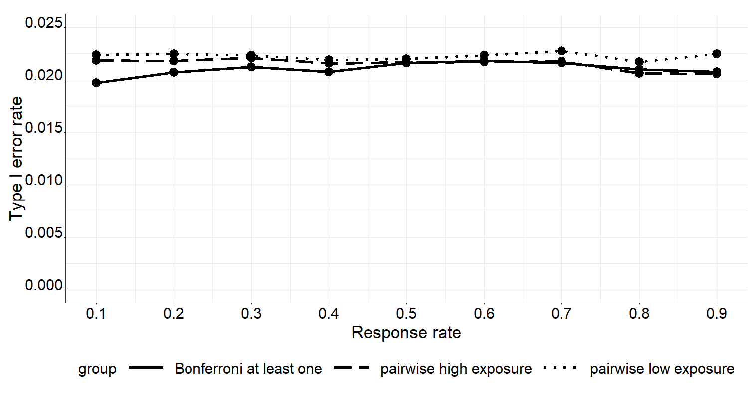
Next we evaluate power and operating characteristics of the three methods in Table 5. Our RABR has the highest overall power at $86.22\%$, compared to the non-adaptive design with fixed randomization at $82.57\%$ and DBCD at $81.97\%$ (Table 5). The probability of selecting and confirming the efficacy of the right dose ($D_{2}$; high exposure group) is also the highest ($78.40\%$). Another objective for two adaptive designs is to reach a target sample size of $72$ for both the placebo and the selected arm $S_{1}$. RABR achieves an average sample size of $72.02$ for the placebo and $69.93$ for $S_{1}$, which are closer to the target sample size than DBCD with $50.33$ for the placebo and $67.69$ for $S_{1}$. We observe that in general RABR has the largest variation in average sample size while fixed randomization has the smallest one based on standard deviation reported in parenthesis.

References

- Diamond et al. (2015) Diamond, M. P., Legro, R. S., Coutifaris, C., Alvero, R., Robinson, R. D., Casson, P., Christman, G. M., Ager, J., Huang, H., Hansen, K. R., Baker, V., Usadi, R., Seungdamrong, A., Bates, G. W., Rosen, R. M., Haisenleder, D., Krawetz, S. A., Barnhart, K., Trussell, J.C., Ohl, D., Jin, Y., Santoro, N., Eisenberg, E., Zhang, H. (2015). Letrozole, gonadotropin, or clomiphene for unexplained infertility. New England Journal of Medicine, 373(13), 1230-1240.
- Wu et al. (2017) Wu, X., Stener-Victorin, E., Kuang, H. Y., Ma, H. L., Gao, J. S., Xie, L. Z., Hou, L. H., Hu, Z. X., Shao, X. G., Ge, J., Zhang, J. F., Xue, H. Y., Xu, X. F., Liang, R. N., Ma, H. X., Yang, H. W., Li, W. L., Huang, D. M., Sun, Y,, Hao, C. F., Du, S. M., Yang, Z. W., Wang, X., Yan, Y., Chen, X. H., Fu, P., Ding, C. F., Gao, Y. Q., Zhou, Z. M., Wang, C. C., Wu, T. X., Liu, J. P., Ng, E. H. Y., Legro, R. S., Zhang, H., PCOSAct Study Group (2017). Effect of acupuncture and clomiphene in chinese women with polycystic ovary syndrome: A randomized clinical trial. JAMA, 317, 2502-2514.
- Barnhart et al. (2018) Barnhart, K. T., Sammel, M. D., Stephenson, M., Robins, J., Hansen, K. R., Youssef, W. A., Santoro, N., Eisenberg, E. and Zhang, H. (2018). Optimal treatment for women with a persisting pregnancy of unknown location, a randomized controlled trial: The ACT-or-NOT trial. Contemporary Clinical Trials, 145-151.
- FDA (2019) Adaptive design clinical trials for drugs and biologics guidance for industry. Food and Drug Administration Website. https://www.fda.gov/regulatory-information/search-fda-guidance-documents/adaptive-design-clinical-trials-drugs-and-biologics-guidance-industry. Published 2019. Accessed April 13, 2021.
- United States Congress (2016) H.R.34 21st century cures act. United States Congress Website. https://www.congress.gov/bill/114th-congress/house-bill/34. Published 2016. Accessed April 13, 2021.
- Bretz et al. (2009) Bretz, F., Koenig, F., Brannath, W., Glimm, E., and Posch, M. (2009). Adaptive designs for confirmatory clinical trials. Statistics in Medicine, 28, 1181-1217.
- Eisele (1994) Eisele, J. R. (1994). The doubly adaptive biased coin design for sequential clinical trials. Journal of Statistical Planning and Inference, 38, 249-261.
- Hu and Rosenberger (2006) Hu, F., and Rosenberger, W. F. (2006). The theory of response-adaptive randomization in clinical trials John Wiley and Sons.
- Williamson and Villar (2020) Williamson, S. F., and Villar, S. S. (2020). A response‐adaptive randomization procedure for multi‐armed clinical trials with normally distributed outcomes. Biometrics, 76(1), 197-209.
- Hu et al. (2015) Hu, J., Zhu, H., and Hu, F. (2015). A unified family of covariate-adjusted response-adaptive designs based on efficiency and ethics. Journal of the American Statistical Association, 110(509), 357-367.
- Zhu and Hu (2018) Zhu, H., and Hu, F. (2018). Sequential monitoring of covariate-adaptive randomized clinical trials. Statistica Sinica, 29, 265-282.
- ICH E3 (1996) E3 Structure and content of clinical study reports. Food and Drug Administration Website. https://www.fda.gov/regulatory-information/search-fda-guidance-documents/e3-structure-and-content-clinical-study-reports. Published 1996. Accessed April 13, 2021.
- Wang and Cui (2007) Wang, L., and Cui, L. (2007). Seamless phase II/III combination study through response adaptive randomization. Journal of Biopharmaceutical Statistics, 17, 1177-1187.
- Cui et al. (2020) Cui, L., Zhan, T., Zhang, L., Geng, Z., Gu, Y., Chan, I.S.F. (2021). An automation-based adaptive seamless design for dose selection and confirmation with improved power and efficiency. Statistical Methods in Medical Research, 30(4), 1013-1025.
- Magirr (2011) Magirr, D. (2011). Block response‐adaptive randomization in clinical trials with binary endpoints. Pharmaceutical Statistics, 10(4), 341-346.
- Karrison et al. (2003) Karrison, T. G., Huo, D., and Chappell, R. (2003). A group sequential, response-adaptive design for randomized clinical trials. Controlled Clinical Trials, 24(5), 506-522.
- Cui et al. (1997) Cui, L., Hung, H. M. J., and Wang, S. J. (1997). Impact of changing sample size in a group sequential clinical trial. ASA Proceedings of Biopharmaceutical Section, Anaheim, CA, 1997, 52-57.
- Cui et al. (1999) Cui, L., Hung, H. M. J., and Wang, S. J. (1999). Modification of sample size in group sequential clinical trials. Biometrics, 55, 853-857.
- Biswas and Mandal (2004) Biswas, A., and Mandal, S. (2004). Optimal adaptive designs in phase III clinical trials for continuous responses with covariates. moDa 7 Advances in model-oriented design and analysis, 51-59.
- Brannath et al. (2002) Brannath, W., Posch, M., and Bauer, P. (2002). Recursive combination tests. Journal of the American Statistical Association, 97(457), 236-244.
- Bretz et al. (2016) Bretz, F., Hothorn, T., and Westfall, P. (2016). Multiple comparisons using R. Chapman and Hall/CRC.
- French et al. (2016) French, J. A., Lawson, J. A., Yapici, Z., Ikeda, H., Polster, T., Nabbout, R., Curatolo, P., de Vries, P. J., Dlugos, D. J., Berkowitz, N. and Voi, M. (2016). Adjunctive everolimus therapy for treatment-resistant focal-onset seizures associated with tuberous sclerosis (EXIST-3): A phase 3, randomised, double-blind, placebo-controlled study. The Lancet, 388, 2153-2163.