Continuous quantum error detection and suppression with pairwise local interactions
Abstract
Performing measurements for high-weight operators has been a practical problem in quantum computation, especially for quantum codes in the stabilizer formalism. The conventional procedure of measuring a high-weight operator requires multiple pairwise unitary operations, which can be slow and prone to errors. We provide an alternative method to passively detect the value of a high-weight operator using only two-local interactions and single-qubit continuous measurements. This approach involves joint interactions between the system and continuously-monitored ancillary qubits. The measurement outcomes from the monitor qubits reveal information about the value of the operator. This information can be retrieved by using a numerical estimator or by evaluating the time average of the signals. The interaction Hamiltonian can be effectively built using only two-local operators, based on techniques from perturbation theory. We apply this indirect detection scheme to the four-qubit Bacon-Shor code, where the two stabilizers are indirectly monitored using four ancillary qubits. Due to the fact that the four-qubit Bacon-Shor code is an error-detecting code and that the Quantum Zeno Effect can suppress errors, we also study the error suppression under the indirect measurement process. In this example, we show that various types of non-Markovian errors can be suppressed.
I Introduction
In many conventional quantum algorithms, circuits are presented in discrete time—unitary operations and measurements are treated as if they happened instantly. However, each quantum gate requires an operational duration, during which, errors can also happen. These effects can be captured in a continuous-time description of the evolution of a quantum system. Continuous measurement can be naturally incorporated into this framework. In fact, continuous weak measurement has been extensively studied and used for both practical applications and fundamental understanding Wiseman and Milburn 2009; Jacobs 2014; Oreshkov and Brun 2005; Korotkov 1999; Vool et al. 2016; Murch et al. 2013; Yang et al. 2020. In particular, continuous measurement for single-qubit observables has been well studied both theoretically and experimentally Korotkov 1999; Korotkov 2001; Weber et al. 2014; Murch et al. 2013. There have been earlier studies of simultaneous continuous measurements of the non-commuting operators in the Bacon-Shor code Atalaya et al. 2017; Atalaya et al. 2019, under the assumption that continuous measurements of the two-local operators exist. The same two-qubit continuous measurement is used in a more recent work Atalaya et al. 2020 for error correction and suppression under time-dependent Hamiltonians. However, methods to perform practical continuous measurement of multi-qubit observables have not been fully developed.
In the context of continuous quantum error correction, early work by Paz and Zurek Paz and Zurek 1998 introduces a jump-like error correction process, where the recovery operation is applied with probability at each time step with rate . This continuous-time jump-like error correction process can be realized as applying a sequence of weak measurements Oreshkov 2013, and the minimum number of the required ancillary qubits is found to be for an code Hsu and Brun 2016. Another framework proposed by Ahn, Doherty, and Landahl (ADL) Ahn et al. 2002 uses continuous measurements with feedback control to maintain the fidelity of an unknown quantum state. Some feedback-based error correcting protocols related to the ADL scheme are studied in Ahn et al. 2003; Ahn et al. 2004; van Handel and Mabuchi 2005; Chase et al. 2008.
A major practical difficulty of almost all continuous quantum error correction schemes is that they assume that it is possible to continuously measure multi-qubit operators. Measuring high-weight operators is crucial for many quantum codes in the stabilizer formalism Gottesman 1997. The surface code Bravyi and Kitaev 1998; Fowler et al. 2012, for example, has stabilizer generators of weight four, and other codes can have even higher-weight stabilizers. To continuously measure these high-weight operators is challenging, since it requires Hamiltonians with many-body terms.
In this paper, we introduce a method to indirectly detect the value of a high-weight operator using local two-body interactions and single-qubit continuous measurements. The approach involves applying an interaction Hamiltonian for the system and additional qubits that are being continuously monitored. The information of the system’s value for the observable translates into different signatures of the monitored qubits, which we can identify. The setup can be applied to quantum codes where we detect errors by measuring the stabilizers. As an example, we apply this detection scheme to the four-qubit Bacon-Shor, which is an error-detecting code that can detect errors by measuring two-local operators Bacon 2006. In this paper, we focus on the measurements of the weight-four stabilizers in the error-detecting Bacon-Shor code.
It is well-known that the Quantum Zeno Effect can freeze a state in an eigenstate of an observable that is frequently measured. Since the four-qubit Bacon-Shor code is an error-detecting code, we examine whether errors can be suppressed when we apply the continuous indirect measurement of the stabilizers. In Oreshkov and Brun 2007, it is shown that non-Markovian errors can be suppressed by the Zeno effect when the system is being directly measured. Our results for indirect detection also agree with this observation.
The paper is organized as follows. In Sec. II, we introduce in detail the theory behind continuous indirect detection. We also show how to retrieve the information in the monitored qubits. In Sec. III, we demonstrate the application to the four-qubit Bacon-Shor code including the process of error detection and error suppression. In the last section IV, we provide a construction of the target Hamiltonian using only two-local interactions.
II Indirect detections
Suppose we want to detect the value of a Pauli operator with eigenvalues and for a system. We design a Hamiltonian coupling the system to an additional monitor qubit , where is the Pauli operator for the ancillary qubit . It is convenient to rewrite the Hamiltonian in terms of projectors, i.e., , where is the projector onto the eigenspace of . The intuition behind this construction is that will be static when the system is in the eigenspace, while will rotate when the system is in the eigenspace. By measuring , we gain information about which eigenspace the system is in. Therefore, we continuously measure with measurement rate to indirectly measure the value of . The measurement outcomes are given by a continuous output current Wiseman and Milburn 2009; Jacobs 2014, with
| (1) |
where , representing the measurement noise, is a Wiener process with zero mean and variance . The expectation value is on the total system , including the system and the ancillary qubit. The whole system evolves according to
| (2) |
where
| (3) |
This process drives towards one of the eigenspace of .
To observe this, we expand Eq. (2) using Ito’s rule Itô 1944; Jacobs 2010:
| (4) |
(A detailed derivation can be found in Appendix A.) The expectation value of evolves as
| (5) |
Here, is a time-dependent stochastic variable. Since is proportional to the Weiner increment, the evolution of is a random walk with a time-varying step size. This implies the following two properties: (1) the ensemble average of remains constant at its initial value. (2) the variance of tends to increase with time. The first property can be observed by the fact that
| (6) |
The change of the variance of is
| (7) |
Eq. (II) implies that tends to deviate from its average which remains at its initial value due to Eq. (6). However, is bounded between and . The increase of the variance implies that approaches either or at later times. As becomes close to , we have , and the step size of the random walk becomes small. Hence, tends to stabilize at . When is either or , we have and for all later times. Therefore is stable. This shows that when is constantly monitored by , the process drives it towards an eigenspace of . We call this property A.
The probabilities of approaching the eigenspaces, i.e., , also match the probabilities of getting the outcomes when an measurement is directly applied to . We call this property B. This is a direct consequence of Eq. (6) and the fact that at later times. In fact, after a period when ,
| (8) |
where are the probabilities of getting the results when an measurement is performed on the system. Because the probabilities add to unity, Eq. (8) implies , which is property B.
Property A and B validate the whole process as a proper measurement on the quantum system.
II.1 Detection methods
The value of , however, is not directly accessible because only is being continuously measured. In order to learn the value of , we can use a numerical estimator , initially proportional to the identity, to evolve according to Eq. (2) with the outcomes from the measurements of . The information contained in steers to the correct eigenspace is in. The following explains this behavior.
Since commutes with , the evolution from Eq. (2) does not cause transitions between the eigenspaces of . We have Property I: if a state starts in a block diagonal form, i.e.,
| (9) |
such that , and , then the state maintains the same block diagonal structure at all later times:
| (10) |
where , and for all .
To evaluate how evolves with time, we look at the expectation values of the eigenspace projectors,
| (11) |
where . For infinitesimal , one can deduce that
| (12) |
where . (The derivation is in Appendix B.) This form is essentially the same as Bayes’s theorem—our knowledge of the probability of given the outcome is
| (13) |
where the exponential represents the Gaussian distribution of the stochastic variable , given the value or .
The evolution for is
| (14) |
which has the same form as Eq. (2). This shows that the states evolve independently. We have Property II: if two initial states, , are both in the or both in the eigenspace, and they both evolve according to Eq. (2) with the same , then we have for any time.
Property II is true because for any state strictly in either eigenspace, the monitor qubit is the only part of the system with nontrivial evolution. Since both ’s of are initially prepared in , it is true that for all times.
Properties I and II and Eq. (12) are sufficient to show the steering effect of the estimator.
Let us use a numerical estimator to represent our knowledge of a real system that is constantly monitored through the measurements of . The initial state of the estimator is
| (15) |
where is the system dimension excluding qubit . The estimator initially has and , and it satisfies Property I. Suppose the real system is in the eigenspace and the monitor qubit is prepared in state . Continuously measuring gives outcomes
| (16) |
We use the signal from to evolve according to Eq. (2). Since both and are in the eigenspace and have the same initial state of , we have
| (17) |
for any time , due to property II.
From Eq. (12), the ratio of the in the estimator becomes
| (18) |
It shows that the ratio of decreases on average due to the difference between and . Since , only the negative eigenspace causes transitions. Therefore, it is evident that for most times. It is expected that and at later times. This means that the estimator is driven to the eigenspace at later times.
If is in the eigenspace, the ratio becomes
| (19) |
where . We will have and instead. The estimator evolves to the eigenspace in this case.
The above shows that when a physical system is in an eigenspace of , its measurement records drive to that eigenspace. If approaches +1 (equivalently ), we learn that is in the eigenspace of . If approaches (equivalently ) then is in the eigenspace of . These results are sufficient for error detections on general stabilizer codes, where we prepare the encoded state in the joint +1 eigenspace of a set of commuting operators. For each stabilizer , we attach an extra qubit to the system with Hamiltonian and continuously measure . From the signals of measuring , we are able to detect if errors have taken the state out of the stabilized space. However, simulating the evolution of the estimator requires computational overhead. As the system size grows, the exponential increase of the matrix dimension makes the method of simulating the estimator impractical. We provide in the following an alternative method to retrieve the information contained in the outcomes without simulating the whole quantum state.
Note that in this particular setup where , it is clear that if the state is in the eigenspace then at all times. The signal becomes a Wiener process with a constant drift, i.e., . We can evaluate an average function of defined by
| (20) |
where is the window width which is short compared to the average time between errors (1/the rate of errors) but long compared to the inverse of the measurement rate on the monitor qubits (), i.e., (1/the rate of errors). In the case where is in the eigenspace, the average function reads
| (21) |
The variance of is
| (22) |
Because and is inversely proportional to time, we should expect that converges to 1 after . If is in the eigenspace, there will be oscillations of . The dynamics of involve
| (23) | ||||
| (24) |
The in causes a rotation of the - plane in the Bloch sphere for the monitor qubit . The first terms in above equations indicate such a rotation. The exponential suppression in the second term for is due to the measurements on . The average function of becomes
| (25) |
where denotes the average value of over an integration period, i.e.,
| (26) |
Since there are oscillations of between to 1, should be noticeably smaller than . The later simulation shows that approaches zero after a period of time, when is in the eigenspace. By directly evaluating from the measurement outcomes, one can determine whether the state is in the eigenspace. Although this method is noisier than the method of calculating from the estimator, it significantly speeds up the process of detecting errors.
The relative size between the strength of the Hamiltonian and the measurement rate plays a role in determining the effectiveness of this indirect detection scheme. If is too large, then the frequent measurements on freeze in the state due to the quantum Zeno effect. In this case, stays close to 1 for a much longer time, and the information gain is greatly reduced. If is too small, the ratio, in Eqs. (II.1) and (19), between and changes slowly. The rate at which the estimator approaches either eigenspace becomes small. This is also not an ideal limit for learning the value of for . From our testing, the most efficient regime is around .
In most cases, the stabilizers are high weight operators, e.g., weight four stabilizers in the surface code. Directly measuring these high weight operators requires multiple gate operations, which can be more inaccurate. This passive indirect detection scheme can provide an alternative way to measure these stabilizers. In Sec. IV, we show how the desired Hamiltonians can be effectively constructed by 2-local operators. In the following subsection, we provide a minimal example demonstrating the process and the behavior of the indirect detection method. We set and the time unit to be throughout the rest of the paper. We also omit the tensor product notation “” for the rest of the paper.


II.2 example
We provide a simple 3-qubit example to demonstrate the indirect detection scheme. Suppose we want to know the value of the operator for qubits and . We bring in an additional monitor qubit and turn on the joint Hamiltonian . Under continuous measurements of with outcomes , the whole state evolves according to Eq. (2). In experiment, are obtained from the measurement apparatus. For simulation, the outcomes are generated using , where is a Wiener process. Figs. 1(a) and 1(b) show the dragging effect of the estimator—if the state is in the eigenspace then the estimator approaches the eigenspace is in. From the value that approaches, one can know which eigenspace is in. The plots Figs. 1(e) and 1(f) are the ensemble average over trajectories of . The other method to translate the information contained in is to evaluate the average function defined by Eq. (20). For convenience, we choose and evaluate from time to . Figs. 1(c) and 1(d) illustrates the difference between the state being in the eigenspaces. converges to 1 if is in the eigenspace, and it converges to 0 if is in the eigenspace. In these example, the initial state of is for the case of and is for the case of .
Note that there is a trade-off between accuracy and efficiency for the two methods—the estimator approach gives a more stable readout comparing to but requires computational overhead. The estimator approach can be more accurate for theoretical analysis while the average function is more experimentally feasible.
| , | , | , | , |
| , | , | , | , |
| , | , | , | , |
| , | , | , | . |
III An application to the four-qubit Bacon-Shor code


The 4-qubit Bacon-Shor code is an error-detecting code that can detect errors by measuring only weight-two operators. In the stabilizer formalism, it has two weight-four stabilizers, and . Checking if the system stays in the joint and eigenspace allows us to detect single-qubit errors. To measure the stabilizers, we could in principle bring in two extra qubits and and apply the Hamiltonian
with continuous measurements on and . However, applying the weight-five Hamiltonian requires many-body interactions and is experimentally hard. As we show in Sec. IV, the above Hamiltonian would appear in the fifth-order expansion of the perturbation construction. It means that the base Hamiltonian should be five orders of magnitude stronger than the Hamiltonian needed for indirect detection. This poses a practical challenge for experiments. To reduce the energy scale, we can instead use
| (27) |
which involves only 3-local interactions. As shown in Sec. IV, this Hamiltonian appears in the second order expansion of the perturbative construction, where and are effective two-level systems. To gain insight into this setup, let us first recall the stabilizer formalism for the 4-qubit Bacon-Shor code. The code uses four physical qubits to encode one logical qubit and can detect any single-qubit error. The Hilbert space decomposes into tensor products of four subsystems with the following set of commuting operators and their complements,
The encoded basis is . We add a bar on each bit for the encoded basis to distinguish it from the physical basis. For example, represents the basis vector corresponding to , , and . The relationship between the two bases can be found in Table 1. In this encoded basis, it is convenient to rewrite Eq. (27) as
| (28) |
where and are projectors onto their eigenspaces. The signature for the state being in either combination of and is clear: when the state is in the and eigenspace, the monitor qubits are static; when either or is , there are oscillations for or . Note that since there is no term involving or , the logical qubit is perfectly preserved during the process of indirect detection. The gauge qubit can be treated as an external degree of freedom for the system, where its dynamics are irrelevant. The non-commutativity between the two terms in is on the gauge system, and does not affect the detection process. We prepare the state in the simultaneous eigenspace of and and continuously monitor and . If there is no error, we should observe static values of , which are both one in our setting. If an error takes the state out of the eigenspace of a stabilizer then we can detect it by the non-static evolution of . However, these expectation values are not directly obtained from experiments. The outcomes of the continuous measurements are . To retrieve information contained in , we can evaluate the time average of the signals defined in Eq. (20). We can also use an estimator to learn the stabilizer values as described in Sec. II. From the outcomes , we evolve the estimator according to
| (29) |
where
| (30) |
The estimator is initially maximally mixed and can be decomposed into four blocks, i.e.,
| (31) |
where and . The evolutions for the probabilities become
| (32) | ||||
When is in the eigenspace of and , the of the estimator has the largest increase on average. Hence, the estimator approaches the eigenspace of and . The argument mostly follows the discussion in Sec. II for each and .
Simulations of the time-averaged signal and of the estimator approach, over 500 trajectories, are shown in Fig. 2 and Fig. 3. We use the following initial states as examples for the system being in the four eigenspaces of and :
| (33) |
where they are expressed in the encoded basis . is one of the states above with monitor qubits initialized in state .
III.1 Error analysis
III.1.1 Error detection


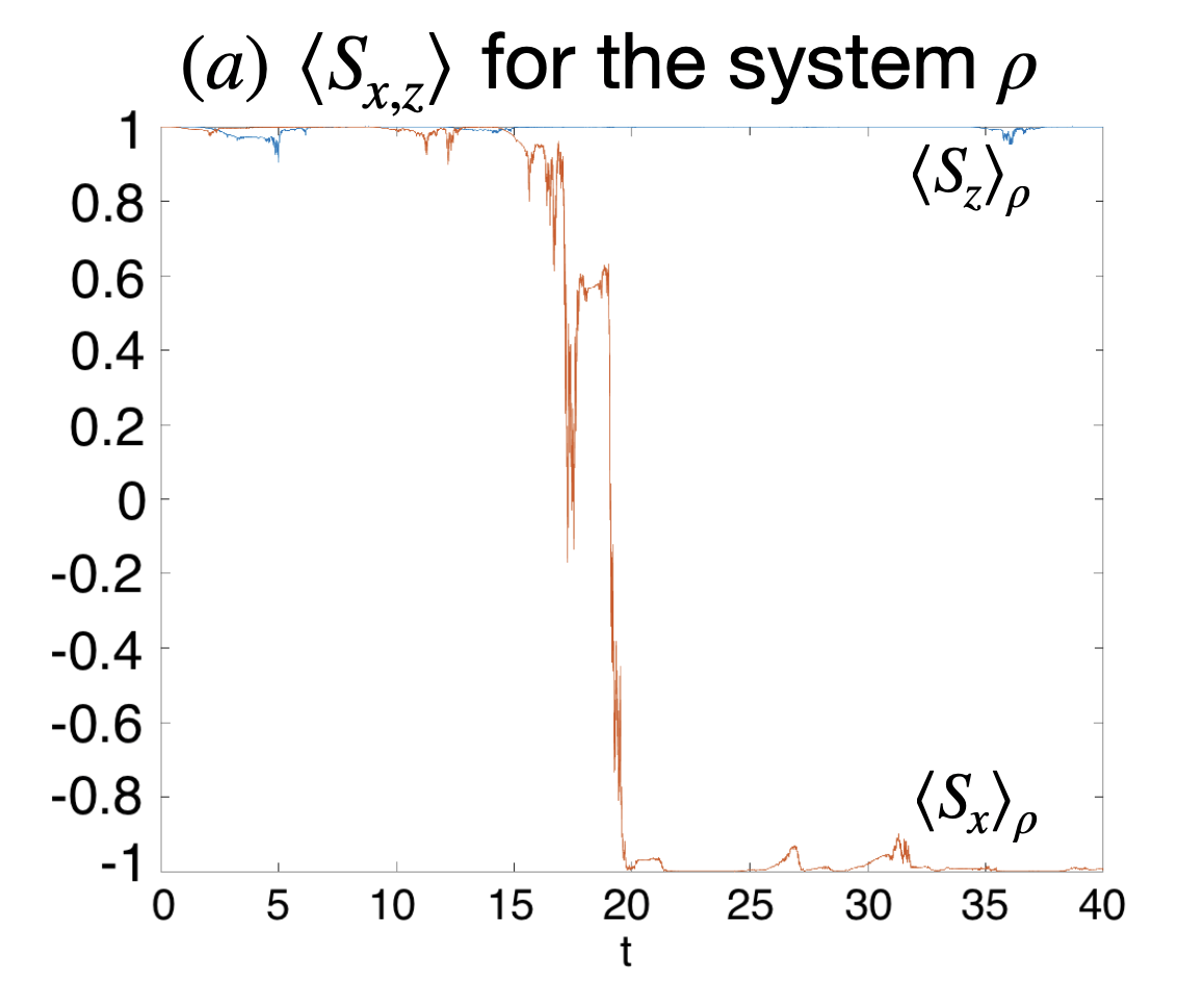
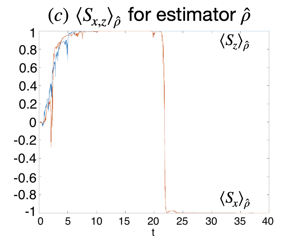
When we apply the four-qubit Bacon-Shor code, we prepare the state in the and eigenspace and store information in the logical qubit of the state. To detect errors, we attach monitor qubits to the system and continuously measure them. If there are no errors, the monitor qubits are static and both converge to 1. Or we can simulate the estimator, which will approach the joint eigenspace. Let us first consider single-qubit errors. Suppose an error happened on the first system qubit. The error anticommutes with and the state is taken to the eigenspace. A sample trajectory is shown in Fig. 4, where the error is detected by observing that drifts to 0 and flips to .
We present another example where the errors are continuous-in-time 1/f Hamiltonian errors, i.e.,
| (34) |
where each is a single-qubit Pauli matrix acting on the th qubit and is a time-dependent scalar function. Each consists of exponentially decaying random pulses with magnitude , i.e.,
| (35) |
where is the Heaviside step function Milotti 2002. In Sec. III.1.2, it is shown that this type of error can be suppressed by implementing continuous indirect measurements. For most trajectories, the system stays close to the eigenspace. converges to while approaches 1 and stays at 1. Occasionally, the error can cause the system to jump to the eigenspace of . A sample trajectory of this case is shown in Fig. 5, where we detect the system’s jumping to by observing that starts to decay to 0 and flips to .

In general, since any single-qubit Pauli error anticommutes with at least one of the , any single-qubit error can be detected. Multi-qubit errors can be detected when they consist of operators anticommuting with one of the . The undetectable errors are those commuting with both . However, they must be at least weight 2. They happen at lower rates than single-qubit errors.
We now consider the cases when errors happen on the monitor qubits. Note that the essential indicator that allows us to distinguish the four eigenspaces of is whether is static or oscillatory in motion. When is , is static. When is , is oscillatory. It turns out that the process of stabilizer detection can be preserved with low rate errors on the monitor qubits. Let us begin with the case of instantaneous errors on the monitor qubits. Suppose an error happened on the monitor . If was static (because the system is in the eigenspace), flips from to but remains static. As shown in Fig. 6, converges to after an error happened at , and then a subsequent error happened at is detected by observing evolving to .

If is oscillatory, an flips the value of but does not change the oscillatory motion. In general, converging to indicates that there was no error, and either converging to indicates there was an error. When such instantaneous errors happen with rates much smaller than , which is approximately the inverse of the measurement time for the indirect detection, the error detection process is preserved. For continuous Hamiltonian errors, since the monitors are being continuously measured, errors with strength much smaller than the measurement rate are partially suppressed by the quantum Zeno effect. Hence, the process of detecting errors on the encoded four-qubit system can be preserved even with low-rate errors on the monitors. However, if the errors happen at high rates, it can cause rapid flipping that mimics the oscillatory effect of , which normally would occur only when . In that limit indirect detection becomes ineffective. Of course, these conclusions are for the particular error model we have been considering. Experimental measurements of the error process might suggest alternative versions of this scheme, e.g., measuring instead of if there are mainly errors.
In the full construction described in Sec. IV, the qubits and are two pairs of physical qubits and . Each pair and is confined to the ground space of the strong base Hamiltonian, . and in the effective Hamiltonian cause transitions only within the ground space, i.e., . Hence they act as for the effective two qubits and . The process of detecting errors for the encoded system is similar: when , both and are static; when , both and are oscillatory. The same applies to and for . We only need to continuously measure one qubit for each pair, e.g., measuring and . If errors can happen on the monitor qubits, it follows similarly from the above argument that the error detection process for the system qubit can be preserved under low-rate errors.
III.1.2 Error suppression


It is well-known that frequent measurements can freeze a system in an eigenspace of the measurement observable due to the quantum Zeno effect. There have been many efforts to harness the Zeno effect for error suppression Paz-Silva et al. 2012; Wüster 2017; Kondo et al. 2016. In Oreshkov and Brun 2007, it is shown that non-Markovian errors can be suppressed by the quantum Zeno effect while Markovian errors can not. In this subsection, we investigate error suppression for various models under continuous indirect measurements. We first consider the 1/f Hamiltonian errors defined in Eq. (34), where the sum is over all physical qubits. In Fig. 7, we plot the ensemble average of the system’s stabilizer values under this 1/f Hamiltonian error. As shown in Fig. 7(a), the red and blue curves represent the case with indirect detection while the purple and yellow curves represent the case without the measurement setup. The pulse rate and are and , where is the strength of the Hamiltonian. The measurement rate is set to . The red and blue curves decay noticeably more slowly than the purple and yellow, which shows that the system state tends to remain in the eigenspace in the presence of indirect stabilizer detection. Note that 1/f Hamiltonian noise is a type of non-Markovian error process. The exhibited suppression aligns with the result in Oreshkov and Brun 2007 that non-Markovian errors can be suppressed by the quantum Zeno effect. We present another example of non-Markovian errors, where the errors are constant Hamiltonian terms, i.e., . To keep the same error magnitude as in the 1/f noise case, the is set to , which is the average strength of in the 1/f noise. The result is shown in Fig. 7(b). Convergence to the joint eigenspace of is apparent when indirect detection is applied.
Another method to benchmark the state protection is to evaluate the trace distance between the state at time and the initial state Paz-Silva et al. 2012.


The smaller the trace distance the closer the state remains to its initial state. Fig. 8 shows a clear protection of the state when the system is being measured.
However, when the errors are Markovian (white noise) the measurements do not appear to fix the stabilizer values, as shown in Fig. 7(c). For Markovian noise, the probability of a state transition is of order for a time step. Errors of this type cannot be suppressed by frequent measurements and full error correction is required to protect the states. For non-Markovian noise, by contrast, the probability of a state transition is of order in a time step. This is why these transitions can be suppressed by the quantum Zeno effect Oreshkov and Brun 2007. The above simulations for continuous indirect measurements agree with these results.
It is worth noting that for the purpose of error prevention, it is possible in principle to suppress Hamiltonian errors by applying a strong Hamiltonian alone. For example, suppose we have a qubit prepared in the state in the basis with the presence of an Hamiltonian error. The error can cause the state to rotate on the y-z plane in the Bloch sphere. However, if we apply a Hamiltonian, which is strong comparing to the error term , the rotating axis becomes closely aligned with the z-axis. The evolution for the state will be confined in a small region near the north pole. The region can be made smaller as we increase the strength for the term. Therefore, the state is maintained close to its initial state . Recall the setup in the indirect measurements. We require interaction Hamiltonians between the system and the monitor qubits. These Hamiltonians also contribute to the suppression of errors because of the above axis-pinning behavior. However, if an error term has a time-dependent coefficient with a frequency component on resonance with energy differences in the system Hamiltonian, transitions are not suppressed. In this case, applying the Hamiltonian alone is not effective against the error. However, applying both the Hamiltonian and the continuous measurements on the monitor qubits performs better in these cases as shown in Fig. 9. Overall, continuous indirect measurements can protect encoded states against errors.

IV Constructing the Hamiltonian for indirect detection
In this section, we show how to build an effective Hamiltonian for indirect detection. The method is based on the idea of perturbation gadgets Jordan and Farhi 2008. It uses 2-local Hamiltonians to produce an effective -local Hamiltonian that appears in the first non-vanishing order for the low-lying energy eigenstates. We begin by briefly recapping the theory presented in Jordan and Farhi 2008.
Suppose we have a strong base Hamiltonian and a weak potential . has zero ground state energy with a degenerate ground space spanned by eigenvectors , and weakly perturbs it. The total Hamiltonian will have a -dimensional vector space spanned by the lowest energy eigenstates . For small enough , largely overlaps with . The space spanned by the lowest energy eigenstates has an effective Hamiltonian
| (36) |
which can be expanded in powers of , i.e.,
| (37) |
The operator projects any vector onto the unperturbed ground space , and the linear operator satisfies
| (38) |
The operator is
| (39) |
where is the projector corresponding to the energy level of the base Hamiltonian . The summation is over nonnegative integers such that and for any from 1 to . and can also be expanded in powers of but only their zeroth order terms, which are both , will contribute in the later discussion. A more detailed derivation of these results can be found in Jordan and Farhi 2008. Note that the expansion converges only if , where is the energy gap between the ground energy (assumed zero) and the second lowest energy. To have a good approximation from the perturbation, we would expect to be much smaller than . In this limit, the effect of adding to becomes a small splitting of the degenerate ground space with a small deviation from the ground space to . When an initial state is prepared in , its evolution stays mainly in and the effective Hamiltonian will be a good approximation for .
The following construction for the indirect measurement requires us to design 2-local Hamiltonian terms and such that the first non-vanishing order of the expansion gives the desired Hamiltonian.
IV.1 First example: detection
Suppose we want to measure for qubits 1 and 2, and the desired Hamiltonian is
We bring in two ancillary qubits and , and turn on a Hamiltonian , where
| (40) |
and the perturbing term is
| (41) |
is a constant and . (Note that the identity term in the base Hamiltonian is unnecessary but we keep it for convenience.) The expansion of in Eq. (37) up to second order in gives
| (42) |
The ancillary qubits are prepared in the ground space, , and the effective Hamiltonian for the 4-qubit system can be approximated by
| (43) |
in the limit of . The shifted term proportional to is neglected since it acts as the identity in the subspace. Note that since the ancillary qubits are restricted to , which is a 2-dimensional subspace, we can treat and as an effective qubit and the operator behaves as that flips . Hence, it can be simplified as a 3-body system with Hamiltonian
| (44) |
which is in the desired form for the indirect measurement (with ). Since and are confined to the ground space and are simultaneously rotated by , we can detect the value of by continuously measure only one of or . When the state is in the eigenspace of , both and are static. When the state is in the eigenspace, and are oscillatory. The system’s value can be obtained by calculating the estimator or evaluating the time average of the signal as described above.
IV.2 Construction for the four-qubit Bacon-Shor code
To indirectly measure the stabilizers, and , for the 4-qubit Bacon-Shor code, we apply the Hamiltonian,
| (45) |
and continuously measure and . However, to obtain this Hamiltonian using only 2-local operators requires four ancillary qubits, which we call and . The full physical system becomes an 8-qubit state, where are the system qubits and are the monitor qubits for the indirect measurements. The full perturbative construction has a Hamiltonian , where the base Hamiltonian is
| (46) |
and the perturbing term is
| (47) |
The monitor qubits are prepared in the ground space of , which consists of two two-level subspaces for the monitors. The unperturbed ground space is . After adding , the perturbed ground space has an effective Hamiltonian that reads
| (48) | ||||
Since the ancillary qubits are prepared in the ground space of , the full system effectively has the Hamiltonian
| (49) |
The and only cause transitions within the ground space , and they act as a single-qubit for an effective qubit confined in the space spanned by . We obtain the target Hamiltonian (45) by identifying and . The monitors are initially prepared in . simultaneously rotates and ( and ) when the state is in the eigenspace. To measure the values of and , we continuously measure (or ) and (or ). The information of the system being in either eigenspace of can be obtained by evaluating and or by calculating using an estimator as described in Sec. II. When the system is in the eigenspace, is static. converges to and . When the system is in the eigenspace, is oscillatory. approaches 0 and . The same detection rule applies to .

It is worth recalling that the constant in the effective Hamiltonian is the strength of the target Hamiltonian in Eq. (45). The fact that needs to be small for the perturbation to work accurately implies that , the strength of the base Hamiltonian, has to be large enough that is large compared to the error strength (or rate). We numerically simulated an example with to demonstrate the performance of the full perturbative construction. The result for is shown in Fig. 10. ( behaves similarly.) The ensemble averages of trajectories for are plotted for various cases. The orange curve represents the no-error case when we apply the full construction using only 2-local Hamiltonians from Eqs. (46) and (IV.2) and continuous measurements of and . When there is no error, is expected to remain 1 throughout the detection process. This is true for the 6-qubit setup introduced in Sec. III. However, building the Hamiltonian perturbatively causes the stabilizers to drop slightly below 1, indicating the presence of small errors due to higher-order corrections. Nonetheless, the deviation is small as shown in Fig. 10. The blue and the green curves are the cases when the system suffers from the 1/f Hamiltonian errors defined in Eq. (34), where the sum is over all physical qubits (including the monitor qubits). The blue includes continuous indirect detection while the green does not. The suppression of errors is apparent, although it is slightly less effective than the ideal 6-qubit case shown in Fig. 7(a). For most trajectories where errors are suppressed, the stabilizer values stay close to 1. For some trajectories where errors cause to flip to , we can detect them by observing decaying towards 0 or flipping to . These behaviors are essentially the same as in Fig. 5.
V Conclusion
We have presented and analyzed a method for the continuous measurement of high-weight operators, and applied this to the problem of continuous quantum error detection by the four-qubit Bacon-Shor code. This method includes engineering an interaction Hamiltonian between the system and the continuously measured ancillary qubits. More nontrivially, the Hamiltonian can be effectively built using physically viable two-local interactions, and the measurements on the monitor qubits consist of well-studied single-qubit continuous measurements.
One major advantage of using this type of continuous monitoring is that it can exhibit error suppression for non-Markovian noise. The traditional circuit-based model is a discrete-time scheme, which cannot generally be carried out quickly enough to produce error suppression. This continuous monitoring scheme does not replace fault-tolerance methods, but it can be incorporated into a larger code (or a larger quantum algorithm) by concatenation. We can implement continuous monitoring for the lowest level qubits and pass the error information to higher levels for error tracing and correction. More specifically, we could encode a qubit at the bottom layer of a large code as the logical qubit of an error-correcting code (or error-detecting code), where the stabilizer generators are continuously monitored by the scheme we introduce here.
In general, this detection scheme can be applied to measuring the stabilizers in any quantum code. However, as the weight of the stabilizers in a code increases, the difficulty of performing this detection scheme is also increased. This is because perturbatively constructing the Hamiltonian for the indirect detection requires applying a strong base Hamiltonian. The strength of this base Hamiltonian grows as the weight of the target term increases because these terms would appear at higher orders in the expansion. This is one of the reasons that we apply it to the four-qubit Bacon-Shor code, where the stabilizers are weight-four and their values can be obtained by measuring the two-local gauge operators. In this case, the target Hamiltonian can appear in the second order expansion, which is the minimum. The question of how the construction scheme applies to other quantum codes remains open, but it should certainly apply to the 9-qubit and larger Bacon-Shor codes.
Two methods are provided for retrieving the measurement outcomes. The estimator approach is computationally hard and difficult to carry out in real time but may be beneficial to theoretical analysis. By contrast, the signal time average is noisier, but more efficient to perform in real time. It is shown that errors with low rates can be detected and (in the non-Markovian case) suppressed. This is in the regime where the indirect detection is effective. For high-rate or high-strength errors that change the system too rapidly, the detection scheme becomes inapplicable. However, if the type of errors can be learned from the experiments, it may be possible to adjust the setup for better performance.
Overall, we have presented a new method for measuring high-weight operators using practical experimental resources. This is a step towards practical quantum error-correction for quantum computing.
Acknowledgements.
TAB and YHC are grateful for useful conversations with Namit Anand, Justin Dressel, Daniel Lidar and Chris Sutherland. YHC acknowledges some of the simulations use the Armadillo C++ library Sanderson and Curtin 2016; Sanderson and Curtin 2018 and are performed on the High-Performance Computing Center at USC. This research was supported in part by NSF Grants QIS-1719778 and FET-1911089.Appendix A Ito rule expansion
Recall from Eqs. (1), (2) and (3) in the paper, we have
| (50) |
where is a constant and will be cancelled out after we normalize the state. We use Ito’s rule, i.e., , and keep terms up to and drop terms of and higher. We then have
| (51) | ||||
and
| (52) |
Combining together these terms, we get
| (53) | ||||
which is Eq. (4) in the paper. Eq. (5) is derived by multiplying both sides of Eq. (4) by the operator and taking the trace. Since , Eq. (5) can be derived as
| (54) |
Appendix B Bayes rule relation
The approximation in Eq. (12) is pure expansion based on the fact that is infinitesimal. To the first order of , the term does not appear. The overall factor is irrelevant to the ratio between in our argument and we do not need to expand it. Let . We have
| (55) |
where is used. Replacing by and going backwards through the above equalities, we get
| (56) |
which shows the Eq. (12).
References
- Wiseman and Milburn (2009) H. M. Wiseman and G. J. Milburn, Quantum Measurement and Control (Cambridge University Press, 2009).
- Jacobs (2014) K. Jacobs, Quantum Measurement Theory and its Applications (Cambridge University Press, 2014).
- Oreshkov and Brun (2005) O. Oreshkov and T. A. Brun, Weak measurements are universal, Phys. Rev. Lett. 95, 110409 (2005).
- Korotkov (1999) A. N. Korotkov, Continuous quantum measurement of a double dot, Phys. Rev. B 60, 5737 (1999).
- Vool et al. (2016) U. Vool, S. Shankar, S. O. Mundhada, N. Ofek, A. Narla, K. Sliwa, E. Zalys-Geller, Y. Liu, L. Frunzio, R. J. Schoelkopf, S. M. Girvin, and M. H. Devoret, Continuous quantum nondemolition measurement of the transverse component of a qubit, Phys. Rev. Lett. 117, 133601 (2016).
- Murch et al. (2013) K. W. Murch, S. J. Weber, C. Macklin, and I. Siddiqi, Observing single quantum trajectories of a superconducting quantum bit, Nature 502, 211 (2013).
- Yang et al. (2020) D. Yang, A. Grankin, L. M. Sieberer, D. V. Vasilyev, and P. Zoller, Quantum non-demolition measurement of a many-body hamiltonian, Nature Communications 11, 775 (2020).
- Korotkov (2001) A. N. Korotkov, Selective quantum evolution of a qubit state due to continuous measurement, Phys. Rev. B 63, 115403 (2001).
- Weber et al. (2014) S. J. Weber, A. Chantasri, J. Dressel, A. N. Jordan, K. W. Murch, and I. Siddiqi, Mapping the optimal route between two quantum states, Nature 511, 570 (2014).
- Atalaya et al. (2017) J. Atalaya, M. Bahrami, L. P. Pryadko, and A. N. Korotkov, Bacon-shor code with continuous measurement of noncommuting operators, Phys. Rev. A 95, 032317 (2017).
- Atalaya et al. (2019) J. Atalaya, A. N. Korotkov, and K. B. Whaley, Error correcting bacon-shor code with continuous measurement of noncommuting operators (2019), arXiv:1910.08272 [quant-ph] .
- Atalaya et al. (2020) J. Atalaya, S. Zhang, M. Y. Niu, A. Babakhani, H. C. H. Chan, J. Epstein, and K. B. Whaley, Continuous quantum error correction for evolution under time-dependent hamiltonians (2020), arXiv:2003.11248 [quant-ph] .
- Paz and Zurek (1998) J. P. Paz and W. H. Zurek, Continuous error correction, Proc. R. Soc. Lond. A. 454, 355 (1998).
- Oreshkov (2013) O. Oreshkov, in Quantum Error Correction, edited by D. A. Lidar and T. A. Brun (Cambridge University Press, 2013) Chap. 8, pp. 201–228.
- Hsu and Brun (2016) K.-C. Hsu and T. A. Brun, Method for quantum-jump continuous-time quantum error correction, Phys. Rev. A 93, 022321 (2016).
- Ahn et al. (2002) C. Ahn, A. C. Doherty, and A. J. Landahl, Continuous quantum error correction via quantum feedback control, Phys. Rev. A 65, 042301 (2002).
- Ahn et al. (2003) C. Ahn, H. M. Wiseman, and G. J. Milburn, Quantum error correction for continuously detected errors, Phys. Rev. A 67, 052310 (2003).
- Ahn et al. (2004) C. Ahn, H. Wiseman, and K. Jacobs, Quantum error correction for continuously detected errors with any number of error channels per qubit, Phys. Rev. A 70, 024302 (2004).
- van Handel and Mabuchi (2005) R. van Handel and H. Mabuchi, Optimal error tracking via quantum coding and continuous syndrome measurement (2005), arXiv:quant-ph/0511221 [quant-ph] .
- Chase et al. (2008) B. A. Chase, A. J. Landahl, and J. Geremia, Efficient feedback controllers for continuous-time quantum error correction, Phys. Rev. A 77, 032304 (2008).
- Gottesman (1997) D. Gottesman, Stabilizer codes and quantum error correction (1997), arXiv:quant-ph/9705052 [quant-ph] .
- Bravyi and Kitaev (1998) S. B. Bravyi and A. Y. Kitaev, Quantum codes on a lattice with boundary (1998), arXiv:quant-ph/9811052 [quant-ph] .
- Fowler et al. (2012) A. G. Fowler, M. Mariantoni, J. M. Martinis, and A. N. Cleland, Surface codes: Towards practical large-scale quantum computation, Phys. Rev. A 86, 032324 (2012).
- Bacon (2006) D. Bacon, Operator quantum error-correcting subsystems for self-correcting quantum memories, Phys. Rev. A 73, 012340 (2006).
- Oreshkov and Brun (2007) O. Oreshkov and T. A. Brun, Continuous quantum error correction for non-markovian decoherence, Phys. Rev. A 76, 022318 (2007).
- Itô (1944) K. Itô, Stochastic integral, Proc. Imp. Acad. 20, 519 (1944).
- Jacobs (2010) K. Jacobs, Stochastic Processes For Physicists (Cambridge University Press, 2010).
- Milotti (2002) E. Milotti, 1/f noise: a pedagogical review (2002), arXiv:physics/0204033 [physics.class-ph] .
- Paz-Silva et al. (2012) G. A. Paz-Silva, A. T. Rezakhani, J. M. Dominy, and D. A. Lidar, Zeno effect for quantum computation and control, Phys. Rev. Lett. 108, 080501 (2012).
- Wüster (2017) S. Wüster, Quantum zeno suppression of intramolecular forces, Phys. Rev. Lett. 119, 013001 (2017).
- Kondo et al. (2016) Y. Kondo, Y. Matsuzaki, K. Matsushima, and J. G. Filgueiras, Using the quantum zeno effect for suppression of decoherence, New Journal of Physics 18, 013033 (2016).
- Jordan and Farhi (2008) S. P. Jordan and E. Farhi, Perturbative gadgets at arbitrary orders, Phys. Rev. A 77, 062329 (2008).
- Sanderson and Curtin (2016) C. Sanderson and R. Curtin, Armadillo: a template-based c++ library for linear algebra, Journal of Open Source Software 1, 26 (2016).
- Sanderson and Curtin (2018) C. Sanderson and R. Curtin, A user-friendly hybrid sparse matrix class in c++, Lecture Notes in Computer Science (LNCS) 10931, 422 (2018).