Residual-driven Fuzzy C-Means Clustering for Image Segmentation
Abstract
Due to its inferior characteristics, an observed (noisy) image’s direct use gives rise to poor segmentation results. Intuitively, using its noise-free image can favorably impact image segmentation. Hence, the accurate estimation of the residual between observed and noise-free images is an important task. To do so, we elaborate on residual-driven Fuzzy C-Means (FCM) for image segmentation, which is the first approach that realizes accurate residual estimation and leads noise-free image to participate in clustering. We propose a residual-driven FCM framework by integrating into FCM a residual-related fidelity term derived from the distribution of different types of noise. Built on this framework, we present a weighted -norm fidelity term by weighting mixed noise distribution, thus resulting in a universal residual-driven FCM algorithm in presence of mixed or unknown noise. Besides, with the constraint of spatial information, the residual estimation becomes more reliable than that only considering an observed image itself. Supporting experiments on synthetic, medical, and real-world images are conducted. The results demonstrate the superior effectiveness and efficiency of the proposed algorithm over existing FCM-related algorithms.
Index Terms:
Fuzzy C-Means, mixed or unknown noise, residual-driven, weighted fidelity, image segmentation.I Introduction
AS an important approach to data analysis and processing, fuzzy clustering has been widely applied to a number of visible domains such as pattern recognition [1, 2], data mining [3], granular computing [4], and image processing [5]. One of the most popular fuzzy clustering methods is a Fuzzy C-Means (FCM) algorithm [6, 7, 8]. It plays a significant role in image segmentation; yet it only works well for noise-free images. In real-world applications, images are often contaminated by different types of noise, especially mixed or unknown noise, produced in the process of image acquisition and transmission. Therefore, to make FCM robust to noise, FCM is refined resulting in many modified versions in two main means, i.e., introducing spatial information into its objective function [9, 10, 11, 12, 13, 14] and substituting its Euclidean distance with a kernel distance (function) [15, 16, 17, 18, 19, 20, 21, 22]. Even though such versions improve its robustness to some extent, they often fail to account for high computing overhead of clustering. To balance the effectiveness and efficiency of clustering, researchers have recently attempted to develop FCM with the aid of mathematical technologies such as Kullback-Leibler divergence [23, 24], sparse regularization [25, 26], morphological reconstruction [24, 27, 28, 29] and gray level histograms [30, 31], as well as pre-processing and post-processing steps like image pixel filtering [32], membership filtering [30] and label filtering [26, 32, 33]. To sum up, the existing studies make evident efforts to improve its robustness mainly by means of noise removal in each iteration or before and after clustering. However, they fail to take accurate noise estimation into account and apply it to improve FCM.
Generally speaking, noise can be modeled as the residual between an observed image and its ideal value (noise-free image). Clearly, its accurate estimation is beneficial for image segmentation as noise-free image instead of observed one can then be used in clustering. Most of FCM-related algorithms suppress the impact of such residual on FCM by virtue of spatial information. So far, there are no studies focusing on developing FCM variants based on an in-depth analysis and accurate estimation of the residual. To the best of our knowledge, there is only one attempt [34] to improve FCM by revealing the sparsity of the residual. To be specific, since a large proportion of image pixels have small or zero noise/outliers, -norm regularization can be used to characterize the sparsity of the residual, thus forming deviation-sparse FCM (DSFCM). When spatial information is used, it upgrades to its augmented version, named as DSFCM_N. Their residual estimation is realized by using a soft thresholding operation. In essence, such estimation is equivalent to noise removal. Therefore, neither of them can achieve highly accurate residual estimation.
To address this issue, we elaborate on residual-driven FCM (RFCM) for image segmentation, which furthers FCM’s performance. We first design an RFCM framework, as shown in Fig. 1(b), by introducing a fidelity term on residual as a part of the objective function of FCM. This term makes residual accurately estimated. It is determined by a noise distribution, e.g., an -norm fidelity term corresponds to Gaussian noise and an -norm one suits impulse noise. In real-world applications, since images are often corrupted by mixed or unknown noise, a specific noise distribution is difficult to be obtained. To deal with this issue, by analyzing the distribution of a wide range of mixed noise, especially a mixture of Poisson, Gaussian and impulse noise, we present a weighted -norm fidelity term in which each residual is assigned a weight, thus resulting in an augmented version namely WRFCM for image segmentation with mixed or unknown noise. To obtain better noise suppression, we also consider spatial information of image pixels in WRFCM since it is naturally encountered in image segmentation. In addition, we design a two-step iterative algorithm to minimize the objective function of WRFCM. The first step is to employ the Lagrangian multiplier method to optimize the partition matrix, prototypes and residual when fixing the assigned weights. The second step is to update the weights by using the calculated residual. Finally, based on the optimal partition matrix and prototypes, a segmented image is obtained.

(a)

(b)
This study makes fourfold contributions to advance FCM for image segmentation:
- •
For the first time, we propose an RFCM framework for image segmentation by introducing a fidelity term derived from a noise distribution into FCM. It relies on accurate residual estimation to greatly improve FCM’s performance, which is absent from existing FCM-related algorithms.
- •
Built on an RFCM framework, we present WRFCM by weighting mixed noise distribution and incorporating spatial information. The use of spatial information makes resulting residual estimation more reliable. It is regarded as a universal RFCM algorithm for coping with mixed or unknown noise.
- •
We design a two-step iterative algorithm to realize WRFCM. Since only vector norm is involved, it is fast by virtue of a Lagrangian multiplier method.
- •
WRFCM is validated to produce state-of-the-art performance on synthetic, medical and real-world images from four benchmark databases.
The originality of this work comes with a realization of accurate residual estimation from observed images, which benefits FCM’s performance enhancement. In essence, the proposed algorithm is an unsupervised method. Compared with commonly used supervised methods such as convolutional neural networks (CNNs) [35, 36, 37, 38, 39, 40] and dictionary learning [41, 42], it realizes the residual estimation precisely by virtue of a fidelity term rather than using any image samples to train a residual estimation model. Hence, it needs low computing overhead and can be experimentally executed by using a low-end CPU rather than a high-end GPU, which means that its practicality is high. In addition, being free of the aid of mathematical techniques, it achieves the superior performance over some recently proposed comprehensive FCMs. Therefore, we conclude that WRFCM is a fast and robust FCM algorithm. Finally, in a mathematical sense, its minimization problem involves an vector norm only. Thus it can be easily solved by using a well-known Lagrangian multiplier method.
II Related Work
In 1984, Bezdek et al. [8] first proposed FCM. So far, it has evolved into the most popular fuzzy clustering algorithm. However, it cannot work well for segmenting observed (noisy) images. It has been improved by mostly considering spatial information [9, 10, 11, 12, 13, 14], kernel distances (functions) [15, 16, 17, 18, 19, 20, 21, 22], and various mathematical techniques [23, 24, 25, 26, 27, 28, 29, 30, 31, 32, 33]. In this paper, we mainly focus on the improvement of FCM with regard to its robustness to noise for image segmentation. Therefore, we introduce related work about it in this section.
II-A FCM with Spatial Information
Over the past two decades, using spatial information to improve FCM’s robustness achieved remarkable successes, thus resulting in many improved versions [9, 10, 11, 12, 13, 14]. For instance, Ahmed et al. [9] introduce a neighbor term into the objective function of FCM so as to improve its robustness by leaps and bounds, thus yielding FCM_S where S refers to “spatial information”. To further improve it, Chen and Zhang [10] integrate mean and median filters into a neighbor term, thus resulting in two FCM_S variants labeled as FCM_S1 and FCM_S2. However, their computing overhead is very high. To lower it, Szilagyi et al. [11] propose an enhanced FCM (EnFCM) where a weighted sum image is generated by the observed pixels and their neighborhoods. Based on it, Cai et al. [12] substitute image pixels by gray level histograms, which gives rise to fast generalized FCM (FGFCM). Although it has a high computational efficiency, more parameters are required and tuned. Krinidis et al. [13] come up with a fuzzy local information C-means algorithm (FLICM) for simplifying the parameter setting in FGFCM. Nevertheless, FLICM considers only non-robust Euclidean distance that is not applicable to arbitrary spatial information.
II-B FCM with Kernel Distance
To address the serious shortcoming of FLICM [13], kernel distances (functions) are used to replace Euclidean distance in FCM. They realize the transformation from an original data space to a new one. As a result, a collection of kernel-based FCMs have been put forward [15, 16, 17, 18, 19, 20, 21, 22]. For example, Gong et al. [15] propose an improved version of FLICM, namely KWFLICM, which augments a tradeoff weighted fuzzy factor and a kernel metric into FCM. Even though it is generally robust to extensive noise, it is more time-consuming than most of existing FCMs. Zhao et al. [20] take a neighborhood weighted distance into account, thus presenting a novel algorithm called NWFCM. Although it runs faster than KWFLICM, its segmentation performance is worse. Moreover, it exhibits lower computational efficiency than other FCMs. More recently, Wang et al. [22] consider tight wavelet frames as a kernel function so as to present wavelet frame-based FCM (WFCM), which takes full advantage of the feature extraction capacity of tight wavelet frames. In spite of its rarely low computational cost, its segmentation effects can be further improved by using various mathematical techniques.
II-C Comprehensive FCM
To keep a sound trade-off between performance and speed of clustering, comprehensive FCMs involving various mathematical techniques has been put forward [23, 24, 25, 26, 27, 28, 29, 30, 31, 32, 33]. For instance, Gharieb et al. [23] present an FCM framework based on Kullback-Leibler (KL) divergence. It uses KL divergence to optimize the membership similarity between a pixel and its neighbors. Yet it has slow clustering speed. Gu et al. [25] report a fuzzy double C-Means algorithm (FDCM) through the utility of sparse representation, which addresses two datasets simultaneously, i.e., a basic feature set associated with an observed image and a feature set learned from a spare self-representation model. Overall, FDCM is robust and applicable to a wide range of image segmentation problems. However, its computational efficiency is not satisfactory. Lei et al. [30] present a fast and robust FCM algorithm (FRFCM) by using gray level histograms and morphological gray reconstruction. In spite of its fast clustering, its performance is sometimes unstable since morphological gray reconstruction may cause the loss of useful image features. More recently, Lei et al. [31] propose an automatic fuzzy clustering framework (AFCF) by incorporating threefold techniques, i.e., superpixel algorithms, density peak clustering and prior entropy. It overcomes two difficulties in existing algorithms [22, 25, 30]. One is to select the number of clusters automatically. The other one is to employ superpixel algorithms and the prior entropy to improve image segmentation performance. However, AFCF’s results are unstable.
In this work, the proposed algorithm differs from all algorithms mentioned above in the sense that we take a wide range of mixed noise estimations as the starting point and directly minimize the objective function of WRFCM formulated by using fidelity without dictionary learning and CNNs and archives outstanding performance in image segmentation tasks.
III FCM and Proposed Methodology
III-A Fuzzy C-Means (FCM)
Given a set , where contains channels, i.e., . FCM is applied to cluster by minimizing:
| (1) |
where is a partition matrix under a constraint for , is a prototype set, stands for Euclidean distance, and denotes a fuzzification exponent ().
Here, is an iterative step and . By presetting a threshold , the procedure stops when .
III-B Noise Model
Consider an observed image with pixels. It is denoted as , where . When , represents a gray image. For , is a Red-Green-Blue color image. Since there is noise in an observed image, can be modeled as a sum of a noise-free image and noise :
| (2) |
Mathematically speaking, is an ideal value of and thus is unknown. is viewed as the residual between and . Its accurate estimation can make instead of participate in clustering so as to improve FCM’s robustness. Hence, it is a necessary step to formulate a noise model before constructing an FCM model. In image processing, the models of single noise such as Gaussian, Poisson and impulse noise are widely used. In this work, in order to construct robust FCM, we mostly consider mixed or unknown noise since it is often encountered in real-world applications. Its specific model is unfortunately hard to be formulated. Therefore, a common solution is to assume the type of mixed noise in advance. In universal image processing, two kinds of mixed noise are the most common, refer to mixed Poisson-Gaussian noise and mixed Gaussian and impulse noise. Beyond them, we focus on a mixture of a wide range of noise, i.e., a mixture of Poisson, Gaussian, and impulse noise. We investigate an FCM-related model based on the analysis of the mixed noise model and extend it to image segmentation with mixed or unknown noise.
Formally speaking, a noise-free image is defined in a domain . It is first corrupted by Poisson noise, thus resulting in that obeys a Poisson distribution, or, . Then additive zero-mean white Gaussian noise with standard deviation is added. Finally, impulse noise with a given probability is imposed. Hence, for , an arbitrary element in observed image is expressed as:
| (3) |
where the subset of denotes the region including the missing information of and is assumed to be unknown with each element being drawn from the whole region by Bernoulli trial with . In image segmentation, mixed noise model (3) is for the first time presented.
III-C Residual-driven FCM
Since there exists an unknown amount of noise in an observed image, the segmentation accuracy of FCM is greatly impacted without properly handling it. It is natural to understand that taking a noise-free image (the ideal value of an observed image) as data to be clustered can achieve better segmentation effects. In other words, if noise (residual) can be accurately estimated, the segmentation effects of FCM should be greatly improved. To do so, we introduce a fidelity term on residual into the objective function of FCM. Consequently, an RFCM framework is first presented:
| (4) |
where is a parameter set, which controls the impact of fidelity term on FCM. We rewrite as with , which indicates that has channels and each of them contains pixels. In this work, (gray) or (Red-Green-Blue). From a channel perspective, we have:
| (5) |
The fidelity term guarantees that the solution accords with the degradation process of the minimization of (4). It is determined by a specified noise distribution. For example, when considering Gaussian noise estimation, we use an -norm fidelity term:
where stands for an vector norm. In the presence of impulse noise, we choose an -norm fidelity term:
where denotes an vector norm. For Poisson noise, we take the Csiszár’s I-divergence [43] of from as a fidelity term, i.e.,
For common single noise, i.e., Gaussian, Poisson, and impulse noise, the above fidelity terms lead to a maximum a posteriori (MAP) solution to such noise estimations. In real-world applications, images are generally contaminated by mixed or unknown noise rather than a single noise. The fidelity terms for single noise estimation become inapplicable since the distribution of mixed or unknown noise is difficult to be modeled mathematically. Therefore, one of the main purposes of this work is to design a universal fidelity term for mixed or unknown noise estimation.
III-D Analysis of Mixed Noise Distribution
To reveal the essence of mixed noise distributions, we here consider generic and representative mixed noise, i.e., a mixture of Poisson, Gaussian, and impulse noise. Let us take an example to exhibit its distribution. Here, we impose Gaussian noise () and a mixture of Poisson, Gaussian () and random-valued impulse noise () on image ‘Lena’ with size , respectively. We show original and two observed images in Fig. 2.


(a)

(b)

(c)
As Fig. 2(b) shows, Gaussian noise is overall organized. As a common sense, Poisson distribution is a Gaussian-like one under the condition of enough samples. Therefore, due to impulse noise, mixed noise is disorganized as shown in Fig. 2(c). In Fig. 3, we portray the distributions of Gaussian and mixed noise, respectively.

Fig. 3(a) shows noise distribution in a linear domain. To illustrate a heavy tail intuitively, we present it in a logarithmic domain as shown in Fig. 3(b). Clearly, Poisson noise leads to a Gaussian-like distribution. Nevertheless, impulse noise gives rise to a more irregular distribution with a heavy tail. Therefore, neither norm nor norm can precisely characterize the residual in the sense of the MAP estimation.
III-E Residual-driven FCM with Weighted -norm Fidelity
Intuitively, if the fidelity term can be modified so as to make mixed noise distribution more Gaussian-like, we can still use norm to characterize residual . It means that mixed noise can be more accurately estimated. Therefore, we adopt robust estimation techniques [44, 45] to weaken the heavy tail, which makes mixed noise distribution more regular. In the sequel, we assign a proper weight to each residual , which forms a weighted residual that almost obeys a Gaussian distribution. Given Fig. 4, we use an example for showing the effect of weighting.

Fig. 4(a) shows the distribution of and the fitting Gaussian function based on the variance of . Fig. 4(b) gives the distribution of and the fitting Gaussian function based on the variance of . Clearly, the distribution of in Fig. 4(b) is more Gaussian-like than that in Fig. 4(a), which means that -norm fidelity can work on weighted residual for a MAP-like solution of .
By analyzing Fig. 4, for , we propose a weighted -norm fidelity term for mixed or unknown noise estimation:
| (6) |
where performs element-by-element multiplication of and . For , makes up a weight matrix . Each element is assigned to location . Since it is inversely proportional to residual , it can be automatically determined. In this work, we adopt the following expression:
| (7) |
where is a positive parameter, which aims to control the decreasing rate of .
By substituting (6) into (4) combined with (5), we present RFCM with weighted -norm fidelity (WRFCM) for image segmentation:
| (8) |
When coping with image segmentation problems, since each image pixel is closely related to its neighbors, using spatial information has a positive impact on FCM as shown in [9, 34]. If there exists a small distance between a target pixel and its neighbors, they most likely belong to a same cluster. Therefore, we introduce spatial information into (8), thus resulting in our final objective function:
| (9) |
In (9), an image pixel is sometimes loosely represented by its corresponding index even though this is not ambiguous. Thus, is a neighbor pixel of , stands for a local window centralized in , and represents the Euclidean distance between and .
III-F Minimization Algorithm
Minimizing (9) involves four unknowns, i.e., , , and . According to (7), is automatically determined by . Hence, we can design a two-step iterative algorithm to minimize (9), which fixes first to solve , and , then uses to update . The main task in each iteration is to solve the minimization problem in terms of , and when fixing . Assume that is given. We can apply a Lagrangian multiplier method to minimize (9). The Lagrangian function is expressed as:
| (10) |
where is a set of Lagrangian multipliers. The two-step iterative algorithm for minimizing (9) is realized in Algorithm 1.
| (11) |
The minimization problem (11) can be divided into the following three subproblems:
| (12) |
Each subproblem in (12) has a closed-form solution. We use an alternative optimization scheme similar to the one used in FCM to optimize and . The following result is needed to obtain the iterative updates of and .
Theorem III.1.
Consider the first two subproblems of (12). By applying the Lagrangian multiplier method to solve them, the iterative solutions are presented as:
| (13) |
| (14) |
Proof.
See Appendix. ∎
In the last subproblem of (12), both and appear simultaneously. Since is dependent to , it should not be considered as a constant vector. In other words, is one of neighbors of while is one of neighbors of symmetrically. Thus, is equivalent to . Thus we have:
| (15) |
where represents a function in terms of or . By (15), we rewrite (9) as
| (16) |
According to the two-step iterative algorithm, we assume that in (16) is fixed in advance. When and are updated, the last subproblem of (12) is separable and can be decomposed into subproblems:
| (17) |
By zeroing the gradient of the energy function in (17) in terms of , the iterative solution to (17) is expressed as:
| (18) |
To show the impact of weighted -norm fidelity on FCM, we show an example, as shown in Fig. 5. We impose a mixture of Poisson, Gaussian, and impulse noise ( ) on a noise-free image in Fig. 5(a). We set to 4. The settings of and are discussed in the later section.

(a)

(b)

(c)

(d)

(e)

(f)

(g)

(h)
As shown in Fig. 5, the noise estimation of DSFCM_N in Fig. 5(g) is far from the true one in Fig. 5(f). However, WRFCM achieves a better noise estimation result as shown in Fig. 5(h). In addition, it has better performance for noise-suppression and feature-preserving than DSFCM_N, which can be visually observed from Fig. 5(c) and (d).
Algorithm 1 is terminated when . Based on optimal and , a segmented image is obtained. WRFCM for minimizing (9) is realized in Algorithm 2.
III-G Convergence Analysis
In WRFCM, we set as the termination condition. In order to analyze the convergence of WRFCM, we take Fig. 5 as a case study. We set . In Fig. 6, we draw the curves of and versus iteration step , respectively.

As Fig. 6 indicates, since the prototypes are randomly initialized, the convergence of WRFCM oscillates slightly at the beginning. Nevertheless, it reaches stability after a few iterations. In addition, even though exhibits an oscillating process, keeps decreasing until the iteration stops. To sum up, WRFCM has outstanding convergence since the weight -norm fidelity makes mixed noise distribution estimated accurately so that the residual is gradually separated from observed data as iterations proceed.
IV Experimental Studies
In this section, to show the performance, efficiency and robustness of WRFCM, we provide numerical experiments on synthesis, medical, and other real-world images. To highlight the superiority and improvement of WRFCM over conventional FCM, we also compare it with seven FCM variants, i.e., FCM_S1 [10], FCM_S2 [10], FLICM [13], KWFLICM [15], FRFCM [30], WFCM [22], and DSFCM_N [34]. They are the most representative ones in the field.
IV-A Evaluation Indicators
To quantitatively evaluate the performance of WRFCM, we adopt three objective evaluation indicators, i.e., segmentation accuracy (SA) [46], Matthews correlation coefficient (MCC) [47], and Sorensen-Dice similarity (SDS) [48, 49]. Note that a single one cannot fully reflect true segmentation results. SA is defined as:
where and are the -th cluster in a segmented image and its ground truth, respectively. denotes the cardinality of a set. MCC is computed as:
where , , , and are the number of true positive, false positive, true negative, and false negative, respectively. SDS is formulated as:
IV-B Dataset Descriptions
Tested images except for synthetic ones come from four publicly available databases including a medical one and three real-world ones. The details are outlined as follows:
- 1)
BrianWeb11 1 http://www.bic.mni.mcgill.ca/brainweb/: This is an online interface to a 3D MRI simulated brain database. The parameter settings are fixed to 3 modalities, 5 slice thicknesses, 6 levels of noise, and 3 levels of intensity non-uniformity. BrianWeb provides golden standard segmentation.
- 2)
Berkeley Segmentation Data Set (BSDS)22 2 https://www2.eecs.berkeley.edu/Research/Projects/CS/vision/grouping/resources.html [50]: This database contains 200 training, 100 validation and 200 testing images. Golden standard segmentation is annotated by different subjects for each image of size or .
- 3)
Microsoft Research Cambridge Object Recognition Image Database (MSRC)33 3 http://research.microsoft.com/vision/cambridge/recognition/: This database contains 591 images and 23 object classes. Golden standard segmentation is provided.
- 4)
NASA Earth Observation Database (NEO)44 4 http://neo.sci.gsfc.nasa.gov/: This database continually provides information collected by NASA satellites about Earth’s ocean, atmosphere, and land surfaces. Due to bit errors appearing in satellite measurements, sampled images of size contain unknown noise. Therefore, their ground truth is unknown.
IV-C Parameter Settings
Prior to numerical simulations, we report the parameter settings of WRFCM and seven comparative algorithms. Since spatial information is used in all algorithm, a local window of size is selected for all. We set and across all algorithms. The setting of is presented in each experiment.
Except , and , FLICM and KWFLICM are free of any other parameters. However, the remaining algorithms involve different parameters. In FCM_S1 and FCM_S2, is set to 3.8, which controls the impact of spatial information on FCM by following [10]. In FRFCM, an observed image is taken as a mask image. A marker image is produced by a structuring element. WFCM requires one parameter only, which constrains the neighbor term. For DSFCM_N, is set based on the standard deviation of each channel of image data.
As to WRFCM, it requires two parameters, i.e., in (7) and in (9). By analyzing mixed noise distributions, is experimentally set to 0.0008. Since the standard deviation of image data is related to noise levels to some extent [34], we can set in virtue of the standard deviation of each channel. Based on massive experiments, is recommended to be chosen as follows:
where is the standard deviation of the -th channel of . In fact, is equivalently replaced by . Here, we give an example to show the setting of , refer to Fig. 7. We impose a mixture of Poisson, Gaussian, and impulse noise on the first three synthetic images in the second row of Fig. 8 respectively. The noise level is and .
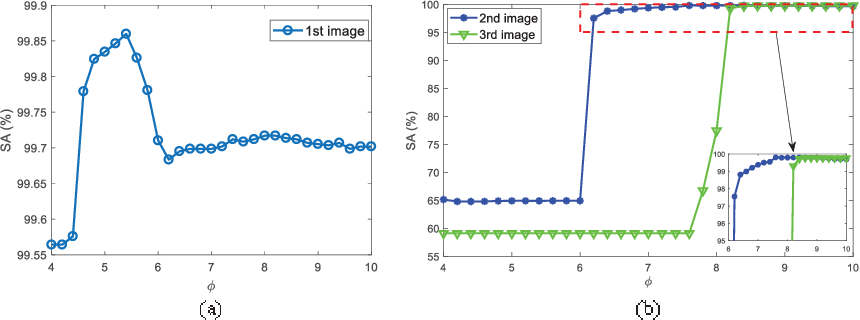
As Fig. 7(a) indicates, when coping with the first image, the SA value reaches its maximum gradually as the value of increases. Afterwards, it decreases rapidly and tends to be stable. As shown in Fig. 7(b), for the other two images, after the SA value reaches its maximum, it has no apparent changes, implying that the segmentation performance is rather stable. In conclusion, for image segmentation, WRFCM can produce better and better performance as parameter increases from a small value.
IV-D Experimental Results and Analysis
IV-D1 Results on Synthetic Images
In the first experiment, we representatively choose five synthetic images of size , as shown in the second row of Fig. 8. A mixture of Poisson, Gaussian, and impulse noise is considered for all cases. To be specific, Poisson noise is first added. Then we add Gaussian noise with . Finally, the random-valued impulse noise with is added since it is more difficult to detect than salt and pepper impulse noise. For five images, we set to 4, 4, 4, 3, and 3, respectively. The segmentation results are given in Fig. 8 and Table I. The best values are in bold.


As Fig. 8 indicates, FCM_S1, FCM_S2 and FLICM achieve poor results in presence of such a high level of mixed noise. Compared with them, KWFLICM, FRFCM and WFCM suppress the vast majority of mixed noise. Yet they cannot completely remove it. DSFCM_N visually outperforms other peers mentioned above. However, it generates several topology changes such as merging and splitting. By taking the second synthetic image as a case, we find that DSFCM_N produces some unclear contours and shadows. Superior to seven peers, WRFCM not only removes all the noise but also preserves more image features.
| Algorithm | Fig. 8 column 1 | Fig. 8 column 2 | Fig. 8 column 3 | Fig. 8 column 4 | Fig. 8 column 5 | ||||||||||
| SA | SDS | MCC | SA | SDS | MCC | SA | SDS | MCC | SA | SDS | MCC | SA | SDS | MCC | |
| FCM_S1 | 92.902 | 98.187 | 96.362 | 92.625 | 98.414 | 95.528 | 87.289 | 99.582 | 97.606 | 94.453 | 97.405 | 95.254 | 90.178 | 97.128 | 95.740 |
| FCM_S2 | 96.157 | 98.999 | 97.991 | 96.292 | 99.127 | 97.520 | 92.345 | 99.791 | 98.808 | 97.214 | 84.356 | 70.353 | 92.737 | 98.518 | 97.769 |
| FLICM | 85.081 | 90.145 | 95.082 | 85.667 | 95.894 | 88.576 | 81.502 | 83.077 | 54.764 | 88.031 | 92.855 | 87.353 | 82.401 | 91.770 | 88.350 |
| KWFLICM | 99.706 | 99.858 | 99.715 | 99.730 | 99.904 | 99.725 | 99.310 | 99.938 | 99.648 | 99.878 | 99.880 | 99.776 | 99.240 | 99.852 | 99.774 |
| FRFCM | 99.652 | 99.920 | 99.839 | 99.675 | 99.895 | 99.698 | 99.629 | 99.924 | 99.568 | 99.751 | 85.222 | 72.048 | 98.883 | 99.726 | 99.581 |
| WFCM | 97.827 | 99.325 | 98.652 | 98.079 | 99.363 | 98.197 | 96.645 | 99.735 | 98.485 | 98.570 | 99.106 | 98.353 | 97.434 | 98.515 | 97.766 |
| DSFCM_N | 98.954 | 99.545 | 99.086 | 99.226 | 99.757 | 99.303 | 98.503 | 99.756 | 98.608 | 99.205 | 85.053 | 71.730 | 99.655 | 99.863 | 99.791 |
| WRFCM | 99.859 | 99.937 | 99.843 | 99.802 | 99.958 | 99.792 | 99.785 | 99.931 | 99.565 | 99.934 | 99.893 | 99.814 | 99.677 | 99.907 | 99.858 |
Table I shows the segmentation results of all algorithms quantitatively. It assembles the values of all three indictors. Clearly, WRFCM achieves better SA results for all images than other peers. In particular, its SA value comes up to 99.934% for the fourth synthetic image. In most cases, it also gets better SDS and MCC results than its seven peers. For the third synthetic image, WRFCM is only slightly inferior to KWFLICM. Among its seven peers, KWFLICM obtains generally better results. In the light of Fig. 8 and Table I, we conclude that WRFCM performs better than its peers.
IV-D2 Results on Medical Images
Next, we representatively segment five medical images from BrianWeb. They are represented as five slices in the axial plane with a sequence of 70, 80, 90, 100 and 110, which are generated by T1 modality with slice thickness of 1mm resolution, 9% noise and 20% intensity non-uniformity. Here, we set for all cases. The comparison between WRFCM and its peers are shown in Fig. 9 and Table II. The best values are in bold.


| Algorithm | Fig. 9 column 1 | Fig. 9 column 2 | Fig. 9 column 3 | Fig. 9 column 4 | Fig. 9 column 5 | ||||||||||
| SA | SDS | MCC | SA | SDS | MCC | SA | SDS | MCC | SA | SDS | MCC | SA | SDS | MCC | |
| FCM_S1 | 75.756 | 97.852 | 96.225 | 75.026 | 98.109 | 96.656 | 79.792 | 98.452 | 97.334 | 81.887 | 98.614 | 97.680 | 81.869 | 94.254 | 90.947 |
| FCM_S2 | 75.769 | 98.119 | 96.664 | 74.970 | 98.176 | 96.765 | 79.886 | 98.458 | 97.338 | 82.073 | 98.625 | 97.695 | 81.788 | 98.223 | 97.195 |
| FLICM | 74.998 | 98.070 | 96.568 | 74.185 | 98.122 | 96.660 | 79.099 | 98.515 | 97.432 | 81.447 | 98.627 | 97.691 | 81.668 | 98.273 | 97.260 |
| KWFLICM | 74.840 | 98.259 | 96.878 | 73.839 | 97.860 | 96.190 | 79.560 | 98.453 | 97.316 | 81.887 | 98.482 | 97.443 | 81.370 | 98.297 | 97.286 |
| FRFCM | 75.853 | 97.620 | 95.775 | 75.514 | 97.660 | 95.830 | 80.283 | 98.278 | 97.013 | 81.852 | 98.319 | 97.171 | 81.666 | 98.079 | 96.945 |
| WFCM | 75.507 | 97.124 | 94.957 | 74.471 | 97.213 | 95.045 | 79.316 | 97.845 | 96.283 | 81.358 | 97.546 | 95.211 | 81.452 | 95.247 | 92.501 |
| DSFCM_N | 76.400 | 92.325 | 86.262 | 75.288 | 91.574 | 85.095 | 79.861 | 97.678 | 95.996 | 81.831 | 93.304 | 88.829 | 81.750 | 94.302 | 91.024 |
| WRFCM | 82.317 | 98.966 | 98.147 | 82.141 | 98.298 | 96.970 | 83.914 | 98.963 | 98.202 | 83.533 | 99.170 | 98.603 | 84.615 | 98.429 | 97.511 |
By a view of the marked red square in Fig. 9, we find that FCM_S1, FCM_S2, FLICM, KWFLICM and DSFCM_N are vulnerable to noise and intensity non-uniformity. They give rise to the change of topological shapes to some extent. Unlike them, FRFCM and WFCM achieve sufficient noise removal. However, they produce overly smooth contours. Compared with its seven peers, WRFCM can not only suppress noise adequately but also acquire accurate contours. Moreover, it yields the visual result closer to ground truth than its peers. As Table II shows, WRFCM obtains optimal SA, SDS and MCC results for all five medical images. As a conclusion, it outperforms its peers visually and quantitatively.
IV-D3 Results on Real-world Images
In order to demonstrate the practicality of WRFCM for other image segmentation, we typically choose two sets of real-world images in the last experiment. The first set contains five representative images from BSDS and MSRC. There usually exist some outliers, noise or intensity inhomogeneity in each image. For all tested images, we set . The segmentation results of all algorithms are shown in Fig. 10 and Table III.
| Algorithm | Fig. 10 column 1 | Fig. 10 column 2 | Fig. 10 column 3 | Fig. 10 column 4 | Fig. 10 column 5 | ||||||||||
| SA | SDS | MCC | SA | SDS | MCC | SA | SDS | MCC | SA | SDS | MCC | SA | SDS | MCC | |
| FCM_S1 | 86.384 | 89.687 | 69.705 | 50.997 | 66.045 | 2.724 | 67.289 | 72.570 | 32.232 | 80.688 | 88.159 | 49.369 | 78.717 | 47.696 | 48.874 |
| FCM_S2 | 86.138 | 79.701 | 69.208 | 51.433 | 12.089 | 2.951 | 67.105 | 59.523 | 31.941 | 80.657 | 47.557 | 49.256 | 78.365 | 86.449 | 47.881 |
| FLICM | 86.476 | 89.771 | 69.882 | 55.292 | 70.055 | 2.403 | 89.233 | 91.167 | 78.117 | 80.771 | 47.826 | 49.729 | 80.617 | 54.490 | 54.029 |
| KWFLICM | 87.119 | 90.278 | 71.283 | 48.252 | 63.432 | 1.554 | 64.617 | 66.081 | 30.820 | 80.484 | 46.723 | 48.777 | 77.963 | 44.791 | 46.755 |
| FRFCM | 97.701 | 98.235 | 94.941 | 99.690 | 97.436 | 97.273 | 99.380 | 99.467 | 98.732 | 83.974 | 89.927 | 58.683 | 96.985 | 97.861 | 92.987 |
| WFCM | 98.442 | 97.755 | 96.563 | 99.688 | 99.834 | 97.268 | 99.295 | 99.160 | 98.555 | 84.480 | 62.664 | 60.043 | 96.445 | 93.943 | 91.719 |
| DSFCM_N | 93.116 | 90.279 | 84.987 | 50.688 | 11.093 | 0.638 | 92.101 | 90.791 | 83.922 | 50.858 | 60.181 | 0.506 | 95.412 | 92.319 | 89.179 |
| WRFCM | 98.732 | 98.162 | 97.201 | 99.746 | 97.906 | 97.771 | 99.442 | 99.520 | 98.857 | 99.826 | 99.888 | 99.074 | 99.869 | 99.789 | 99.694 |


Fig. 10 visually shows the comparison between WRFCM and seven peers while Table III gives the quantitative comparison. Apparently, WRFCM achieves better segmentation results than its peers. FCM_S1, FCM_S2, FLICM, KWFLICM and DSFCM_N obtain unsatisfactory results on all tested images. Superior to them, FRFCM and WFCM preserve more contours and feature details. From a quantitative point of view, WRFCM acquires optimal SA, SDS, and MCC values much more than its peers. Note that it merely gets a slightly smaller SDS value than FRFCM and WFCM for the first and second images, respectively.
The second set contains images from NEO. Here, we select two typical images. Each of them represents an example for a specific scene. We produce the ground truth of each scene by randomly shooting it for 50 times within the time span 2000–2019. The visual results of all algorithms are shown in Figs. 11 and 12. The corresponding SA, SDS, and MCC values are given in Table IV.

(a)

(b)

(c)

(d)

(e)

(f)

(g)

(h)

(i)

(a)

(b)

(c)

(d)

(e)

(f)

(g)

(h)

(i)
| Algorithm | Fig. 11 | Fig. 12 | ||||
| SA | SDS | MCC | SA | SDS | MCC | |
| FCM_S1 | 90.065 | 97.060 | 95.106 | 80.214 | 92.590 | 90.329 |
| FCM_S2 | 93.801 | 97.723 | 95.563 | 81.054 | 92.066 | 90.023 |
| FLICM | 90.234 | 97.056 | 95.781 | 81.582 | 92.352 | 90.236 |
| KWFLICM | 85.902 | 80.109 | 76.329 | 95.001 | 96.364 | 95.633 |
| FRFCM | 81.319 | 80.616 | 78.220 | 96.369 | 97.309 | 96.215 |
| WFCM | 95.882 | 98.854 | 97.293 | 97.342 | 97.430 | 97.178 |
| DSFCM_N | 80.131 | 81.618 | 79.597 | 96.639 | 97.936 | 96.436 |
| WRFCM | 99.080 | 99.149 | 98.512 | 98.881 | 98.797 | 97.582 |
Fig. 11 shows the segmentation results on sea ice and snow extent. The colors represent the land and ocean covered by snow and ice per week (here is February 7–14, 2015). We set . Fig. 12 gives the segmentation results on chlorophyll concentration. The colors represent where and how much phytoplankton are growing over a span of days. We choose . As a whole, by seeing Figs. 11 and 12, as well as Table IV, FCM_S1, FCM_S2, FLICM, KWFLICM, and WFCM are sensitive to unknown noise. FRFCM and DSFCM_N produce overly smooth results. Especially, they generate incorrect clusters when segmenting the first image in NEO. Superior to its seven peers, WRFCM cannot only suppress unknown noise well but also retain image contours well. In particular, it makes up the shortcoming that other peers forge several topology changes in the form of black patches when coping with the second image in NEO.
IV-E Performance Improvement
Besides segmentation results reported for all algorithms, we also present the performance improvement of WRFCM over seven comparative algorithms in Table V. Clearly, for all types of images, the average SA, SDS and MCC improvements of WRFCM over other peers are within the value span 0.238%–27.836%, 0.039%–41.989%, and 0.047%–58.681%, respectively.
| Algorithm | Synthetic images | Medical images |
|
| ||||||||||||
| SA | SDS | MCC | SA | SDS | MCC | SA | SDS | MCC | SA | SDS | MCC | |||||
| FCM_S1 | 8.322 | 1.782 | 3.677 | 4.438 | 1.309 | 2.118 | 26.708 | 26.221 | 57.938 | 13.841 | 4.148 | 5.329 | ||||
| FCM_S2 | 4.863 | 3.767 | 7.286 | 4.407 | 0.445 | 0.755 | 26.783 | 41.989 | 58.272 | 11.553 | 4.078 | 5.254 | ||||
| FLICM | 15.275 | 9.177 | 16.950 | 5.024 | 0.444 | 0.764 | 21.045 | 28.390 | 47.687 | 13.072 | 4.268 | 5.038 | ||||
| KWFLICM | 0.238 | 0.038 | 0.047 | 5.004 | 0.494 | 0.864 | 27.835 | 36.791 | 58.681 | 8.528 | 10.736 | 12.066 | ||||
| FRFCM | 0.293 | 2.988 | 5.627 | 4.270 | 0.774 | 1.339 | 3.976 | 2.467 | 9.995 | 10.136 | 10.010 | 10.829 | ||||
| WFCM | 2.100 | 0.716 | 1.484 | 4.883 | 1.769 | 3.087 | 3.852 | 8.381 | 9.689 | 2.368 | 0.830 | 0.811 | ||||
| DSFCM_N | 0.702 | 3.130 | 6.071 | 4.278 | 4.928 | 8.445 | 23.087 | 30.119 | 46.672 | 10.595 | 9.195 | 10.030 | ||||
IV-F Overhead Analysis
In the previous subsections, the segmentation performance of WRFCM is presented. Next, we provide the comparison of computing overheads between WRFCM and seven comparative algorithms in order to show its practicality. For a fair comparison, all experiments are implemented in Matlab on a laptop with Intel(R) Core(TM) i5-8250U CPU of (1.60 GHz) and 8.0 GB RAM. The execution time of all algorithms for segmenting synthetic, medical, real-world images is presented in Table VI. The mean values are in bold. Moreover, we portray them in Fig. 13.
| Image | FCM_S1 | FCM_S2 | FLICM | KWFLICM | FRFCM | WFCM | DSFCM_N | WRFCM |
| Fig. 8 column 1 | 40.453 | 32.367 | 4.131 | 63.069 | 0.255 | 2.387 | 8.245 | 4.313 |
| Fig. 8 column 2 | 44.116 | 38.982 | 4.567 | 72.607 | 0.270 | 5.157 | 7.271 | 4.598 |
| Fig. 8 column 3 | 67.155 | 49.889 | 3.817 | 102.019 | 0.263 | 3.214 | 7.501 | 4.877 |
| Fig. 8 column 4 | 41.030 | 31.835 | 3.560 | 71.339 | 0.236 | 2.536 | 4.561 | 3.873 |
| Fig. 8 column 5 | 37.364 | 32.343 | 3.655 | 120.872 | 0.323 | 2.542 | 4.245 | 3.570 |
| Mean | 46.024 | 37.083 | 3.946 | 85.981 | 0.270 | 3.167 | 6.365 | 4.246 |
| Fig. 9 column 1 | 35.518 | 29.373 | 3.421 | 146.758 | 0.221 | 2.674 | 6.565 | 1.615 |
| Fig. 9 column 2 | 42.423 | 37.351 | 3.508 | 111.133 | 0.272 | 2.695 | 5.007 | 2.024 |
| Fig. 9 column 3 | 23.213 | 26.378 | 3.341 | 109.381 | 0.265 | 2.473 | 4.242 | 1.813 |
| Fig. 9 column 4 | 30.322 | 30.718 | 6.073 | 99.687 | 0.227 | 2.823 | 4.689 | 2.142 |
| Fig. 9 column 5 | 53.060 | 38.189 | 5.382 | 125.533 | 0.223 | 3.884 | 8.439 | 2.565 |
| Mean | 36.907 | 32.402 | 4.345 | 118.498 | 0.242 | 2.910 | 5.789 | 2.032 |
| Fig. 10 column 1 | 46.739 | 52.238 | 4.243 | 229.498 | 1.085 | 5.452 | 10.283 | 9.567 |
| Fig. 10 column 2 | 51.998 | 52.459 | 4.557 | 336.104 | 1.866 | 9.395 | 10.715 | 5.037 |
| Fig. 10 column 3 | 89.086 | 90.724 | 4.049 | 1039.269 | 1.134 | 4.960 | 12.337 | 2.000 |
| Fig. 10 column 4 | 37.832 | 38.430 | 3.203 | 72.786 | 0.892 | 4.011 | 4.986 | 3.943 |
| Fig. 10 column 5 | 29.722 | 27.879 | 4.436 | 180.304 | 0.836 | 3.277 | 6.614 | 3.917 |
| Mean | 51.075 | 52.346 | 4.098 | 371.592 | 1.162 | 5.419 | 8.987 | 4.893 |
| Fig. 11 | 82.535 | 82.880 | 7.509 | 298.926 | 5.815 | 6.644 | 36.648 | 6.977 |
| Fig. 12 | 44.644 | 41.817 | 5.164 | 54.303 | 1.786 | 7.104 | 18.897 | 2.761 |
| Mean | 63.589 | 62.348 | 6.336 | 176.614 | 3.800 | 6.874 | 27.772 | 4.869 |

As Table VI and Fig. 13 show, for gray and color image segmentation, the computational efficiency of KWFLICM is far lower than the others. In contrast, since gray level histograms are considered, FRFCM takes the least execution time among all algorithms. Due to the computation of a neighbor term in each iteration, FCM_S1 and FCM_S2 are more time-consuming than the others except KWFLICM. Even though FLICM, WFCM and DSFCM_N need more computing overheads than FRFCM, they are still very efficient. For color image segmentation, the execution time of DSFCM_N increases dramatically. Compared with most of seven comparative algorithms, WRFCM shows higher computational efficiency. In most cases, it only runs slower than FRFCM. However, the shortcoming can be offset by its better segmentation performance. In a quantitative study, for each image, WRFCM takes 2.642 seconds longer than FRFCM. However, it saves 45.389, 42.035, 0.671, 184.161, 0.583, and 8.218 seconds over FCM_S1, FCM_S2, FLICM, KWFLICM, FRFCM, WFCM, and DSFCM_N, respectively.
V Conclusions and Future Work
For the first time, a residual-driven FCM (RFCM) framework is proposed for image segmentation, which advances FCM research. It realizes favorable noise estimation in virtue of a residual-related fidelity term coming with an analysis of noise distribution. On the basis of the framework, RFCM with weighted -norm fidelity (WRFCM) is presented for coping with image segmentation with mixed or unknown noise. Spatial information is also considered in WRFCM for making residual estimation more reliable. A two-step iterative algorithm is presented to implement WRFCM. Experiments reported for four benchmark databases demonstrate that it outperforms existing FCM variants. Moreover, differing from popular residual-learning methods, it is unsupervised and exhibits a high speed of clustering.
There are some open issues worth pursuing. First, since a tight wavelet frame transform [51, 52, 53] provides redundant representations of images, it can be used to manipulate and analyze image features and noise well. Therefore, it can be taken as a kernel function so as to produce an improved FCM algorithm, i.e., wavelet kernel-based FCM. Second, can the proposed algorithm be applied to a wide range of non-flat domains such as remote sensing [54], ecological systems [55], and transportation networks [56]? How can the number of clusters be selected automatically? Answering them needs more research efforts.
[Proof of Theorem III.1] Consider the first two subproblems of (12). The Lagrangian function (10) is reformulated as
| (19) |
where .
Acknowledgments
This work is supported in part by the Doctoral Students’ Short Term Study Abroad Scholarship Fund of Xidian University, in part by the National Natural Science Foundation of China under Grant Nos. 61873342, 61672400, in part by the Recruitment Program of Global Experts, and in part by the Science and Technology Development Fund, MSAR, under Grant No. 0012/2019/A1.
References
- [1] A. Baraldi and P. Blonda, “A survey of fuzzy clustering algorithms for pattern recognition. I,” IEEE Trans. Syst. Man Cybern. Part B Cybern., vol. 29, no. 6, pp. 778–785, Dec. 1999.
- [2] A. Baraldi and P. Blonda, “A survey of fuzzy clustering algorithms for pattern recognition. II,” IEEE Trans. Syst. Man Cybern. Part B Cybern., vol. 29, no. 6, pp. 786–801, Dec. 1999.
- [3] C. Subbalakshmi, G. Ramakrishna, and S. K. M. Rao, “Evaluation of data mining strategies using fuzzy clustering in dynamic environment,” in Proc. Int. Conf. Adv. Comput., Netw., Informat., 2016, pp. 529–536.
- [4] X. Zhu, W. Pedrycz, and Z. Li, “Granular encoders and decoders: a study in processing information granules,” IEEE Trans. Fuzzy Syst., vol. 25, no. 5, pp. 1115–1126, Oct. 2017.
- [5] M. Yambal and H. Gupta, “Image segmentation using fuzzy c means clustering: A survey,” Int. J. Adv. Res. Comput. Commun. Eng., vol. 2, no. 7, pp. 2927–2929, Jul. 2013.
- [6] J. C. Dunn, “A fuzzy relative of the ISODATA process and its use in detecting compact well-separated clusters,” J. Cybernet., vol. 3, no. 3, pp. 32–57, 1973.
- [7] J. C. Bezdek, Pattern Recognition with Fuzzy Objective Function Algorithms. New York: Plenum Press, 1981.
- [8] J. C. Bezdek, R. Ehrlich, and W. Full, “FCM: The fuzzy C-means clustering algorithm,” Comput. Geosci., vol. 10, no. 2-3, pp. 191–203, 1984.
- [9] M. Ahmed, S. Yamany, N. Mohamed, A. Farag, and T. Moriarty, “A modified fuzzy C-means algorithm for bias field estimation and segmentation of MRI data,” IEEE Trans. Med. Imag., vol. 21, no. 3, pp. 193–199, Aug. 2002.
- [10] S. Chen and D. Zhang, “Robust image segmentation using FCM with spatial constraints based on new kernel-induced distance measure,” IEEE Trans. Syst. Man Cybern. Part B Cybern., vol. 34, no. 4, pp. 1907–1916, Aug. 2004.
- [11] L. Szilagyi, Z. Benyo, S. Szilagyi, and H. Adam, “MR brain image segmentation using an enhanced fuzzy C-means algorithm,” in Proc. 25th Annu. Int. Conf. IEEE EMBS, Sep. 2003, pp. 724–726.
- [12] W. Cai, S. Chen, and D. Zhang, “Fast and robust fuzzy c-means clustering algorithms incorporating local information for image segmentation,” Pattern Recognit., vol. 40, no. 3, pp. 825–838, Mar. 2007.
- [13] S. Krinidis and V. Chatzis, “A robust fuzzy local information C-means clustering algorithm,” IEEE Trans. Image Process., vol. 19, no. 5, pp. 1328–1337, Jan. 2010.
- [14] T. Celik and H. K. Lee, “Comments on “A robust fuzzy local information c-means clustering algorithm”,” IEEE Trans. Image Process., vol. 22, no. 3, pp. 1258–1261, Mar. 2013.
- [15] M. Gong, Y. Liang, J. Shi, W. Ma, and J. Ma, “Fuzzy C-means clustering with local information and kernel metric for image segmentation,” IEEE Trans. Image Process., vol. 22, no. 2, pp. 573–584, Feb. 2013.
- [16] K. P. Lin, “A novel evolutionary kernel intuitionistic fuzzy C-means clustering algorithm,” IEEE Trans. Fuzzy Syst., vol. 22, no. 5, pp. 1074–1087, Aug. 2014.
- [17] A. Elazab, C. Wang, F. Jia, J. Wu, G. Li, and Q. Hu, “Segmentation of brain tissues from magnetic resonance images using adaptively regularized kernel-based fuzzy-means clustering,” Comput. Math. Method. M., vol. 2015, pp. 1–12, Nov. 2015.
- [18] F. Zhao, L. Jiao, and H. Liu, “Kernel generalized fuzzy c-means clustering with spatial information for image segmentation,” Digit. Signal Process., vol. 23, no. 1, pp. 184–199, Jan. 2013.
- [19] F. Guo, X. Wang, and J. Shen, “Adaptive fuzzy c-means algorithm based on local noise detecting for image segmentation,” IET Image Process., vol. 10, no. 4, pp. 272–279, Apr. 2016.
- [20] Z. Zhao, L. Cheng, and G. Cheng, “Neighbourhood weighted fuzzy c-means clustering algorithm for image segmentation,” IET Image Process., vol. 8, no. 3, pp. 150–161, Mar. 2014.
- [21] X. Zhu, W. Pedrycz, and Z. W. Li, “Fuzzy clustering with nonlinearly transformed data,” Appl. Soft Comput., vol. 61, pp. 364–376, Dec. 2017.
- [22] C. Wang, W. Pedrycz, J. Yang, M. Zhou, and Z. Li, “Wavelet frame-based fuzzy C-means clustering for segmenting images on graphs,” IEEE Trans. Cybern., to be published, doi: 10.1109/TCYB.2019.2921779.
- [23] R. R. Gharieb, G. Gendy, A. Abdelfattah, and H. Selim, “Adaptive local data and membership based KL divergence incorporating C-means algorithm for fuzzy image segmentation,” Appl. Soft Comput., vol. 59, pp. 143–152, Oct. 2017.
- [24] C. Wang, W. Pedrycz, Z. Li, and M. Zhou, “Kullback-Leibler divergence-based Fuzzy C-Means clustering incorporating morphological reconstruction and wavelet frames for image segmentation,” arXiv preprint arXiv:2002.09479, 2020.
- [25] J. Gu, L. Jiao, S. Yang, and F. Liu, “Fuzzy double c-means clustering based on sparse self-representation,” IEEE Trans. Fuzzy Syst., vol. 26, no. 2, pp. 612–626, Apr. 2018.
- [26] C. Wang, W. Pedrycz, M. Zhou, and Z. Li, “Sparse regularization-based Fuzzy C-Means clustering incorporating morphological grayscale reconstruction and wavelet frames,” IEEE Trans. Fuzzy Syst., accepted, Mar. 2020.
- [27] L. Vincent, “Morphological grayscale reconstruction in image analysis: applications and efficient algorithms,” IEEE Trans. Image Process., vol. 2, no. 2, pp. 176–201, Apr. 1993.
- [28] L. Najman and M. Schmitt, “Geodesic saliency of watershed contours and hierarchical segmentation,” IEEE Trans. Pattern Anal. Mach. Intell., vol. 18, no. 12, pp. 1163–1173, Dec. 1996.
- [29] J. Chen, C. Su, W. Grimson, J. Liu, and D. Shiue, “Object segmentation of database images by dual multiscale morphological reconstructions and retrieval applications,” IEEE Trans. Image Process., vol. 21, no. 2, pp. 828–843, Feb. 2012.
- [30] T. Lei, X. Jia, Y. Zhang, L. He, H. Meng, and K. N. Asoke, “Significantly fast and robust fuzzy c-means clustering algorithm based on morphological reconstruction and membership filtering,” IEEE Trans. Fuzzy Syst., vol. 26, no. 5, pp. 3027–3041, Oct. 2018.
- [31] T. Lei, P. Liu, X. Jia, X. Zhang, H. Meng, and A. K. Nandi, “Automatic fuzzy clustering framework for image segmentation,” IEEE Trans. Fuzzy Syst., to be published, doi: 10.1109/TFUZZ.2019.2930030.
- [32] C. Wang, W. Pedrycz, Z. Li, M. Zhou, and J. Zhao, “Residual-sparse Fuzzy C-Means clustering incorporating morphological reconstruction and wavelet frames,” arXiv preprint arXiv:2002.08418, 2020.
- [33] X. Bai, Y. Zhang, H, Liu, and Z. Chen, “Similarity measure-based possibilistic FCM with label information for brain MRI segmentation,” IEEE Trans. Cybern., vol. 49, no. 7, pp. 2618–2630, Jul. 2019.
- [34] Y. Zhang, X. Bai, R. Fan, and Z. Wang, “Deviation-sparse fuzzy c-means with neighbor information constraint,” IEEE Trans. Fuzzy Syst., vol. 27, no. 1, pp. 185–199, Jan. 2019.
- [35] A. Fakhry, T. Zeng, and S. Ji, “Residual deconvolutional networks for brain electron microscopy image segmentation,” IEEE Trans. Med. Imaging, vol. 36, no. 2, pp. 447–456, Feb. 2017.
- [36] K. Zhang, W. Zuo, Y. Chen, D. Meng, and L. Zhang, “Beyond a gaussian denoiser: Residual learning of deep CNN for image denoising,” IEEE Trans. Image Process., vol. 26, no. 7, pp. 3142–3155, Jul. 2017.
- [37] F. Kokkinos and S. Lefkimmiatis, “Iterative residual CNNs for burst photography applications,” in Proc. IEEE Conf. Comput. Vis. Pattern Recognit. (CVPR), Jun. 2019, pp. 5929–5938.
- [38] D. Ren, W. Zuo, D. Zhang, L. Zhang, and M. H. Yang, “Simultaneous fidelity and regularization learning for image restoration,” IEEE Trans. Pattern Anal. Mach. Intell., to be published, doi: 10.1109/TPAMI.2019.2926357.
- [39] Y. Zhang, X. Li, M. Lin, B. Chiu, and M. Zhao, “Deep-recursive residual network for image semantic segmentation,” Neural Comput. Applic., to be published, doi: 10.1007/s00521-020-04738-5.
- [40] K. He, X. Zhang, S. Ren, and J. Sun, “Deep residual learning for image recognition,” in Proc. IEEE Conf. Comput. Vis. Pattern Recognit. (CVPR), Jun. 2016, pp. 770–778.
- [41] J. Jiang, L. Zhang, and J. Yang, “Mixed noise removal by weighted encoding with sparse nonlocal regularization,” IEEE Trans. Image Process., vol. 23, no. 6, pp. 2651–2662, Jun. 2014.
- [42] P. Zhou, C. Lu, J. Feng, Z. Lin and S. Yan, “Tensor low-rank representation for data recovery and clustering,” IEEE Trans. Pattern Anal. Mach. Intell., to be published, doi: 10.1109/TPAMI.2019.2954874.
- [43] T. Le, R. Chartrand, and T. J. Asaki, “A variational approach to reconstructing images corrupted by Poisson noise,” J. Math. Imag. Vis., vol. 27, no. 3, pp. 257–263, Apr. 2007.
- [44] P. J. Huber, “Robust regression: Asymptotics, conjectures and Monte Carlo,” Ann. Stat., vol. 1, no. 5, pp. 799–821, 1973.
- [45] P. J. Huber, Robust Statistics. New York: Wiley, 1981.
- [46] C. Li, R. Huang, Z. Ding, J. C. Gatenby, D. N. Metaxas, and J. C. Gore, “A level set method for image segmentation in the presence of intensity inhomogeneities with application to MRI,” IEEE Trans. Image Process., vol. 20, no. 7, pp. 2007–2016, Jul. 2011.
- [47] D. N. H. Thanh, D. Sergey, V. B. S. Prasath, and N. H. Hai. “Blood vessels segmentation method for retinal fundus images based on adaptive principal curvature and image derivative operators,” Int. Arch. Photogramm. Remote Sens. Spatial Inf. Sci., vol. XLII-2/W12, pp. 211–218, May 2019. doi: 10.5194/isprs-archives-XLII-2-W12-211-2019
- [48] D. N. H. Thanh, U. Erkan, V. B. S. Prasath, V. Kumar, and N. N. Hien, “A skin lesion segmentation method for dermoscopic images based on adaptive thresholding with normalization of color models,” in Proc. IEEE 6th Int. Conf. Electr. Electron. Eng., Apr. 2019, pp. 116–120.
- [49] A. A. Taha and A. Hanbury, “Metrics for evaluating 3D medical image segmentation: analysis, selection, and tool,” BMC Med. Imaging, vol. 15, no. 29, pp. 1–29, Aug. 2015.
- [50] P. Arbelaez, M. Maire, C. Fowlkes and J. Malik, “Contour detection and hierarchical image segmentation,” IEEE Trans. Pattern Anal. Mach. Intell., vol. 33, no. 5, pp. 898-916, May 2011.
- [51] C. Wang and J. Yang, “Poisson noise removal of images on graphs using tight wavelet frames,” Visual Comput., vol. 34, no. 10, pp. 1357–1369, Oct. 2018.
- [52] J. Yang and C. Wang, “A wavelet frame approach for removal of mixed Gaussian and impulse noise on surfaces,” Inverse Probl. Imaging, vol. 11, no. 5, pp. 783–798, Oct. 2017.
- [53] C. Wang, Z. Yan, W. Pedrycz, M. Zhou, and Z. Li, “A weighted fidelity and regularization-based method for mixed or unknown noise removal from images on graphs,” IEEE Trans. Image Process., vol. 29, no. 1, pp. 5229–5243, Dec. 2020.
- [54] T. Xu, L. Jiao, and W. J. Emery, “SAR image content retrieval based on fuzzy similarity and relevance feedback,” IEEE J. Sel. Topics Appl. Earth Observ. Remote Sens., vol. 10, no. 5, pp. 1824–1842, May 2017.
- [55] C. Wang, J. Chen, Z. Li, E. Nasr, and A. M. El-Tamimi, “An indicator system for evaluating the development of land-sea coordination systems: A case study of Lianyungang port,” Ecol. Indic., vol. 98, pp. 112–120, Mar. 2019.
- [56] Y. Lv, Y. Chen, X. Zhang, Y. Duan, and N. Li, “Social media based transportation research: the state of the work and the networking,” IEEE/CAA J. Autom. Sinica, vol. 4, no. 1, pp. 19–26, Jan. 2017.
![[Uncaptioned image]](2004.07160v2/author_cong.png) |
Cong Wang received the B.S. degree in automation and the M.S. degree in mathematics from Hohai University, Nanjing, China, in 2014 and 2017, respectively. He is currently pursuing the Ph.D. degree in mechatronic engineering, Xidian University, Xi’an, China. He was a Visiting Ph.D. Student with the Department of Electrical and Computer Engineering, University of Alberta, Edmonton, AB, Canada. He is currently a Research Assistant at the School of Computer Science and Engineering, Nanyang Technological University, Singapore. His current research interests include wavelet analysis and its applications, granular computing, and pattern recognition and image processing. |
![[Uncaptioned image]](2004.07160v2/author_witold.png) |
Witold Pedrycz (M’88-SM’90-F’99) received the MS.c., Ph.D., and D.Sci., degrees from the Silesian University of Technology, Gliwice, Poland. He is a Professor and the Canada Research Chair in Computational Intelligence with the Department of Electrical and Computer Engineering, University of Alberta, Edmonton, AB, Canada. He is also with the Systems Research Institute of the Polish Academy of Sciences, Warsaw, Poland. He is a foreign member of the Polish academy of Sciences. He has authored 15 research monographs covering various aspects of computational intelligence, data mining, and software engineering. His current research interests include computational intelligence, fuzzy modeling, and granular computing, knowledge discovery and data mining, fuzzy control, pattern recognition, knowledge-based neural networks, relational computing, and software engineering. He has published numerous papers in the above areas. Dr. Pedrycz was a recipient of the IEEE Canada Computer Engineering Medal, the Cajastur Prize for Soft Computing from the European Centre for Soft Computing, the Killam Prize, and the Fuzzy Pioneer Award from the IEEE Computational Intelligence Society. He is intensively involved in editorial activities. He is an Editor-in-Chief of Information Sciences, an Editor-in-Chief of WIREs Data Mining and Knowledge Discovery (Wiley) and the International Journal of Granular Computing (Springer). He currently serves as a member of a number of editorial boards of other international journals. He is a fellow of the Royal Society of Canada. |
![[Uncaptioned image]](2004.07160v2/author_zhiwu.png) |
ZhiWu Li (M’06-SM’07-F’16) received the B.S. degree in mechanical engineering, the M.S. degree in automatic control, and the Ph.D. degree in manufacturing engineering from Xidian University, Xi’an, China, in 1989, 1992, and 1995, respectively. He joined Xidian University in 1992. He is also currently with the Institute of Systems Engineering, Macau University of Science and Technology, Macau, China. He was a Visiting Professor with the University of Toronto, Toronto, ON, Canada, the Technion-Israel Institute of Technology, Haifa, Israel, the Martin-Luther University of Halle-Wittenburg, Halle, Germany, Conservatoire National des Arts et Métiers, Paris, France, and Meliksah Universitesi, Kayseri, Turkey. His current research interests include Petri net theory and application, supervisory control of discrete-event systems, workflow modeling and analysis, system reconfiguration, game theory, and data and process mining. Dr. Li was a recipient of an Alexander von Humboldt Research Grant, Alexander von Humboldt Foundation, Germany. He is listed in Marquis Who’s Who in the World, 27th Edition, 2010. He serves as a Frequent Reviewer of 90+ international journals, including Automatica and a number of the IEEE Transactions as well as many international conferences. He is the Founding Chair of Xi’an Chapter of IEEE Systems, Man, and Cybernetics Society. He is a member of Discrete-Event Systems Technical Committee of the IEEE Systems, Man, and Cybernetics Society and IFAC Technical Committee on Discrete-Event and Hybrid Systems, from 2011 to 2014. |
![[Uncaptioned image]](2004.07160v2/author_mengchu.png) |
MengChu Zhou (S’88-M’90-SM’93-F’03) received his B.S. degree in Control Engineering from Nanjing University of Science and Technology, Nanjing, China in 1983, M.S. degree in Automatic Control from Beijing Institute of Technology, Beijing, China in 1986, and Ph. D. degree in Computer and Systems Engineering from Rensselaer Polytechnic Institute, Troy, NY in 1990. He joined New Jersey Institute of Technology (NJIT), Newark, NJ in 1990, and is now a Distinguished Professor of Electrical and Computer Engineering. His research interests are in Petri nets, intelligent automation, Internet of Things, big data, web services, and intelligent transportation. He has over 800 publications including 12 books, 500+ journal papers (400+ in IEEE Transactions), 23 patents and 29 book-chapters. He is the founding Editor of IEEE Press Book Series on Systems Science and Engineering and Editor-in-Chief of IEEE/CAA Journal of Automatica Sinica. He is a recipient of Humboldt Research Award for US Senior Scientists from Alexander von Humboldt Foundation, Franklin V. Taylor Memorial Award and the Norbert Wiener Award from IEEE Systems, Man and Cybernetics Society. He is founding Co-chair of Enterprise Information Systems Technical Committee (TC) and Environmental Sensing, Networking, and Decision-making TC of IEEE SMC Society. He has been among most highly cited scholars for years and ranked top one in the field of engineering worldwide in 2012 by Web of Science/Thomson Reuters and now Clarivate Analytics. He is a life member of Chinese Association for Science and Technology-USA and served as its President in 1999. He is a Fellow of International Federation of Automatic Control (IFAC), American Association for the Advancement of Science (AAAS) and Chinese Association of Automation (CAA). |